automatic emotional state detection and analysis on
TRANSCRIPT

Automatic Emotional State Detection and
Analysis on Embedded Devices
A dissertation presented
By
Saeed Turabzadeh
The Brunel University in partial fulfilment of the
requirements for the degree of Master of Philosophy in the
subject of RES Electronic and Computer Engineering (MPhil)
College of Engineering, Design and Physical Sciences
Brunel University London
August 2015

Abstract
From the last decade, studies on human facial emotion recognition revealed
that computing models based on regression modelling can produce
applicable performance. In this study, an automatic facial expression real-
time system was built and tested. The method is used in this study has been
used widely in different areas such as Local Binary Pattern method, which
has been used in many research projects in machine vision, and the K-
Nearest Neighbour algorithm is method utilized for regression modelling. In
this study, these two techniques has been used and implemented on the
FPGA for the first time, on the side and joined together to great the model in
such way to display a continues and automatic emotional state detection
model on the monitor. To evaluate the effectiveness of the classifier
technique for human emotion recognition from video, the model was
designed and tested on MATLAB environment and then MATLAB
Simulink environment that is capable of recognizing continuous facial
expression in real time with a rate of 1 frame per second and implemented
on a desktop PC. It has been evaluated in a testing dataset and the
experimental results were promising with the accuracy of 51.28%. The
datasets and labels used in this study are made from videos which, recorded
twice from 5 participants while watching a video. In order to implement it in
real-time in faster frame rate, the facial expression recognition system was
built on FPGA. The model was built on Atlys™ Spartan-6 FPGA
Development Board. It can perform continuously emotional state
recognition in real time at a frame rate of 30 with the accuracy of 47.44%. A
graphic user interface was designed to display the participant video in real
time and also two dimensional predict labels of the emotion at the same
time. This is the first time that automatic emotional state detection has been
successfully implemented on FPGA by using LBP and K-NN techniques in
such way to display a continues and automatic emotional state detection
model on the monitor.

Declaration
I hereby declare that no part of this thesis has been previously submitted to
this or any other university as part of the requirement for a higher degree.
The work described herein was conducted solely by the undersigned except
for those colleagues and other workers acknowledged in the text.
I, Saeed Turabzadeh, declare and confirm that this thesis titled, ‘Automatic
Emotional State Detection and Analysis on Embedded Devices’ and the
work presented in it are my own:
This work was done wholly while in candidature for a research
degree at Brunel University.
Where I have consulted the published work of others, this is always
clearly attributed.
I have acknowledged all main sources of help.
Where the thesis is based on work done by myself jointly with
others, I have made clear exactly what was done by others and what
I have contributed myself to it.

Acknowledgments
This work would not have been feasible without the help from certain
people so I would like to express my graduate to:
First of all, my supervisor, Dr Hongying Meng who introduced me to the
exciting world of automatic emotional, image processing and embedded
devices, understanding, patience and guided me through this project
making it a very enjoyable trip.
Many friends, at our department and externally, have given me help,
information and inspiration in several parts of my work and providing a
productive, stimulating and helpful environment, making my work easier in
all aspects.
I am very grateful to my wife, Azadeh who provided a motivating
environment, encouraged and sacrifices my academic studies. My family for
the support they gave me through my studies.

Supporting Publications
Conference Papers
1. (2014) Jan A, Meng H, Gaus YFA, Zhang F, Turabzadeh S,
Automatic Depression Scale Prediction using Facial Expression
Dynamics and Regression, Proceedings of the 4th International
Workshop on Audio/Visual Emotion Challenge (AVEC14). ACM,
ACM New York, NY, USA. 07 Nov 2014, 73-80.
2. (2015) Gaus YFBA., Meng H, Jan A, Zhang F and Turabzadeh S,
Automatic Affective Dimension Recognition from Naturalistic
Facial Expressions Based on Wavelet Filtering and PLS Regression,
IEEE FG2015 Workshop (EmoSPACE 2015), Ljubljana, Slovenia,
4-8th May, 2015. Proceedings of FG2015.

Contents
List of Figures ............................................................................................................. i
List of Tables ............................................................................................................ iii
List of Symbols ......................................................................................................... iv
1. Introduction .......................................................................................................... 1
1.1 Background ..................................................................................................... 1
1.2 Research Aim and Objectives .......................................................................... 5
1.3 Thesis Structure .............................................................................................. 6
2. Literature Review .................................................................................................. 7
2.1 Human Emotion .............................................................................................. 7
2.2 Affective Computing Research ...................................................................... 11
2.3 Theories on Emotions, Affective Dimensions, and Cognition ....................... 16
2.4 Image Processing Methods ........................................................................... 22
2.5 Data Analysis Methodology .......................................................................... 24
2.6 Overview of the Classifier Fusion System ..................................................... 37
2.7 Multiple Classifier Fusion System for Emotion Recognition ......................... 38
3. Facial Expression Recognition System Based on MATLAB .................................. 39
3.1 Visual Representation of Overall Methodology ............................................ 39
3.2 System Inputs and Output ............................................................................ 41
3.3 Data Collection .............................................................................................. 41
3.4 LBP Features Extraction on 10 Videos .......................................................... 43
3.5 Labels of the Two Emotion Dimensions (GTrace) ......................................... 45
3.6 Implementing K-Fold Cross Validation .......................................................... 47
3.7 System Overview and Implementation on MATLAB Simulink ...................... 53
3.8 Summery ....................................................................................................... 56
4. System Implementation on FPGA ....................................................................... 58
4.1 Introduction .................................................................................................. 58
4.2 Top-Level Block Diagram ............................................................................... 60
4.3 Atlys FPGA Board and VmodCAM Camera Sensor ........................................ 61
4.4 RGB to YCrCb (Y or Grayscale) ................................................................... 62

4.5 Implementing LBP on FPGA and Obtaining the Features ............................. 65
4.6 Training Datasets on FPGA ............................................................................ 66
4.7 Implementing K-NN Algorithm on the FPGA ................................................ 68
4.8 Implementing, Compiling and Simulating the Model ................................... 71
4.9 Real-time GUI ................................................................................................ 72
4.10 Speed comparison between the MATLAB Simulink and FPGA
implementation .................................................................................................. 73
4.11 Summery ..................................................................................................... 74
5. Conclusion and Future Work .............................................................................. 76
5.1 Conclusion ..................................................................................................... 76
5.2 Further Work ................................................................................................. 77
References .............................................................................................................. 79
Appendix ................................................................................................................. 89
Appendix A .......................................................................................................... 89
Appendix B .......................................................................................................... 90
i
List of Figures
Figure 2. 1- Connection between Facial Muscles and Emotional States .................. 9
Figure 2. 2- Darwin Detection of the Facial Expressions for Human Infants .......... 10
Figure 2. 3- Sample of Mood and Frame on Facial Expression ............................... 12
Figure 2. 4- Displays the Four Facial Expressions Employed for Exercise Advisor .. 13
Figure 2. 5- Sensors Exposed to be Effective Indicators ......................................... 14
Figure 2. 6- Fong Definition a Development of Social and Collective Robots ......... 15
Figure 2. 7- First Different Social Robots ................................................................ 16
Figure 2. 8- The Group-Oriented U-Bots Robots..................................................... 16
Figure 2. 9- Facial Action Coding System ................................................................ 19
Figure 2. 10- An Example of a Feeltrace Exhibition ................................................ 20
Figure 2. 11- Convert RGB Image to Grayscale Image ............................................ 27
Figure 2. 12- Centre Pixel Arrangement along the Image....................................... 27
Figure 2. 13- Comparison of the Centre Pixel with Its Neighbour .......................... 28
Figure 2. 14- Arrangement and Transform Binary Values into a Vector Array ....... 29
Figure 2. 15- Local Binary Pattern of an Image ....................................................... 29
Figure 2. 16- Border Pixel Arraignments in LBP Image ........................................... 30
Figure 2. 17- All Steps of Obtaining a Histogram of a RGB Image .......................... 30
Figure 2. 18- An Example of Histogram of an Image .............................................. 31
Figure 2. 19- All Type of Correlation Coefficient ..................................................... 34
Figure 2. 20- Discrete Data Arrangement of FeelTrace .......................................... 35
Figure 2. 21- A High-Level Overview of the Classifier Fusion System for Automatic
Human Emotion Recognition .................................................................................. 37
Figure 3. 1- Visual Representation of Overall Methodology .................................. 39
Figure 3. 2- Two Captures of the Video Watched By Participants .......................... 41
Figure 3. 3- Faces of the Participants in the Experiment ........................................ 42
Figure 3. 4- Local Binary Pattern (LPB) MATLAB Code ............................................ 43
Figure 3. 5- An Example of one Frame RGB and LBP View with its Features ......... 44
Figure 3. 6- Feeltrace Exhibition ............................................................................. 45
Figure 3. 7- An Example of Valence Over View in GTrace Environment ................. 46
Figure 3. 8- Activation and Valence of a Video ....................................................... 46
Figure 3. 9- Predict and Actual Labels of 2 Fold Cross Validation ........................... 50
Figure 3. 10- Visual Representation of MATLAB Simulink Model ........................... 54
Figure 3. 11- The Outputs of MATLAB Simulink Model .......................................... 55
Figure 3. 12- Simulink Profile Report for the LBP Block .......................................... 56
Figure 3. 13- Visual Representation of MATLAB Simulink Model Real Time .......... 56
Figure 4. 1- A High-Level of Overall Methodology .................................................. 60
Figure 4. 2 - Visual Representation of Hardware Realization ................................. 61
ii
Figure 4. 3- Ports Layout of the Atlys Spartan-6 FPGA Board ................................. 61
Figure 4. 4- Xilinx LogiCORE IP RGB to YCrCb Colour-Space Converter V3.0 .......... 64
Figure 4. 5- RGB to Grayscale Conversion on FPGA ................................................ 64
Figure 4. 6- Parallel LBP Implementation on FPGA ................................................. 66
Figure 4. 7- All Dataset (Features, Labels) Saved In .Coe File ................................. 67
Figure 4. 8- Xilinx LogiCORE IP Block Memory Generator V6.2 .............................. 67
Figure 4. 9- Xilinx LogiCORE IP Multiplier V11.2 ..................................................... 69
Figure 4. 10- Xilinx LogiCORE IP Cordic V.4 ............................................................. 69
Figure 4. 11- An Example of VHDL Code for Findig the Five Least Distances in the
Row Vector .............................................................................................................. 70
Figure 4. 12- Xilinx LogiCORE IP Division Generator v3.0 ....................................... 70
Figure 4. 13- Predict and Actual Labels of 2 Fold Cross Validation ......................... 72
Figure 4. 14- Parallel LBP and K-NN Implementation on FPGA .............................. 73
Figure 4. 15- Comparing Speed of MATLAB and FPGA ........................................... 74

iii
List of Tables
Table 2. 1- Descriptions of Facial Muscles Involved In the Emotions Darwin
Considered Universal ................................................................................................ 9
Table 2. 2- Confusion Matrix Arrangement ............................................................ 36
Table 3. 1- Details of the Parts in the Video ........................................................... 42
Table 3. 2- Average Correlation Coefficient of 5 Fold Cross Validation .................. 49
Table 3. 3- Average Correlation Coefficient of 2 Fold Cross Validation .................. 50
Table 3. 4- 4 Zones Confusion Matrix of the 5-Fold Cross Validation ..................... 51
Table 3. 5- 4 Zones Confusion Matrix of the 2-Fold Cross Validation ..................... 52
Table 3. 6- Average Accuracy of Confusion Matrix for Different K ......................... 52
Table 4. 1- VmodCAM Output Formats .................................................................. 62
Table 4. 2- Pixels Arrangement In Order To Obtain the LBP ................................... 65
Table 4. 3- Average Correlation Coefficient of Xilinx Simulation ............................ 71
Table 4. 4- 4 Zones Confusion Matrix of the 2-Fold Cross Validation Xilinx
Simulation ............................................................................................................... 71
iv
List of Symbols
ECG Electrocardiogram
EMG Electromyogram
Resp Respiration
SC Skin Conductivity
FRT Facial Recognition Technology
JAFFE Japanese Female Facial Expression
LBP Local Binary Pattern
K-NN K-Nearest Neighbour
EOH Edge Orientation Histogram
LPQ Local Phase Quantization
MIT Massachusetts Institute of Technology
HCI Human Computer Interaction
FACS Facial Action Coding System
AU Action Units
PPMCC Pearson Product Moment Correlation Coefficient
GPU Graphics Processing Unit
FPGA Field Programmable Gate Array
ASIC Application Specific Integrated Circuit
CLB Configurable Logic Block
OTP One Time Programmable
DSP Digital Signal Processor

1
1. Introduction
1.1 Background
The expression of emotions has been researched extensively in psychology
[1]. Emotions are not the same corporeal moods relevant with attitude,
temperament, personality, essence, and stimulant as well as with hormones
such as serotonin, dopamine, and noradrenaline. Sentimentality is often the
showing energy behind motivation, undesirable or desirable. The most
scholars have proposed biologically rational neural architectures for facial
emotion recognition [2].
The emotion recognition was presented, over and done with intended
researches with human observers [3] [4]. Automatic recognition and study
of the facial emotional status expresses significant hints for the manner in
which a person behaves next and is very beneficial for observing, checking
and keeping safe vulnerable people like patients who receiving mental
treatment, someone tolerating substantial mental pressure, and kids without
enough ability to control oneself. With emotion recognition capability,
apparatus such as computers, robots, toys and game consoles will have
ability to act in such a way, to have an effect on the consumer in adaptive
ways depending on consumers’ mental situation. It is the key technology in
recently proposed new concepts such as emotional computer, emotion-
sensing smart phones and emotional robots [5].
Over the last decade, most studies have concentrated on emotional signs in
facial expressions. In recent years, researches have also started to study
effectively conveying thought or feeling of body language. A perception
thought shared to the work on feeling of body language is only a deferent
income of stating the same set of basic emotions as facial expressions. The
identification of entire body languages is significantly more difficult, as the
2
shape of the human body has more points of freedom than the face, and its
general shape differs muscularly through expressed motion.
In the 19th century, one of the significant works on facial expression
analysis that has a straight association to the current day science of
automatic facial expression recognition was the effort done by Charles
Darwin. In 1872, he wrote a dissertation that recognized the general values
of expression and the incomes of expressions in both humans and animals
[6]. He grouped several kinds of terms into similar groups. The
classification is as follows:
low spirits, anxiety, grief, dejection and despair
joy, high spirits, love, tender feelings and devotion
reflection, meditation, ill-temper, sulkiness and determination
hatred and anger
disdain, contempt, disgust, guilt and pride
surprise, astonishment, fear and horror
self-attention, shame, shyness and modest
Also, Darwin classified the facial distortions that happen for each of the
above stated classes of expressions. For example: “the constriction of the
muscles around the eyes when in sorrow”, “the stiff closure of the mouth
when in contemplation”, etc. [6]. The maximum efficacy and additional
considerable landmark in researching of facial expressions and human
emotions is the work done by Paul Ekman and his colleagues since 1970s.
Their work was significance and had a massive effect on the development
on present-day automatic facial expression recognizers.
The early study in the way of the automatic recognition of facial expressions
was occupied in 1978 by Suwa et al. He generated a model for studying on
facial expressions from a sequence of pictures by employing twenty
tracking arguments of points. There were researches until the end of 1980s
and early 1990s, when economy computing power on the go become
3
available. This helped to growth the face detection and face tracking
algorithms in the early 1990s. At the same time, Human Computer
Interaction (HCI) and Affective Computing started.
Emotional state analysis is more likely a phycology field. However, due to
more and more computing methods have been successfully used in this area,
it has been merged into a computing topic with a new name of “affective
computing” [7]. Signal, image processing and pattern recognition methods
deliver a fundamental role for efficient computing. Firstly, emotional state
of a person can be detected from their facial expression, speech and body
gesture by imaging systems. Secondly, the features can be extracted from
these recordings based on signal and image processing methods. Finally,
advanced pattern recognition methods are applied to recognize the
emotional states. Automatic emotional states detection and recognition has
made big progress recently with existed evidence such as emotional
computer proposed by Cambridge University [8] and Mood Meter [9] built
by MIT. In 2011, two international challenges/workshops have been held
and the researchers all over the world competed for the best automatic
emotional state recognition system evaluated on the same recording data
[10] [11].
However, most emotional state recognition systems have suffered from the
lack of real-time computing ability due to algorithm complexities. It
prevents current systems to be used for real-world applications, especially
for low-cost, low-power consumption and portable systems. Nowadays,
multi-core computer, GPU, and embedded devices have got more power and
the ability for computing acceleration. Many computer vision and pattern
recognition algorithms have been implemented on embedded systems in
real-time based on parallelization in algorithms and hardware processing
architectures. Embedded devices provide a new platform for a real-time
automatic emotional state detection and recognition system.
However in 2013 Cheng J, Deng Y, Meng H and Wang Z built a system on
PC based continuous emotional state monitoring system that is able to

4
recognize naturalistic facial expression in a dimensional space was designed
and implemented. A key feature of their proposed system is the capability of
real-time processing by using GPU as an accelerator. It has been tested in
real-world movie watching scenarios and the results prove to be promising
[82]. The proposed system was initially implemented under MATLAB. It
has been found that the processing speed is not sufficient for real-time
processing. Since GPUs have already been widely used as a general purpose
platform to accelerate time-consuming applications, they choose to port the
feature extraction part of the system on GPU. Their system can be speed up
to 80 times faster on GPU compare with CPU speed depends on the
resolution of data. However their system can analyse and produce the
emotional state detection every 1.5 second [82].
Microsoft Project Oxford built an online service to recognize emotions
detect emotions based on facial expressions [83]. The Emotion API takes an
image as an input, and returns the confidence across a set of emotions for
each face in the image, as well as bounding box for the face, using the Face
API. If a user has already called the Face API, they can submit the face
rectangle as an optional input.
Image resolution should be less than 36x36 pixels and the file size
support up to 4MB, Supported image formats include: JPEG, PNG,
GIF (the first frame), BMP.
The frontal and near-frontal faces have the best results. And the
maximum returning faces is set to 64 for each image.
The emotions detected are anger, contempt, disgust, fear, happiness, neutral,
sadness, and surprise. These emotions are understood to be cross-culturally
and universally communicated with particular facial expressions.
Recognition is experimental and not always accurate [83].
This is the first time that automatic emotional state detection has been
successfully implemented on embedded device (FPGA). To compare with
the other system that mention previously, the system has a capability to

5
works on real time video inputs with an ability of analysis 30 frames per-
second compare with the Cheng J, Deng Y, Meng H and Wang Z system the
system on the FPGA is producing predict labels on the output 20 times
faster. The model works with real time video capturing this despite that the
Microsoft API emotions detection’s processing capabilities is only on the
single image at the time, while the system on the embedded device is
continues and automatic emotional state detection model.
The method is used in this study has been used widely in different areas
such as Local Binary Pattern (LBP) method, which has been used in many
research projects in machine vision. LBP algorithm performs well with face
images due to its alteration of the image into an arrangement of micro-
patterns [57]. On the other hand the, in regression technique, the K-Nearest
Neighbour algorithm (K-NN) is method utilized for regression modelling
[81]. This algorithm is a based on learning, where the operation is only
approximated nearby the training dataset and all calculation is delayed until
regression. The K-NN method is the simplest of all machine learning
algorithms [62]. In this study, these two techniques has been used and
implemented on the FPGA for the first time, on the side and joined together
to great the model in such way to display a continues and automatic
emotional state detection model on the monitor.
1.2 Research Aim and Objectives
Aim
The aim of this project is to investigate the issue on how to make the best
use of FPGA for achieving real-time performance in automatic emotional
state detection and recognition systems.
The objectives of this timely proposal are to:
Design a high performance automatic emotional state recognition
system in a simulation environment

6
Investigate the best solutions of suitable software-hardware system
design based on FPGA
Implement an automatic emotional states detection and analysis
demo system on an embedded hardware device
1.3 Thesis Structure
To fulfil the above objectives, the chapters presented in this thesis are as
follows:
Chapter 2 contains an appraisal of the numerous techniques that have been
used in the expansion of face recognition systems. Statistical methods are
discussed. The resulting explanation as to why features extraction and
regression technique used to develop a model for continuously emotional
state recognition in real time presented in this thesis. Introduces the system
overview, and discusses the three main stages of the system – the data
extraction, the classifier function and the output processing. Also materials
and theory used to implement the model are explained and discussed.
Chapter 3 presents how the methods being applied to the system for face
recognition systems. The method of presentation of results in this thesis is
discussed and the values that will be presented in this chapter and in the
later chapters.
Chapter 4 presents the methodology as a face recognition system on FPGA,
and how the training databases id added to the system, how the K-NN
regression implemented on FPGA is presented and discussed in detail.
Chapter 5 concludes the different chapters that have been covered in this
thesis, and delivers a summary of the problems faced for how to get the data
out from FPGA. Future progresses using the methods are also identified.
7
2. Literature Review
2.1 Human Emotion
“There is no Passion, but some particular gesture
of the eyes declare it… though a man may easily
perceive these gestures of the eyes, and know what
they signify, it is not an easy matter to describe them,
because every one of them is composed of several
alterations…so small that each of them cannot be
discerned distinctly, though the results of their conjunction can be easily
marked” [12].
The word "emotion" comes back from a French word “émouvoir”, which it
was adapted in 1579, with meaning of "to stir up". But, the initial
forerunners of the word probable times back to the very roots of language
[13]. Emotions are strong feelings that are absorbed at something or
someone [14].
Although the term “emotion” had not yet been well-defined during the
Enlightenment in the same presentiment as we comprehend nowadays,
concepts of emotions ascended from before modern sources [15]. Efforts to
taxonomize and label emotional states have been used since the time of
Aristotle. In the seventeenth century the words “passion” and “affect”
usually used by philosophers and later the word “sentiment” was used in the
in the eighteenth century to define what contemporary psychologists
understand as affective states. Nowadays, the field of affective science has
developed a monolith field with computer science, of which increased the
amount of work has been done in the field of automatic recognition systems.
The first principle of affective computing is consequently a product of the
impoundment of innovation and scientific knowledge.
In contemporary psychology, affect is known as the experience of sensation
or emotion as different from thought, belief, or action. Therefore, emotion is
8
the sense that a person feels while affect is the state. Scherer defines
emotion as the outcome of reaction synchronization whose output
correspond to an event that is “relevant to the major concerns of the
organism” [16]. Emotion is different from mood in that the earlier has a
strong and clear attention while the latter is unclear, can appear without
reason, and lack severity. Psychologists perceive moods as “diffuse affect
states, characterized by a relative enduring predominance of certain types of
subjective feelings that affect the experience and behaviour of a person”
[16]. Moods may carry for hours or days; due to people character and affect
nature; people practice some moods more often than other people [16].
Consequently it is more problematic to measure situations of mood. On the
other hand, emotion is a quantifiable element due to its separate nature.
Primary attempts to measure and classify feeling through perception of
facial expressions revealed that feelings are not the result of retraction of the
only one muscle, nonetheless particular sets of muscles case facial
expressions revealed that feelings. In 1872 Darwin postulated on his original
work that facial expressions in people were the result of improvement and
that “the study of Expression is difficult, owing to the movements (of facial
muscles) being often extremely slight, and of a fleeting nature” [17].
Notwithstanding this test, early efforts to measure emotions based on facial
expressions in adults and infants. Initial researches on undesirable emotional
states prove that particular features of the eyelids and eyebrows as Darwin
called “the grief-muscles,” agreement in that “oblique position in persons
suffering from deep dejection or anxiety” [18]. However these perceptions
and intentions to classify and categorise facial muscle movement with
separate emotional states, scientists during the 19th century faced with
challenges in recognising distinctions between these features. “A difference
may be clearly perceived, and yet it may be impossible, at least I have found
it so, to state in what the difference consists” [17].
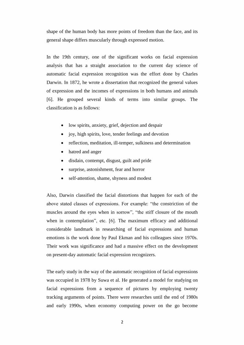
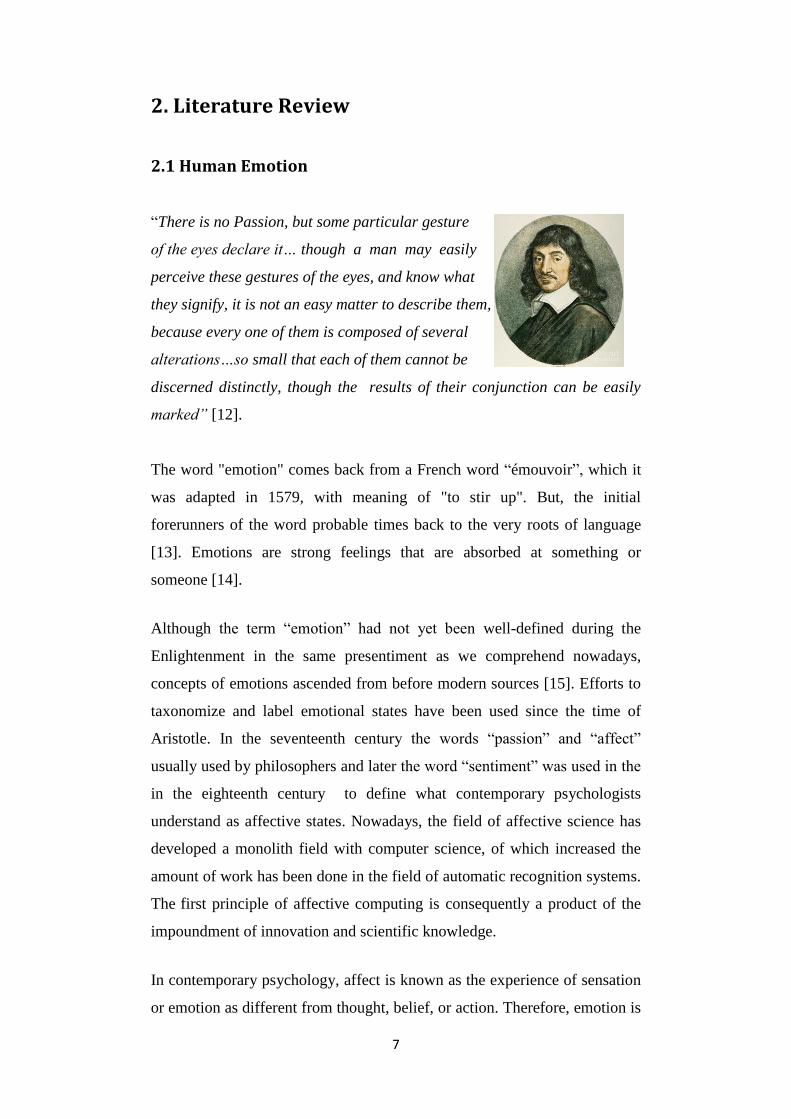
Facial expressions are instrumentation of a consonant repetition involving
many reaction of a model figure 2.1. Darwin considered general facial
muscles, which involved in each of the emotions state, table 2.1.

9
Table 2. 1- Descriptions of Facial Muscles Involved In the Emotions Darwin Considered
Universal [18]
Emotion Darwin’s Facial Description
Fear
eyes open
mouth open
lips retracted
eye brows raised
Anger
eyes wide open
mouth compressed
nostrils raised
Disgust
mouth open
lower lip down
upper lip raised
Contempt
turn away eyes
upper lip raised
lip protrusion,
nose wrinkle
Happiness
eyes sparkle
mouth drawn back at corners
skin under eyes wrinkled
Surprise
eyes open
mouth open
eyebrows raised
lips protruded
Sadness corner mouth depressed
inner corner eyebrows raised
joy
upper lip raised
nose labial fold formed
orbicularis
zygomatic
Figure 2. 1- Connection between Facial Muscles and
Emotional States [18]

10
Charles C. Bell saying that emotion as a principled switch to trigger certain
sets of muscles revealed that feelings on the face; he observed that when
unaffected emotion is expressed, the muscles on the face, which convention
are always the similar muscles and thus the appearance generated is an
outcome of the emotional state. His pluralization his studies that, “opposite
passions” crop dissimilar expressions and consequently positive and
negative emotional states cannot be qualified at the same time1.
Primary studies on facial expressions often focused on human infants. Bell
and Darwin at first have faith in that age effect on adults to lose the aptitude
to express some emotions; therefore they chose to detect the facial
expressions of human infants figure 2.2 [19].
1 “When the angles of the mouth are depressed in grief, the eyebrows are not elevated at the outer
angles, as in laughter. When a smile plays around the mouth, or the cheek is elevated in laughter, the
brows are not raised as in grief. The characters of such opposite passions are so distinct, that they
cannot be combined where there is true and genuine emotion. When we see them united by those who
have a ludicrous control over their muscles, the expression is farcical and ridiculous. It never is by the
affection of an individual feature that emotion is truly expressed” [19]
Figure 2. 2- Darwin Detection of the Facial Expressions for Human Infants [17]
11
2.2 Affective Computing Research
Specified the challenges of identifying emotional states from facial
expressions, 19th century studies on how to recognize human feelings were
typically built on the dissociation between positive and negative
dimensions. The theory supposed that the facial muscles agreement
differently when a person is feeling a positive sentimental state (such as
happiness) versus when someone is experiencing a negative affective state
(such as anger). This interpretation classifies all sentiments as
fundamentally two-dimensional. In the recent thirty years that research in
affect-related arenas (e.g. psychology, psychiatry, cognitive science, and
neuroscience) provided practicalities for researchers and scientists to
thoroughly recognize and identify emotions [20], that emotional computing
has developed an integrative field foreshortening Human-Computer
Interaction layout.
Significant improvements have been completed in the measurement of
individual elements of emotion. Ekman‘s Facial Action Coding System
(FACS) [20] relates observation of particular muscle contractions on the
face with emotions. Scherer et al. measured elements such as assessment
[21], Davidson et al. published comprehensive studies on the relevance
between brain physiology and emotional expressions [22], Stemmler‘s
studies determine and revealed physiological reaction outlines [23],
Harrigan et al. appraisal and measured adequate behaviour [24], and
Fontaine et. al represent that in order to demonstrate the six components of
feelings at least four dimensions are needed [21]. These studies demonstrate
that although emotions are various and multifaceted also often problematic
to classifications, it presents itself via designs that “in principle can be
operationalized and measured empirically” [16]. The hardness of classifying
these patterns is what drives research in emotional computing. In the last
twenty years, a majority of the study in this area has been into enabling
processors and computers to declare and identify affect [25]. Progress made
in emotional computing has not only caused assistances to its own research
field but also benefits in practical domain such as computer interaction.

12
Emotional computing research develops computer interaction by generating
computers to improved serve the desires of users. Meanwhile, it has also
allowed human to perceive computers as something more than merely a data
machine. Upgrading computer interaction over studying in emotional
computing has various benefits. From diminish human users frustration to
assisting machines familiarize to their human users by allowing
communication of user feeling [25], emotional computing enables machines
to become allied operative systems as socially sagacious factors [26].
Figure 2.3 and 2.4, are one of the first examples of a machine operation as a
socially sagacious agent. Figure 2.3 demonstrates several examples of
effects and frame on facial appearance. For example, in the high immediacy,
the representative is showed in a medium shot has a happy facial expression,
and does stare [27] [28].
Figure 2. 3- Sample of Mood and Frame on Facial Expression [27]

13
2.2.1 The State of the Art: Creating Machines with Emotions and
Personalities
To recognize impression in humans, for computers as technologies with no
inherent feelings the sector of computer science and psychology have come
together to create schemes which allow computers to learn, analyse,
identify, and predict human emotions. Study from the state of the art has
exposure devices which effort to sense and detect many data pertaining to
the human face and body. Picard et Al. designed and made skin-superficial
sensors, which collect and measure data related to nervous system
conversions in terms of physiological [27] [28]. Figure 2.5 shows such
sensors have been exposed to be effective indicators of pressure in normal
conditions, e.g. measured from volunteer while they were driving in Boston
[29]. There are five sensors connected to the candidate, ECG on the chest,
EMG on the left shoulder, Resp sensor around the diaphragm, two SC
sensors, one on the left hand and one on the left foot. All sensors connected
to a computer in the rear of the vehicle.
Figure 2. 4- Displays the Four Facial Expressions Employed for Exercise Advisor [27]

14
Prendinger, Mori et al. demonstrated that expressions of empathy from a
computer software agent can influence skin conductance in a way that is
associated with decreased stress [30]. In addition to developments in these
affective interfaces, research has shown that devices which monitor a
person‘s physiological state and then provide bio-feedback to try to undo the
user‘s negative feelings can help improve the user‘s productivity and
adaptation to using the device [31]. Therefore, the proven benefits to
developing machines those are also capable of being socially intelligent
drive the motivation behind affective computing research.
Technologies that can identify human emotions can be embedded into
implementations in robots. These “social robots” can play the role of
companion to people as, instructive gadget, toys, therapeutic help and
support, or research fields. Theoretically, societal robots are created to be
able to express and/or understand and perceive human feelings,
communicate with high level connection with users, with the ability of
learning and recognizing the duty of other robots, determine and establish
social communication with human users, accomplish movement,
demonstrative personality [32]. Social robots can be different agents
(interrelating only with humans) or cooperative machines which interact
with other machine to reach a common aim. In order for robots to capable
Figure 2. 5- Sensors Exposed to be Effective Indicators [29]

15
to communicate, absorb, and exhibit life-like manners, it is essential for the
software, they use to exactly detect variations in their environment and
sense emotions. This is the fundamental stimulus to improve intelligent
systems and spread study in affective computing. Generating such schemes
need to merge knowledge from a multitude of fields, including sociology,
psychology, distributed artificial intelligence, computer science, and
hardware/software engineering figure2.6 [32].
Making Social Robots is a Combined Science
Fong et. al defines research in the development of social robots as a field
which combined several fields. “Collective robots” vary from “social
robots” in that they use dissimilar learning patterns. Collective robots work
in groups and interact with each other while social robots interact, absorb
and learn principally from human [32].
Figure 2. 6- Fong Definition a Development of Social and Collective Robots [32]
16
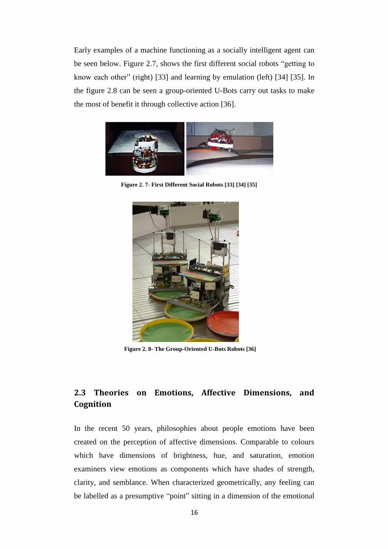
Early examples of a machine functioning as a socially intelligent agent can
be seen below. Figure 2.7, shows the first different social robots “getting to
know each other” (right) [33] and learning by emulation (left) [34] [35]. In
the figure 2.8 can be seen a group-oriented U-Bots carry out tasks to make
the most of benefit it through collective action [36].
2.3 Theories on Emotions, Affective Dimensions, and
Cognition
In the recent 50 years, philosophies about people emotions have been
created on the perception of affective dimensions. Comparable to colours
which have dimensions of brightness, hue, and saturation, emotion
examiners view emotions as components which have shades of strength,
clarity, and semblance. When characterized geometrically, any feeling can
be labelled as a presumptive “point” sitting in a dimension of the emotional
Figure 2. 7- First Different Social Robots [33] [34] [35]
Figure 2. 8- The Group-Oriented U-Bots Robots [36]

17
sphere. Although, emotions are still particular capabilities; some people may
define sadness as similar to sorrow while others may understand sadness as
depression or even indifference. In this interpretation, it isn‘t the actual
emotion that people practice but the nucleus of the emotional experience
that is most researchers seek to label. Existing literature demonstrates that
the importance of assessment must be approved in order to separate between
emotions. A person‘s personal assessment (evaluation) of his or her personal
significance in a situation effects the emotional experience of the person.
Magda Arnold firstly presented “appraisal theory” in 1960 to clarify the
extraction of differentiated emotions, proposes that emotions are the
consequence of a person‘s “appraisal” of a situation and condition through a
specific point in time [37]. Frijda assertions that the basis of the emotion
experience is the sentiment of pleasure or pain with an awareness of
situational sense structure [38]. Davitz and Frijda’s theory says that, it is the
mixture of the pleasure and pain experience with subjectivism which
generates certain stimulant such as the persisting to approach or avoid, wish
to move or stay, or feelings of loss of control [39] [40] [41].
Initial ideas on human sensation group emotions into two scopes valence
and arousal. Earlier effort on the emotional dimensions focused on the
identifying the resemblance of labels of emotions [42], facial expressions
[43], and vocal descriptions of emotional experiences [44]. Recent theories
and studies have presented that the essence of the two-dimensional structure
is insufficient to demonstrate the whole emotional area. Fontaine et al.
represent that at least four dimensions are needed to demonstrate the
resemblances and differences in anthropological emotions. With 144
emotion features used to represent peculiarities of 24 sensation terms3,
Fontaine demonstrated four emotional dimensions as: “evaluation-
pleasantness”, “potency-control”, “activation-arousal”, and
“unpredictability” [21].
3 The 24 emotion terms that Fontaine used to derive the four-dimensional solution are:
anxiety, anger, disgust, being hurt, contempt, contentment, compassion, disgust,
disappointment, fear, guilt, hate, happiness, interest, irritation, jealousy, joy, love,
pleasure, pride, sadness, shame, stress [21].

18
The Four Affective Dimensions
Evaluation-Pleasantness: “Appraisals of intrinsic pleasantness and
goal conduciveness, as well as action tendencies of approach versus
avoidance or moving against (another person or object).” This
dimension designates the positive and negative feelings which are
distinguished by attraction (valence) or loathing of an object, person,
or condition. This distinguishes the experience of pleasant sensations
as different to unpleasant sensations. A pleasant emotion is elicited
by positive valence carrier or objects whereas a negative emotion is
evoked by negatively valence events [21].
Potency-Control: “Appraisals of control, leading to feelings of
power (dominance) or weakness; interpersonal dominance or
submission, including impulses to act or refrain from action.”
Emotions in this aspect comprise vanity, resentment, humiliation as
contrary to sorrow, despair, and shame [21].
Activation-Arousal: “Characterized by sympathetic arousal, such as
rapid heartbeat and readiness for action. It opposes emotions such as
stress, anger, and anxiety to disappointment, contentment, and
compassion.” [21].
Unpredictability: “Appraisals of novelty and unpredictability as
compared with appraisals of expectedness or familiarity.” This
dimension distinguishes astonishment from fondness and emotion of
spontaneity as different from expectancy [21].

19
2.3.1 Facial Action Coding System (FACS)
Various of procedures to measure facial expressions based on physiological
features of the face (image-based methods) have motivated advances in
automatic emotion recognition systems, along with databases developed for
research in facial expression. Ekman and Friesen‘s Facial Action Coding
System (FACS) was established to evaluate and measure human facial
muscle movement. In 1965, FACS is derived from Ekman‘s studies on
facial expressions, which disclosed proof to demonstrate that emotion
expressions are universal4 and cultural [45]. Individual and distinctive
global expressions were detected for disgust, fear, anger, enjoyment, and
sadness [46]. In expanding the Facial Action Coding System, Ekman et. al
observed and studied videotapes of human faces to recognise how changes
in facial muscles result appearance. These facial muscles are named Action
Units (AU) rather than muscles as classification of facial expressions is
based on appearance rather than based on anatomically [20]. FACS
develops prior research which studies emotions in relations with only a few
dimensions5 and evaluates emotions to be distinct from separate situations
[45]. Figure 2.9 shows the demonstration of how the Facial Action Coding
System recognizes muscle groups, named Action Units, responsible for
fluctuating of the appearance of the eyebrows, forehead, eye cover fold, and
upper and lower eyelids.
4 In 1972, Ekman and Friesen extended findings of how people interpret expressions and
discovered “evidence of universality in spontaneous expressions and in expressions that were
deliberately posed” [45]. 5 Early researches in experimental psychology describe emotions as simply positive versus
negative states or as distinctions from states of arousal [63].
Figure 2. 9- Facial Action Coding System [20]

20
2.3.2 FeelTrace: An Instrument to Record Perceived Emotions
Several tools have been developed to record perceived emotions as specified
by the four emotional dimensions. FeelTrace is a tool created on a two-
dimension space (activation and evaluation) which lets an observer to “track
the emotional content of a stimulus as they perceive it over time” [47]. This
tool offers the two emotional dimensions as a rounded area on a computer
screen. Human users of FeelTrace observe a stimulus (e.g. watching a
program on TV, listening to affected melody or displaying strong emotions)
and move a mouse cursor to a place within the circle of emotional area to
label how they realize the incentive as time continues. The measurement of
time is demonstrated indirectly by tracing the position of where the mouse is
in the circle with time measured in milliseconds. Arrangements using the
FeelTrace classification are used to create the labels in the testing described
in this paper. Figure 2.10 is an example of a FeelTrace exhibition while
following a session. The color-coding arrangement allows users to label the
extensity of their emotion. Pure red point to the most negative assessment in
the activation (very active) dimension; pure green point to, when the user is
feeling the most positive evaluation in the activation dimension (very
passive). FeelTrace lets its users to produce annotations of how they observe
specific stimuli at specific points in time. The system has been shown to be
able to perceive changing of emotion over time.
Figure 2. 10- An Example of a Feeltrace Exhibition [47]

21
2.3.3 Automatic Recognition of Facial Emotions Using Feature
Descriptors
From the time when FACS needs manual coding of Action Units by
observers using stop motion video6, the method is time consuming because
over 100 hours of preparation and training is needed to get minimal
competency in human paraphrases. In addition, each minute of video
requires a least possible of an hour to evaluate [48]. The manual procedure
of FACS poses a restriction on this process and encourages researchers in
computer visualization to improve robust and well-organized systems for
automatic recognition of facial expressions. Early endeavour in developing
automatic emotion recognition systems contain those of Kobayashi and
Hara [49], Mase [50], Pantic [51], Cowie [52], and Samal and Iyengar [53].
More recent challenges in this field are in discovering pertinent information
about an image which can be used to create design recognition simulations
that can distribute across other comparable types of images. The state of the
art in 2D face recognition covering Gabor features (expending a set of
Gabor filters with different frequencies and orientations), Local Binary
Pattern (LBP) (using binary pattern vectors to characterize textures of
image), and Edge Orientation Histogram (EOH) (using the orientation angle
of an edge within local image).
Local Binary Pattern, first presented in 1994 and first exploited as an image
texture descriptor on grayscale images, is a widely-used technique in face
recognition [54]. Features specified by the AVEC 2011 Challenge (portion
of the SEMAINE database) utilize a uniform implementation of LBP [52].
These traits were incorporated as part of the research described in the next
chapters.
6 Ekman clarified that “although there are clearly defined relationships between FACS and the underlying facial muscles, FACS is an image-based method. Facial actions are defined by the image changes they produce in video
sequences of face images” [48].

22
Another more recently introduced texture descriptor is Local Phase
Quantization (LPQ), which is a grayscale-level feature that has been
established to be fixed to centrally symmetric blur [55] due to its usage of
the Fourier transform phase. Edge Orientation Histogram is a trait originally
used in hand gesture and motion identification [56]. Since the EOH
algorithm is locally-calculated (the gradient of each pixel is related on its
neighbouring pixels) [56].
2.4 Image Processing Methods
Most of the face recognition methods usually implement pre-processing of
the images prior to feature extraction. Such processes comprise converting
images to grayscale, using an eye recognition algorithm to specify the
position of the eyes (via the Haar-cascade object detector implemented by
OpenCV), and carrying out face detection (via the OpenCV implementation
of the Viola & Jones face detector) to recognize the location of the face so
that it could be cropped out from the remnant of an image. These pre-
processing periods progress the final labelling results as maximum of the
unrelated information of an image is removed. After pre-processing, every
pixel of the grayscale image is stored as an entire number in the range of 0
to 255. Therefore, the image is illustrated as numerical data in a matrix
(respectively each component in the matrix signifies the grayscale intensity
of each pixel in the image) 7
. From the image data, it is possible to achieve
feature extraction to find patterns, and therefore create a model from these
patterns, import it into a learning process, and then test the model on new
data base.
7 In a colour image there are three numeric values in the range of 0 to 255; respectively each numeric value corresponds to the colour intensity of red, green, and blue. For example, given a colour pixel demonstrated as [R, G, B] = [146 120 97], MATLAB‘s rgb2gray function can be used to convert the image from R,G,B to grayscale
value. The algorithm applied is as follows:
[R, G, B] = [146 120 97] Grayscale Intensity = 0.2989*R + 0.5870*G + 0.1140*B
= 0.2989*(146) + 0.5870*(120) + 0.1140*(97) ≈ 125
Consequently, 125 is the numeric value representing a single pixel of an image in grayscale intensity.
23
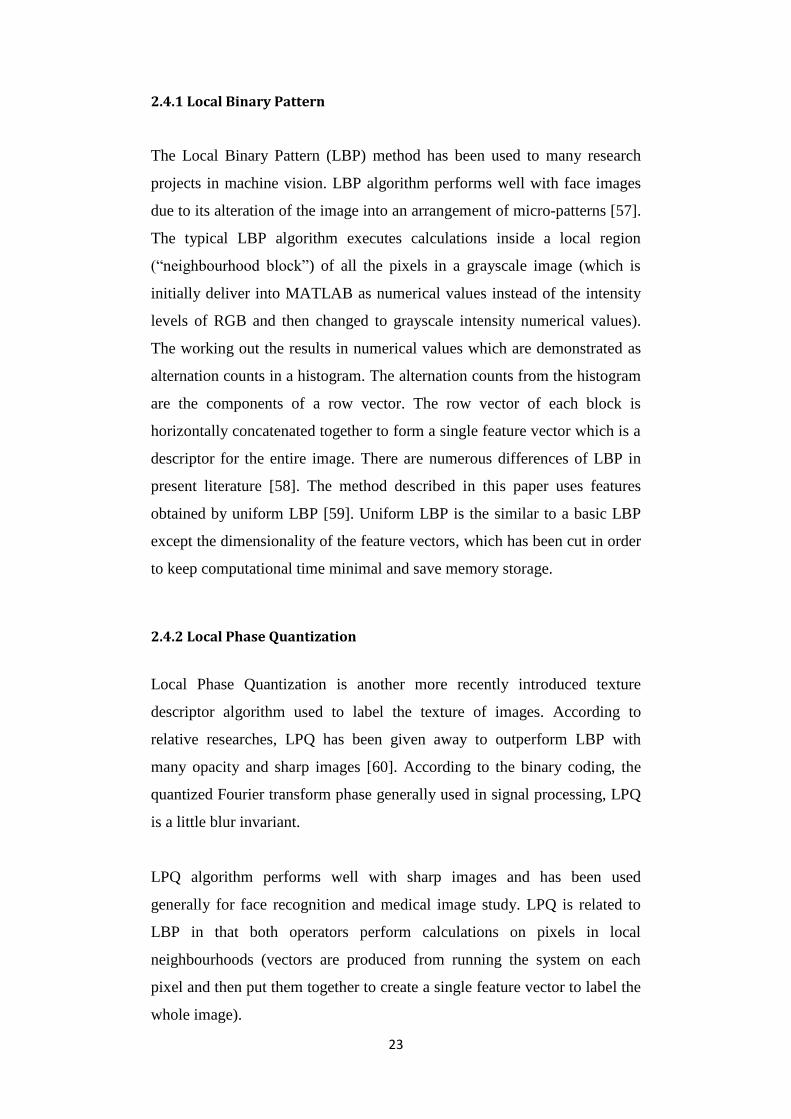
2.4.1 Local Binary Pattern
The Local Binary Pattern (LBP) method has been used to many research
projects in machine vision. LBP algorithm performs well with face images
due to its alteration of the image into an arrangement of micro-patterns [57].
The typical LBP algorithm executes calculations inside a local region
(“neighbourhood block”) of all the pixels in a grayscale image (which is
initially deliver into MATLAB as numerical values instead of the intensity
levels of RGB and then changed to grayscale intensity numerical values).
The working out the results in numerical values which are demonstrated as
alternation counts in a histogram. The alternation counts from the histogram
are the components of a row vector. The row vector of each block is
horizontally concatenated together to form a single feature vector which is a
descriptor for the entire image. There are numerous differences of LBP in
present literature [58]. The method described in this paper uses features
obtained by uniform LBP [59]. Uniform LBP is the similar to a basic LBP
except the dimensionality of the feature vectors, which has been cut in order
to keep computational time minimal and save memory storage.
2.4.2 Local Phase Quantization
Local Phase Quantization is another more recently introduced texture
descriptor algorithm used to label the texture of images. According to
relative researches, LPQ has been given away to outperform LBP with
many opacity and sharp images [60]. According to the binary coding, the
quantized Fourier transform phase generally used in signal processing, LPQ
is a little blur invariant.
LPQ algorithm performs well with sharp images and has been used
generally for face recognition and medical image study. LPQ is related to
LBP in that both operators perform calculations on pixels in local
neighbourhoods (vectors are produced from running the system on each
pixel and then put them together to create a single feature vector to label the
whole image).

24
2.4.3 Edge Orientation Histogram
The Edge Orientation Histogram feature has been presented to perform for
face detection with insignificant databases. This is an advantageous when
considering limitations on processing and computation time and the amount
of memory necessary to create systems from training datasets. Usually, a
large training data samples (e.g. nearly 5,000 data sets) is necessary for a
well performance to obtain good result. However, in practical and in some
real world circumstances, it may not be possible to obtain a large and
enough number of data samples to achieve well performance. Levi et al. has
presented that for frontal faces, EOH features execute as well as the state of
the art whereas using only a few hundred datasets [61]. Typically employed
for hand gesture recognition [56] and object detection [62], EOH features
are created by getting the gradient of particular points of an image, applying
a convolution through Sobel edge detection (which recognizes edges in the
image), and exchanging the orientation of these edges into histograms
(process similar to that of LBP).
2.5 Data Analysis Methodology
2.5.1 The Standard LBP Algorithm Implementation
1. Divide into non-overlapping blocks8.
The grayscale image (each pixel signified as intensity values from 0 to 255)
is divided into non-overlapping square blocks.
In the example on page 26, the block size is 3 pixels by 3 pixels.
In the experiment described in this paper, the LBP features were
derived by dividing the image into blocks
8 Although the standard LBP algorithm does not divide the image into non-overlapping blocks, it is a common
technique used before the LBP operator is performed on every pixel of the image.

25
2. Compare centre pixel inside each block with neighbouring pixels.
A pixel of the image, called the centre pixel, is thresholder against its
neighbouring pixels.
There are 8 neighbouring pixels in a 3 x 3 neighbourhood block.
Pixels along the boundary of the image cannot be used as the centre
pixel, since thresholding must be implemented with all of the pixels
next to the centre pixel.
3. Assign binary values according to comparisons.
If the value of the neighbouring pixel is greater than or equal to the central
pixel, the neighbouring pixel is allocated a value of 1. Otherwise, the
neighbouring pixel is assigned 0.
4. From any optional corner of the block, interlock the numbers in a
counter-clockwise direction as a vector to obtain an 8 bit binary
number. Then convert the binary to decimal value.
In the example on page 27, the upper right corner is chosen. This 0 is
positioned to the right of the binary vector, which is the most significant bit.
Then follows two 0‘s and three 1‘s in a counter- clockwise direction around
the centre pixel. Multiply each weight by powers of two.
5. Add the numbers into a single number.
The 0‘s and 1‘s, now signified as base two values, are added to create one
number. This decimal value signifies the actuarial feature of the single
central pixel.
6. Add “1” to the bin related with this number in a histogram.
The histogram of the frame image represents the frequencies (raw counts) of
each pixel with an exact value (identified as a “bin” value) in the image. For
a histogram express a grayscale image, there are 256 conceivable values
ranging from 0 to 255, so there are 256 bins.
26
7. Repeat all the above steps for all the pixels (except for border pixels).
Each image is represented by a histogram.
8. Exchange the frequency counts of each bin in the histogram into
components of a row vector.
Each bin develops one column in the row vector. The value (total counts)
inside each bin are the components of the row vector.
As there are 256 bins, the row vector has 256 columns. The sum of
the constituents of this vector is the number of centre pixels that
LPB activated on.
As each frame is 640x480 resolution (the resolution used in this
paper) therefore there are 307,200 pixels on each frame image, but
only 304964 pixels are considered and represented in the histogram
since border pixels are not calculated (2236 pixels are not used as
centre pixels). Therefore, in the row vector, the sum of the elements
would be 307,200.
9. Interlock the row vectors of all frames into a single row vector.
The result is the LBP feature vector which labels the overall video creates
on local statistical properties of each pixel.
Each video that is 210 second long and recorded with 25 frames per
second would have 210 × 25 = 5250 frames.
Each frame of a video is an image, so its LBP feature vector would
be 1 by 256.
To represent all the frames of a video, feature vectors for each frame
is vertically concatenated (row 1 represents the first frame, row 2
represents the second frame, etc.). For a 210 second long video
consisting of 5250 frames, the LBP feature is a 5250 by 256
matrixes.

27
Example of the standard Local Binary Pattern (LBP) operator
Step 1: Convert image to grayscale, figure 2.11.
Step 2 and 3: Pick the first centre pixel starting from the left (marked green).
Pixels on the border of the block cannot be used as centre pixels. Then the
next centre pixel would next pixel in the row to the end at the end of the row
The next centre pixel will be chosen from the first pixel from the next row
the Centre pixels are marked in green. Each canter pixel has 8 neighbouring
pixels figure 2.12.
Figure 2. 11- Convert RGB Image to Grayscale Image
Figure 2. 12- Centre Pixel Arrangement along the Image

28
Step 4: Compare the numerical value in the canter pixel with all of its
neighbouring pixels. If the numerical value of the neighbouring pixel is
greater than or equal to that of the canter pixel, mark the neighbouring pixel
with weight value 1. Otherwise, mark it 0 (Figure 2.13).
Figure 2. 13- Comparison of the Centre Pixel with Its Neighbour
Step 5: Transform binary values into a vector by unwinding the matrix in a
clockwise direction. The subsequent new matrix contains only of binary
values. Start at any pixel of this matrix and then it should be followed same
method for the rest (e.g. in this project the right upper corner as shown in
figure 2.14). In a counter clockwise direction, unravel the matrix into a row
vector.
Step 6: Transform the row vector binary value to the decimal value. Add the
numbers transversely into a single number. In a histogram ranging between

29
0 and 255, add a count to the bin (e.g. each number on the x-axis of the
histogram is a “bin” and there are 256 bins, figure 2.14).
Figure 2. 14- Arrangement and Transform Binary Values into a Vector Array
2.5.2 LBP Output on a Single Image
After implementing the LBP method that mention on the last section on the
centre pixel on whole image the resulting image cab be seen on the figure
2.15.
Figure 2. 15- Local Binary Pattern of an Image

30
As previously mention that Pixels on the border of the image cannot be used
as centre pixels therefore the pixel on the border of the image would be
missed and there will be an image with different resolution typically the
new resolution would be:
𝒏𝒆𝒘 𝒓𝒆𝒔𝒐𝒍𝒖𝒕𝒊𝒐𝒏 = (𝒇𝒓𝒂𝒎𝒆 𝒘𝒊𝒕𝒉 − 𝟐) × (𝒇𝒓𝒂𝒎𝒆 𝒉𝒆𝒊𝒈𝒉𝒕 − 𝟐) (2.1)
Therefore the new resolution would be 638 × 478. In order to reform the
resolution to be same as the recorded and initial the border pixel will be
defined to be a 0 for back or 255 for white. In this study the border pixel
which is not considered as centre pixel replaced with the value 0 (black
colour), which can be seen on the figure 2.16
Figure 2. 16- Border Pixel Arraignments in LBP Image
The figure 2.17 shows the process to obtain histograms of a colour images.
Figure 2. 17- All Steps of Obtaining a Histogram of a RGB Image
31
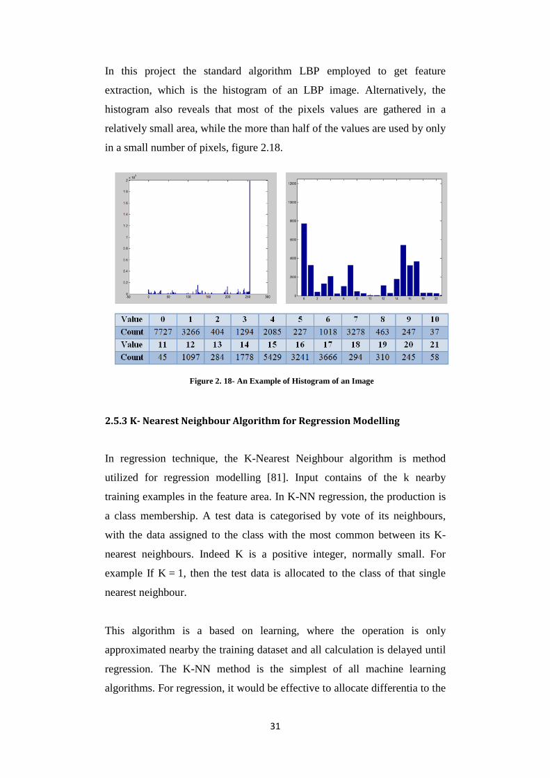
In this project the standard algorithm LBP employed to get feature
extraction, which is the histogram of an LBP image. Alternatively, the
histogram also reveals that most of the pixels values are gathered in a
relatively small area, while the more than half of the values are used by only
in a small number of pixels, figure 2.18.
2.5.3 K- Nearest Neighbour Algorithm for Regression Modelling
In regression technique, the K-Nearest Neighbour algorithm is method
utilized for regression modelling [81]. Input contains of the k nearby
training examples in the feature area. In K-NN regression, the production is
a class membership. A test data is categorised by vote of its neighbours,
with the data assigned to the class with the most common between its K-
nearest neighbours. Indeed K is a positive integer, normally small. For
example If K = 1, then the test data is allocated to the class of that single
nearest neighbour.
This algorithm is a based on learning, where the operation is only
approximated nearby the training dataset and all calculation is delayed until
regression. The K-NN method is the simplest of all machine learning
algorithms. For regression, it would be effective to allocate differentia to the
Figure 2. 18- An Example of Histogram of an Image

32
contributions of the neighbours, so that the closest neighbours play more
roles to the average than the more distant ones [62].
The k-nearest neighbour regression is typically based on distance between a
query point (test sample) and the specified samples (training dataset). There
are many methods available to measure this distance e.g. Euclidean
squared, City-block, and Chebyshev. One of the most common choices to
obtain this distance is well-known as Euclidean. Let 𝑥𝑖 be an input sample
with 𝑃 features ( 𝑥𝑖1 , 𝑥𝑖2 , . . . , 𝑥𝑖𝑝) and 𝑛 be the entire number of input
samples (𝑖 = 1, 2, . . . , 𝑛) and 𝑃 the entire number of features (𝑗 =
1, 2, . . . , 𝑝). Therefore the Euclidean distance between sample
𝑥𝑖 and 𝑥𝑙 (𝑙 = 1, 2, . . . , 𝑛) can be defined as:
𝑑(𝑋𝑖 , 𝑋𝑙) = √(𝑥𝑖1 − 𝑥𝑙1)2 + (𝑥𝑖2 − 𝑥𝑙2)2 + ⋯ (𝑥𝑖𝑃 − 𝑥𝑙𝑃)2 (2.2)
For the K-Nearest Neighbour Predictions, by choosing the value of K, it is
possible to obtain predictions based on the K-NN training dataset.
𝑦 = 1
𝐾 ∑ 𝑦𝑖
𝐾𝑖=1 (2.3)
Where 𝑦𝑖 is the 𝑖 𝑡ℎ case of the training dataset sample and 𝑦 is the
prediction (outcome) of the test sample. In regression problems, K-NN
predictions are founded on a voting system in which the winner is used to
label the query.
2.5.4 Cross-Validation: Evaluating Estimator Performance
Cross validation is a typical confirmation method for measuring the
outcomes of a numerical investigation, which distributes to an independent
dataset. It is usually implemented, wherever the aim is prediction, and the
purpose of using cross validation is estimate how precise predictive system
will implement and perform in practice and real time. In a predictive

33
models, a system is typically given specified a dataset called training
dataset, and a testing dataset against which the system is verified [76] [77].
The aim of this method is to express a dataset to check the system in the
training dataset in order to reduce problems.
Additionally, one of the main reasons that cross validation method used in
this study is that there is a valuable estimator of system performance
therefore, the fault on the test dataset correctly characterise the valuation of
system performance. This is due to that, there is sufficient data accessible
and/or there is a well repartition and a good separation of data into training
and test sets. So a reasonable method to accurately estimate prediction of a
system is to use cross validation.
The holdout method [78] is the simplest variation of cross validation also
called 2-fold cross validation. The dataset is divided into two sets of
datasets, named the training set and the testing set, which both sets are equal
size. Then train one dataset and test on other dataset, followed by training
the second dataset and testing first datasets. The assessment appertain may
be different depending on how to divide the datasets.
K-fold cross validation is that, the dataset is separated into K subsections,
one of the K subsets is chosen for the test dataset and the other K-1 subsets
are used for training dataset. Then the cross validation process repeated K
times, with each of the K subset used once in place validation data. The K
results from the K folds and the average error across all can be computed
and compared. In this method the separation of the data is less important,
which is an advantage of this method as all data tested only once, trained K-
1 times. On the other hand in this method the training algorithm has to be
repeated K times, which funds that it takes K times as much calculation to
create an assessment.

34
2.5.5 Pearson Product-Moment Correlation Coefficient
In measurement, the Pearson Product-moment Correlation Coefficient
(PPMCC) is calculation of the linear correlation between two variables (in
this study between actual labels and predict labels), outcome measurement
is a value between +1 and −1. There are two qualities for each correlation:
strength and direction. The direction indicates that is the correlation either
positive or negative. If factors move in inverse or opposite orders for
example if one variable increases, the other variable decreases, there will be
negative correlation. On the other hand, when two factors have a positive
correlation, it means they move in the same direction. Finally when there is
no relationship between two factors this is called zero correlation [66] [67]
[68]. From the figure 2.19 can be seen that, in the left graph the points lies
close to straight line, which has a positive gradient shows as one variable
increase, the other increase too. The left graph can be seen that the points
lies close to straight line, which has a negative gradient shows as one
variable decrease, the other decrease too. The middle graph shows that no
connection between two variable.
Figure 2. 19- All Type of Correlation Coefficient
However, this method is generally used in the sciences and researches as a
measure of the relationship between two variables .It was established by
Karl Pearson from a relevant thought presented by Francis Galton in the
1880s [66] [67] [68]. There are different types of formula to calculate the
correlation coefficient but the one used in this study is the equation 2.4.
35
𝑟 = 𝑟𝑥𝑦 = 𝑛 ∑ 𝑥𝑖𝑦𝑖− ∑ 𝑥𝑖 ∑ 𝑦𝑖
√𝑛 ∑ 𝑥𝑖2−(∑ 𝑥𝑖)2 √𝑛 ∑ 𝑦𝑖
2−(∑ 𝑦𝑖)2
(2.4)
2.5.6 Discrete Data Methodology on Labels
Whenever talks about analysing a collection data, there is a group of
potential values recorded from an observations or test. There are two diverse
methods to categorize data based on the possible values collected
(Continuous or Discrete data). Discrete data is a data that can be considered
into a classification. Just a limited number of parts or values are possible,
and the value cannot be divided. In this study the result compared in the two
emotion dimension of the FeelTrace in order to better understating and
comparison to evaluate the outcome of the model, therefore the data
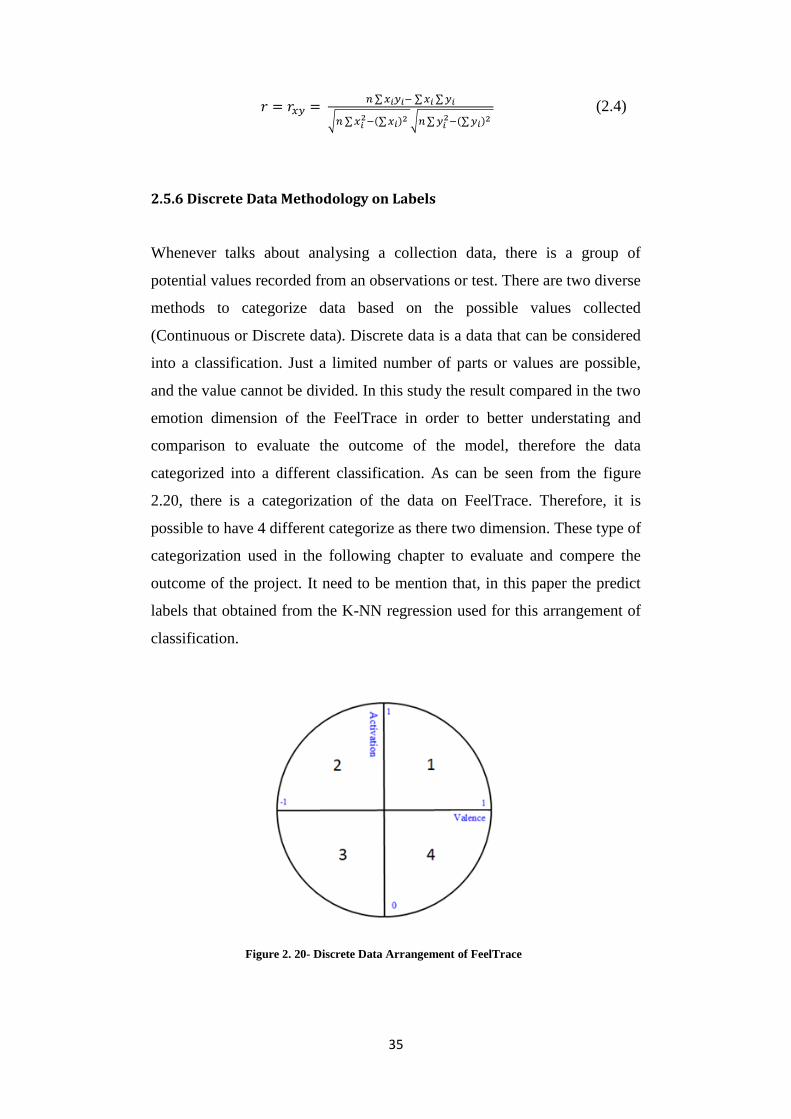
categorized into a different classification. As can be seen from the figure
2.20, there is a categorization of the data on FeelTrace. Therefore, it is
possible to have 4 different categorize as there two dimension. These type of
categorization used in the following chapter to evaluate and compere the
outcome of the project. It need to be mention that, in this paper the predict
labels that obtained from the K-NN regression used for this arrangement of
classification.
Figure 2. 20- Discrete Data Arrangement of FeelTrace
36
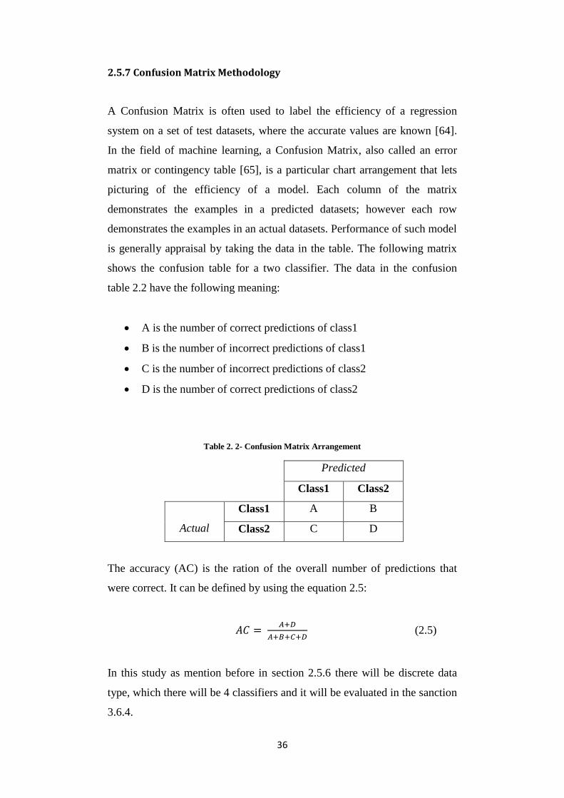
2.5.7 Confusion Matrix Methodology
A Confusion Matrix is often used to label the efficiency of a regression
system on a set of test datasets, where the accurate values are known [64].
In the field of machine learning, a Confusion Matrix, also called an error
matrix or contingency table [65], is a particular chart arrangement that lets
picturing of the efficiency of a model. Each column of the matrix
demonstrates the examples in a predicted datasets; however each row
demonstrates the examples in an actual datasets. Performance of such model
is generally appraisal by taking the data in the table. The following matrix
shows the confusion table for a two classifier. The data in the confusion
table 2.2 have the following meaning:
A is the number of correct predictions of class1
B is the number of incorrect predictions of class1
C is the number of incorrect predictions of class2
D is the number of correct predictions of class2
Table 2. 2- Confusion Matrix Arrangement
Predicted
Class1 Class2
Actual
Class1 A B
Class2 C D
The accuracy (AC) is the ration of the overall number of predictions that
were correct. It can be defined by using the equation 2.5:
𝐴𝐶 = 𝐴+𝐷
𝐴+𝐵+𝐶+𝐷 (2.5)
In this study as mention before in section 2.5.6 there will be discrete data
type, which there will be 4 classifiers and it will be evaluated in the sanction
3.6.4.

37
2.6 Overview of the Classifier Fusion System
The study was conducted in three parts. In order to better understand the
methods that used in the project, all the methods tested on the MATLAB
R2014a in order to use correlation coefficient to validate the results.
Thereafter system implemented on the MATLAB real time simulation with
the live camera. In this project Atlys™ Spartan-6 LX45 FPGA
Development Board used and all testing is carried on this board. Details on
each part described in distinct chapters.
The classification fusion system in this research is generated from the
prediction outputs using LBP features trained and categorised via Support
Vector Machine. Applications was implemented using MATLAB R2014a
with K-NN regression classifier [74] and Xilinx ISE Design Suite 13.2 to
generate VHDL code and download the Hex file to two FPGA board
Atlys™ Spartan-6 FPGA Development Board and Spartan-6 FPGA
Industrial Video Processing Kit. Respectively each output demonstrates the
prediction on each frame of the video and real time camera. At the frame
level, predictions from the regression classifier are used to create a single
regression. The final output is a single prediction. The system erected from
the training dataset is tested on multiple test datasets. Details are described
in the following chapters.
Figure 2. 21- A High-Level Overview of the Classifier Fusion System for Automatic Human
Emotion Recognition

38
This project is the first time that automatic emotional state detection has
been successfully implemented on embedded device (FPGA). To compare
with the other system that mention chapter 1 the system has a capability to
works on real time video inputs with an ability of analysis 30 frames per-
second compare with the Cheng J, Deng Y, Meng H and Wang Z system the
system on the FPGA is producing predict labels on the output 20 times
faster. The model works with real time video capturing this despite that the
Microsoft API emotions detection’s processing capabilities is only on the
single image at the time, while the system on the embedded device is
continues and automatic emotional state detection model.
2.7 Multiple Classifier Fusion System for Emotion Recognition
The concept behind using merger methods to solve regression issues
originates from the thought that there is no solitary method that can achieve
a well result on a wide variety of database. For example, in facial emotion
recognition, although features such as LBP, LPQ, and EOH work well on
particular databases as presented in available studies, each feature does not
necessarily obtain good outcomes when the system created by the training
dataset is employed on totally different image database. A common problem
is that systems are over-fitting to the training database and therefore carry
out poor result when it is examined on new database that has little similarity
with the training database. Some features can be useful for dealing with
situation such as poor lighting, blur or low resolution. Respectively each
feature has its strengths and weaknesses; it is challenging to know which
features are best for certain kinds of images. Even if one feature works well
at predicting the emotions in some frames of a video, it may not perform
well at predicting over all frames of a video. These limitations deliver
motivation to improve systems and methods which incorporate classifier
outputs.

39
3. Facial Expression Recognition System Based on
MATLAB
3.1 Visual Representation of Overall Methodology
This chapter describes and investigates the methodology of automatic
emotional state detection, and classifies the factors that can be optimised.
The effects of changing many system parameters are also presented. The
chapter presents the overall system, and the various system parameters also
are investigated in this chapter of this thesis.
Figure 3. 1- Visual Representation of Overall Methodology
The basic architecture of the automatic emotional state detection system is
shown in figure 3.1 performs the following steps:
The inputs into the merger system are the videos recorded from five
volunteers, which is used to build the system training part, each recorded
twice while watching a 210 second video. Therefore there are 10 training
videos recorded 25 frames per-second (52,500 frames total), for the
MATLAB system first 5 Fold Cross Validation and then 2 fold Cross
Validation implemented, which is well clarified and explained in the
following section 3.6. GTrace employed in order to obtain and build the
training datasets, which is intruded in section 3.5.

40
Local Binary Pattern features are extracted from these videos. Note that
LBP is the most common features extraction that has been used in numerous
emotional state recognition systems.
A K-Nearest Neighbour algorithm is used for the regression due to its
simplicity. At the training phase, features are extracted from image
sequences from the 10 videos. At the testing step, features of the new image
from a camera connected to FPGA are calculated and sent to K-NN for
regression with dimensional emotion labels (e.g. real values for activation
and valence) as the output. As the training set is complete, the entire system
is expected to produce incessant dimensional labels.
This chapter will explained the how the system is implemented on the
MALAB Simulink. To run the model on the MTLAB Simulink environment
it is essential to have camera connected to PC and the install the camera
hardware in the MATLAB Acquisition. To run the model it is necessary to
be in the right folder which the all training data sets are saved and the model
has been created.
The objectives below deliver in this chapter to be followed within the
methods used in last chapter.
Record 10 video from 5 participants
Obtain the feature extraction of 10 video by LBP
Obtain the labels of each frames in the 10 video
Use K-NN on the training dataset
Implementing K-fold Cross Validation and analysis the result
Build the model on MATLAB Simulink
The next section depicts the top-level block diagram employed in order to
perform this chapter objectives mention above.

41
3.2 System Inputs and Output
The inputs into the merger system are the videos recorded from five
volunteers, each recorded twice while watching a five minute video.
Therefore there are 10 training videos recorded 25 frames per-second
(52,500 frames total), for the MATLAB system first 5 videos (26,250
frames) used to create training datasets and second 5 recoded videos (26,250
frames) used as testing datasets (26,250 frames). The videos are read into
MATLAB. Pre-processing details are covered in this chapter. Then feature
extraction is performed on each of these videos using LBP for feature
extraction. Training data built from each of the features is trained via K-NN
to build the regression model. Four kernels and different parameter values
are used to improve prediction accuracy of the models. The decision values
from the best performances are combined and a majority voting scheme is
used for each set of decision values. The same process is use for confidence
measure values. There is a final output: the single prediction from the fusion
of the decision values.
3.3 Data Collection
The data used in the experiment is constructed from five adults human
volunteers (3 males and 2 females, figure 3.2), which is used to build the
system, each person recorded twice while watching a 210 second video. The
video contains 6 different scenarios (relaxation, funny, sadness, scary and
discussing) and tried to cover most of the emotion from the FeelTrace, note
that every volunteer had a dissimilar reaction to each part of the video. The
video was collected from YouTube and it contains audio too, which had
more effect on the participants in order to assist them to feel the situation.
Figure 3. 2- Two Captures of the Video Watched By Participants

42
The details of the parts in the video can be seen in the table 3.1. There are
totally 202 second audio-visual and 8 second gap between each part.
Table 3. 1- Details of the Parts in the Video
Order of Playing Emotion Situation Duration(S)
1 Relax 21
2 Funny 32
3 Sad 59
4 Scary 34
5 disgust 16
6 Relax 40
Each video data collected from Xilinx Spartan-6 LX45 FPGA and camera
sensor, which was connected to it, used and then HDMI output from FPGA
connected to computer afterwards MATLAB Acquisition Toolbox used in
order to receive and save the real time video features from the FPGAs board
to use them for machine learning purpose. The videos are in RGB colour
and for each colour component of a pixel in a frame. Each participant was
recorded from the shoulder above face towards camera while sitting on
chair. It was tried to be natural and real therefore videos recorded in office
with a natural background and in some cases it can be seen that some people
walking and passing in the camera frame. The 10 video recorded contain no
audio as it has no role in this project also it would reduce the volume of the
data therefore data would be processed more rapidly.
Figure 3. 3- Faces of the Participants in the Experiment
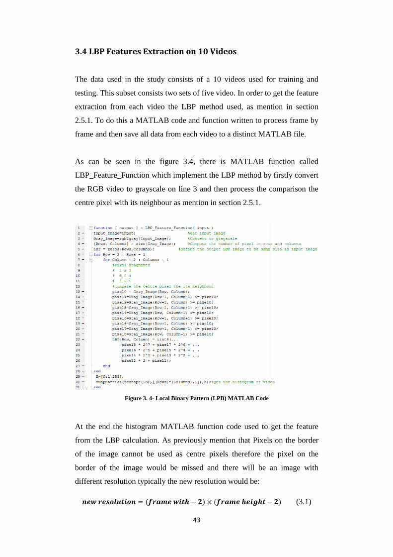
43
3.4 LBP Features Extraction on 10 Videos
The data used in the study consists of a 10 videos used for training and
testing. This subset consists two sets of five video. In order to get the feature
extraction from each video the LBP method used, as mention in section
2.5.1. To do this a MATLAB code and function written to process frame by
frame and then save all data from each video to a distinct MATLAB file.
As can be seen in the figure 3.4, there is MATLAB function called
LBP_Feature_Function which implement the LBP method by firstly convert
the RGB video to grayscale on line 3 and then process the comparison the
centre pixel with its neighbour as mention in section 2.5.1.
Figure 3. 4- Local Binary Pattern (LPB) MATLAB Code
At the end the histogram MATLAB function code used to get the feature
from the LBP calculation. As previously mention that Pixels on the border
of the image cannot be used as centre pixels therefore the pixel on the
border of the image would be missed and there will be an image with
different resolution typically the new resolution would be:
𝒏𝒆𝒘 𝒓𝒆𝒔𝒐𝒍𝒖𝒕𝒊𝒐𝒏 = (𝒇𝒓𝒂𝒎𝒆 𝒘𝒊𝒕𝒉 − 𝟐) × (𝒇𝒓𝒂𝒎𝒆 𝒉𝒆𝒊𝒈𝒉𝒕 − 𝟐) (3.1)

44
Therefore, the new resolution would be 638 × 478. In order to reform the
resolution to be the same as the recorded and initial the border pixel will be
defined to be a 0 for back or 255 for white. In this study the border pixel
which is not considered as centre pixel replaced with the value 0 (black
colour). There are 256 (from 0 to 255) different conceivable intensities in a
grayscale image, and so the histogram displays 256 numbers showing the
distribution of pixels between the 8-bit grayscale numerical values.
After implementing LBP method on the video the MATLAB file contain
their feature has the following details:
1. Number of rows that indicate the frames in the video is 5250.
2. Number of columns that indicate the feature is 256.
Figure 3. 5- An Example of one Frame RGB and LBP View with its Features

45
3.5 Labels of the Two Emotion Dimensions (GTrace)
FeelTrace is used for recording concept of emotion, in terms of two emotion
dimensions – valence (positive to negative) and activation (dynamic to
inert). However, this method of map out is much more general. The
application contains a set of measurements that used to record perceived
emotion linked to impressions figure 3.6. Feeltrace is a labelling implement
for two emotion dimensions, established at Queen's University Belfast. It
lets for the tracking of a perception of emotional state over time, on the two
emotion dimensions activation and evaluation.
The basic form of Gtrace rating is shown in figure 3.7. Left side of the
window, assessor see a video that displays the participant to be rated. On the
other side of window, there is a cursor that assessor can control. It obtains
the form of a chromatic circle, which can be moved only lengthways a
single dimension (left or right). The indicator travels within a space
restricted by a rectangle. The rectangle is divided into equal area within
vertical lines (it may be half, thirds, quarters, etc.). The colour of the
pointer changes as it travels inside the scale. For example, as can be seen in
figure 3.7, in the valence, the pointer is pure red at the strongly negative and
then by moving to the right the colour of the pointer slowly changes and the
green at the positive. This movement leaving bellows after itself, that
expression where it was before.
Figure 3. 6- Feeltrace Exhibition

46
For all 10 videos the labels are worked out form the Gtrace application.
Therefore for each frame there are two labels, activation in range of 0 to 1
and valence in range of -1 to 1, Figure 3.8.
After implementing Gtrace application on the video the MATLAB file
contain their labels have the following details:
1. Number of rows that indicate the frames in the video is 5250.
2. Number of columns that indicate the labels are 2. First column
contains the activation and the second column contains valence.
Figure 3. 7- An Example of Valence Over View in GTrace Environment
Figure 3. 8- Activation and Valence of a Video

47
3.6 Implementing K-Fold Cross Validation
3.6.1 Implementing 5-Fold Cross Validation
As mentioned before cross validation is a typical confirmation method for
measuring the outcomes of a numerical investigation, which distributes to
an independent dataset. It is usually implemented, wherever the aim is
prediction, and the purpose of using cross validation is estimated how
precise predictive system will implement and perform in practice and real
time. In order to implement 5-fold cross validation, the dataset, that contains
10 video features and labels are separated into 5 subsections as follow:
Subsections1: video 1 and 2
Subsections2: video 3 and 4
Subsections3: video 5 and 6
Subsections4: video 7 and 8
Subsections5: video 9 and 10
One of the 5 subsets is chosen for the test dataset and the other 4 subsets are
used for training dataset. Then the cross validation process repeated 5 times,
with each of the 5 subset used once in place validation data. In regression
technique, the K-Nearest Neighbour algorithm (K-NN) is used for three
different K (K= 1, 3 and 5). Therefore the cross validation process repeated
5 times each time for different K, with each of the 5 subset used once in
place validation data. To evaluate the result cross validation methodology,
two types of discreet data and confusion matrix used.
MATLAB codes wrote to implement the 5-fold cross validation on the
features and the labels and the result saved in the MATLAB file.
3.6.2 Implementing 2-Fold Cross Validation
In order to implement 2-fold cross validation, the dataset, that contains 10
video features and labels are separated into 2 subsections. As each

48
participant have been recorded twice thereafter for the 2-fold there will be
odd and even subsection the first recorded dataset of each person put in to
the odd subsection and the second recorded datasets of each person is added
to the even subsection. The 2 subsections as follow:
Subsections odd: video 1, 3, 5, 7 and 9
Subsections even: video 2, 4, 6, 8 and 10
First the odd subset is chosen for the test dataset and the even subset is used
for training dataset. Then the even subset is chosen for the test dataset and
the odd subset is used for training dataset. In regression technique, the K-
Nearest Neighbour algorithm (K-NN) is used for three different K (K= 1, 3
and 5). Therefore the cross validation process repeated 3 times each time
for different K-NN, with each of the 2 subset used once in place validation
data. To evaluate the result cross validation methodology, two types of
discreet data and confusion matrix used.
MATLAB codes wrote to implement the 2-fold cross validation on the
features and the labels and the result saved in the MATLAB file.
3.6.3 Correlation Coefficient Evaluation of 2 and 5 -Fold Cross Validation
In measurement, the Pearson Product-moment Correlation Coefficient is
calculation of the linear correlation between two variables (in this study
between actual labels and predicted labels), outcome measurement is a value
between +1 and −1. There are two qualities for each correlation: strength
and direction. The direction indicates that the correlation is either positive or
negative. If factors move in inverse or opposite orders for example if one
variable increases, the other variable decreases, there will be negative
correlation. On the other hand, when two factors have a positive correlation,
it means they move in the same direction. Finally when there is no
relationship between two factors this is called zero correlation.

49
The outcome of cross validation of the predict labels for 5-Fold Cross
Validation for different K in K-NN (K = 1, 3 and 5) can be seen from the
tables 3.2.
Table 3. 2- Average Correlation Coefficient of 5 Fold Cross Validation
Average Correlation Coefficient of Predict Labels for 5-fold Cross Validation
K Activation Valence
1 0.0226 -0.0137 3 0.0260 -0.0206 5 0.0294 -0.0208
The predict labels of 5-fold cross validation for different K can be seen. The
correlation coefficient average result was obtained, as mention the in the
section 2.5.5, after applying the 5-fold cross validation for all the
subsections. The average activation has positive points therefore all the
points lie close to straight line, which has a positive gradient and shows as
one variable increase in the test datasets, the other points in the predict
labels dataset increase too. On the other hand, The average valance has
negative points therefore all the points lie close to straight line, which is has
a negative gradient and shows as one variable increase in the test datasets,
the other points in the predict labels dataset increase too. However, as can
be seen by increasing the K from 1 to 3 and 3 to 5 the correlation coefficient
for activation increased by 15.04%. Therefore, there is increment of 30.08%
changing the k from 1 to 5 in K-NN. On the other hand, for the valence by
increasing the k from 1 to 3 correlation coefficient increases by 50.36% and
correlation coefficient increases 51.82% for k from 1 to 5.
The outcome of cross validation of the predict labels for 2-Fold Cross
Validation for different K in K-NN (k= 1, 3 and 5) can be seen from the
figure 3.9.

50
Table 3. 3- Average Correlation Coefficient of 2 Fold Cross Validation
Average Correlation Coefficient of Predict Labels for 2-fold Cross Validation
K Activation Valence
1 0.0561 -0.0341
3 0.0713 -0.0362
5 0.0785 -0.0381
The predict labels of 2-fold cross validation for different K can be seen in
table 3.3. The average activation is positive therefore all the points lie close
to straight line, which has a positive gradient and shows as one variable
increase in the test datasets, the other points in the predict labels dataset
increase too. On the other hand, The average valance is negative therefore
all the points lie close to straight line, which has a negative gradient and
shows as one variable increase in the test datasets, the other points in the
predict labels dataset increase too. However, as can be seen by increasing
the k from 1 to 5 the correlation coefficient for activation increased by
39.92%. On the other hand, for the valence by increasing the K from 1 to 5
correlation coefficient increases by 11.73%.
From both methods of the cross validation can be seen that, there is better
correlation coefficient as it gets closer to 1. However, there is less
percentage increment in 2-fold but there is higher correlation coefficient for
this method. In the next sanction the confusion matrix will be analysed.
Figure 3. 9- Predict and Actual Labels of 2 Fold Cross Validation

51
3.6.4 Evaluation of Confusion Matrix of the K-Fold Cross Validation
In comprehension how well the model performed, it is necessary to examine
which frames were correctly and incorrectly predicted. Analysis of the
correctly and wrongly predicted instances reveal that, most of the models
predicted more zeros incorrectly than ones. Furthermore, the final prediction
of the model is designed to be reliable on the decisions of predictions.
Therefore, if the anticipations had been mostly zeros, then the predictions
leaning to be generally zeros when the most of the votes do not consist with
the probability evaluation. In this case the confusion matrix would be
efficient tool to analyse the probability estimation. As mention in section
2.5.7, there is arrangement for the confusion matrix two dimensions, which
contain 4 zones classification. The regression results are used to obtain the
confusion matrix.
3.6.4.1 Confusion Matrix of the 5-Fold Cross Validation
As mentioned before, the predict labels that obtained from the K-NN
regression used for this arrangement of classification and then The
confusion matrix of the result can be seen in table 3.4, from all confusion
matrices, this table is chosen for the best performances of the arguments for
5 fold cross validation for each of the two emotion dimensions. All the
result can be seen in the appendix A.
4 Zones Arrangement
5-Fold Cross Validation k=3
Frames
10500
Predict Labels
1 2 3 4
Actual
Labels
1 85 249 568 805
2 13 28 138 725
3 58 256 505 1221
4 408 1233 1871 2336
Total Correct 2954
Total Wrong 7546
Accuracy % 28.13
Table 3. 4- 4 Zones Confusion Matrix of the 5-Fold Cross Validation

52
As can be seen the best accuracy of the 5 fold cross validation for 4 zone
arrangement, is belong to the K=3 with the accuracy of the 28.13%.
3.6.4.2 Confusion Matrix of the 2-Fold Cross Validation
The following table, from all confusion matrices, is chosen for the best
performances of the arguments for 2 fold cross validation for each of the
two emotion dimensions. All the result can be seen in the appendix A.
As can be seen from the table 3.5 the best accuracy of the 2 fold cross
validation for 4 zone arrangement, is belong to the K=5 with the accuracy of
the 51.28%. In over all, the accuracy of the 4 zones confusion matrix result
can be seen from the table 3.6 the highest accuracy belongs to the 2 fold
cross validation for the K=5.
Table 3. 6- Average Accuracy of Confusion Matrix for Different K
Accuracy %
k 5 Fold 2 Fold
1 27.66 45.82
3 28.13 49.47
5 27.77 51.28
4 Zones Arrangement
2-Fold Cross Validation k=5
Frames
26250
Predict Labels
1 2 3 4
Actual
Labels
1 483 28 353 3407
2 269 16 212 1764
3 463 19 607 4013
4 884 57 1322 12356
Total Correct 13462
Total Wrong 12788
Accuracy % 51.28
Table 3. 5- 4 Zones Confusion Matrix of the 2-Fold Cross Validation

53
3.7 System Overview and Implementation on MATLAB
Simulink
Computer simulation is the order of creating a system of a real physical
model, implementing the system on a computer, and evaluating the
performance output. To comprehend reality and all of a model convolution,
it is essential to create artificial substances and kinetically perform the roles.
Computer simulation is the tantamount of this kind of role and it helps to
determine artificial situations and figurative worlds. One of the main
advantages of employing simulation (MATLAB Simulink) for study and
evaluating of models is that it allows the users to rapidly examine and
evaluate the outcome of complex designs that possibly will be excessively
hard to investigate.
Simulink, established by MATLAB, is a graphical software design
environment for demonstrating, simulating and analysing dynamic models.
Its main communication with a computer is a “graphical block diagramming
tool” and a modifiable of block in its library [69]. In Simulink, it is easy and
simple to represent and create a model and then simulate it demonstrating a
physical model. Systems are demonstrated graphically in Simulink as block.
An extensive collection of blocks is presented for demonstrating numerous
models to the user. Simulink can statistically estimate the solutions to
models that are impossible or are not willing to create and calculate by
hand. The capabilities of the MATLAB Simulink are:
Building the Model
Simulating the Model
Analysing Simulation result
Managing Projects
Connecting to Hardware
In this study MATLAB Simulink used to express the possible actual
efficacy of other situations.

54
3.7.1 Model Design Environment for Demonstrating Emotional State
Detection
As mentioned in the last chapter the highest accuracy belongs to the 2 fold
cross validation with the K=5 for K-Nearest Neighbour. Therefore in the
MATLAB Simulink this method used to create a model. The over view of
the model can be seen from the figure 3.10.
Figure 3. 10- Visual Representation of MATLAB Simulink Model
In this model numerous blocks from the MATLAB used. On the other hand
there are 6 blocks, which created and the MATLAB code written for them
as there was no block for them in the library to meet the model structure. At
the input of the model the block “From Multimedia File” block used to read
the video input and then at its output the video data dived to three RGB
output then the block designed to convert the video to grayscale with the
following parameters;
𝐺𝑟𝑎𝑦𝑠𝑐𝑎𝑙𝑒 = 0.2989 × 𝑅 + 0.5870 × 𝐺 + 0.1140 × 𝐵 (3.2)
From the RGB to grayscale convertor another block designed to obtain the
LBP of the video, which is the same method as used in the last chapters.
Histogram from the LBP result is calculated by using the histogram block
from the library. The training dataset that used in this model got from the
last section using the 2-fold cross validation as the odd subsection used for
test the even subsection used for training. The actual labels also used in this
model to compare with the predict result of the simulation. Also the
FeelTrace image used to display the actual and the predicted labels on it.

55
There is block used to count the frame number to be displayed on the video
and the FeelTrace image. After running the model, it displays the RGB,
grayscale and LBP video followed by showing the histogram of the relevant
frame and finally shows the FeelTrace image with the frame number at
button left corner. The actual label shows in blue and the predict label
displays in red and it is possible to display both output in the same time.
Also correlation block used to display the correlation coefficient between
the actual and predict labels.
In the figure 3.11 can be seen the outputs of MATLAB Simulink Model in
the MATLAB environment the top pictures shows the video image from
RGB to grayscale and the LBP. The left bottom images is the histogram of
the relevant video frame and the left bottom image display the actual and the
predict label on the FeelTrace Image. In this model as the training datasets
include 26250 frames and for each frame there are features also two
dimension label so the model would run very slow to increase the speed of
the model to process the data more faster the training dataset has been
reduced from 26250 to 525 which means that 98% of the data draped and
only 2% of the training datasets used. On the other hand the most time taken
part of the model is, where the LBP block calculated the Local Binary
Pattern of the frame. From the Simulink Profile Report can be seen figure
Figure 3. 11- The Outputs of MATLAB Simulink Model

56
3.12 (full report available in appendix B) each time the model run to process
the LBP it takes 34% of the time taken for the process LBP block and this is
another reason that the model run slower than expected.
Figure 3. 12- Simulink Profile Report for the LBP Block
The model can be modified to be used with camera sensor form the FPGA.
The over view of the model can be seen in the figure3.13.
Figure 3. 13- Visual Representation of MATLAB Simulink Model Real Time
In this model the training dataset that used in last model used, which is 525
frames features and labels used. The large print of both models is available
in appendix B.
3.8 Summery
Within this chapter, the overall model introduced. The system input is
collected from five volunteers. They have been recorded twice from the
shoulder above while watching a 210 second video. These 10 videos are 210
second long with the resolution of 640 × 480 with the frame rate of 25
frames per second. The LBP algorithm used to obtain the features extraction
on each video. On the other hand, the GTrace application used to get the

57
two emotion dimensions labels – valence (positive to negative) and
activation (dynamic to inert). In order to find the best possible method the
K-fold cross validation used and implemented for 2 and 5 fold. The K-
Nearest Neighbour algorithm used for the regression modelling and the
analysis that done on the datasets shows that the most accrue result belongs
to the 5-fold cross validation with K=5 for the K-Nearest Neighbour.
Therefore this method used to build a two system on MATLAB Simulink
the first model was based on training the first five recorded videos data over
the other second recording data to run and displays the predict labels on the
FeelTrace exhibition. The second model built works with real time camera
input from FGPA and trained the data input over the testing datasets to
produce the predict labels displays again on the FeelTrace exhibition. Both
systems perform as expected but both systems work slow due to the LBP
feature extraction as it is not parallel and there will be 1 predict label output
for every 1.05 second, which means that the system is not able to perform
for each frame and while the first frame is processed the other 29 frame
would be last for the real time performance.
58
4. System Implementation on FPGA
4.1 Introduction
Field Programmable Gate Array (FPGA) field carry on to increase
improvement, since its creation by Xilinx in 1984, FPGAs start from
existence plain glue logic chips to really substituting application exact
combined circuits Application Specific Integrated Circuits (ASICs) and also
for processing and controlling applications and signals. FPGA is
semiconductor apparatus, which is built of Configurable Logic Blocks
(CLBs), linked through programmable connection. FPGAs have a capability
to be reprogrammed to designed or desired application subsequently built-
up. This trait separates FPGAs from ASICs, where they are factory-made
for particular design applications. On the other hand, it is possible to have
One Time Programmable (OTP) FPGAs [70]. There are 5 properties and
benefits of productivity of FPGAs.
Performance
The first advantage is that FPGA devises have hardware parallelism;
FPGAs cross the power of Digital Signal Processors (DSPs) by
segregation the consecutive execution per clock cycle.
Time to Market
FPGAs have pliability and fast prototyping, as they can be tested on an
idea and validate it in hardware and do not need to go through the long
procedure of ASIC scheme.
Cost
The expenditure of creating variations to FPGA designs is less when
compare it with ASIC.

59
Reliability
While there are tool provided to program, FPGA is really hard to
carrying out execution. The system is processor based and contains
numerous tools to help for planning tasks and sharing them between
many processes. FPGAs reduce reliability anxieties as used parallel
execution.
Long-Term Maintenance
FPGA devices are upgradable and it does not need the expenditure and
time engaged with ASIC to re-design. As a product or system matures, it
is possible to create useful improvements in short time to re-design the
hardware or changing the design.
However, most emotional state recognition systems have suffered from the
lack of real-time computing ability due to algorithm complexities. It
prevents current systems to be used for real-world applications, especially
for low-cost, low-power consumption and portable systems. Nowadays,
multi-core computer, GPU, and embedded devices have got more power and
the ability for computing acceleration. Many computer vision and pattern
recognition algorithms have been implemented on embedded systems in
real-time based on parallelization in algorithms and hardware processing
architectures. Embedded devices provide a new platform for a real-time
automatic emotional state detection and recognition system.
The objectives below deliver the in this chapter to be followed within the
methods used in last chapter.
Capture images in real time and display on monitor
Obtain the LBP and display on monitor
Use K-NN on the training dataset
Display the predict labels on the monitor

60
The next section depicts the top-level block diagram employed in order to
perform this chapter objectives mentioned above.
4.2 Top-Level Block Diagram
The overall design performed on four dependent functional parts. The first
part is detecting the images from the camera sensor. The second part is
processing the images and implements the LBP in order to get feature
extraction. The third part the classification, using K-NN on the training
dataset. The last part is to display the predicted labels on the screen. A block
diagram and hardware realization of the design can be seen below figures.
Figure 4. 1- A High-Level of Overall Methodology

61
Figure 4. 2 - Visual Representation of Hardware Realization
4.3 Atlys FPGA Board and VmodCAM Camera Sensor
The FPGA board is used to implement the model is Atlys™ Spartan-6
FPGA Development Board [79] along with a VmodCAM Stereo Camera
Module [80]. It use Xilinx Spartan-6LX45 FPGA and has 128 Mbyte DDR2
RAM with 16-bit wide data; more Features and the input/output ports can be
seen in figure 4.3. The Atlys™ board is intended for real time video
processing.
Figure 4. 3- Ports Layout of the Atlys Spartan-6 FPGA Board [71]
The VmodCAM is an additive device to the Atlys board. The Spartan-
6LX45 FPGA sends commands and resolution settings to the VmodCAM
through the I2C line. It contains a selection of clock, image colour and data

62
settings. However there are 2 cameras built in the VmodCAM, only 1
employed for the project. The data that sent back to the FPGA board is in
RGB or YCrCb format. The output table formats are specified in table 4.1.
In order to use and connect the VmodCAM with the Atlys FPGA board a
module, which created for the Atlys™ Spartan-6 FPGA Development
Board, used in this study [72]. This model designed for both camera sensors
on the VmodCAM, FPGA drives the HDMI output for both cameras. This
model created on the Xilinx ISE Design Tools in VHDL and it has been
modified to suit the project specification. The Digilent design code offers
two different configurations with the VmodCAM. The first configuration is
intended to produce the HDMI output with the maximum resolution (1600 x
1200 pixels); the second configuration is intended to produce VGA
(640x480 pixels ) resolution with HDMI output. As mention in last chapter
the low resolution would have faster process on the LBP feature extraction.
Therefore the VGA resolution is more appropriate to the project, so it is
determined that the VGA resolution used to build the project on.
4.4 RGB to YCrCb (Y or Grayscale)
The VGA resolution bit file can be downloaded to the Atlys Board via
Digilent Adept software. When the programing file loaded to the board, the
Table 4. 1- VmodCAM Output Formats [80]

63
output images from the camera sensor can be seen on the monitor through
the HDMI port. In order to implement LBP feature extraction algorithm on
the images, the Digilent code needed to be modified. As mentioned in last
chapters the first steps are to convert the RGB image to Grayscale image.
After some study of the Digilent’s provided code, the subsequent data is
specified. There are two camera sensors in the VmodCAM which called
them the code “CAM_A” and “CAM_B”. The output from the camera for
each pixel is 16-bits. These 16-bit pixels are in RGB565 format, table 4.1.
The most significant 5 bits is related to the Red part, the 6 inner bits are
related to the Green part, and 5 least significant bits belong to the Blue part.
The subsequent step is accumulating the pixel value to the DDR2 memory.
Finally, the last step in the model is to execute a section “DVI transmitter”
for showing the pixels value on the monitor via HDMI port.
In order to convert RGB to Grayscale, a Xilinx logiCORE IP RGB to
YCrCb colour-Space Converter v3.0 used and fitted in the design. It is a
basic 3 by 3 matrix multiplier changing three participation colours, which is
24 bits, to three output samples, which is 24 bit, (8 bits for each elements Y,
Cr and Cb) only in one clock period. In this project only the 8 bits value of
Y used, which correspond for grayscale level of the input RBG. To produce
grayscale value or Y. Based on these project, the standards for coefficients
CA and CB were specified in chapter 2, such that:
Y = CA × R + (1 − CA − CB) × G + CB × B (4.1)
Where the CA = 0.2989 and the CB = 0.1140 and the green colour would
multiply with 0.5871. Therefore the over view of the convertor can be seen
in figure 4.4.

64
Figure 4. 4- Xilinx LogiCORE IP RGB to YCrCb Colour-Space Converter V3.0
In the IP generator can be seen that there are 23 bit video data in regarding
the RGB value and horizontal and vertical counter of the video to indicate
the pixel in the two dimensions. Also there is one pit specified for whenever
the pixel is ready called ACRIVE_VIDEO_IN. Also there is clock input and
reset included in the IP. On the other hand there is video data with 23 bits,
which only the 8 least significant bits that correspond to the Y or grayscale
level used. Also there is ACRIVE_VIDEO_OUT used to indicate whenever
the output is ready also the horizontal and vertical pixel counter are in the
output. The conversion of RGB to grayscale can be seen in figure 4.5.
Figure 4. 5- RGB to Grayscale Conversion on FPGA
RGB to Grayscale

65
4.5 Implementing LBP on FPGA and Obtaining the Features
As mention before, the next step after converting the RGB video data to
grayscale is to implement LBP method on the data. In the MATLAB
Simulink as there was all frame pixels available therefore it was possible to
process LBP on whole image in blocks of 3x3 pixels. On the other hand as
there is not enough RAM memory on FGPA to save all pixels of a single
frame also aimed to have parallel LBP output therefore, a row vector used in
the code to save 1283, which is equal to first two rows pixel values pulse
three pixels from third row as can be seen in table 4.2.
Table 4. 2- Pixels Arrangement In Order To Obtain the LBP
Therefore, it is required to wait until 1283 pixels value to be processed. As
soon as the pixel 1283 generated then there will a block 3x3 available to
process LBP algorithm. For the rest of pixels the pixel value will over
follow and replaced with the pixel after itself. This process would carry the
same way for all pixels to the end. However, as for the camera sensor
capture 30 frames per second with the resolution of 640 × 480 so each
pixel takes 108.51ns to be executed therefore, there will be a delay of
139.21µs to produce the LBP pixel value. In order to wait for 1283 pixels to
be ready a delay generated to do this. It would count the horizontal and
vertical pixels and all the RGB data for all 1283 pixels would be saved in an
array to be accessed in LBP processor and as soon as the third pixel in the
third row ready the IP Core will executed and will calculate and release the
value of the pixel to the output. For the rest of the pixels this process would
be carried the same way for all pixels to the end.
1 2 3 ........................................................... 639 640
641 642 643 ........................................................... 1279 1280
1281 1282 1283 ........................................................... 1919 1920
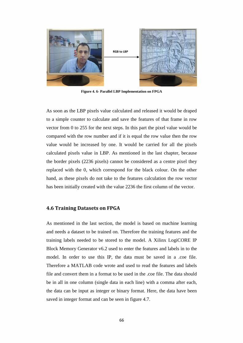
66
Figure 4. 6- Parallel LBP Implementation on FPGA
As soon as the LBP pixels value calculated and released it would be draped
to a simple counter to calculate and save the features of that frame in row
vector from 0 to 255 for the next steps. In this part the pixel value would be
compared with the row number and if it is equal the row value then the row
value would be increased by one. It would be carried for all the pixels
calculated pixels value in LBP. As mentioned in the last chapter, because
the border pixels (2236 pixels) cannot be considered as a centre pixel they
replaced with the 0, which correspond for the black colour. On the other
hand, as these pixels do not take to the features calculation the row vector
has been initially created with the value 2236 the first column of the vector.
4.6 Training Datasets on FPGA
As mentioned in the last section, the model is based on machine learning
and needs a dataset to be trained on. Therefore the training features and the
training labels needed to be stored to the model. A Xilinx LogiCORE IP
Block Memory Generator v6.2 used to enter the features and labels in to the
model. In order to use this IP, the data must be saved in a .coe file.
Therefore a MATLAB code wrote and used to read the features and labels
file and convert them in a format to be used in the .coe file. The data should
be in all in one column (single data in each line) with a comma after each,
the data can be input as integer or binary format. Here, the data have been
saved in integer format and can be seen in figure 4.7.
RGB to LBP

67
Figure 4. 7- All Dataset (Features, Labels) Saved In .Coe File
Windows Notepad used to save the data in .coe. However the biggest data in
the features training dataset is 51256 in decimal to represent it in the Block
Memory Generator IPCore 16 bits width needed, which will limit and
reduce the length of the data that can be used, which means that with the
data of 16 bits there will be only 9999 lines available. However to represent
the feature in the .coe file it is possible to have only on data in each line on
the other hand, as every 256 lines in the file represent for one frame features
and only 9999 lines available therefore in overall only 390 frames of data
can be loaded to the IP. This is a disadvantage, as it will limit the model
training datasets and will drop the accuracy of the output.
Figure 4. 8- Xilinx LogiCORE IP Block Memory Generator V6.2

68
It can be seen in figure 4.8, that Block Memory Generator IP read the data
out per each clock cycle line by line by simple counter. However, as can be
seen in figure 4.7, the training labels are divided in to two separate .coe
files. On the other hand as the labels will display on the top right corner of
the monitor to represent the FeelTrace image with resolution of 100 × 100,
the activation and valence have been transferred to positive (for Valence)
and the range of 0 to 100 to be easily display on the monitor.
4.7 Implementing K-NN Algorithm on the FPGA
As mentioned in last chapter, the K-NN algorithm used as modelling
method, the same algorithm is used to implement the model in the FPGA.
The K-NN equation contains the maths operation (power of 2 and the
Square Root). On the other hand in Xilinx ISE Design Suite there is no
direct command to operate these two operations, even there is no command
to multiply two numbers together. Therefore, to implement the K-NN
algorithm another two logiCORE IP Cores used.
𝑑(𝑋𝑖 , 𝑋𝑙) = √(𝑥𝑖1 − 𝑥𝑙1)2 + (𝑥𝑖2 − 𝑥𝑙2)2 + ⋯ (𝑥𝑖𝑃 − 𝑥𝑙𝑃)2 (4.2)
As can been seen from the equation 4.2 to obtain and calculate the distance
of test feature from training feature datasets so the difference between each
feature element must be squared or multiple with itself. Therefore the
Xilinx logiCORE IP Multiplier v11.2 applied to the model. In this IP the
maximum width of each number can be 18 bit unsigned data, which is
enough for the distance calculation.

69
Figure 4. 9- Xilinx LogiCORE IP Multiplier V11.2
Also after squaring the data, in order to get the distance, the square root has
to be done on the data. However, there is no direct command for square
root in the Xilinx ISE Design Suite therefore, Xilinx LogiCORE IP
CORDIC v4.0, which is available in the IP CORE Generator & Architecture
Wizard, used.
Figure 4. 10- Xilinx LogiCORE IP Cordic V.4
As can be seen from the figure 4.10 the CORDIC IP can be used for
different mathematic operations in this project only the square root used.
The maximum bit can be used for input and output range of 8 to 48 bits, in
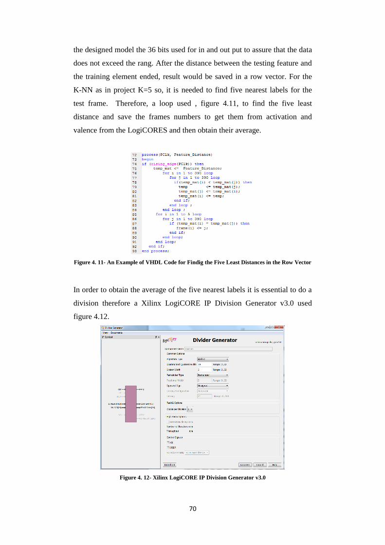
70
the designed model the 36 bits used for in and out put to assure that the data
does not exceed the rang. After the distance between the testing feature and
the training element ended, result would be saved in a row vector. For the
K-NN as in project K=5 so, it is needed to find five nearest labels for the
test frame. Therefore, a loop used , figure 4.11, to find the five least
distance and save the frames numbers to get them from activation and
valence from the LogiCORES and then obtain their average.
Figure 4. 11- An Example of VHDL Code for Findig the Five Least Distances in the Row Vector
In order to obtain the average of the five nearest labels it is essential to do a
division therefore a Xilinx LogiCORE IP Division Generator v3.0 used
figure 4.12.
Figure 4. 12- Xilinx LogiCORE IP Division Generator v3.0

71
The input of this IP would be an unsigned 19 bit vector with a divisor bit of
3 bit. Each of these LogiCORES executes with an input clock for this
project designed so that they work on the rising edge of the clock input.
4.8 Implementing, Compiling and Simulating the Model
In order to implement the model and test it a new project created on the
Xilinx ISE. All the above methods mentioned used to create a simulation.
This code is designed to read a testing and training datasets and create a
predict labels for each frames and save them in a text file. The result of the
predict labels for average correlation coefficient and the 4 zones of the
confusion matrices for 5 fold cross validation can be seen in the table 4.3
and 4.4.
Table 4. 3- Average Correlation Coefficient of Xilinx Simulation
Predict Labels 2-fold cross validation for K=5 on Xilinx
Simulation Activation Valence
Average
Correlation 0.0539 -0.0698
Table 4. 4- 4 Zones Confusion Matrix of the 2-Fold Cross Validation Xilinx Simulation
4 Zones Arrangement
2-Fold Cross Validation k=5 Xilinx simulation
Frames
390
Predict Labels
1 2 3 4
Actual
Labels
1 4 1 6 55
2 3 1 4 27
3 5 1 9 62
4 19 2 24 171
Total Correct 185
Total Wrong 205
Accuracy % 47.44

72
As can be seen from table 4.3, compare with MATLAB, the average cross
validation for activation is reduced by 31.34% and for valence is reduced by
45.42% also from table 4.4, accuracy of the predict labels reduced compare
with MATLAB design 8.45%. It is due to the lower training datasets that
was possible to be used in the VHDL code.
The outcome of cross validation of the predict labels and actual labels graph
for 2-Fold Cross Validation for different K in K-NN (k= 1, 3 and 5) can be
seen from the figure 4.13.
4.9 Real-time GUI
After that K-NN implemented on the testing and training datasets the
activation and valence needed to be displayed. It is necessary to mention
that, the camera sensor capture 30 frames per second, therefore for every
second there will be 30 predict labels on the output, which would be too fast
to see and follow. Therefore in order to see the predict label only one frame
out of 30 frames would be tested on the training datasets, in order to see the
predict labels on the monitor. Therefore for every second there will be an
output, which is the predict label. When the model bit file downloaded to
the FPGA board the camera output, which is the live camera, can be seen on
the monitor, the code has been modified to display the two dimensional
FeelTrace axis on the top right corner of the monitor whit a white
Figure 4. 13- Predict and Actual Labels of 2 Fold Cross Validation

73
background with the resolution of 100 × 100 with blue axis the horizontal
axes indicate valence and the vertical axes indicate the activation. The
predict label will be displayed in red colour; a box 3 × 3 included 9 pixels.
One of the switches in the board used in order to switch between both RGB
and LBP view output, figure 4.14.
Figure 4. 14- Parallel LBP and K-NN Implementation on FPGA
4.10 Speed comparison between the MATLAB Simulink and
FPGA implementation
As mentioned in chapter 3 the model on the MATLAB Simulink run slow
because of execution of the LBP algorithm. As can be seen from the
Simulink Profile Report the time taken for the model to release and predict
label to the output is 1.05 second, which means that the system process each
0.95 frame for every second. On the other hand as mentioned in this chapter
the FPGA execute 30 frames per second and display the predict label on the
screen, therefore the model on the FPGA is 30 times faster than on the
MATLAB Simulink, Figure 4.15.

74
4.11 Summery
Within this chapter, the system and method that used to build the model in
MATLAB Simulink in the last chapter used to create a model to automatic
emotional state detection. To do this the Atlys™ Spartan-6 FPGA
development board and VmodCAM stereo camera module used. The VHDL
code for the camera is provided from the Digilent, this code only generates
the pixels value to be displayed on the monitor. In order to build the model,
the Digilent code used and modified a lot to meet the system requirement.
To do this, analyses done on the provided code to understand each elements
of the code and then three Xilinx LogiCORE IP Block Memory Generator
v6.2 used to add the training datasets the disadvantage of this LogiCORE is
that only 390 frames of data can be used due to its limitation of data input.
And then another 4 LogiCOREs used to build the parallel LBP algorithm
and K-NN on the system.
On the other hand a test bench created to analyse the output on the model.
The accuracy of the predict labels 47.44%; compare with the MATLAB
version the accuracy is draped by 8.45% due to the lower testing datasets.
In order to display the two dimensional FeelTrace an axis on the top right
corner of the monitor displays, which has a white background with the
resolution of 100 × 100 with blue axis the horizontal axes indicate valence
and the vertical axes indicate the activation. The predict label will be
0.95
30
0
5
10
15
20
25
30
35
Matlab Time-Cost 1s FPGA Time-Cost 1s
Fram
es
Figure 4. 15- Comparing Speed of MATLAB and FPGA

75
displayed in red colour; a box 3 × 3 bock of pixels included 9 pixels. One
of the switches in the board used in order to switch between both RGB and
LBP view output.

76
5. Conclusion and Future Work
5.1 Conclusion
The objective of this study was to appraise the efficiency of regression
methods for an automatic emotional state detection and analysis on
embedded devices to be done on human emotion recognition from live
camera. A model designed to process emotional state using a collection of
datasets for training and testing. These databases came from five recoded
video from five participants each has been recorded twice. The Local Binary
Pattern (LBP) method implemented to get the features extraction of each
video (frame by frame) by using MATLAB coding. The labels database for
each frame of the two emotions (Activity and Valence) created using the
FeelTrace definition and GTrace application, which is an application to
record apperception emotions using a scoring system. In regression
modelling technique, the K-Nearest Neighbour (K-NN) algorithm is a
method utilized for regression used, then a model designed and tested in
MATLAB with 2 and 5 fold cross validation with K-NN regression for
different K value (1, 3 and 5). As seen in the chapter 3 the best result
belongs to the 2-fold cross validation with K=5 for the K-NN.
In this study the MATLAB used to test the model and find the best possible
method that can be implemented on the available FPGA. A collection of
video needed to be recorded to build the model database and it has to get
from the FPGA sensor camera (VmodCAM). The biggest challenge on this
project was how to get out the video data from FPGA and save them, on the
other hand, there is only 128 Mbyte DDR2 RAM available on the FPGA
board so there was a limitation to save the video data. So the three different
ways implemented and tested on the two different boards.
1. Receive and save the data in MATLAB Simulink via UART
(Universal Asynchronous Receiver/Transmitter) available on the
board.

77
2. Save data on SD card implement and test on Xilinx Spartan-6 FPGA
Industrial Video Processing Kit
3. Connecting the HDMI output to computer and using MATLAB
Acquisition application to record the video.
And finally the third option found the best way to save the data.
To build a model in VHDL code the Xilinx Spartan-6LX45 FPGA used.
The code that Digilent provided has been used and modified a lot to meet
the project specification. On this way many different Xilinx LogiCORE IP
used. The output of the model would be displayed on the right top corner of
a monitor with the participant live video. There is an option to view the
RGB of LBP view format of the video via a switch designed for that. It is
possible to switch between this two at any time. As mention in chapter three
and four the best accuracy achieved in MATLAB Simulink are 51.28% and
the Xilinx simulation 47.44%.
5.2 Further Work
The system on the embedded device is 47.77%. It can be improved by using
different features extraction techniques such as LPQ, EOH or different
regression modelling methods such as SVM. Regression classifier fusion
systems, although difficult to design, have proven potential to overcome the
problems facing human emotion research today. Perhaps someday, with
even stronger image features, more powerful computation capacities, and
higher quality visual data, it will be possible to build automatic human
emotion recognition systems with nearly perfect accuracy. The effect of
accurate emotion recognition systems are endless; from more intelligent
social robots to better ways to evaluate persons in states of pain or mental
distress, advancements in affective computing have tremendous real-world
applications. Presently, research in this exciting machine learning field is
growing in demand for both industry and academia. The results produced by

78
this simple fusion system for human facial emotion recognition from video
tell us that the future for affective computing will be a fascinating.

79
References
[1] P. Ekman, Universal facial expressions of emotion, California Mental
Health Research Digest 8 (1970) 151-158.
[2] N. Fragopanagos, J. G. Taylor, Emotion recognition in human-computer
interaction, Neural Networks 18 (2005) 389-405.
[3] A. J. Calder, A. W. Young, D. I. Perrett, N. L. Etco, D. Rowland,
Categorical perception of morphed facial expressions, Visual Cognition 3
(1996) 81-117.
[4] B. de Gelder, J.-P. Teunisse, P. J. Benson, Categorical perception of
facial expressions: categories and their internal structure, Cognition and
Emotion 11 (1) (1997) 1-23.
[5] Miwa H., Itoh K., Matsumoto M., Zecca M., Takanobu H., Rocella S.,
Carrozza M.C., Dario P., Takanishi A. (2004), Effective emotional
expressions with expression humanoid robot WE-4RII: integration of
humanoid robot hand RCH-1, Proceedings of IEEE/RSJ International
Conference on Intelligent Robots and Systems, 3: 2203-2208.
[6] C. Darwin, edited by F. Darwin, “The Expression of the Emotions in
Man and Animals,” 2nd
edition, J. Murray, London, 1904.
[7] Picard R. (1997), Affective computing, MIT Press, Cambridge.
[8] Kaliouby, R and Robinson, P. (2005). Real-time inference of complex
mental states from facial expressions and head gestures, Real-Time Vision
for Human-Computer Interaction, Springer, 181-200.
[9] Yang S., Bhanu B. (2012), Understanding discrete facial expressions in
video using an emotion avatar image,IEEE Transactions on Systems, Man,
and Cybernetics, Part B: Cybernetics, vol. PP, no.99:1-13.(online version).

80
[10] Meng H. and Bianchi-Berthouze N. (2011), Naturalistic affective
expression classification by a multi-stage approach based on Hidden
Markov Models. 1st International Audio/Visual Emotion Challenge and
Workshop (AVEC 2011), LNCS 6975: 378-387.
[11] Meng, H., Romera-Paredes, B., Bianchi-Berthouze, N. (2011). Emotion
recognition by two view SVM_2K classifier on dynamic facial expression
features. Proceedings of the 9th IEEE International Conference on Face and
Gesture Recognition (FG'11), FERA 2011-Workshop on Facial Expression
Recognition and Analysis Challenge, LNCS 6974: 854-859.
[12] Descartes, Rene. Passions de l’Ame (The Passions of the Soule),
translated from French into English (translator unknown). London: printed
for A.C. and sold by J. Martin and J. Ridley, 1650.
[13] Merriam-Webster (2004). The Merriam-Webster dictionary (11th ed.).
Springfield, MA: Author.
[14] Hume, D. Emotions and Moods. Organizational Behavior, 258-297.
[15] Schmitter, Amy M. "17th and 18th Century Theories of Emotions."
Stanford Encyclopedia of Philosophy. Edited by Edward N. Zalta. 2009.
http://plato.stanford.edu/archives/win2010/entries/emotions-17th18th/
(accessed November 25, 2014).
[16] Scherer, Klaus R. "What are emotions? And how can they be
measured?" Social Science Information (SAGE Publications) 44, no. 4
(2005): 695-729.
[17] Darwin, Charles. The Expression of Emotions in Man and Animals.
London: Murray, 1872: 13
[18] Darwin, Charles. The Expression of Emotions in Man and Animals.
London: Murray, 1872: 180

81
[19] Bell, Charles. Essays on the anatomy of the expression in painting.
(Later titled "Essays on the anatomy and philosophy of the expression"
(1824) and "The anatomy and philosophy of expression as connected with
the fine arts" (1893). London: Murray, 1806.
[20] Ekman, Paul, Wallace V. Friesen, and Joseph C. Hager. "Facial Action
Coding System The Manual." Facial Action Coding System. 2002.
http://face-and-emotion.com/dataface/facs/manual/TitlePage.html (accessed
November 23, 2014).
[21] Fontaine, R. J., Klaus R. Scherer, Etienne B. Roesch, and Phoebe C.
Ellsworth. "The World of Emotions is Not Two-Dimensional."
Physiological Science (Association for Psychological Science) 18, no. 12
(December 2007): 1050-1057.
[22] Davidson, Richard J., Paul Ekman, Clifford D. Saron, Joseph A.
Senulis, and Wallace V. Friesen. "Approach-Withdrawal and Cerebral
Asymmetry: Emotional Expression and Brain Physiology I." Journal of
Personality and Social Psychology (Americal Psychological Association)
58, no. 2 (1990): 330-341.
[23] Stemmler, G. "Methodological considerations in the
psychophysiological study of emotion." Edited by R. J. Davidson, K. R.
Scherer and H. Goldsmith. Handbook of affective sciences, 2003: 225-255.
[24] Harrigan, J., R. Rosenthal, and K. R. Scherer. The New Handbook of
Methods in Nonverbal Behavior Research. Oxforde: Oxford University
Press, 2005.
[25] Picard, Rosalind W. Affective Computing. Cambridge, Massachusetts:
MIT Press, 1997.
82
[26] Picard, Rosalind W., and Jonathan Klein. "Computers that Recognise
and Respond to User: Theoretical and Practical Implications." Interacting
with Computers (14), 2002: 141-169.
[27] Picard, Rosalind W. "Toward Computers That Recognize and Respond
to User Emotion." IBM Systems Journal (39), 2000: 705-719.
[28] Picard, Rosalind W. Towards Machines With Emotional Intelligence.
Paper, Cambridge, Massachusetts: MIT Media Laboratory, 2000, 705–719.
[29] Healey, Jennifer A., and Rosalind W. Picard. "Detecting Stress During
Real-World Driving Tasks Using Physiological Sensors." IEEE
Transactions on Intelligent Transportation Systems, 2005.
[30] Predinger, Helmut, and Mitsuru Ishizuka. "The Empathic Companion:
A Character-based Interface that Addresses Users' Affective States."
Applied Artificial Intelligence Journal, 2005.
[31] Lisetti, C., F. Nasoz, C. LeRouge, O. Ozyer, and K. Alvarez.
"Developing multimodal intelligent affective interfaces for tele-home health
care." International Journal of Human-Computer Studies 59, no. 1-2 (2003):
245-255.
[32] Fong, Terrence, Illah Nourbakhsh, and Kerstin Dautenhahn. A Survey
of Socially Interactive Robots: Concepts, Design, and Applications. Paper,
The Robotics Institute, Carnegie Mellon University, Pittsburgh,
Pennsylvania: Carnegie Mellon University, 2002.
[33] K. Dautenhahn, Getting to know each other artificial social intelligence
for autonomous robots, Robotics and Autonomous Systems 16 (1995).
Conference, 1999.
[34] A. Billard and K. Dautenhahn, Grounding communication in situated,
social robots, in:

83
Proceedings of Towards Intelligent Mobile Robots Conference, Report
UMCS-97-9-1, Department of Computer Science, Manchester University,
1997.
[35] A. Billard and K. Dautenhahn, Grounding communication in
autonomous robots: an experimental study, Robotics and Autonomous
Systems 24 (1-2) (1998).
[36] University of the West of England, Intelligent Systems Laboratory. U-
Bot. http://www.ias.uwe.ac.uk/Ant%20Lab/ant_lab2.htm (accessed August
20, 2014).
[37] Arnold, M. B. "Emotion and Personality." Psychological Aspects
(Columbia University Press) 1 (1960).
[38] Frijda, Nico H. "The Laws of Emotion." Edited by W. Gerrod Parrott.
Emotions in Social Psychology (Psychology Press), 2001: 59.
[39] Davitz, J. R. The language of emotion. New York: Academic Press,
1969.
[40] Frijda, N. H. The emotions. London: Cambridge University Press,
1986.
[41] Frijda, Nico H. "Emotions, cognitive structure and action tendency."
Cognition and Emotion, 1987: 115-144.
42] Fontaine, J. R. J., Y. H. Poortinga, B. Setiadi, and S. M. Suprapti.
"Cognitive structure of emotion in terms of Indonesia and The Netherlands."
Cognition and Emotion 16 (2002): 61-86.
[43] Schlosberg, H. "The description of facial expressions in terms of two
dimensions." Journal of Experimental Psychology 44 (1952): 229-237.

84
[44] Scherer, Klaus R. "Toward a Concept of "Modal Emotions"." Edited by
Paul Ekman and R. J. Davidson. The nature of emotion: Fundamental
questions (Oxford University Press), 1994: 25-31.
[45] Ekman, Paul. "Facial Expression and Emotion." American
Psychologist, 1993: 384-392.
[46] Ekman, Paul. "Facial Expression of Emotion: New findings, new
questions." Psychological Science 3 (1992): 34-38.
[47] Cowie, Roddy, Ellen Douglas-Cowie, Susie Savvidou, Edelle
McMahon, Martin Sawey, and Marc Schroeder. "'FEELTRACE': An
instrument for recording perceived emotion in real time." Proceedings of
ISCA Workshop on Speech and Emotion, 2000: 19-24.
[48] Donato, Gianluca, Marian Stewart Bartlett, Joseph C. Hager, Paul
Ekman, and Terrence J. Sejnowski. "Classifying Facial Actions." IEEE
Transactions on Pattern Analysis and Machine Intelligence 21, no. 10
(1999): 974 - 989.
[49] Kobayashi, H., and F. Hara. "The Recognition of Basic Facial
Expressions by Neural Network." Proceedings of the IEEE International
Joint Conference on Neural Networks. 1991. 460-466.
[50] Mase, K. "Recognition of Facial Expression from Optical Flow."
IEICE Trans. 74, no. 10 (1991): 3474-3482.
[51] Pantic, M., and L. J.M. Rothkrantz. "Toward an Affect-Sensitive
Multimodal Human-Computer Interaction." Proc. IEEE 91, no. 9 (2003):
1370-1390.
[52] Schuller, Bjoern, Michel Valstar, Florian Eyben, Gary McKeown,
Roddy Cowie, and Maja Pantic. "The First International Audio/Visual
Emotion Challenge." ACII 2011. 2011.

85
[53] Samal, A., and P. A. Iyengar. "Automatic Recognition and Analysis of
Human Faces and Facial Expressions: A Survey." Pattern Recognition 25,
no. 1 (1992): 65-77.
[54] Ahonen, T., A. Hadid, and M. Pietikainen. "Face recognition with local
binary patterns." ECCV, 2004.
[55] Ojansivu, Ville, and Janne Heikkila. "Blur Insensitive Texture
Classification Using Local Phase Quantization." Proc. International
Workshop on Local and Non-Local Approximation in Image Processing
(LNLA 2009). 2009. 104-111.
[56] Freeman, William T., and Michal Roth. "Orientation Histograms for
Hand Gesture Recognition." IEEE International Workshop on Automatic
Face and Gesture Recognition. Zurich, 1995.
[57] Ahonen, T., A. Hadid, and M. Pietikainen. "Face Description with
Local Binary Patterns: Application to Face Recognition." Transactions on
Pattern Analysis and Machine Intelligence 28, no. 12 (October 2006): 2037-
2041.
[58] Ojala, T., M. Pietikäinen, and D. Harwood. "Performance evaluation of
texture measures with classification based on Kullback discrimination of
distributions." Proceedings of the 12th IAPR International Conference on
Pattern Recognition (ICPR 1994). 1994. 582 - 585.
[59] Ojala, T., M. Pietikäinen, and T. Mäenpää. "Multiresolution gray-scale
and rotation invariant texture classification with Local Binary Patterns."
IEEE Transactions on Pattern Analysis and Machine Intelligence 24, no. 7
(2002): 971-987.
[60] Ahonen, Timo, Esa Rahtu, and Janne Heikkila. "Recognition of Blurred
Faces Using Local Phase Quantization." Proc. 19th International
Conference on Pattern Recognition (ICPR 2008), 2008.

86
[61] Levi, K., and Y. Weiss. "Learning Object Detection from a Small
Number of Examples: The Importance of Good Features." IEEE Computer
Society Conference on Computer Vision and Pattern Recognition
(CVPR'04). 2004.
[62] Jaskowiak, P. A.; Campello, R. J. G. B. "Comparing Correlation
Coefficients as Dissimilarity Measures for Cancer Classification in Gene
Expression Data".
[63] F. Schroff; A. Criminisi; A. Zisserman “Single-Histogram Class
Models for Image Segmentation”
[64] Kohavi, R., and Provost, F. 1998. On Applied Research in Machine
Learning. In Editorial for the Special Issue on Applications of Machine
Learning and the Knowledge Discovery Process, Columbia University,
NewYork , volume 30
[65] Stehman, Stephen V. (1997). "Selecting and interpreting measures of
thematic classification accuracy". Remote Sensing of Environment 62 (1):
77–89
[66] Karl Pearson (June 20, 1895) "Notes on regression and inheritance in
the case of two parents," Proceedings of the Royal Society of London, 58:
240–242.
[67] Stigler, Stephen M. (1989). "Francis Galton's Account of the Invention
of Correlation". Statistical Science 4 (2): 73–79.
[68] Galton, F. (1886) "Regression towards mediocrity in hereditary
stature," Journal of the Anthropological Institute of Great Britain and
Ireland, 15 : 246–263.

87
[69] "System Requirements and Platform Availability by Product".
mathworks.com. Retrieved 28 June 2015.
[70] The Linley Group, A Guide to FPGAs for Communications, First
Edition (July 2009).
[71] Digilentinc.com, Atlys™ Spartan-6 FPGA Development Board
Reference Manual, Revision (August 5, 2013).
[72] Gyorgy, Elod (2011) VmodCAM Reference Design 1.
http://www.digilentinc.com/Products/Detail.cfm?NavPath=2,648,931&Prod
=VMOD-CAM (accessed August 25, 2014).
[73] Schlosberg, Harold, and Robert Sessions Woodworth. Experimental
Psychology. New York: Holt, 1954.
[74] Chang, C.-C., and C.-J. Lin. "LIBSVM: a library for support vector
machines." LIBSVM. 2001. http://csie.ntu.edu.tw/~cjlin/libsvm (accessed
August 28, 2011).
[75] Ruta, Dymitr, and Bogdan Gabrys. "An Overview of Classifier Fusion
Methods." Computing and Information Systems 7 (1), 2.
[76] Kohavi, Ron (1995). "A study of cross-validation and bootstrap for
accuracy estimation and model selection". Proceedings of the Fourteenth
International Joint Conference on Artificial Intelligence (San Mateo, CA:
Morgan Kaufmann) 2 (12): 1137–1143.
[77] Picard, Richard; Cook, Dennis (1984). "Cross-Validation of Regression
Models". Journal of the American Statistical Association 79 (387): 575–
583.

88
[78] Stone, M. (1977). Asymptotics for and against cross-validation.
Biometrika, 64, 29–35.
[79] Digilent Inc. AtlysTM Board Reference Manual. May 2, 2011.
http://digilentinc.com/Data/Products/ATLYS/Atlys_rm.pdf (accessed July
11, 2014)
[80] Digilent Inc,. VmodCAMTM Reference Manual. July 19, 2011.
http://digilentinc.com/Data/Products/VMOD-CAM/VmodCAM_rm.pdf
(accessed Jun 30, 2014)
[81] Altman, N. S. (1992). "An introduction to kernel and nearest-neighbor
nonparametric regression". The American Statistician 46 (3): 175–185.
[82] Cheng J, Deng Y, Meng H, Wang Z, A Facial Expression Based
Continuous Emotional State Monitoring System with GPU Acceleration,
IEEE FG2013 Workshop (EmoSPACE 2013), Shanghai, China, 22 Apr
2013 - 29 Apr 2013. Proceedings of FG2013.
[83] https://www.projectoxford.ai/doc/face/overview (accessed Dece 12,
2015)
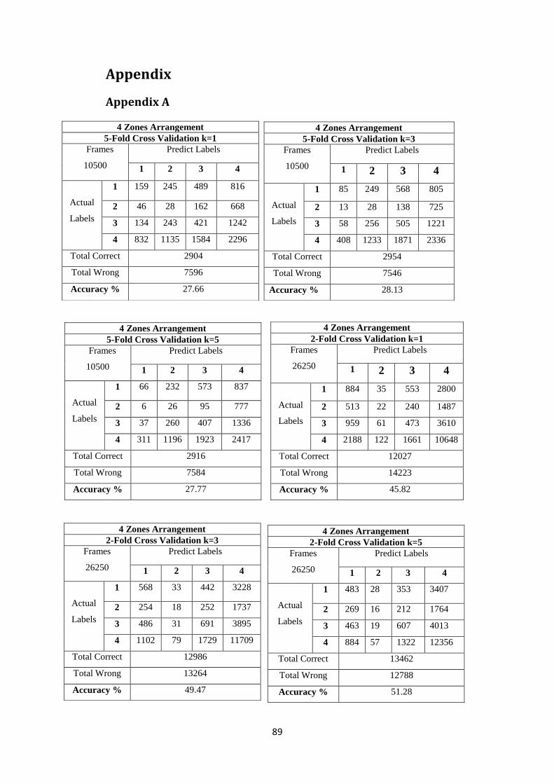
89
Appendix
Appendix A
4 Zones Arrangement
5-Fold Cross Validation k=1
Frames
10500
Predict Labels
1 2 3 4
Actual
Labels
1 159 245 489 816
2 46 28 162 668
3 134 243 421 1242
4 832 1135 1584 2296
Total Correct 2904
Total Wrong 7596
Accuracy % 27.66
4 Zones Arrangement
5-Fold Cross Validation k=3
Frames
10500
Predict Labels
1 2 3 4
Actual
Labels
1 85 249 568 805
2 13 28 138 725
3 58 256 505 1221
4 408 1233 1871 2336
Total Correct 2954
Total Wrong 7546
Accuracy % 28.13
4 Zones Arrangement
5-Fold Cross Validation k=5
Frames
10500
Predict Labels
1 2 3 4
Actual
Labels
1 66 232 573 837
2 6 26 95 777
3 37 260 407 1336
4 311 1196 1923 2417
Total Correct 2916
Total Wrong 7584
Accuracy % 27.77
4 Zones Arrangement
2-Fold Cross Validation k=1
Frames
26250
Predict Labels
1 2 3 4
Actual
Labels
1 884 35 553 2800
2 513 22 240 1487
3 959 61 473 3610
4 2188 122 1661 10648
Total Correct 12027
Total Wrong 14223
Accuracy % 45.82
4 Zones Arrangement
2-Fold Cross Validation k=3
Frames
26250
Predict Labels
1 2 3 4
Actual
Labels
1 568 33 442 3228
2 254 18 252 1737
3 486 31 691 3895
4 1102 79 1729 11709
Total Correct 12986
Total Wrong 13264
Accuracy % 49.47
4 Zones Arrangement
2-Fold Cross Validation k=5
Frames
26250
Predict Labels
1 2 3 4
Actual
Labels
1 483 28 353 3407
2 269 16 212 1764
3 463 19 607 4013
4 884 57 1322 12356
Total Correct 13462
Total Wrong 12788
Accuracy % 51.28

90
Appendix B

91

92