perturbed frequent itemset based classification techniques...
TRANSCRIPT

PERTURBED FREQUENT ITEMSET BASED CLASSIFICATIONTECHNIQUES
Thesis submitted in partial fulfillment
of the requirements for the degree of
MASTERS OF SCIENCE BY RESEARCH
in
COMPUTER SCIENCE
by
RAGHVENDRA MALL
200602018
CENTER FOR DATA ENGINEERING
International Institute of Information Technology
Hyderabad - 500 032, INDIA
JULY 2011

Copyright c© Raghvendra Mall, 2011
All Rights Reserved

International Institute of Information Technology
Hyderabad, India
CERTIFICATE
It is certified that the work contained in this thesis, titled “Perturbed Frequent Itemset Based Classifica-
tion Techniques” by Raghvendra Mall, has been carried out under my supervision and is not submitted
elsewhere for a degree.
Date Adviser: Dr. Vikram Pudi

Dedicated to my indefatigable parents Mr. Narendra Mall andMrs. Anita Mall & my beloved
siblings Dipika and Shivank

Acknowledgments
I would like to take this opportunity to acknowledge and appreciate the effortsof the people who
have helped me during my research and documenting this thesis. I am very grateful to Dr Vikram Pudi,
Dr. Harjinder Singh and Dr P.K. Reddy for providing me with the proper foundations on research which
motivated me to pursue my research in data mining. I sincerely appreciate all theefforts they have
pooled in to provide students like us a learning centre like CDE.
I am very thankful to my peers Pratibha, Lydia, Bhanukiran and Annu for building a congenial en-
vironment for discussion and learning at the lab. I particularly appreciatethe efforts of Pratibha Ma’am
who helped me a lot to improve my technical writing skills. I would like to offer my gratitude to
my friends Aditya, Akshat, Aman, Ankush, Ankita, Arnav, Atif, Himanshu, Ketan, Mohak, Prakhar,
Prashant, Sravanthi, Siddharth, Srijan, Vaibhav and Vinushree for thefruitful discussions and constant
motivation. I am grateful to Prakhar for his contribution in development of PERFICT. I would spe-
cially like to thank Srijan and Neeraj who were always ready for an intellectual discussion and were
extremely patient listeners. As a teaching assistant I would like to thank my juniors, particularly Nahil,
who constantly queried me which helped me revise and kept me updated with state-of-art data mining
concepts.
On a personal front, I would like to thank my family and my dear Sonal who havebeen a great
source of motivation for me in all my endeavors. Finally I would like to thank Godwho has instilled the
resilience and passion in me to pursue my goals wholeheartedly.
v

Abstract
Recent studies in classification have proposed ways of exploiting the association rule mining paradigm.
These studies have performed extensive experiments to show their techniques to be both efficient and
accurate. In this thesis, we propose Perturbed Frequent Itemset based Classification Techniques (PER-
FICT), a novel associative classification approach based on perturbed frequent itemsets. Most of the ex-
isting associative classifiers work well on transactional data where eachrecord contains a set of boolean
items. They are not very effective in general for relational data that typically contains real valued at-
tributes. In PERFICT, we handle real valued attributes by treating items as (attribute,value) pairs, where
the value is not the original one, but is perturbed by a small amount and is a range based value. We
propose a pre-processing step based on perturbation as an alternative to the standard discretization step
to convert real valued attributes into ranges. The PERFICT approaches are built on the Apriori frame-
work for frequent itemsets generation. We also propose our own similarity measure which captures the
nature of real valued attributes and provide effective weights to the frequent itemsets. This MJ similar-
ity measure inherently prunes away the unnecessary frequent itemsets. The probabilistic contributions
of different frequent itemsets is taken into considerations during classification. Some of the applica-
tions where such a technique is useful are in signal classification, medicaldiagnosis and handwriting
recognition. Experiments conducted on the UCI Repository datasets show that variants of PERFICT are
highly competitive in terms of accuracy in comparison with popular associativeclassification methods,
decision trees and rule based classifiers.
We developed PERICASA, PERturbed frequent Itemset based classification for Computational Au-
ditory Scene Analysis(CASA), as an application to HistSimilar PERFICT. It provides a novel architec-
ture for perception of sound waveforms. The purpose of this model is to develop a classifier which can
correctly identify audio waveforms from noisy sound mixtures i.e. to solve theclassical ‘Cocktail Party
Problem’. The architecture is based on Gestalt principles of grouping like Pragnanz, Proximity, Com-
mon Fate and Similarity. The primary idea is that more the ease with which we can identify different
associated feature values, easier it is to identify the sound waveform.
vi

Contents
Chapter Page
1 Introduction . . . . . . . . . . . . . . . . . . . . . . . . . . . . . . . . . . . . . . . . . . 11.1 Notion of Perturbation . . . . . . . . . . . . . . . . . . . . . . . . . . . . . . . . . . 31.2 Problem Definition . . . . . . . . . . . . . . . . . . . . . . . . . . . . . . . . . . . . 41.3 Contributions of Thesis . . . . . . . . . . . . . . . . . . . . . . . . . . . . . . . . .. 51.4 Organization of Thesis . . . . . . . . . . . . . . . . . . . . . . . . . . . . . . . . .. 5
2 Related Work . . . . . . . . . . . . . . . . . . . . . . . . . . . . . . . . . . . . . . . . . 72.1 Classification based on Association Rules . . . . . . . . . . . . . . . . . . . . .. . . 7
2.1.1 Classification based on Association Rules (CBA) . . . . . . . . . . . . . . .. 82.1.2 Classification based on Multiple Association Rules (CMAR) . . . . . . . . . .92.1.3 Classification based on Predictive Association Rules (CPAR) . . . . . .. . . . 102.1.4 Lazy Pruning and Lazy Associative Classifiers . . . . . . . . . . . . . .. . . 11
2.2 Decision Trees . . . . . . . . . . . . . . . . . . . . . . . . . . . . . . . . . . . . . .122.2.1 Information Gain . . . . . . . . . . . . . . . . . . . . . . . . . . . . . . . . . 132.2.2 Avoiding Over-Fitting in Decision Trees . . . . . . . . . . . . . . . . . . . . . 14
2.3 Naive Bayes . . . . . . . . . . . . . . . . . . . . . . . . . . . . . . . . . . . . . . .. 152.4 Discussion . . . . . . . . . . . . . . . . . . . . . . . . . . . . . . . . . . . . . . . . .15
3 PERFICT Algorithm. . . . . . . . . . . . . . . . . . . . . . . . . . . . . . . . . . . . . . 173.1 Issue with discretization . . . . . . . . . . . . . . . . . . . . . . . . . . . . . . . . .173.2 Basic Concepts and Definitions . . . . . . . . . . . . . . . . . . . . . . . . . . . .. . 183.3 The PERFICT Algorithm . . . . . . . . . . . . . . . . . . . . . . . . . . . . . . . . .193.4 Pre-Processing Phase . . . . . . . . . . . . . . . . . . . . . . . . . . . . . . .. . . . 19
3.4.1 Histogram Construction Phase . . . . . . . . . . . . . . . . . . . . . . . . . . 203.5 Transforming the training dataset . . . . . . . . . . . . . . . . . . . . . . . . . .. . . 223.6 Transforming the Test dataset . . . . . . . . . . . . . . . . . . . . . . . . . . .. . . . 233.7 Generating Perturbed Frequent Itemsets . . . . . . . . . . . . . . . . . . . .. . . . . 24
3.7.1 The Join Step . . . . . . . . . . . . . . . . . . . . . . . . . . . . . . . . . . . 273.7.2 The Prune Step . . . . . . . . . . . . . . . . . . . . . . . . . . . . . . . . . . 273.7.3 Record Track Step . . . . . . . . . . . . . . . . . . . . . . . . . . . . . . . . 27
3.8 Naive Probabilistic Estimation . . . . . . . . . . . . . . . . . . . . . . . . . . . . . . 283.9 Time and Space Complexity . . . . . . . . . . . . . . . . . . . . . . . . . . . . . . . 30
vii

viii CONTENTS
4 HistSimilar PERFICT & Randomizedk-Means PERFICT. . . . . . . . . . . . . . . . . . . 324.1 Issues with Hist PERFICT . . . . . . . . . . . . . . . . . . . . . . . . . . . . . . .. 32
4.1.1 Pruning Frequent Itemsets . . . . . . . . . . . . . . . . . . . . . . . . . . . . 324.1.2 Assigning Weights to Itemsets . . . . . . . . . . . . . . . . . . . . . . . . . . 33
4.2 HistSimilar PERFICT . . . . . . . . . . . . . . . . . . . . . . . . . . . . . . . . . . . 334.2.1 MJ Similarity Metric . . . . . . . . . . . . . . . . . . . . . . . . . . . . . . . 334.2.2 Advantages of MJ similarity measure . . . . . . . . . . . . . . . . . . . . . . 36
4.3 Randomizedk-Means PERFICT . . . . . . . . . . . . . . . . . . . . . . . . . . . . . 374.3.1 Disadvantage of Histograms . . . . . . . . . . . . . . . . . . . . . . . . . . . 374.3.2 k-Means approach . . . . . . . . . . . . . . . . . . . . . . . . . . . . . . . . 374.3.3 Advantages ofk-Means . . . . . . . . . . . . . . . . . . . . . . . . . . . . . 38
4.4 Time Complexity . . . . . . . . . . . . . . . . . . . . . . . . . . . . . . . . . . . . . 39
5 PERICASA: An application. . . . . . . . . . . . . . . . . . . . . . . . . . . . . . . . . . 415.1 Introduction . . . . . . . . . . . . . . . . . . . . . . . . . . . . . . . . . . . . . . . .415.2 Traditional Models and Problems faced . . . . . . . . . . . . . . . . . . . . . .. . . 425.3 Gestalt Theory Principles . . . . . . . . . . . . . . . . . . . . . . . . . . . . . . .. . 435.4 The PERICASA Algorithm . . . . . . . . . . . . . . . . . . . . . . . . . . . . . . . .445.5 Dataset Information . . . . . . . . . . . . . . . . . . . . . . . . . . . . . . . . . . .. 455.6 Experimental Results . . . . . . . . . . . . . . . . . . . . . . . . . . . . . . . . . . .455.7 PERICASA Result Analysis . . . . . . . . . . . . . . . . . . . . . . . . . . . . . .. 46
6 Experiments and Results. . . . . . . . . . . . . . . . . . . . . . . . . . . . . . . . . . . . 496.1 Dataset Description . . . . . . . . . . . . . . . . . . . . . . . . . . . . . . . . . . .. 49
6.1.1 UCI datasets . . . . . . . . . . . . . . . . . . . . . . . . . . . . . . . . . . . 496.2 Analysis of PERFICT approaches on Datasets . . . . . . . . . . . . . . . .. . . . . . 50
6.2.1 Analysis of Breast-Cancer Dataset Results . . . . . . . . . . . . . . . . .. . 516.3 Analysis of Diabetes Dataset Results . . . . . . . . . . . . . . . . . . . . . . . .. . . 536.4 Analysis of Ecoli Dataset Results . . . . . . . . . . . . . . . . . . . . . . . . . .. . . 566.5 Analysis of Iris Dataset Results . . . . . . . . . . . . . . . . . . . . . . . . . . .. . . 596.6 Analysis of Image Segmentation Dataset Results . . . . . . . . . . . . . . . . . .. . 616.7 Analysis of Vowel Dataset Results . . . . . . . . . . . . . . . . . . . . . . . . .. . . 636.8 Analysis of Wine Dataset Results . . . . . . . . . . . . . . . . . . . . . . . . . . .. . 666.9 Experimental Evaluation . . . . . . . . . . . . . . . . . . . . . . . . . . . . . . . . .686.10 Execution Times . . . . . . . . . . . . . . . . . . . . . . . . . . . . . . . . . . . . . 71
7 Conclusions . . . . . . . . . . . . . . . . . . . . . . . . . . . . . . . . . . . . . . . . . . 747.1 Contributions . . . . . . . . . . . . . . . . . . . . . . . . . . . . . . . . . . . . . . . 747.2 Future Work . . . . . . . . . . . . . . . . . . . . . . . . . . . . . . . . . . . . . . . .75
Bibliography . . . . . . . . . . . . . . . . . . . . . . . . . . . . . . . . . . . . . . . . . . . . 78

List of Figures
Figure Page
2.1 Associative classification steps . . . . . . . . . . . . . . . . . . . . . . . . . . .. . . 8
3.1 Overlap for the Salary values . . . . . . . . . . . . . . . . . . . . . . . . . . . .. . . 183.2 Hist PERFICT steps . . . . . . . . . . . . . . . . . . . . . . . . . . . . . . . . . . .. 203.3 Equi-Width Histogram . . . . . . . . . . . . . . . . . . . . . . . . . . . . . . . . . . 213.4 Equi-Depth Histogram . . . . . . . . . . . . . . . . . . . . . . . . . . . . . . . . . .213.5 All possible cases of intersecting ranges . . . . . . . . . . . . . . . . . . . .. . . . . 26
4.1 HistSimilar PERFICT steps . . . . . . . . . . . . . . . . . . . . . . . . . . . . . . . . 334.2 Sample Area of Overlap (x axis represents attribute1, y axis represent attribute2) . . . 344.3 Randomizedk-Means PERFICT steps . . . . . . . . . . . . . . . . . . . . . . . . . . 39
5.1 WaveformMJ criteria Results . . . . . . . . . . . . . . . . . . . . . . . . . . . . . . 475.2 Waveformminsupport Results . . . . . . . . . . . . . . . . . . . . . . . . . . . . . 48
6.1 Breast-Cancer MJ criteria results . . . . . . . . . . . . . . . . . . . . . . . . .. . . . 516.2 Result of Bin Size Variations for Breast-Cancer . . . . . . . . . . . . . . .. . . . . . 526.3 Breast-Cancer Minsupport Trends . . . . . . . . . . . . . . . . . . . . . .. . . . . . 536.4 Diabetes MJ criteria results . . . . . . . . . . . . . . . . . . . . . . . . . . . . . . .. 546.5 Result of Bin Size variations for Diabetes . . . . . . . . . . . . . . . . . . . . .. . . 556.6 Diabetes Minsupport Trends . . . . . . . . . . . . . . . . . . . . . . . . . . . .. . . 556.7 Ecoli MJ criteria results . . . . . . . . . . . . . . . . . . . . . . . . . . . . . . . . .. 566.8 Result of Bin Size Variations for Ecoli . . . . . . . . . . . . . . . . . . . . . . .. . . 576.9 Ecoli Minsupport Trends . . . . . . . . . . . . . . . . . . . . . . . . . . . . . .. . . 586.10 Iris MJ criteria results . . . . . . . . . . . . . . . . . . . . . . . . . . . . . . . . .. . 596.11 Result of Bin Size Variations for Iris . . . . . . . . . . . . . . . . . . . . . . .. . . . 606.12 Iris Minsupport Trends . . . . . . . . . . . . . . . . . . . . . . . . . . . . . .. . . . 606.13 Image Segmentation MJ criteria results . . . . . . . . . . . . . . . . . . . . . . . .. 616.14 Result of Bin Size Variations for Image Segmentation . . . . . . . . . . . . . .. . . . 626.15 Image Segmentation Minsupport Trends . . . . . . . . . . . . . . . . . . . . .. . . . 636.16 Vowel MJ criteria results . . . . . . . . . . . . . . . . . . . . . . . . . . . . . . .. . 646.17 Result of Bin Size Variations for Vowel Dataset . . . . . . . . . . . . . . .. . . . . . 656.18 Vowel Minsupport Trends . . . . . . . . . . . . . . . . . . . . . . . . . . . .. . . . . 656.19 Wine MJ criteria results . . . . . . . . . . . . . . . . . . . . . . . . . . . . . . . . .. 666.20 Result of Bin Size Variations for Wine Dataset . . . . . . . . . . . . . . . . .. . . . . 67
ix

x LIST OF FIGURES
6.21 Wine Minsupport Trends . . . . . . . . . . . . . . . . . . . . . . . . . . . . . .. . . 686.22 Time Complexity Comparison . . . . . . . . . . . . . . . . . . . . . . . . . . . . . . 72

List of Tables
Table Page
1.1 Confusion Matrix . . . . . . . . . . . . . . . . . . . . . . . . . . . . . . . . . . . . . 21.2 Classification Quality Evaluation Metrics . . . . . . . . . . . . . . . . . . . . . . . . 3
3.1 Dataset before transformation . . . . . . . . . . . . . . . . . . . . . . . . . . .. . . . 233.2 Dataset after transformation . . . . . . . . . . . . . . . . . . . . . . . . . . . . .. . 233.3 Test dataset before transformation . . . . . . . . . . . . . . . . . . . . . . .. . . . . 233.4 Test dataset after transformation . . . . . . . . . . . . . . . . . . . . . . . . .. . . . 24
5.1 Sample Waveform Dataset . . . . . . . . . . . . . . . . . . . . . . . . . . . . . . .. 445.2 Precision & Execution Times for Waveform . . . . . . . . . . . . . . . . . . . .. . . 46
6.1 Characteristics of the Datasets . . . . . . . . . . . . . . . . . . . . . . . . . . . .. . 506.2 Precision Results . . . . . . . . . . . . . . . . . . . . . . . . . . . . . . . . . . . . .696.3 Execution Time . . . . . . . . . . . . . . . . . . . . . . . . . . . . . . . . . . . . . . 72
xi

Chapter 1
Introduction
Classification has been an age old problem. Early in the4th century BC, Aristotle tried to group
organisms into two classes depending on whether they are beneficial or harmful to a human. He also
introduced the concept of classifying all forms of life for organizing the rich diversity in living organ-
isms. Today classification systems find differentiating features between classes and use them to classify
unknown instances. It has been recognized as an important problem in data mining [33] among other
knowledge discovery tasks.
A classification process involves various stages:
1. Partition Available Data : Theavailable datais the total number of labeled samples of the data
which is available to build a classifier. These samples are bifurcated into two distinct sets, the
training dataand thetest data.
Training Data : It is the set of< transaction, class > pairs (or labeled samples) which are
essential to build the learning model i.e the classification model.
Test Data: It is the set of labeled samples which are part of theavailable dateafter removal of
the training data and are used for evaluation of the predictive model build from the training data.
We generally perform10-fold cross validation for evaluation of classifiers. In10-fold cross vali-
dation, theavailable datais divided into10 equal parts. Each part is consequently selected as the
test dataand the remaining parts are used astraining data. This process of partition ofavailable
data is repeated10 times so that every available sample serves as both a training instance and a
test instance.
2. Classifier Model Construction: The predictive model construction step is the most important
stage of the classification process. Previous studies such as decision trees [7], rule learning [8],
Naive Bayes [18] and statistical methods [1] have developed heuristic/greedy search techniques
for building classifiers. These techniques build a set of rules covering the given dataset and use
1

Actual1 0 Predicted
TP FP 1FN TN 0
Table 1.1Confusion Matrix
them for prediction. The rules encode the relationships between the class variable and other
predictor attributes. Machine learning approaches like SVMs [34] do classification by learning
boundaries between classes and checking on which side of the boundarythe test instance lies.
These learning techniques fall under the category of eager classifiersbecause they build models
in advance and are directly applied on instances from thetesting data. Classifier likekNN belong
to the category of lazy classifiers. They are so called because decision making in their case is
delayed and a model is developed for individual test instances.
Recent studies in classification have proposed ways to exploit the paradigm of association rule
mining for the problem of classification. These methods mine high quality association rules and
use them to build classifiers [4], [8] etc. We refer to these approaches as associative classifiers.
Associative Classifiers have several advantages (1) Frequent itemsets capture all the dominant
relationships between items in a dataset, (2) Efficient itemset mining algorithms exist, (3) These
classifiers naturally handle missing values and outliers as they only deal with statistically sig-
nificant associations, (4) Developed classifiers are robust since onlyfrequent itemsets which are
robust identifiers of a domain are used, and (5) Extensive performance studies [3] have shown
such classifiers to be generally moreaccurate. However, theseassociative classifierssuffer from
the drawbacks of discretization for real valued data. The similarity of individual test instances
with the training data is also lacking. We build a variant of lazy classifier which handle these two
issues efficiently.
3. Evaluation of classification model: There exists a theorem namely the No Free Lunch (NFL)
theorem which states that there can be no classifier which is universally thebest for all datasets.
We evaluate the quality of classification based on certain metrics such as accuracy, precision, re-
call, confusion matrix (Table 1.1) and Area under the ROC Curve (AUC). We provide the formula
to compute some of these metrics in Table 1.2.
Let us consider the simplest classification scenario which is a binary (2 class) problem. The two
classes are positive (1) and negative (0) respectively. Then let the confusion matrix be defined as
2

Name of Measure Formula
Precision TPTP+FP
Recall TPTP+TN
Accuracy TP+TNTP+TN+FP+FN
Table 1.2Classification Quality Evaluation Metrics
shown in Table 1.1.TP here stands for the True Positives or the total number of test instances
correctly predicted by the model as belonging to class1. TN stands for True Negatives which
represents the total correct predictions made by the model that the test instance is negative i.e.
class0. FP stands for False Positives or the total number of negative test instances which were
incorrectly classified as positives.FN stands for False negatives which represents the number of
positive cases that were incorrectly classified as negatives. In our thesis, we focus on the accuracy
quality measure for the evaluation of the classifiers.
1.1 Notion of Perturbation
We introduce the notion of perturbation with an example here. Let us consider a medical diagnostic
dataset consists of features which estimate the plasma glucose concentration, diastolic blood pressure,
2-hours serum insulin, body mass index and diabetes pedigree function incorresponding units along
with the class attribute which refers to the level of diabetes for a patient. Eachof these features take
real values. For example,100-120 plasma glucose concentration range is considered moderate, below
100 is considered low and more than120 is considered high. We have a patient with plasma glucose
concentration as250 units and body mass index be26.5. For each of the other attributes it takes some
real value. There are several such patient records in the dataset. Inassociative classifiers, each value
corresponding to an attribute is called anitem (250 units for plasma glucose concentration is an item).
When we consider a set of items such that each item belongs to a distinct feature, it is called an itemset.
For example, (250 units for plasma glucose concentration,26.5 units for body mass index) is an itemset
of length2. The maximum length of an itemset is equal to the number of features in the dataset apart
from the class attribute. A frequent itemset is an itemset that occurs frequently in the dataset and above
a user defined minimum support threshold.
In the medical diagnostic dataset since we have real values for each predictor attribute, it is difficult
to find exact matches. So one patient may have plasma glucose concentrationof 106.5 units and another
3

patient may have plasma glucose concentration of114.5 units. These two patients have moderate level
plasma glucose concentration but in order to obtain an exact match this similarity cannot be captured.
So discretization of real continuous data is performed. The data is partitionedinto several bins based
on equi-depth histograms or equi-width histograms and partitions (or ranges) are then associated with
consecutive integers. Let us suppose that the number of patients with plasma glucose concentration
between100 units to120 units beN and the standard deviation of all theN (plasma glucose concentra-
tion) measures beσ = 5.5. Thisσ represents the perturbation or the distribution of the plasma glucose
concentration values from the mean value for this partition. So the plasma glucose concentration of
106.5 units will become the range101− 112 units after applying perturbation for the first patient. Sim-
ilarly, the plasma glucose concentration of114.5 units will become the range109 − 120 units for the
second patient. We have a test patient with plasma glucose concentration of115.5 units. Then, we
apply the transformation based on perturbation on the test patient’s attribute value such that his plasma
glucose concentration converts to the range110 − 121 units. So, we see there is a strong overlap of10
units between the test patient and the second patient’s plasma glucose concentration as in comparison
to an overlap of2 units between the test patient and the first patient’s plasma glucose concentration. So
perturbation helps us to capture the inherent similarity between the training dataattribute values and the
test record attribute values. Itemsets which occur frequently and have a strong overlap (greater than a
threshold) are called perturbed frequent itemsets (PFIs).
1.2 Problem Definition
We are provided with a dataset of records, called as thetraining datasetand denoted asD, where
each record is labeled with the class to which it belongs. The problem of classification is defined as:
Problem 1: Given a transactionx to classify (i.e.x is a test record), label it with classci where
ci = argmaxcjp(cj |x) (1.1)
wherep(cj |x) stands for the probability ofcj appearing given thatx has already appeared. In our PER-
FICT approaches, we build model corresponding to eachx. We generate perturbed frequent itemsets
(PFIs), develop techniques to prune them and then estimate the weighted contributionof thesePFIs
for each classcj . The class with the maximum probabilistic contribution is assigned to the given test
recordx.
4

1.3 Contributions of Thesis
We briefly highlight the major contributions of our thesis. We will explore thesepoints in detail at
the conclusion of the thesis.
1. We come up with an effective solution for handling noisy real valued dataand the problem of
exact matches in associative classification by introducing a pre-processing step which converts
the real valued data into range based data using the notion of perturbation.
2. We identify the drawbacks of standard discretization method and avoid it using the perturbation
based pre-processing step. Our pre-processing step helps to obtain the similarity between a train-
ing record’s range and a test record’s range for various attributes.
3. We develop a variation of lazy classifier using Apriori principle to generate perturbed frequent
itemsets corresponding to each test record. Based on the contribution of thePFIs, we proba-
bilistically estimate the class to which each test record belongs.
4. We construct a novelMJ (coined after the originators Mall and Jain) similarity measure which
captures the extent of overlap between a test record’s range and corresponding training record’s
range for the predictor attributes. It helps to efficiently prune and weightthe perturbed frequent
itemsets.
5. We perform an exhaustive analysis of our PERFICT approaches on various datasets and assess
the quality or predictive capability of PERFICT with various state-of-art classifiers.
1.4 Organization of Thesis
The rest of the thesis is organized in the following manner. In Chapter2, we look at theRelated
Work in the field of associative classifiers and rule based classifiers. We shallprovide an exhaustive
coverage of prominent work conducted in these areas in the past decade.
In Chapter3 we look at the PERFICT algorithm and construct the naive Hist PERFICT approach.
In Chapter4 initially we look at the drawbacks of Hist PERFICT. We then come up with a similarity
measure to prune perturbed frequent itemsets and devise a weighting strategy for the contribution of
thePFIs using this measure. It leads to the construction of HistSimilar PERFICT. We thenhighlight
the drawback of histogram based approach and use thek-means clustering method for initial pre-
processing. This leads to the development of Randomizedk-Means PERFICT.
5

In Chapter5 we demonstrate the effectiveness of HistSimilar PERFICT approach by applying it in
the field of auditory scene analysis and come up with PERICASA (PERturbed frequent Itemsets based
Computational Auditory Scene Analysis).
In Chapter6 we provide the evaluation of PERFICT approaches on various diversedatasets and
compare them with various state-of-art classifiers.
In Chapter7 we highlight our conclusions followed by providing some ideas for the future work.
6

Chapter 2
Related Work
Classification is an age-old problem, and several classifiers have been suggested in the last few
decades. Some important classification paradigms include Decision Trees, Naive Bayes, SVM, Statis-
tical and Rule-based classifiers as well as Associative Classifiers. A review of various classification
methods is present in [1]. Since our classifier belongs to the category of Associative Classifiers, we
highlight the differences between various classifiers belonging to this paradigm first. We also reflect
upon other rule-based classifiers like Decision Trees and Naive Bayes.
2.1 Classification based on Association Rules
Classifiers based on Associative Rules involve the following steps:-
• Discover Frequent Itemsets
• Generate Classification Association Rules (CARs).
• Rank and Prune CARs to build a classifier
• Classify a given query test data using the above classifier
The classification process is depicted in Figure 2.1.
In this section, we explain existing classifiers of this paradigm reflecting upon their advantages and
disadvantages.
Association Rules (AR) mining [2] algorithms find all rules in a dataset which satisfy a givensupport
denoted asminsupand a givenconfidencedenoted asminconf thresholds. For example, for the given
7

Figure 2.1Associative classification steps
rule r,a1, a2 → a3 is:-
support(r) = D(a1, a2, a3)
confidence(r) =D(a1, a2, a3)
D(a1, a2)
In the above rule r, the itemseta1, a2 is called theprecedentand the seta3 is called theantecedent.
D(x, y) represents the total occurrence ofx andy together in the datasetD. Classification Association
Rules (CAR) are defined as Association Rules with theantecedentrestricted to only the class attribute.
Hence, for a rule to appear as a CAR in a dataset it should be satisfying thefollowing conditions:
1. supportandconfidenceof the rule should be greater than their respective minimum thresholds.
2. Theantecedentof the rule is always a class variable.
Many efficient algorithms exist today for mining CARs [3, 4] and they generally are modifications to
well-known Association Rule mining algorithms. Since the output of all the CAR mining algorithms
is the same, the first step does not affect the accuracy of the classifier.While analyzing the associative
classifiers we will not delve deep into this step.
2.1.1 Classification based on Association Rules (CBA)
CBA [4] was the first classifier which evolved on the notion of the Association Rule paradigm. For
the first step of finding all the frequent itemsets, it adopts the apriori-like [2] candidate set generation
8

and test approach. For pruning step, to decrease the number of rules generated during the mining step,
it adopts a heuristic pruning method based on a defined rule rank and database coverage.
Definition 1 Rule Rank: Given two rulesri andrj , the rank ofrj is higher than that ofri, (denoted as
ri < rj) if
1. the confidence of the rulerj is higher thanri, or
2. they have the same confidence but the support ofrj is larger than that ofri, or
3. they have same confidence and support values, butrj has fewer items in its precedent i.e. prefer-
ence given to generalized rules
CBA sorts all the CARs according to the above rank definition and selects a small set of high-rank
rules that cover all the tuples in the database as explained in the following procedure:
1. Rules are picked based on their rank, then we traverse through the dataset and find all the tuples
which are correctly classified by the rule.
2. If even a single tuple is not classified correctly by the chosen rule, we discard the rule and go to
step 1. Else we select the rule and remove all the tuples in the dataset that arecorrectly classified
from consideration and return to step 1.
The above procedure is stopped when all the tuples in the dataset are exhausted or when there are no
more rules to consider. The set of rules that are selected are used for building the classifier. A default
rule is added to the set of these rules with theantecedentas the majority class of the dataset and the
precedentas the null set. CBA sorts the selected rules based on their ranks with the default rule having
the lowest rank and uses these rules as the classifier. When a tuple is requested to be classified, it
searches the selected rule set from the highest rank and finds out the first rule that matches the tuple. If
such a rule is found, then its class label is assigned to the new tuple. Note thatevery tuple satisfies the
default rule. Since the default rule classifies to the class with the highest frequency, any tuple that does
not satisfy mined rules is classified to this class.
2.1.2 Classification based on Multiple Association Rules (CMAR)
CMAR [3] acts in a similar fashion as that of CBA, except that it uses multiple rules at the time
of classification to determine the test instance’s class. This is because a single rule at the time of
9

classification may not always robustly predict the correct class. This has been illustrated below:-
a1 =⇒ c1 : support = 0.3, confidence = 0.8
a1, a3 =⇒ c2 : support = 0.7, confidence = 0.7
a2, a4 =⇒ c2 : support = 0.8, confidence = 0.7
To classify a test instancea1, a2, a3, a4, CBA picks the rule with highest confidence that satisfies the
given query, i.e. the first rule and uses it to predict the class asc1. However, a closer look at the rules
suggests that the three rules have similar confidence but the rules predicting classc2 have higher total
confidence. These rules also cover the query much better than the first rule. Hence the decision based
on the last two rules seems to be more reliable. This example clearly indicates thatclassification based
on a single rule could be prone to errors. To make reliable and accurate predictions CMAR proposes
multiple rules contribution for classifying a given test query.
CMAR runs in two phases: (1) Rule generation (2) Classification. A variant of theFP-Growthmethod
[5] for mining association rules is used to mine CARs. The mined CARs are sorted and pruned in a
manner similar as that of CBA. Given a new test instance to classify, CMAR selects the set of rules
satisfying the query from the mined CARs. The chosen rules are divided into groups according to class
labels. All the rules in a group share the same class label and each group has a distinct label. For each
group, the combined effect of all the rules in that group is calculated by a weightedchi-squaredmeasure
given in [6] which was arrived at after extensive experimentation. Formore details of CMAR refer [6].
2.1.3 Classification based on Predictive Association Rules(CPAR)
Associative Classifiers are techniques which have high accuracy but ingeneral they are substantially
slower than the traditional rule-based classifiers like C4.5, FOIL and RIPPER. CPAR tries to combine
the advantages of associative classification and the traditional rule basedclassification.
The rule generation in CPAR is similar to that of FOIL (First-Order InductiveLearning) [7], which
is a greedy algorithm that learns rules to distinguish positive examples from the negative examples. It
repeatedly searches for the current best rule and removes all the positive examples covered by the rule
until all the positive examples in the dataset are covered. The rule miner of CBA, instead of removing
an example after it is covered as in FOIL, maintains a weight for each exampleand decreases it. This
allows covering positive examples multiple times and generating a large set of rules for the classifier.
10

After mining all the rules, each rule is evaluated to determine its prediction power. This is done using
theLaplace expected error estimate[8] which is defined as the follows:
LaplaceAccuracy =nc + 1
ntot + k
where k stands for the number of classes,ntot stands for the total number of examples satisfying the
rule‘s body among whichnc examples belong toc, the predicted class of the rule.
To classify a test instance, CPAR chooses the best ‘k’ rules of each class for prediction using the
following procedure. (1) Select all the rules whose bodies are satisfiedby the example. (2) From the
selected rules, choose the best ‘k’ rules for each class by using theLaplaceAccuracymeasure, and (3)
Compare the average expected accuracy of the best ‘k’ rules of eachclass and select the class with the
highest expected accuracy as the predicted class.
2.1.4 Lazy Pruning and Lazy Associative Classifiers
Some associative classification techniques [9, 10] raise the argument thatpruning classification rules
should be limited to only ‘negative’ rules (those that lead to incorrect classification). In addition, it
is claimed that database coverage pruning often discards some useful knowledge, as the ideal support
threshold is not known in advance. Because of this, these algorithms haveused a late database coverage-
like approach, called lazy pruning, which discards rule that incorrectly classify training objects and
keeps all others.
Lazy pruning occurs after rules have been created and stored, where each training object is taken in
turn and the first rule in the set of ranked rules applicable to the instance is checked. Once all the training
instances have been considered, only the rule that wrongly classified training objects are discarded and
their covered objects are put into a new cycle. The process is repeated until all the training instances
are correctly classified. The results are two levels of rules: the first level contains rules that classified
at least one single training instance correctly and the second level contains rules that were never used
in the training phase. The main difference between lazy pruning and database coverage pruning is that
the second level rules that are held in the memory by lazy pruning are completely removed by database
coverage method. Furthermore, once a rule is applied to the training objects,all objects covered by the
rule are removed (negative and positive) by database coverage method.
Experimental tests reported that methods that employ lazy pruning, such asL3 [9] andL3G [10], im-
prove the classification accuracy than other techniques using database coverage. However, lazy pruning
may lead to very large classifiers, which makes it difficult for a human to comprehend.
11

Unlike the eager associative classifier like CBA, CPAR that extracts ranked CARs from the training
data, the lazy associative classifier [19] induces CARs specific to each test instance. The lazy approach
projects the training data,D, only on those features in the test set,A. From this projected training data
DA, the CARs are induced and ranked, and the best CARs are used. Fromthe set of training instances,
D, only the instances sharing at least one feature with the test instanceA are used to formDA. Then, a
rule setC lA is generated fromDA. SinceDA contains only features inA, all CARs generated fromDA
must matchA. The following steps are involved in building a lazy associative classifier:
Let D be the set of alln training instancesLet T be the set of allm test instancesfor each ti ∈ T dodo
Let Dti be the projection ofD features only fromtiLet Ct
tibe the set of all rulesX → c mined fromDti
sortCtti
according to information gainpick the first ruleX → c ∈ Ct
tiand predict classc
end for
2.2 Decision Trees
Decision trees is a classifier in the form of a flow-chart like tree structure where each node is either:
• a leaf node- reflects the value of the target class attribute of the training instances, or
• a decision node- specifies some test to be carried out on a single attribute-value, with one branch
and sub-tree for each possible outcome of the test.
The steps involved in creating a decision tree classifier include:
1. Tree construction phase
• Initially all the training samples are at the root
• Partition examples recursively based on selected attributes
2. Tree pruning phase
• Identify and remove the branches that reflect noise or outliers
The decision tree construction is a top-down recursive divide-and-conquer procedure. There are two
important notions in decision trees. One is to determine the criteria or heuristic orstatistical measure
12

to select an attribute on the basis of which the training samples are partitioned. Second is to identify
the appropriate stopping criteria to prevent over-fitting or under-fitting. We delve deeper and provide
example of each notion.
2.2.1 Information Gain
Information gain is a statistical measure used for the purpose of attribute selection in C4.5 [7] de-
cision tree classifier. Information gain is usually meant for all categorical attributes but in C4.5 was
extended to continuous-valued attributes by discretizing them. C4.5 approach selects the attribute with
the highest normalized information gain.
Let S be a set consisting of s data samples. Suppose the class attribute hasm distinct values defining
m distinct classes,Ci (for i = 1, ...., m). Letsi be the number of samples of S in classCi. The expected
information needed to classify a given sample is given by
• I(s1, s2, ..., sm) = −pi ×∑
log(pi), wherei = 1 to m, wherepi is the probability that an
arbitrary sample belongs to classCi and is estimated bysi
|S| .
• Let attributeA havev distinct values,a1, a2, ..., av. AttributeA can be used to partitionS into v
subsets,S1, S2, ..., Sv, whereSj contains those samples inS that have valueaj of A.
• If A were selected as the test attribute (i.e., the best attribute for splitting), then these subjects
would correspond to the branches grown from the node containing the set S.
• Let Sij be the number of samples of classCi in a subsetSj . The entropy or expected information
based on the partitioning into subsets by A, is given as
E(A) = (∑ (s1j + ... + smj)
|S|) × I(s1j , s2j , ..smj)
wherej = 1, 2, .., v
• Smaller is the entropy value the greater the purity of the subset partitions.
• For a given subsetSj ,
I(s1j , s2j , ..smj) = −pij ×∑
log(pij)
wherej = 1 to m, andpij =sij
Sj, which is the probability that a sampleSj belongs to classCi.
• The encoding information that would be gained by branching on A is
Gain(A) = I(s1, s2, .., sm) − E(A)
13

• Gain(A) is the expected reduction in entropy caused by knowing the value of attribute A
SplitinfoA(S) = −v
∑
j=1
|Sj |
|S|× log2
|Sj |
|S|
GainRatio(A) =Gain(A)
SplitinfoA(S)
• The attribute which is having the maximum GainRatio() is chosen as the splitting attribute.
2.2.2 Avoiding Over-Fitting in Decision Trees
Generally the decision tree which is generated may overfit the training data and lead to too many
branches. This may reflect anomalies due to noise or outliers and results in poor accuracy for the unseen
samples. RIPPER [11] decision tree classifier emphasizes on this issue.
The RIPPER classifier is built on the principle ofincremental reduced error pruning (IREP ). It handles
noisy data and to prevent over-fitting. The following steps are undertaken for incremental reduced error
pruning:
• The available data is randomly divided into growing set23 and pruning set13 .
• Rules are generated from the growing set or the training data.
• We immediately prune the rules based on a sequence of conditions i.e. delete condition that max-
imizes functionv until no deletion improves the value ofv where v is given by
v(Rule, prunePos, pruneNeg) =p + (N − n)
P + N
whereP (respectivelyN ) is the total number of examples inPrunePos (PruneNeg) andp
(respectivelyn) is the number of examples inPrunePos (PruneNeg) covered byRule.
• This process is repeated until no deletion improves the value of v.
TheIREP approach was extended to multiple classes and RIPPER enhances the classifier further by
rule optimization. The major advantage of RIPPER is that it can handle noisy real world data and
prevent overfitting of the decision tree.
14

2.3 Naive Bayes
Naive Bayes looks at the problem of classification as that of building a conditional probability distri-
butionP (x|ci) accurately over the training data. Once this probabilistic model is available, classification
is done in the following manner:
argmaxciP (ci|x) = argmaxci
P (x|ci × P (ci)
Naive Bayes modelsP (.|ci) by explicitly assuming conditional independence between all items, thus
calculatingP (ci|x) as:
P (x|ci) × P (ci) = P (ci) × Πij ∈ xP (ij |ci) × Πik /∈ x(1 − P (ik|ci))
Such explicit assumptions although are extremely strong. Naive Bayes hascontinued to perform very
well on many datasets. For a detailed information why Naive Bayes performs so well even though it
assumes such strong relationships is illustrated in [12]. The success of Naive Bayes prompted research
into other classifiers which work on similar lines, but having lesser independence assumptions than that
of Naive Bayes. Using ‘if’ and ‘and’ conjunctions we can establish rules out of Naive Bayes classifiers.
2.4 Discussion
After CBA [4] there have been many classification algorithms which tried to usethe associative rule
paradigm for better classification accuracy. Although CBA fared much better than state-of-art classi-
fiers in other paradigms, it still lacked robustness in prediction because ofits single rule classification
mechanism. Later classifiers like CMAR [3] and CPAR [13] took multiple rules intoaccount to make
more reliable predictions. CMAR considers the problem of weighing these groups of rules against each
other in order to classify the test instance.
However, these associative classifiers suffer from certain drawbacks. Though, they provide more rules
and information, redundancy involved in the rules increases the cost in terms of orders of time and com-
putation complexity during the process of classification (database coverage). MCAR [14] determines
a redundant rule by checking whether it covers instances in training setor not. GARC [15] brought
in the notion of compact set to shrink the rule set by converting the rule set toa compact one. Since
the reduction of the redundant rules require a brute force technique, itfails to avoid some meaningless
searching. As we know, the rule generation is based on frequent pattern mining in associative classi-
fication, when the size of data set grows, the time cost for frequent pattern mining increases sharply
which is an inherent limitation of associative classification. A detailed analysis of various associative
15

classifiers is provided by Thabath in [16] and a few recent rule based associative classifiers are provided
in [35],[36],[37].
• A genuine problem with associative classifiers, decision trees and NaiveBayes approach is the
use of discretization of numeric attributes. This situation causes a problem in most of real world
scenarios because records that contain nearly similar values for a realvalued attribute should
support the same rule. Due to discretized matches, the algorithms do not always generate the
required rule.
• There is a also need to reduce the frequent itemsets generated based on their similarity with a
given test instance. Hence, construction of a similarity measure to prune frequent itemsets is also
essential.
Our PERFICT algorithms is a variant of lazy associative classifier and work on these two general
disadvantages of associative classifiers. In PERFICT, we come up with an alternate mechanism for dis-
cretization of real-valued attributes (continuous attributes) and generate frequent itemsets accordingly.
We do not consider the rule generation step rather use the local frequent itemsets and prevent the over-
head of rule searching and database coverage. We also construct a similarity measure to prune frequent
itemsets whose overlap with the test instance is less than a threshold. Being a variant of lazy classifier
typically more work is required to classify all the test instances. However, we come up with a simple
caching mechanism which helps to decrease the work load and space complexity to an extent.
16

Chapter 3
PERFICT Algorithm
In this chapter we introduce the intuition behind usage of perturbation, highlight the basicconcepts
anddefinitionsand develop the naive PERFICT (Hist PERFICT) approach.
3.1 Issue with discretization
Earlier approaches as mentioned in the related work (chapter 2) followed a simple discretization step
for pre-processing. They converted the real valued attributes to ranges. Then these ranges are mapped
to consecutive integers.
Let us suppose “Salary” is an attribute in the training dataset. Let the “Salary” attribute represent the
monthly income of workers in an organization and are specified in the training dataset. Let the incomes
be assigned the range “<= 30, 000”, “ > 30, 000 & <= 65, 000” and “> 65, 000” based on equi-depth
histograms. These ranges are then mapped to consecutive integers1, 2 and3.
There are several issues with discretization. If the bin size is kept small, thenumber of partitions
become high and the ranges obtained would not capture the nature of the dataset effectively. In our
example, if the bin size i.e.(30, 000 or 35, 000) is small then excessive number of ranges would be
generated. Alternatively, if the bin size (30, 000 or 35, 000) is large, two values of the same attribute
positioned at the opposite extremes of the same partition are treated as the equal, though they might
have different contributions. Consider the case, if the income of 2 workers are32, 000 and59, 000.
Then both of them will be mapped to integer2 though their difference is quite large.
The introduction of perturbation allows two different values of the same attribute belonging to the
same partition to be mapped to different ranges. For example, consider a histogram interval30, 000 −
65, 000 say for attributeA1 (i.e. “Salary”) and standard deviation of all the values falling in this his-
togram interval (i.e. the perturbation value,σ) be5, 000. Consider two values belonging to this partition
17

say32, 000 and59, 000. Let the attribute value for one test record be36, 000. A simple discretiza-
tion process will map32, 000, 59, 000 and36, 000 to the interval30, 000 − 65, 000 and replace these
values with an integer2. In other words, both32, 000 and59, 000 are considered to be equally simi-
lar with the test record’s income value (36, 000). But by perturbation1 mechanism, we transform the
“Salary” value of32, 000 to the range27, 000-37, 000 (i.e. 32, 000 ± 5000) and the “Salary” value
of 59, 000 to the range54, 000-64, 000. We see that similarity of32, 000 ± 5, 000 (here perturbation,
σ = 5, 000) is greater than59, 000 ± 5, 000 as its range is closer and intersecting to the test record’s
range (36, 000 ± 5, 000) as depicted in 3.1.
Figure 3.1Overlap for the Salary values
Hence, by introduction of perturbation, we are able to handle this issue with discretization appropri-
ately.
3.2 Basic Concepts and Definitions
Without loss of generality, we assume that our input data is in the form of a relational table whose
attributes are:{A1, A2, A3...An, C}, whereC is the class attribute. We use the termitem to refer to a
attribute-value pair(Ai, ai), whereai is the value of an attributeAi which is not a class attribute. For
brevity, we also simply useai to refer to the item(Ai, ai). Each record in the input relational table
then contains a set of itemsI = {a1, a2, a3...an} wheren represents the total number of attributes. An
itemsetT is defined asT ⊆ I.
A frequent itemset is an itemset whose support (i.e. frequency in the database) is greater than some
user-specified minimum support threshold. We allow for different thresholds depending on the length
of itemsets, to account for the fact that itemsets which have larger length naturally havelow supports.
Let Mink denote the minimum support, wherek is the length of the corresponding itemset.
Use of frequent itemsets for numeric real-world data (i.e. continuous data)is not appropriate as exact
matches for attribute values might not exist. Instead, we use the notion ofperturbation, a term used to
1The notion of perturbation was first introduced inchapter 1
18

convey the disturbance of a value from its mean position. Perturbation represents the noise in the value
of attributes of the items and effectively converts items to ranges. For instance given an itemsetT with
attribute valuesav1, av2 andav3, the perturbed itemset will look like
PFIT = {av1 ± σ1, av2 ± σ2, av3 ± σ3} (3.1)
3.3 The PERFICT Algorithm
The PERFICT algorithm is based on the principle of weighted probabilistic contribution of the Per-
turbed Frequent Itemsets (PFIs). One advantage of this procedure over other associative classifiers is
that there is no rule generating step in PERFICT algorithms. The underlying principle employed in
PERFICT approaches can be stated as
The larger the, extent of similarity of perturbed frequent itemsets with
a given test record’s attribute values, the greater is the similarity
between the given test record and the training records containing those
PFIs
A general outline of the PERFICT algorithm includes the following phases:
• The Pre-Processing phase where three activities are performed:
1. Histogram Construction
2. Transforming the training data based on calculated perturbation
3. Transforming the test data based on calculated perturbation
• The Learning Phase involving apriori like mechanism
• The Classification Phase
Figure 3.2 represents the steps involved in naive Hist PERFICT method. Inthis section, we analyze
each of these phases in detail.
3.4 Pre-Processing Phase
For associative classifiers, it has been widely observed that there is a need of a pre-processing step
where real valued attributes are discretized. In PERFICT, we introducethe concept of perturbation. It
appropriately assigns ranges to these attribute values eliminating the requirement of discretization.
19

Figure 3.2Hist PERFICT steps
3.4.1 Histogram Construction Phase
A histogram is a frequency chart with non-overlapping adjacent intervals calculated upon values of
some variable. It shows what proportion of values fall into each of several partitions. Mathematically, if
n is the total number of observed values, k is the total number of partitions, thehistogrammi must meet
the following condition:
n =k
∑
i=1
mi (3.2)
There are several kind of histograms the equi-width histogram and equi-depth histogram are most pop-
ular.
Equi-Width Histogram
It is the simplest form of a histogram, where all the partitions have same size. The size of each
partition is an important parameter in this kind of histogram.
Equi-Depth Histogram
This histogram is based on the concept of equal frequency or equal number of values in each partition.
The parameter involved is the number of values falling into different sized partitions.
20

Figure 3.3Equi-Width Histogram
Figure 3.4Equi-Depth Histogram
Discussion
For the purpose of classification, equi-depth histograms are more suited because they capture the
intrinsic nature of the random variable or attribute being observed. Moreover, the histogram is not
affected by the presence of outliers. An equi-width histogram on the otherhand is highly affected by
outliers and therefore is a weak choice for the purpose of classification.
For instance, consider:S = {0, 1000, 1002, 1002, 1005, 1005, 1007, 1008, 1011} for a variable. To
divide into 3 partitions of uniform size, the intervals would be0 − 303, 304 − 607 and608 − 1011.
Now the first two partitions are of no significance as0 is an outlier to the set. On the other hand,
equi-depth histogram would divide the interval as0 − 1002, 1005 − 1007, 1008 − 1011 and provide
21

better information for classification purpose. Hence, we prefer equi-depth histograms over equi-width
histograms.
Another histogram which has come into prominence off late is the V-optimal histogram [17]. It is
an example of a more “exotic” histogram. V-optimality is aPartition Rulewhich states that the bucket
boundaries are to be placed as to minimize the cumulative weighted variance of the buckets. The con-
struction of such histograms is a complex process as it is difficult to find the ideal partitions. Moreover,
Any changes to the source parameter could potentially result in having to re-build the histogram en-
tirely, rather than updating the existing histogram. An equi-width histogram does not have this problem.
Equi-depth histograms do experience this issue to some degree, but because the equi-depth construction
is simpler, there is a lower cost to maintain it. To overcome the cost criteria and stillmaintain optimal
buckets, we later on adapt to a much faster clustering algorithmk-Means.
3.5 Transforming the training dataset
The transformation of the training dataset is an integral part of PERFICT approach as observed from
Figure 3.2. Equi-depth histograms are constructed for each attribute with a variable depth value. The
standard deviation of each such partition is computed as well. Let us assume there arek attributes
apart from the class attribute in the training dataset. In order to convert the(attribute, value) pairai to
ai±σi we need a transformation. To obtain these ranges, we use the histogram constructed above. Each
attribute value of a training record is mapped to the corresponding histogrambin using a range query
from the hash table of histograms. The attribute value is transformed to original value± the standard
deviation of all the values in mapped bin. The perturbation is defined as the standard deviation of all the
values of an attribute that are initially hashed into that partition.
We illustrate the procedure with the aid of an example. Letaik represent the value ofith attribute
corresponding tokth record. The histogram bins for theith attribute are represented ashi1, hi2, hi3...hip.
As we are using equi-depth histograms so each partition has equal frequency sayn. Letaik maps tohi3.
hi3 = hash(aik) (3.3)
µhi3=
n∑
j=1
aij
n(3.4)
σi3 =
√
√
√
√
n∑
j=1
(aij − µhi3)2 (3.5)
aik = aik ± σi3 (3.6)
22

whereµhi3represents the mean value for the histogram binhi3 and σi3 represents the standard
deviation of the histogram partitionhi3.
Table 3.1Dataset before transformation
S. No A#1 A#2 A#3 A#4 A#5 A#6 Class
1 v11 v12 v13 v14 v15 v16 C1
2 v21 v22 v23 v24 v25 v26 C2
3 v31 v32 v33 v34 v35 v36 C1
4 v41 v42 v43 v44 v45 v46 C3
5 v51 v52 v53 v54 v55 v56 C2
6 v61 v62 v63 v64 v65 v66 C1
Table 3.2Dataset after transformation
S. No A#1 A#2 A#3 A#4 A#5 A#6 Class
1 v11 ± σ11 v12 ± σ12 v13 ± σ13 v14 ± σ14 v15 ± σ15 v16 ± σ16 C1
2 v21 ± σ21 v22 ± σ22 v23 ± σ23 v24 ± σ24 v25 ± σ25 v26 ± σ26 C2
3 v31 ± σ31 v32 ± σ32 v33 ± σ33 v34 ± σ34 v35 ± σ35 v36 ± σ36 C1
4 v41 ± σ41 v42 ± σ42 v43 ± σ43 v44 ± σ44 v45 ± σ45 v46 ± σ46 C3
5 v51 ± σ51 v52 ± σ52 v53 ± σ53 v54 ± σ54 v55 ± σ55 v56 ± σ56 C2
6 v61 ± σ61 v62 ± σ62 v63 ± σ63 v64 ± σ64 v65 ± σ65 v66 ± σ66 C1
It can be observed from Table 3.2, that each attribute value is replaced by a ranged value. This
process adds perturbation for each attribute value.
3.6 Transforming the Test dataset
The same transformation (as for training dataset) is applied to individual testrecords using training
data histograms.
Table 3.3Test dataset before transformation
S. No A#1 A#2 A#3 A#4 A#5 A#6
1 t11 t12 t13 t14 t15 t162 t21 t22 t23 t24 t25 t263 t31 t32 t33 t34 t35 t36
23

Table 3.4Test dataset after transformation
S. No A#1 A#2 A#3 A#4 A#5 A#6
1 t11 ± σ11 t12 ± σ12 t13 ± σ13 t14 ± σ14 t15 ± σ15 t16 ± σ16
2 t21 ± σ21 t22 ± σ22 t23 ± σ23 t24 ± σ24 t25 ± σ25 t26 ± σ26
3 t31 ± σ31 t32 ± σ32 t33 ± σ33 t34 ± σ34 t35 ± σ35 t36 ± σ36
So, if the test dataset is represented by Table 3.3 before transformation,it becomes Table 3.4 after
transformation.
3.7 Generating Perturbed Frequent Itemsets
To obtain perturbed frequent itemsets (PFIs), we apply the modified Apriori algorithm as described
below:
While developing the algorithm, we assume that the minimum contributing PFIs are perturbed fre-
quent 2-itemsets i.e. frequent itemsets of length2. To obtain these itemsets we identify all attributes in
the training dataset whose value ranges intersect with the test record value ranges.
Let there be k predictor attributes (or feature set) for training dataset along with the class attribute.
The ith attribute is denoted byAi. So the candidate set is a combination of all possible two itemsets
and has the cardinalitykC2. This set can be represented asC2 = {(A1, A2), (A2, A3), ... (Ak−1, Ak)}
whereC2 refers to length2 candidate itemsets.
A candidate itemset is formed if the range of each attribute of the training record intersects with the
corresponding range of the test record. For instance, let the two attributes beA0 andA1. Let the values
of those attributes for thejth training record beaj0 ± σj0 andaj1 ± σj1 respectively. From Figure 3.5,
we can reflect upon all plausible instances, when for both attributeA0 andA1 the ranged based values
of the test record and the training record are intersecting. Hence the count for the candidate itemset
(A0, A1) is incremented by1 and a track of the trainingrecord-id is kept. We make a note that a single
training record may account for multiple candidate itemsets and contributes distinctly in the frequency
of each such candidate itemset.
Once the candidate itemsets have been constructed, we introduce a small prune step based on the
minsupportthreshold which is applied on the count for each candidate itemset. Mathematically, min-
countis defined as:
minsupport100
× size(Currentdataset)
24

Algorithm 1 PERFICT Algorithm
1: Generate candidate 2-itemsets2: while Candidaten-itemsets (n predictor attributes) &&size(Currentdataset) 6= 0 do3: Join Step
Prune StepRecord Track Step
4: for all CandidatesCi,j do5: if count(Ci,j) ≥ minsupport then6: Freq itemset = Freq itemset∪ Ci,j
7: end if8: end for9: end while
Procedure: Generating candidate2-itemsets
1: for all training recordsr do2: for each pair of attributes ai && aj ∈ A do3: if test record’s range(ai) ∩ r’s range(ai) 6= φ &&
test record’s range(aj) ∩ r’s range(aj) 6= φ then4: Candidatei,j = Candidatei,j ∪ r5: end if6: end for7: end for8: for all CandidatesCi,j do9: if count(Ci,j) ≥ minsupport then
10: Freq itemset = Freq itemset ∪ Ci,j
11: end if12: end for
Procedure: The Join Step
1: for all pairsL1, L2 of Freq itemsetk−1 do2: if L1a1
= L2a1andL1a2
=L2a2...
L1ak−2= L2ak−2
and L1ak−1¡ L2ak−1
then3: Ck = a1, a2 ... ak−2, L1ak−1, L2ak−1
4: end if5: end for
Procedure: The Prune Step
1: for all itemsetsc ∈ Ck do2: for each (k-1) subsetss of c do3: if s /∈ Lk−1 then4: deletec from Ck
5: end if6: end for7: end for
25

Procedure: Record Track Step
1: for all itemsetsc ∈ Ck do2: for each k − 1-subsetss of c do3: for each recordr do4: count(r) = 05: end for6: for each recordr contributing in count ofs do7: Increment count(r) by 18: end for9: end for
10: for all recordsr do11: if count(r) = k then12: Keep track of recordr13: end if14: end for15: end for
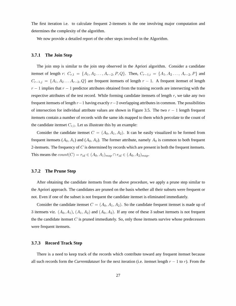
Figure 3.5All possible cases of intersecting ranges
The minsupportis available as user parameter and is directly proportional to degree of pruning that a
user desires. For a very highminsupportvalue very few candidate itemsets will survive. A very low
minsupportvalue tending to0 results in no pruning or elimination of candidate itemsets. As a result
there is a profusion of frequent itemsets. An important aspect of the self-adjustingmincountvalue is
that it prevents over-fitting.
The size of theCurrentdatasetis also variable in our procedure. For 2-itemsets, the value ofCurrent-
datasetis initialized to the size of training dataset. But for generating frequent itemsets of length > 2,
only distinct records which contribute towards the count of at least one perturbed frequent itemset (PFI)
are included inCurrentdataset. A book-keeping strategy for all the record-ids contributing in the fre-
quency of each PFI is followed which is highlighted in the record track step.There are some records
which do not contribute towards any PFI and are removed. Therefore,the value ofCurrentdatasetdoes
not remain same and generally varies.
As the length of itemset increases, for example (A0, A1) → (A0, A1, A2), i.e. from 2 itemsets to 3
itemsets, the size ofCurrentdatasetdecreases. The value ofmincount adjusts accordingly and reduces.
26
The first iteration i.e. to calculate frequent 2-itemsets is the one involving major computation and
determines the complexity of the algorithm.
We now provide a detailed report of the other steps involved in the Algorithm.
3.7.1 The Join Step
The join step is similar to the join step observed in the Apriori algorithm. Consider acandidate
itemset of lengthr: Cr,1 = {A1, A2 . . . , Ar−2, P, Q}. Then,Cr−1,i = {A1, A2 . . . , Ar−2, P} and
Cr−1,j = {A1, A2 . . . Ar−2, Q} are frequent itemsets of lengthr − 1. A frequent itemset of length
r − 1 implies thatr − 1 predictor attributes obtained from the training records are intersecting with the
respective attributes of the test record. While forming candidate itemsets of lengthr, we take any two
frequent itemsets of lengthr−1 having exactlyr−2 overlapping attributes in common. The possibilities
of intersection for individual attribute values are shown in Figure 3.5. Thetwo r − 1 length frequent
itemsets contain a number of records with the same ids mapped to them which percolate to the count of
the candidate itemsetCr,1. Let us illustrate this by an example:
Consider the candidate itemsetC = (A0, A1, A2). It can be easily visualized to be formed from
frequent itemsets (A0, A1) and (A0, A2). The former attribute, namelyA0 is common to both frequent
2-itemsets. The frequency ofC is determined by records which are present in both the frequent itemsets.
This means thecount(C) = rid ∈ (A0, A1)map ∩ rid ∈ (A0, A2)map.
3.7.2 The Prune Step
After obtaining the candidate itemsets from the above procedure, we apply aprune step similar to
the Apriori approach. The candidates are pruned on the basis whetherall their subsets were frequent or
not. Even if one of the subset is not frequent the candidate itemset is eliminated immediately.
Consider the candidate itemsetC = (A0, A1, A2). So the candidate frequent itemset is made up of
3 itemsets viz.(A0, A1), (A1, A2) and(A0, A2). If any one of these3 subset itemsets is not frequent
the the candidate itemsetC is pruned immediately. So, only those itemsets survive whose predecessors
were frequent itemsets.
3.7.3 Record Track Step
There is a need to keep track of the records which contribute toward any frequent itemset because
all such records form theCurrentdatasetfor the next iteration (i.e. itemset lengthr − 1 to r). From the
27

pseudo code it can be observed that for the participation of a record in the count of frequent itemset, the
record must be contributing in the frequency of each of the subsets of thefrequent itemsets.
For example, let us consider a recordr participating for frequent itemset (A0, A1, A2). Thenrid ∈
(A0, A1)map, rid ∈ (A0, A2)map andrid ∈ (A1, A2)map whererid represents record-id and(Ai, Aj)map
represents the map between a frequent itemset and set of all the record ids contributing for that itemset.
3.8 Naive Probabilistic Estimation
Once we have obtained all possible frequent itemsets the final task is the estimation of the class to
which the test record belongs. We devise a formula which comprises two components:
1. For each perturbed frequent itemsetsP (PFIs) of lengthi ≥ 2 we keep track of all the records
contributing tocount(P). These records may belong to different classes. The same itemset may
belong to records pertaining to different classes.
For instance let (A0, A1) be theIth PFI of length2. LetnI be the number of records participating
in the count of this PFI.
nI =∑
j∈C
nIjCj
Cj representsjth class out of the possibleC classes.
So contribution of each PFI oflength ≥ 2 is defined as:
Contri(PFIIi) =∑
I∈Freq(i)
∑
j∈C
nIj
NiCj (3.7)
Ni is the size ofCurrentdatasetfor itemsets of lengthi andPFIIi represents theIth PFI of length
i.
Let us consider the contribution ofPFI13 andPFI24 for a dataset whose size isR. Let us
assumePFI13 occursx1 times for classC1, x2 times for classC2 andx3 for classC3. Similarly,
let PFI24 occury1 times for classC1, y2 times for classC2 andy3 times for classC3. Let R3
andR4 be the reduced size ofCurrentdatasetfor itemsets of length3 and4 respectively.
From the above example, we understand thatPFI13 represents the1st PFI of length3 and
PFI24 represents the2nd PFI of length4. So according to equation (3.7), Contri(PFI13) and
28

Contri(PFI24) can be determined as:
Contri(PFI13) =x1
R3C1 +
x2
R3C2 +
x3
R3C3
Contri(PFI24) =y1
R4C1 +
y2
R4C2 +
y3
R4C3
2. The second part is the heuristics based rank associated with each PFI. We assign higher ranks to
itemsets of larger lengths. However, same weight is associated with the itemsets of similar length.
The allocation resembles ones intuition - Greater the length of the PFI more is the similarity
between training set and test-record and hence a larger contribution towards classification.
Ranki =
∑ip=1 p
∑maxk=2 max − k + 1
(3.8)
where the numerator is sum of all natural numbers from 1 to the lengthi of the frequent itemset
and the denominator is a normalization constant. Heremaxrepresents the maximum number of
attributes in the dataset apart from class attribute as the largest PFI can beof maxlength only. The
formula is similar to that used for assigning weights ink-nearest neighbor classification.
Equation(3.7) is based on same concept as the Laplacian operator mentioned in [8]. A deeper analysis
of the equation(3.7) shows that it converges to1 as the length of PFIs increases. This conforms with
the true nature of the problem as records which are highly similar to a given test record are fewer in
number and play a major role in deciding the class to which the test record may belong.
The overall formula for finding the class conditional probability of a test record becomes
P (C/R) =max∑
i=2
Contri(PFIIi) × Ranki (3.9)
max represents the maximum length itemset possible,P (C/R) contains the contribution from all
classes for a given test record and can also be written as
P (C/R) =aC1
+ aC2+ ...... + aCt
S(3.10)
aCirepresents the contribution of all PFIs for classCi andi varies from1 to t.
This sum of co-efficientsaCican be either greater than or less than1 and is given byS. So to
normalize, each co-efficient is divided byS. This process converts the ratio into a probability mea-
sure. We select that class label as the class for the test record whose co-efficient is maximum i.e
argmaxi{aC1, aC2
, ...aCt}. This naive probabilistic classification technique using the notion of PFIs is
referred as the Hist PERFICT algorithm.
29

The importance of the result lies in the fact that a probabilistic estimation of contribution of all the
classes pertaining to a single test record is available at the end. This can beviewed as an addendum for
detailed analysis and confidence towards classification.
Let us considerP (C/R) = 0.5C1+ 0.3C2
+ 0.2C3. This reveals the contribution of all the PFIs for
a given recordR for each class attribute. Here0.5C1reflects that the PFIs contribute in such a manner
that the probability of the recordR belonging to classC1 is 0.5. Similarly its probability of belonging
to other classes can be determined. We assign the recordR to the classCi which has the maximum
probability corresponding to it.
3.9 Time and Space Complexity
The time complexity of the Hist PERFICT approach is similar to the Apriori algorithmi.e. O(K×N)
whereK is the number of predictor attributes andN is the total number of training records. The space
complexity of Hist PERFICT approach isO(KC2 +K C3). This is because generally the2-itemsets
and3-itemsets are the maximum in number. However, extra effort is required to classify all the test
instances.
We use a simple caching mechanism to decrease this workload to a certain extent. We maintain
a cache pool and it stores a map in the form of< key, data >. Here thekey is aPFI and thedata
contains the id of all the training records contributing to thatPFI and number of records containing that
PFI belonging to each class. Thedata is represented as{< i1, i3, ...ik > , < nC1, nC2
, nC3, ...nCm
>}
wherenCmrepresents the number of records belonging to thatPFI for themth class andik represents
the id of thekth training record. A givenPFI has only one entry in cache and our implementation
stores all the PFIs in main memory. Before generating a newPFI, our approach checks whether a
similar PFI is already in the cache i.e that generatedPFI has a strong overlap>= 1.75 × σi (for each
attributeAi). Otherwise, the PFI is processed and inserted into the cache.
The cache size is limited (2 Mb) for our system and we limit the number of PFIs in the cache to
3, 000. We maintain ids of all the contributing training instances (short int for each id) which help to
determine the records which are active for a particular PFI. Since it is impossible to predict how far in
the future a specificPFI will be used, we choose theLFU (Least Frequently Used) heuristic. It counts
how often aPFI is used and those that are used least are discarded first. We see in the experimental
results that the number of perturbed frequent itemsets generated corresponding to a test instance in a
dataset is not huge and so this cache size is sufficient. This caching mechanism helps to reduce the
computation cost and the space complexity of Hist PERFICT.
30

In the next chapter, we highlight some of the problems with Hist PERFICT andthe way their rectifi-
cation leads to HistSimilar PERFICT and Randomizedk-Means PERFICT method.
31

Chapter 4
HistSimilar PERFICT & Randomized k-Means PERFICT
In this chapter we present two new algorithms which are enhancements to the naive Hist PERFICT
algorithm described in chapter 3. Firstly, we describe the issues with Hist PERFICT. Later we develop
HistSimilar PERFICT and Randomizedk-Means PERFICT followed by time complexity evaluation of
these two approaches.
4.1 Issues with Hist PERFICT
4.1.1 Pruning Frequent Itemsets
Quantitatively, the number of itemsets generated by the Apriori based algorithm are huge and require
a pruning step. However, in the case of Hist PERFICT we generate the set of all possible PFIs without
including an extra pruning step. Some of the itemsets have high contribution in more than one class
which sometimes leads to misclassification. So we need a proper pruning step to make the classifier
more effective.
Let us suppose for a given test recordr, the contribution of aPFII2 = (A0, A1) for P (C/r) beb1C1
andb2C2. TheRank contribution for thePFII2 is same for both the classC1 andC2. Hence it is the
Contri(PFII2) that matters. Supposeb1C1is very close tob2C2
. Let the extent of intersection between
the recordr′s attribute(A0, A1) and the training data records’ attribute(A0, A1) be much greater for
classC1 than classC2. But as theContri(PFII2) is based only on the number of records contributing
to a particular class. So, it does not capture the extent of intersection andresults in misclassification.
32

4.1.2 Assigning Weights to Itemsets
As mentioned earlier, theRank or weight for different length itemsets are different. However,
another major issue with the Hist PERFICT approach is that we assign sameRank or weights to PFIs
of similar length. This has a degrading effect on the accuracy of classifier.
Let us consider for a given recordr, there be 2 PFIs namelyPFII2 andPFIJ2 representing the
Ith andJ th PFI of length2. Let the extent of intersection between the recordr′s attributes andPFII2
be much greater than the extent of intersection between the recordr′s attribute andPFIJ2. So we
should assign weightedRank or rather different weights to PFIs of equal length. Thus, we need to
construct a metric which can capture the range based nature of the PFIs effectively and provide weights
in accordance.
4.2 HistSimilar PERFICT
From Figure 4.1, we observe that an additional step involving a Similarity Calculation is required.
The other steps of the approach are similar and occur in same precedenceas in Hist PERFICT. A simi-
larity criteria is developed during Similarity Calculation step. This similarity measure also contributes
in the Probabilistic Estimation phase and is described below.
Figure 4.1HistSimilar PERFICT steps
4.2.1 MJ Similarity Metric
We define a new similarity measure based on the simple though effective notion of area of overlap.
Let us illustrate by an example. Let us assume for a given test record1st attribute valuea1 = 0.5 and
33

2nd attribute valuea2 = 0.6. Then during the transformation of the test record to perturbed range based
values we mapa1 to a histogram whose standard deviation is0.3 anda2 to a histogram whose standard
deviation is0.4. So the perturbed value for attribute1 and2 becomesa1±σ1 anda2±σ2. Now, let there
be a training recordr for whichr1 = 0.6 andr2 = 0.5. These values also map to the histograms whose
deviations are0.3 and0.4 respectively. Perturbed training record values becomer1 ± σ1 andr2 ± σ2.
σi represents the standard deviation of the histogram to which the record value maps for attributei.
For the attributes1 and2 of the recordr,
AO =(a1 ± σ1) ∩ (r1 ± σ1)
2 × σ1×
(a2 ± σ2) ∩ (r2 ± σ2)
2 × σ2× 22 (4.1)
whereAO represents Area of Overlap and the intersection of the range based values for1st attribute
leads to similarity of0.5 and the intersection of range based values for2nd attribute leads to similar-
ity of 0.7. The similarity values are normalized by taking into account theσ value of the respective
attribute histograms. It can be observed from the formula of area of overlap that only taking into ac-
count the dot products of the similarity for each attribute would lead to a decrease in the overall (since
multiplying one fraction with another fraction). So we introduce an additional multiplicative factor to
obtain the overall area of overlap which has contribution from length of theitemset and is defined as
(itemsetlength)(itemsetlength).
Figure 4.2Sample Area of Overlap (x axis represents attribute1, y axis represent attribute2)
Figure 4.2 represents the example stated above as an illustration. The formulafor Area of Overlap
can be generalized for thejth PFI of lengthk is given by:
AOPFIjk=
k∏
i=1
(ai ± σi) ∩ (ri ± σi)
2 × σi× kk (4.2)
34

ai is theith attribute value for test record andri is theith attribute value for a training recordr andσi is
standard deviation of the histogram partition to which the value maps.
An important constraint imposed on the proposedMJ similarity measure is that PFIs of larger length
must be assigned greater (or worst case equal) weights than PFIs of smaller length. The exponential
(itemsetlength)(itemsetlength) term is introduced to assign larger weights to itemsets of greater length.
An exponential term is chosen because the overlap for an attribute is fractional and can be extremely
small. Thus, a linear multiplicative factor (proportional toitemsetlength) would not be able to provide
the required weight and hence the exponential term is used. However, sometimes if we directly use
the AO based formula, the constrain that PFIs of larger length must be assigned greater weights can
be violated. Without loss of generality, let us consider we have a PFI of length 2 (A1, A2) and from
that PFI another frequent itemset of length3 (A1, A2, A3) is obtained. However, if the intersection for
the 3rd attribute is very small then Area of Overlap is reduced and so similarity of3 length PFI can
be smaller than that of2-length PFI. In order to prevent such an opposing situation we add a term2
×(itemsetlength) to Area of Overlap after taking logarithm (base10) of the Area of Overlap.
MJPFIjk= 2 × k + log10(AOPFIjk
) (4.3)
MJPFIjkrepresents the similarity value for thejth PFI of lengthk with respect to training recordr.
But there are several such records which are contributing in the countof PFIjk with different Area of
Overlaps. So we take average of all such values as the similarity measure for the corresponding PFI.
The attained overlap for each attribute of the PFI is a fraction. The multiplicationof such fractions
to estimate the Area of Overlap can lead to extremely small floating numbers (particularly when the
overlap for an attribute is very small). So, we uselog10() as it allows to map small Areas of Overlap to
feasible floating numbers.
We place the constraint that intersection for each attribute (hereith attribute) must be≥ (0.02× σi).
By maintaining this criteria the similarity value for3-itemset> similarity value for2-itemset.
Proof
Let us consider the worst case example, wherePFI12 andPFI13 represent (A1, A2) & (A1, A2, A3)
respectively (as mentioned above). Let the test record value be(a1 ± σ1, a2 ± σ2, a3 ± σ3) and training
recordr′s value be(r1 ± σ1, r2 ± σ2, r3 ± σ3).
Given the contribution ofA3 or intersection between(a3 ± σ3) ∩ (r3 ± σ3)) in the Area of Overlap
for PFI13 be(0.02×σ3), whereσi is the standard deviation of the histogram to which the record value
35

maps.
MJPFI12 = 2 × 2 + log10(AOPFI12)
= 4 + log10(a1 ± σ1) ∩ (r1 ± σ1)
2 × σ1+ log10
(a2 ± σ2) ∩ (r2 ± σ2)
2 × σ2+ log102
2
= 4 + v + 2 × log102
MJPFI13 = 2 × 3 + log10(AOPFI13)
= 6 + log10(a1 ± σ1) ∩ (r1 ± σ1)
2 × σ1+ log10
(a2 ± σ2) ∩ (r2 ± σ2)
2 × σ2+ log10
(a3 ± σ3) ∩ (r3 ± σ3)
2 × σ3
+log1033
= 6 + v + log10(0.02 × σ3)
2 × σ3+ 3 × log103
= 6 + v + log100.01 + 3 × log103
= 4 + v + 3 × log103
HenceMJPFI12 < MJPFI13 as3 × log103 > 2 × log102 in the worst case situation.
The MJ similarity criteria of intersection≥ (0.02 × σ) is included in Generating Perturbed Frequent
Itemsets step. This criteria is set to determine the Area of Overlap between a test record attributes
and the training record attributes. If this similarity value is below a predeterminedthreshold then the
candidate itemsets are pruned immediately. The Probabilistic Estimation step is modifiedby inclusion
of the MJ criteria. In equation (4.4), we replace theRank term with the MJ similarity measure term to
arrive at the following formula to be used for classification.
P (C/R) =max∑
i=2
Contri(PFIIi) × MJPFIIi(4.4)
This changed probabilistic estimation step is used in HistSimilar PERFICT and Randomizedk-
Means PERFICT algorithms. We throw light at some of benefits obtained by using thisMJ similarity
criteria.
4.2.2 Advantages of MJ similarity measure
1. One of the benefits of using this similarity measure is that we are assigning different weights even
to itemsets of same length based on their area of overlap. More the area of overlap more the
similarity, larger the intersections and greater the weights associated. This is astraight result from
direct proportionality.
Let us consider the two PFIs,PFI1i andPFI2i. The PFIs represent the1st and2nd perturbed fre-
quent itemset of lengthi respectively. Let the Area of Overlap ofPFI1i be greater in comparison
36

to the Area of Overlap ofPFI2i corresponding to a test recordr. Then,MJPFI1i> MJPFI2i
and hence overall weighted contribution ofPFI1i > PFI2i, though the itemsets are of same
length. So, we overcome the earlier problem of sameRank being assigned to all frequent item-
sets of equal length as faced by Hist PERFICT approach.
2. Another unique advantage of this similarity measure is that it intrinsically provides the much
needed pruning step. During the generation of the PFIs, at any stage, ifthe range of intersection
for any attribute of the candidate itemset does not satisfy the MJ criteria then that candidate itemset
is immediately pruned.
The MJ criteria has an inherent requirement that the range of intersectionfor any attribute of the
training record with the corresponding test record’s attribute must be greater0.02 × σi. Hereσi
represents the standard deviation of the histogram bin to which the value mapsfor theith attribute.
This MJ similarity criteria is variable and can be made stricter. It acts as a cut-off threshold and
candidate itemsets not satisfying this threshold are pruned away. So, the requirement of an explicit
pruning step is no longer necessary.
4.3 Randomizedk-Means PERFICT
Before describing the Randomizedk-Means PERFICT approach, we reflect upon some of the prob-
lems faced by histogram based methods.
4.3.1 Disadvantage of Histograms
There are certain limitations to the Histogram based approach for preprocessing the data. The depth
of each histogram for an attribute is kept variable. The histogram construction is a time consuming
process. Further the process of estimation of the best depth for each attribute is manual and cannot
easily be automated (as can be observed in the case of V-optimal histograms). So, same number of
partitions are maintained across each attribute. Sometimes it happens that the variation in the attribute
values is not much and for such an attribute3 or 4 partitions are sufficient but we end up with more
number of bins. This problem can be solved by using a fast clustering technique for preprocessing.
4.3.2 k-Means approach
Thek-Meansalgorithm [18] is a highly popular clustering approach. It can be used very effectively
to identify clusters of data which act as partitions for our method. For our algorithm, we compute the
37

k meansindependently for each attribute and so the data points are all one dimensional. The general
methodology followed comprises of
1. Random selection ofk means for k clusters at the initialization step.
2. Assign data points to clusters based on the minimum distance of the point fromall thek means.
3. Mean value for each of the clusters is re-calculated pertaining to the information obtained from
the points belonging to that cluster.
4. Re-assign data points to the clusters according to the newmean values (based on the earlier
minimum distance criteria).
5. Repeat iteratively till convergence, based on a threshold or unchangedmeans or maximum num-
ber of iterations, has been achieved.
The purpose of this method is to minimize the Squared Sum Error(SSE) i.e distance of each data point
from themean of the cluster to which this point has been assigned.
Once we obtain the clusters along with theirmeans for each attribute, we perform the preprocessing
step. For each training record, we have to apply a transformation to convert the attribute values to
range-based ones. Each value of an attribute is mapped to its nearest cluster mean(for that attribute)
and standard deviation of that cluster is used asσ. Let us say an attributeA1 has a valuea1 which falls
to theith cluster of that attribute and perturbation value for that cluster isσi. Thus the valuea1 of the
training record is now represented asa1 ± σi. This process is also followed for the test data instances.
The steps involved in Randomizedk-Means algorithm is depicted in Figure 4.3. Apart from the use
of k-Means as a preprocessing technique, rest of the phases are same as that forHistSimilar PERFICT
approach.
4.3.3 Advantages ofk-Means
The major contribution of thek-Means method towards our approach is that we calculatek-Means
separately for each attribute and the number of clusters are calculated on the fly. We vary the number of
clusters and identify the best clusters for each attribute based on a threshold:
θ =SSEk−1 − SSEk
k(4.5)
where the numerator represents the difference in the squared sum error for thek-1 clusters andk clusters
and denominator is number of clusters constructed in the process. So whenthe contribution of each
cluster in the squared error is very small i.e. less than a thresholdθ we stop the preprocessing.
38

Figure 4.3Randomizedk-Means PERFICT steps
The approach allows different number of clusters for different attributes and provides a better op-
portunity to capture the inherent similarity within each attribute of a dataset. We now consider the
perturbation as the standard deviation of each cluster. Rest of the procedure is same as that of Hist-
Similar PERFICT algorithm. Thek-Means construction is much faster as in comparison to histogram
construction. Taking advantage of the fact, thek-Means procedure is run multiple times for an accurate
estimation of the clusters as the initialk means were selected randomly. The procedure is henceforth
called Randomizedk-Means PERFICT.
4.4 Time Complexity
The complexity of HistSimilar PERFICT and Randomizedk-Means PERFICT are both much less
than the Hist PERFICT (i.e.O(K × N)) as PFIs are pruned on the basis of MJ similarity measure.
k-Means construction is much faster than equi-depth histogram construction. However, the clusters
produced byk-Means for each attribute are not fixed and capture the values corresponding to an at-
tribute more effectively. In general, the number of PFIs generated by Randomizedk-Means PERFICT
is much more than HistSimilar PERFICT. So the space complexity is smaller for HistSimilarPERFICT
in comparison to Randomizedk-Means PERFICT.
For all thePFIs that can be generated by a test record, the caching mechanism helps to reduce the
space complexity and computation cost. If thePFI is strongly overlapping with a test record attribute
values and is present in the cache, we look at the record ids. So there is no requirement to maintain
a separate entry in the cache for thePFI, thereby reducing the storage space. These are the records
39

which contribute to that cachedPFI and then we calculate the Area of Overlap for these training record
attribute values and the corresponding test record attribute values. This helps to prevent the redundancy
in traversing the entire dataset multiple times for determining the Area of Overlap with the records
belonging to thePFIs of different length which can be generated by the test record.
Let us illustrate this by an example. Suppose we have a dataset of5000 training records and a test
instance which generates150 PFIs which are mapped to the cachedPFIs. If the PFIs were to
be generated from scratch each would traverse all the training recordsand would take750, 000 itera-
tions. Let us suppose that the number of records contributing to eachPFI be200 on an average for a
minsupport of 2%. So the total number of iterations immediately reduces to30, 000 and reduces the
time complexity reduces the time complexity by providing a 25x speed up. This is because the average
number of records corresponding to each PFI in the cache is200 as in comparison to traversing the
entire5000 record dataset for generating a PFI from scratch.
40

Chapter 5
PERICASA: An application
5.1 Introduction
Auditory perception is one of the most important ways of human interaction with the world along
with vision and speech. It is the ‘sound’ which allows us to perform auditory perception. This sound
can be produced by human beings or non-living objects. Moreover, sound acts as a strong stimulus and
forces us as an agent to perform an action. For example, hissing soundof a snake frightens us and voice
of a person we recognize drives us to greet him/her. Auditory perception is performed through the ears,
the organs involved in hearing. Sound waves are pressure waves which propagate in air by compression
and rarefaction. Ear drums convert these sound waves into neural impulses. After conversion they are
represented and analyzed by auditory neurons.
Our primary aim is to come up with a novel computational model for classification of sound wave-
form, articulated in a manner similar to how humans differentiate sounds. We try tosolve the classical
‘Cocktail Party Problem’ i.e. a number of people are talking simultaneously andone is trying to identify
a familiar voice and follow that person’s discussion. Generally, the soundwaves in a party arrive from
multiple sources which intermix to produce a complex waveform. It becomes a difficult task for the
auditory system to separately obtain the one dominant source of interest. The entire process was coined
as ‘Auditory Scene Analysis’ [20, 21, 22] by Bregman in 1990.
The Gestalt group gave the basic principle thatwhole is different from sum of its parts. If a
sound wave is divided into components which act as its features then the original sound wave cannot be
simply sum of these features. They formulated a set of grouping cues which suggested how perceptual
system makes sense of the real world. Some of the principles of perceptual organization are Pragnanz,
Similarity, Good Continuation, Proximity, Common Fate etc.
41

We design an Auditory Scene Analysis model, based on HistSimilar Perturbed Frequent Itemset
Classification Technique, to understand the auditory grouping pressures in humans. We show that the
grouping principles are essential as they provide the ability to classify efficiently.
5.2 Traditional Models and Problems faced
Traditional models developed for CASA follow a top-down architecture putting bits of information
together. They start with the sensory inputs followed by grouping elementary bits into chunks. Then
these chunks are thoroughly investigated by an analysis model. Finally we come up with a working
model of perception. However the use of top down based architecture does not always imply the use of
schema based information. It is the ability to incorporate pressure in all directions within the same level
which is extremely crucial.
A Blackboard Model has been proposed in [23]. In this model the authors motivate their grouping
strategy with the observations that sound can be formed retroactively i.e. asound wave does not have to
be immediately imposed upon its components and a sound is context sensitive. Itis not just the relation-
ship between adjacent components that determines the sound wave - their relationship to surrounding
components is also essential. The above mentioned points are however not mutually exclusive. When
the decision takes a long period then retroactive behavior can be attributedto context sensitive nature.
The model tries to fit to the context efficiently and so the decision is delayed. However the problem with
the approach is that though the intra feature proximity is handled by means of one frequency proximity
expert which works on the entire dataset, the inter feature proximity/similarity is not defined efficiently.
So it is necessary to have a global similarity measure incorporated into the model.
The IPUS architecture [24] was designed to handle complex signal environments from unpredictable
sources and signals whose simultaneous coexistence could distort one another. The model implements
a generic blackboard system for analyzing complex signal situations under the assumption that signal
processing front end is not flexible enough for perception of real world scenarios. There are very few
short comings of the system. However our aim is a different from this system as we want to model the
perception of real world scenarios.
Another model has been proposed in [25] whose aim is segmentation of real world scenarios into a
predefined set of sound elements. This model implements a prediction drivensystem with an abstraction
of auditory events as an internal world model. So the author suggests that only a prediction driven
scheme would be able to work in case of ‘context dependent inferencesin face of interferences.’ A
major concern with this approach is the abstract internal world model which fails to provide a specific
42

representation of attributes/features, inter feature proximity and intra feature similarity essential for
grouping. Another issue is that rather than distinguishing a ‘target’ component from a sound mixture it
provides a prediction of the entire sound scene. The model uses blackboard architecture and maintains
multiple hypotheses at any instant of time. Ear’s Mind [26] is another model which uses the Copycat
model along with a neural network for interpretation of sound waves. TheCopycat architecture has a
probabilistic rule based scheme which is integrated with a neural network forperception of sound. The
problem of rule identification and selection exists in this scheme.
The proposed PERICASA architecture is such that it avoids the shortcomings of the above mentioned
approaches. A fixed partition mechanism is required for modeling auditory perception and so it uses the
concepts of equi-depth histograms for intra feature proximity and novel MJsimilarity measure to find
inter feature similarity. The concept of perturbed frequent itemsets are used for probabilistic estimation
of the identity of the sound waveform followed by a majority choice which helpsin distinguishing and
classifying a ‘target’ from a sound mixture. No rule generation step is required. The above mentioned
qualities are satisfied best by HistSimilar PERFICT. We use the same for the purpose of developing the
model and hence the name PERICASA (PERturbed frequent itemsets basedComputational Auditory
Scene Analysis). Our primary focus is determining or classification of sound and not on feature extrac-
tion. So we build up a computational model for identification of audio waveformsusing a given feature
set.
5.3 Gestalt Theory Principles
The grouping techniques used in PERICASA model are influenced by three principles of Gestalt
group namelyPragnanz, Proximity andCommon Fate. Pragnanz states that the resulting inter-
pretation should always form a good or simple structure.Proximity is the pressure to put together
those elements which are close to one another with respect to other elements.Common fate is the
tendency of the elements to belong together if their behavior is similar. So basedon these three prin-
ciples we come up with a histogram based representation of each feature to capture the intra-feature
proximity. Then a similarity measure named as MJ similarity measure is developed which captures
inter feature similarity in accordance toCommon Fate.
43

5.4 The PERICASA Algorithm
The PERICASA algorithm is built on the HistSimilar PERFICT approach. The basic principle em-
ployed here islarger the extent of overlap of perturbed frequent itemset (PFI) with test sound waveform’s
attribute values greater is the similarity between the test sound waveform and the training instances
containing those PFIs.
A sound or an audio waveform can be expressed usingk features (in the UCI waveform dataset [27]
there are 21 features). We can consider these features as items in a transactional dataset. Then each audio
waveform corresponds to a transaction or record containing thesek features as shown in Table 5.1. We
can use any frequent itemset mining algorithm to mine frequent itemsets from theavailable collection of
audio signals. Larger the extent of overlap of the frequent itemset with a test audio waveform’s attribute
values, greater is the certainity with which we can identify the test sound waveform. For example, if
humans can realizek-1 feature values of a sound waveform and that too frequently then they caneasily
identify that waveform. If a person knows most of the features of a sound waveform then he can identify
that sound even after listening to it very few times. However, human nature isto try to understand a
sound in a probabilistic manner. Compared to when we are able to see a person, we are almost always
uncertain about the source of a sound. For example, even in case of a voice of a familiar person we are
generally confused and sayprobably the voice is of Mr. X. Hence, we use a probabilistic estimation
technique for identification of a sound (audio) waveform. Theminsupport condition also plays a very
Table 5.1Sample Waveform Dataset
S. No A#1 A#2 A#3 A#4 A#5 A#6 Class
1 w11 w12 w13 w14 w15 w16 C1
2 w21 w22 w23 w24 w25 w26 C2
3 w31 w32 w33 w34 w35 w36 C1
4 w41 w42 w43 w44 w45 w46 C3
important role in this model. The minimum support is frequency proximity criterion or in other words
it is minimum experience required for the human being to readily identify one sound waveform. For
example, thisminsupport value is set to 0.1 percent and the training set has5000 instances. Then it
signifies that we are trying to develop a model which can correctly identify anaudio signal after hearing
it just 5 times.
The input format of waveform dataset matches with that of HistSimilar PERFICT and HistSimi-
lar PERFICT well satisfies the constraints of Gestalt Theory Principles. The HistSimilar PERFICT
approach has already been described in detail in chapter4 and is used to develop PERICASA.
44
5.5 Dataset Information
We consider the UCI classification waveform dataset [27]. AC program is available, which can
generate waves pertaining to3 different classes along with noise. Each waveform generates a combi-
nation of2 of 3 base waves. There are21 attributes making up each instance, each attribute value is
normalized to ranges between0 to 6. As we mentioned earlier that it is our assumption that feature
extraction has already been done. So here21 attributes are obtained which include attributes such as
frequency, pitch, loudness, temporal intensities, melfrequency cepstral co-efficients, onsets and offsets
etc. All the attribute values for all instances are coupled with Gaussian noisewith mean0 and variance
1. Uniformity in the database is maintained by generating equal number of records for each class.
5.6 Experimental Results
We conducted experiments over the waveform dataset using the WEKA [28] toolkit. Various classi-
fication techniques such asNeural Networks, SV M , RIPPER, C4.5, PART andNaive Bayes
have been compared to HistSimilar PERFICT. BothNeural Networks andSV M are black box based
approaches. We used a3-layeredNeural Networks and aSMO classifier as aSV M while main-
taining the default parameters in WEKA.C4.5 is a variant of decision tree whereasRIPPER, Naive
Bayes andPART are rule based approaches. We also evaluate the predictive power andexecution time
of our method with associative classifiers likeCBA, CPAR andCMAR usingDM 2 [29] toolkit.
The choice of such learning methods is based on the different strategies they use to generate the rules
and also to compare with black box based mechanisms (Neural Networks andSV M ). The accuracy
and the execution time (in seconds) represent10-fold cross validation results. The configuration of the
system used for running the experiment is a Pentium4 Dual Core Processor with 2 Gb DDR2 RAM.
The code of HistSimilar PERFICT was written inC + +.
Table 5.2 gives an estimate of the predictive power and execution time of various classification tech-
niques for the waveform dataset.Neural Network and SMO take maximum time during model
building phase. We cannot obtain associations in the data using these black box techniques. Decision
tree classifiersC4.5 is fast but low on precision and rule based classifiers likeRIPPER, PART and
Naive Bayes are the fastest but they too compromise with the predictive power. For associative classi-
fiers, large number of frequent itemsets are generated which increasesthe time complexity but provides
quite accurate results and inherent associations are captured. Our PERICASA technique produces the
most accurate result but requires more execution time as the model is built in accordance to each test
45

record. The caching mechanism helps to reduce the execution time. As we traverse the records con-
tributing for eachPFI in the cache, estimating the area of overlap, the execution time is more than other
associative classifiers. It is the inclusion ofMJ similarity measure andminsupport measure which is
primarily responsible for maximizing the accuracy.
Table 5.2Precision & Execution Times for WaveformAlgorithm Accuracy Execution Time
PERICASA 99.56 165.953-layered NN 98.92 1221.35SM0 97.72 378.22RIPPER 76.00 12.8C4.5 75.08 19.8PART 77.42 4.62Naive Bayes 80.00 4.12CBA 78.46 18.7CMAR 83.2 16.43CPAR 80.9 14.28
5.7 PERICASA Result Analysis
The PERICASA model is built on HistSimilar PERFICT which involves several parameters like the
minsupport value, number of partitions or bin size for the histograms and minimum extent of overlap.
The MJ similarity measure works on the criteria that there should be an overlapof (>= 0.02 × σi),
whereσi is the standard deviation of a partition to which test record value maps in theith dimension.
ThisMJ criteria can be varied and expressed mathematically as:
MJj =σj
N
HereMJj represents the minimum extent of overlap condition for thejth dimension andN represents a
natural number. So we can vary the value ofN from {1, 2, ..., 50} as atN = 50 we reach the threshold
condition. The principle concept here is smaller the value ofN , stricter theMJ criteria, greater the
pruning and fewer the number of frequent itemsets generated.
Figure 5.1 represents the effect of the parameterN (i.e. MJ criteria) on the number of frequent
itemsets generated per test record and on the accuracy of the HistSimiliar PERFICT method for various
bin sizes. The bin size represents the percentage of total records in each partition of the histogram and
was varied from14 to 17 (i.e 6 or 7 partitions). As the bin size increases the number of frequent itemsets
per record increases. This is because more training record values hash to each partition and hence more
46

Figure 5.1WaveformMJ criteria Results
values map to a test record’s attribute values. As the value ofN increases theMJ criteria becomes
more stringent and results in pruning. For example, for the bin size17 asN varies from20 to 2, the
number of frequent itemsets reduce from1332 to 73. An important observation was that the bin size
also plays a major role in construction of frequent itemsets. For example, forN = 20, the number of
frequent itemsets generated for the bin size14 is 221 as in comparison to1332 for the bin size17.
Figure 5.1 also provides variations in accuracy with respect to theN (i.e. MJ criteria) for various
bin sizes. The maximum accuracy of99.56 is achieved atN = 1 for bin size14, 15 and17. At small
values ofN (i.e. 1, 2, 3) the results are better for histograms with bin size14 over those with bin size17.
We observe that as the value ofN decreases from20 to 2, the accuracy value increases (in general) with
sharp increase in accuracy at small values ofN . This can be explained logically as for smaller values
of N the unnecessary frequent itemsets are pruned away quickly based on the MJ criteria. The user
specifiedminsupport value was fixed at10.0 for these experiments and it helps to prevent over-fitting.
Figure 5.2 reflects upon the effect ofminsupport on the accuracy and the number of frequent item-
sets generated per test record. As theminsupport value increases the accuracy increases until it reaches
a constant. The value ofN (for MJ criteria) was kept fixed at2 and number of partitions was kept7. As
the value ofminsupport increases from 10% to 12% , the accuracy of classification increases and later
limits to 98.56 and after that it remains constant. However, forN = 1, the accuracy value reaches99.56
for minsupport = 10% and remains the same for higher minsupport values. We know that for the
waveform dataset, the number of frequent itemsets increases as the bin size increases. Butminsupport
value has an antagonistic effect and as it increases more number of candidate itemsets are pruned. This
is because an itemset has to occur more frequently to satisfy theminsupport threshold. We observe that
47

Figure 5.2Waveformminsupport Results
for bin size17, the number of frequent itemsets forminsupport = 10 was73 and forminsupport = 13
was58. Similarly, for the bin size14, the number of frequent itemsets forminsupport = 10 was24
and forminsupport = 13 was18. The maximum length of the frequent itemset was6 and major con-
tributions was of2-itemsets and3-itemsets. This also indicates that the HistSimilar PERFICT approach
does not overfit the training data which has21 attributes.
So, the PERICASA architecture enables the human interaction with sound waveforms and its identi-
fication in an effective manner.
48

Chapter 6
Experiments and Results
In this chapter we look at the experimental results derived on Hist PERFICT, HistSimilar PERFICT
and Randomizedk-Means PERFICT respectively. We first survey the characteristics ofthe dataset used
by us for our experimental setup. Then, we provide an analysis on the influence of various parameters
involved in the PERFICT methodology. We then evaluate the classification effectiveness of the proposed
classifiers with state-of-art classifiers. Finally, we compare the computational cost of the PERFICT
approaches with other classifiers.
6.1 Dataset Description
In this section, we look at the description of the datasets we have considered for these experiments.
The datasets which are used for the experiments are all real life datasets.We pick up12 real attribute
valued datasets from the UCI-ML repository [30]. These 12 datasets from the UCL ML respository
have been selected because these are the most prominent datasets with real valued attributes on which
previous papers have shown their results.
6.1.1 UCI datasets
The datasets considered here are diverse in terms of class distribution, feature space and number
of records. All these datasets share the property of having real valued attributes. We conduct our
experiments on sparse datasets like Diabetes and Wine datasets to dense ones like Vowel Recognition
and Image segmentation datasets. We conduct our experiments on uniformly distributed datasets like
Iris and Waveform datasets to non-uniform datasets like Breast-Cancerand Ecoli datasets. Table 6.1
summarizes the characteristics of the datasets used here.
49

Table 6.1Characteristics of the DatasetsDataset Attributes Classes Records
Breast-Cancer 10 2 699Diabetes 8 2 768Ecoli 7 8 336Heart 13 2 270Glass 10 7 214Iris 4 3 150Pima 8 2 768Segmentation 19 7 2310Vehicle 18 4 846Vowel 10 10 990Waveform 21 3 5000Wine 13 3 178
6.2 Analysis of PERFICT approaches on Datasets
In this section, we reflect upon the effect of various parameters involved in the PERFICT algorithms
on several datasets. We analyze the trends and the variations on accuracy and the number of frequent
itemsets generated based on several parameters like theMJ criteria, histogram size (for Hist PERFICT
and HistSimilar PERFICT) and user-defined minsupport value. This aids in understanding the working
principle of the different PERFICT approaches.
A brief background onMJ criteria was provided in chapter5. We recollect it once more. For both
HistSimilar PERFICT and Randomizedk-Means PERFICT approach, the application of MJ criteria
is one of the most important steps. It is the threshold on the minimum extent of overlap required for
each attribute of the training record with the corresponding test record, otherwise the candidate itemsets
are pruned straightaway. So it provides an effective mechanism to prune the unimportant candidates
(whose contribution is very less) effectively. TheMJ criteria can be varied according to the following
formulation:
MJj =σj
N(6.1)
whereMJj represents the threshold for thejth attribute.σj represents the standard deviation for that
partition to which the training value maps for thejth attribute andN represents a natural number. The
maximum overlap that can occur is equal to2 × σj , when the range based value of the training record
sayr completely overlaps with test record values. AsN is a natural number the MJ criteria is always
smaller than12 of maximum Overlap. We vary theN values from1 to 50 as the minimum overlap
condition is0.02 × σj .
50

The number of histograms or thebin size is also an important parameter for Hist PERFICT and
HistSimilar PERFICT. Thebin size for an attribute represents the percentage of the total values, for the
attribute, that should belong to each histogram in the case of equi-depth histograms. So if thebin size
is given as15, it means the data is divided into7 histograms. Thebin size help to estimate the number
of clustersK for Randomizedk-Means approach. It provides a good approximation except when the
precision value is low we vary the number of clusters too. We see the effectof bin size on the accuracy
and the number of frequent itemsets generated.
Theminsupport value is a user-defined parameter which is an inherent variable in the associative
classifier paradigm. It regulates the number of frequent itemsets produced as it prunes away all the
candidate itemsets below theminsupport threshold and also influences the classification accuracy. It
helps to prevent over-fitting the training data by choice of appropriate threshold values.
6.2.1 Analysis of Breast-Cancer Dataset Results
MJ criteria Results
Figure 6.1Breast-Cancer MJ criteria results
Figure 6.1 reflects upon the effect ofMJ criteria on the accuracy of the HistSimilar PERFICT ap-
proach and Randomizedk-Means approach. Thebin size parameter is used for HistSimilar PERFICT
and is varied from10 to 13. We can observe that for variousbin size values initially the classifica-
tion accuracy remains unaffected. But as the value ofN decreases, theMJ criteria becomes stricter
(minimum extent of overlap condition becomes stricter) and there is an increment in the classification
accuracy for allbin sizes. The best classification accuracy can be achieved for HistSimilar PERFICT
atminsupport = 10% andbin size = 10.
51

When we compare the variations in the accuracy of our proposed classifiers (i.e. HistSimilar and
Randomizedk-Means PERFICT), we observe that optimal classification accuracy is achieved by Ran-
domizedk-Means PERFICT atminsupport = 7% and for7 clusters. As the value ofN increases the
accuracy values decreases linearly and becomes constant for Randomizedk-Means, while for HistSim-
ilar PERFICT it reaches a maximum value of0.966667 and then falls steeply before becoming static
at that value of0.9594. The best overall classification accuracy for breast-cancer dataset is 0.96954 at
N = 2 for Randomizedk-Means PERFICT generating11 frequent itemsets on an average for a given
test record.
Results of Bin Size Variations
The bin size is an important parameter for Hist PERFICT and HistSimilar PERFICT. As we ex-
plained in Chapter 5, thebin size is an estimate of the total percentage of records falling into one
partition. From Figure 6.2, we observe that thebin size is a parameter which plays an important role in
Figure 6.2Result of Bin Size Variations for Breast-Cancer
the classification accuracy and the number of frequent itemsets generatedfor a dataset. We observe an
interesting trend for the accuracy of both Hist and HistSimilar PERFICT as thebin size is varied. The
accuracy curves forms an inverse bell shape i.e. it is high at lowbin size, then decreases and finally
increases to a higherbin size value. A similar trend can be observed in the total number of frequent
itemsets generated for1 fold of a10-fold classification method applied here.
The accuracy value is maximum atbin size = 10% equaling0.95942 and0.96667 for Hist PERFICT
and HistSimilar PERFICT respectively. The total number of frequent itemsetsfor 1 fold which are
contributing for this accuracy are266 and204 respectively. We observe that HistSimilar PERFICT
52

outperforms Hist PERFICT by attaining higher accuracy while generating fewer perturbed frequent
itemsets. The pruning of the candidate itemsets based onMJ criteria is playing a significant role.
Evaluating Minsupport Threshold
Figure 6.3Breast-Cancer Minsupport Trends
From Figure 6.3, we observe that the Breast Cancer dataset attains highaccuracy at higherminsupport
values. We vary theminsupport values from8 to 10 and observe that classification accuracy remains
constant for each PERFICT classifier though the number of frequent itemsets used vary. More frequent
itemsets are generated by Hist PERFICT and Randomizedk-Means PERFICT. The Hist PERFICT ap-
proach does not apply any pruning technique and so larger number of frequent itemsets are generated
whereas theK-Means clustering technique results in partitions which fit the data better. This increases
the total number of frequent itemsets for Randomizedk-Means though it applies theMJ similarity
measure as a pruning criteria. The maximum accuracy of0.96667 is achieved by HistSimilar PERFICT
using just8 frequent itemsets per test record. The maximum length of a frequent itemset is4 and major
contribution is from2-itemsets and3-itemsets. This indicates we prevent overfitting the data though a
variant of lazy classifier.
6.3 Analysis of Diabetes Dataset Results
MJ criteria results
The diabetes dataset is a sparse dataset and provides some interesting results for HistSimilar and
Randomizedk-Means PERFICT approach. From Figure 6.4, we observe that for different bin size
53

Figure 6.4Diabetes MJ criteria results
values the classification accuracy curves follow similar patterns. The curves initially increase to a max-
ima and then follows an undulating pattern. These variations are shown for different bin sizes for the
HistSimilar PERFICT approach. The maximum accuracy is acquired (for HistSimilar PERFICT) for
bin size = 13 atN = 6 generating only34 frequent itemsets for1-fold of 10-fold classification and is
estimated as0.753947.
The Randomizedk-Means PERFICT provides more accurate result at lowerminsupport value (8%
as in comparison to9% for HistSimilar PERFICT). As the value ofN decreases to2 the accuracy
initially increases and achieves maxima twice for Randomizedk-Means PERFICT (atN = 12 andN =
8) while for the HistSimilar PERFICT the accuracy reaches a maximum forN = 6. The Randomized
k-Means PERFICT fits the sparse dataset more suitably and generates167 frequent itemsets for1-
fold. Though the HistSimilar PERFICT generates very few frequent itemsetsbased onMJ criteria, the
classification accuracy remains high.
Varying the Bin Size
Thebin size is an important parameter and is varied from13 to 17 to obtain its influence on accuracy
and number of frequent itemsets for Hist PERFICT and HistSimilar PERFICT.Figure 6.5 indicates that
for the Hist PERFICT approach maximum accuracy of0.735526 is achieved when it generates the
minimum number of frequent itemsets (99) for bin size = 16. This suggests that the frequent itemsets
generated for otherbin sizes are actually contributing negatively for the classification purpose. A stark
difference observed is that the HistSimilar PERFICT generates very few frequent itemsets,34 PF Is
which is nearly3 times lesser than minimum number of frequent itemsets generated by Hist PERFICT
and yet achieves much better prediction accuracy (0.753947). The major reason of decrease is theMJ
54

Figure 6.5Result of Bin Size variations for Diabetes
criteria which prunes away the unnecessary candidate itemsets under strict area of overlap conditions
and is facilitated by the highminsupport value (experiments conducted atminsupport = 9%).
Evaluating Minsupport Threshold
Theminsupport threshold also plays an important role in the number of PF Is generated whichis
reflected in Figure 6.6. We vary theminsupport values from8 to 10 i.e. candidate itemsets which do
Figure 6.6Diabetes Minsupport Trends
not occur in>= 8% of the total data are immediately pruned away. We see that thek-Means captures
the sparsity of training data efficiently. They result in clusters that generate more frequent itemsets
than HistSimilar or Hist PERFICT. From Figure 6.6, we observe that the number of frequent itemsets
decreases linearly for the three methodologies and each has distinct effect on accuracy of the classifier.
55

For Randomizedk-Means PERFICT the accuracy decreases linearly withminsupport value while
it remains constant for HistSimilar PERFICT. This indicates the accuracy hasreached it peak for
Randomizedk-Means PERFICT atminsupport = 8% and the itemsets which are now removed as
minsupport increases are those which contributed positively to the prediction capacity.For HistSimilar
PERFICT, we have achieved optimal accuracy but we can still reduce thenumber of frequent itemsets
asminsupport value increases. However, for HistSimilar PERFICT, the accuracy firstincreases as
minsupport changes to9% from 8% but then decreases and the frequent itemsets generated are de-
creasing linearly. This suggests that initially there were some frequent itemsets which were contributing
negatively atminsupport = 8%, were removed atminusupport = 9% and then important frequent
itemsets started getting pruned. The maximum contributing itemsets are2-itemsets for this dataset.
6.4 Analysis of Ecoli Dataset Results
MJ criteria results
The Ecoli dataset is a non-uniform dataset with records belonging to oneclass in abundance as
in comparison to other classes. We observe the effect ofMJ criteria on such a dataset. Figure 6.7
Figure 6.7Ecoli MJ criteria results
reflects upon the effects ofMJ criteria on the predictive accuracy for differentbin sizes for HistSimilar
PERFICT approach. Higher accuracy values are seen forbin size = 19 andbin size = 20 which
indicates the presence of5 partitions for HistSimilar PERFICT. The maximum accuracy for HistSimilar
PERFICT approach is achieved atN = 4 for bin size = 20 at minsupport = 1% and estimated as
0.818182. The accuracy values varies less for large value ofN but sudden drastic changes occur as the
value ofN decreases. This is because theMJ criteria gets stricter and it can have both positive and
56

negative influence on classification accuracy as it can be observed from Figure 6.7. Forbin size = 18
it has reduced accuracy but forbin size = 20, it increases accuracy tillN reduces to extreme value i.e.
2.
There is a difference of> 4% between the accuracy of Randomizedk-Means PERFICT and HistSim-
ilar PERFICT. This difference can be attributed to fact thatk-Means is able to identify proper clusters
and generates more frequent itemsets than HistSimilar PERFICT. These PFIscontribute in increasing
the predictive power of the classifier. The trend observed is that accuracy is relatively low initially and
reaches an optimum value as the value ofN increases for both HistSimilar PERFICT (0.818182) and
Randomizedk-Means PERFICT (0.866667).
Result of Bin Size Variations
Figure 6.8Result of Bin Size Variations for Ecoli
The bin size is an important parameter for Hist PERFICT and HistSimilar PERFICT approach
and has direct implications on the accuracy of the classifier and the number of frequent itemsets. From
Figure 6.8 we observe that for the HistSimilar PERFICT approach the accuracy increases linearly expect
at bin size = 18 for which the perturbed frequent itemsets generated are maximum i.e.1664 frequent
itemsets per fold. So, this suggests that there is presence of non-essential frequent itemsets atbin
size = 18 whose contribution actually reduces the predictive power of HistSimilar PERFICT. For the
Hist PERFICT approach, the accuracy reaches a peak and then decreases. The maximum accuracy
is attained atbin size = 17 and the number of frequent itemsets generated are1710 per fold. The
maximum classification accuracy of both the classifier is same at0.818182. However, the HistSimilar
PERFICT generates lesser frequent itemsets than Hist PERFICT due to theeffective use ofMJ criteria,
retaining its predictive power.
57

Evaluating Minsupport Threshold
Figure 6.9Ecoli Minsupport Trends
From Figure 6.9, we observe that as theminsupport value increases the accuracy decreases, some-
times becomes constant and then further decreases for the variants of PERFICT approaches. The max-
imum classification accuracy is achieved by Randomizedk-Means PERFICT forminsupport = 1%
and estimated as0.86667. For histogram based Hist PERFICT and HistSimilar PERFICT, the accuracy
is maximum atminsupport = 1% and then decreases to become constant.
The number of frequent itemsets generated per fold also decrease almost linearly asminsupport
value increases. However, thek-Means approach produces more frequent itemsets than Histogram
based approaches as it captures the data more efficiently requiring only3 clusters for attribute3 and
4 and5 clusters for the rest. The best histogram results are also obtained for5 partitions. For Hist
PERFICT, there is a drastic decrease in the number of perturbed frequent itemsets asminsupport value
changes from3% to 4% (from 1306 to 142 frequent itemsets per fold). However, the effect on the
classifier’s accuracy is not so drastic i.e. accuracy decreases from0.7878 to 0.7788. This indicates that
most of the frequent itemsets were not contributing effectively in the predictive ability of Hist PERFICT.
For HistSimilar PERFICT, high classification accuracy is attained with very fewfrequent itemsets. The
role of MJ criteria is extremely important as it prunes away those candidate itemsets which were not
contributing effectively and thus helps HistSimilar PERFICT to provide highly accurate results with less
number of frequent itemsets. On the contrast, Randomizedk-Means PERFICT generate large number
of frequent itemsets (i.e.1609 frequent itemsets atminsupport = 3% as in comparison to142 and118
PFIs of Hist PERFICT and HistSimilar PERFICT for the sameminsupport value) and have the best
predictive power. This indicates that they can efficiently capture the inherent non-uniformity of the data.
58

6.5 Analysis of Iris Dataset Results
MJ criteria results
The Iris dataset is a uniform dataset having equal contribution from the3 classes and linearly inde-
pendent attributes. From Figure 6.10 it can be observed that atN = 2 for all the differentbin sizes
Figure 6.10Iris MJ criteria results
(exceptbin size = 18), the accuracy reaches its peak. In general for different valuesN the accuracy
remains constant. This means that the frequent itemsets generated have higharea of overlap and not
pruned away as theMJ criteria gets stricter. The maximum accuracy for HistSimilar PERFICT occurs
at bin size = 20 or 5 partitions and is estimated to be0.96667.
When we compare the trends between Randomizedk-Means PERFICT and HistSimilar PERFICT,
we observe that asN increases the Randomizedk-Means PERFICT reaches a peak value of0.973333
at N = 4 and then decreases to0.96 before becoming constant. On the other hand, HistSimilar PER-
FICT achieves maximum accuracy of0.96667 at N = 2 before decreasing and becoming constant
at 0.953333. The Randomizedk-Means approach generates the similar number of frequent itemsets
as HistSimilar PERFICT though theminsupport values for evaluation are different i.e.158 frequent
itemsets atminsupport = 4% and155 frequent itemsets atminsupport = 1% respectively.
Result of Bin Size Variations
Thebin size variable plays an important role in Hist PERFICT and HistSimilar PERFICT classifi-
cation accuracy. It also helps to provide an estimate of the best number of partitions that should be used
and helps to provide an approximation for fixing the value ofK in Randomizedk-Means PERFICT
59

Figure 6.11Result of Bin Size Variations for Iris
approach. From Figure 6.11, we observe that as thebin size increases the predictive power increases
for HistSimilar PERFICT and Hist PERFICT though not linearly.
The number of frequent itemsets generated per fold is also increasing as the bin size increases. The
best results are obtained atbin size = 20. For Hist PERFICT, we obtain an accuracy of0.97333 using
165 frequent itemsets for1-fold at minsupport = 1% while for HistSimilar PERFICT the maximum
accuracy attained is0.96667 using155 frequent itemsets for1-fold atminsupport = 1%.
Evaluating Minsupport Threshold
Figure 6.12Iris Minsupport Trends
Figure 6.12 throws light on the effect ofminsupport threshold on accuracy and the number of fre-
quent itemsets generated per fold of classification. As theminsupport value increases the classification
accuracy decreases for Hist PERFICT along with the number of frequent itemsets. The maximum ac-
60

curacy is attained at low values ofminsupport = 1% and then decreases to a minimum of0.94667.
So, the variation in accuracy is not as much as that for Randomizedk-Means PERFICT whose accuracy
varies from0.97333 at minsupport = 4% to 0.91333 at minsupport = 10%. One plausible reason
for this can be the choice ofk-Means for initial clustering.
The number of frequent itemsets per fold generated by Randomizedk-Means is less than Hist PER-
FICT. Though thek-Means fit the data better and generate more frequent itemsets in general but the
presence ofMJ criteria prunes away non-overlapping candidate itemsets. The HistSimilar PERFICT
provide very stable results. The accuracy is maximum atminsupport = 1% and then becomes constant
at0.96 for all minsupport values. However, we see a sharp decline in the number of frequent itemsets
(from 114 to 60) asminsupport changes from3 to 4. The HistSimilar PERFICT approach is the one
which generates the minimum number of frequent itemsets of the three variants with stable predictive
power. The maximum length itemsets are2-itemsets and for some test records even1 or 2 frequent
itemsets was sufficient to predict its class with high precision.
6.6 Analysis of Image Segmentation Dataset Results
MJ criteria results
Figure 6.13Image Segmentation MJ criteria results
The image segmentation dataset is a dense dataset and the evaluation of this dataset is done at high
minsupport values. From Figure 6.13, we detect that for the HistSimilar PERFICT for different values
of bin size, the accuracy is maximum at low values ofN or when theMJ criteria is strict i.e. the extent
of overlap should be quite large. The most accurate results are obtained for bin size = 13 using just11
61

frequent itemsets atminsupport = 12% and estimated as0.761905. As the value ofN increases the
accuracy of the HistSimilar PERFICT decreases in general.
For the Randomizedk-Means PERFICT approach the accuracy increases till a peak is reached at
N = 8 (0.76667) as the value ofN decreases. We observe that for a particular range ofN i.e. from
N = 14 to N = 6, the accuracy of Randomizedk-Means PERFICT was greater than HistSimilar
PERFICT. The higher accuracy can be attributed to the larger number of frequent itemsets generated
by k-Means approach than Histogram based approach (214 frequent itemsets of Randomizedk-Means
PERFICT in comparison to26 frequent itemsets generated by HistSimilar PERFICT).
Results of Bin Size Variations
Figure 6.14Result of Bin Size Variations for Image Segmentation
From Figure 6.14, it can be shown that Hist PERFICT approach is not working effectively for image
segmentation dataset. As thebin size is varied the accuracy of Hist PERFICT decreases drastically
and the number of frequent itemsets generated increase. So a lot of garbage frequent itemsets are being
generated.
On the other hand, the HistSimilar PERFICT approach generates itemsets whichare10 to 20 times
lesser than those generated by Hist PERFICT. TheMJ similarity works efficiently for this dataset
removing the non-essential frequent itemsets and increasing the classification accuracy. As thebin size
increases the accuracy value reaches a maximum atbin size = 13 estimated as0.761905 generating
very few frequent itemsets.
62
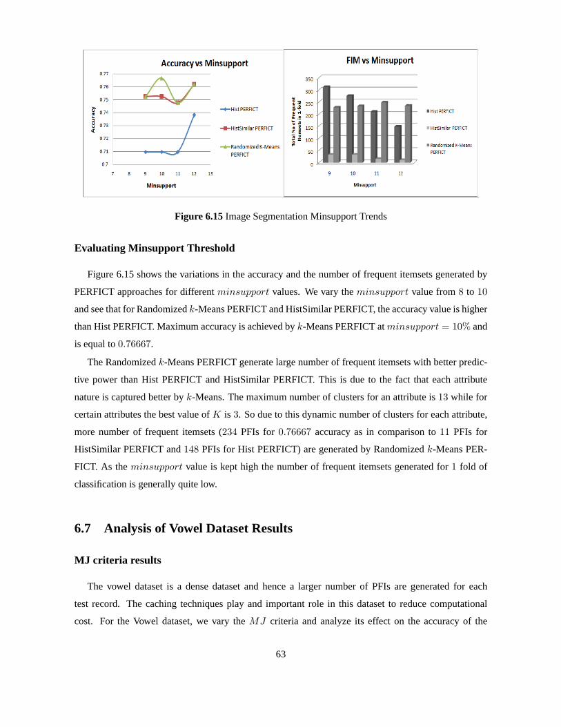
Figure 6.15Image Segmentation Minsupport Trends
Evaluating Minsupport Threshold
Figure 6.15 shows the variations in the accuracy and the number of frequent itemsets generated by
PERFICT approaches for differentminsupport values. We vary theminsupport value from8 to 10
and see that for Randomizedk-Means PERFICT and HistSimilar PERFICT, the accuracy value is higher
than Hist PERFICT. Maximum accuracy is achieved byk-Means PERFICT atminsupport = 10% and
is equal to0.76667.
The Randomizedk-Means PERFICT generate large number of frequent itemsets with better predic-
tive power than Hist PERFICT and HistSimilar PERFICT. This is due to the factthat each attribute
nature is captured better byk-Means. The maximum number of clusters for an attribute is13 while for
certain attributes the best value ofK is 3. So due to this dynamic number of clusters for each attribute,
more number of frequent itemsets (234 PFIs for 0.76667 accuracy as in comparison to11 PFIs for
HistSimilar PERFICT and148 PFIs for Hist PERFICT) are generated by Randomizedk-Means PER-
FICT. As theminsupport value is kept high the number of frequent itemsets generated for1 fold of
classification is generally quite low.
6.7 Analysis of Vowel Dataset Results
MJ criteria results
The vowel dataset is a dense dataset and hence a larger number of PFIs are generated for each
test record. The caching techniques play and important role in this datasetto reduce computational
cost. For the Vowel dataset, we vary theMJ criteria and analyze its effect on the accuracy of the
63
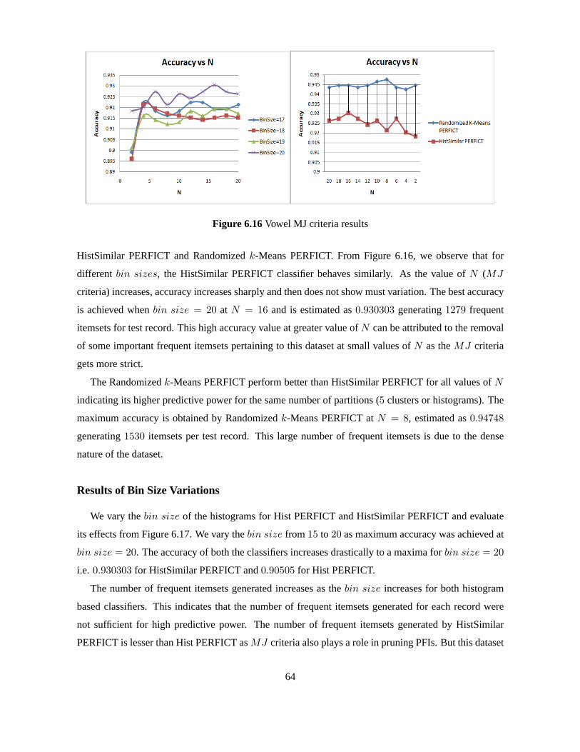
Figure 6.16Vowel MJ criteria results
HistSimilar PERFICT and Randomizedk-Means PERFICT. From Figure 6.16, we observe that for
different bin sizes, the HistSimilar PERFICT classifier behaves similarly. As the value ofN (MJ
criteria) increases, accuracy increases sharply and then does not show must variation. The best accuracy
is achieved whenbin size = 20 at N = 16 and is estimated as0.930303 generating1279 frequent
itemsets for test record. This high accuracy value at greater value ofN can be attributed to the removal
of some important frequent itemsets pertaining to this dataset at small values ofN as theMJ criteria
gets more strict.
The Randomizedk-Means PERFICT perform better than HistSimilar PERFICT for all values ofN
indicating its higher predictive power for the same number of partitions (5 clusters or histograms). The
maximum accuracy is obtained by Randomizedk-Means PERFICT atN = 8, estimated as0.94748
generating1530 itemsets per test record. This large number of frequent itemsets is due to the dense
nature of the dataset.
Results of Bin Size Variations
We vary thebin size of the histograms for Hist PERFICT and HistSimilar PERFICT and evaluate
its effects from Figure 6.17. We vary thebin size from 15 to 20 as maximum accuracy was achieved at
bin size = 20. The accuracy of both the classifiers increases drastically to a maxima forbin size = 20
i.e. 0.930303 for HistSimilar PERFICT and0.90505 for Hist PERFICT.
The number of frequent itemsets generated increases as thebin size increases for both histogram
based classifiers. This indicates that the number of frequent itemsets generated for each record were
not sufficient for high predictive power. The number of frequent itemsets generated by HistSimilar
PERFICT is lesser than Hist PERFICT asMJ criteria also plays a role in pruning PFIs. But this dataset
64

Figure 6.17Result of Bin Size Variations for Vowel Dataset
being dense the pruning is not so effective and the difference in the number of frequent itemsets is quite
small. Hist PERFICT approach generates just28 frequent itemsets more than HistSimilar PERFICT for
the best accuracy atbin size = 20.
Evaluating Minsupport Threshold
Figure 6.18Vowel Minsupport Trends
We vary theminsupport values from1% to5% for the PERFICT approaches as at higherminsupport
values the accuracy was low. The dataset demonstrates the best characteristics for variation of ac-
curacy withminsupport. For all PERFICT methods, the accuracy decreases linearly as the valueof
minsupport increases, the maximum accuracy attained atminsupport = 1%. The best accuracy value
is 0.9474475 was achieved by Randomizedk-Means PERFICT and corresponding accuracy value for
HistSimilar PERFICT and Hist PERFICT are0.930303 and0.90505 respectively.
65
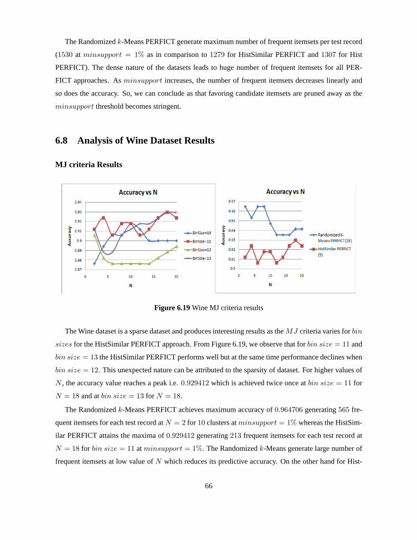
The Randomizedk-Means PERFICT generate maximum number of frequent itemsets per test record
(1530 at minsupport = 1% as in comparison to1279 for HistSimilar PERFICT and1307 for Hist
PERFICT). The dense nature of the datasets leads to huge number of frequent itemsets for all PER-
FICT approaches. Asminsupport increases, the number of frequent itemsets decreases linearly and
so does the accuracy. So, we can conclude as that favoring candidateitemsets are pruned away as the
minsupport threshold becomes stringent.
6.8 Analysis of Wine Dataset Results
MJ criteria Results
Figure 6.19Wine MJ criteria results
The Wine dataset is a sparse dataset and produces interesting results astheMJ criteria varies forbin
sizes for the HistSimilar PERFICT approach. From Figure 6.19, we observe thatfor bin size = 11 and
bin size = 13 the HistSimilar PERFICT performs well but at the same time performance declineswhen
bin size = 12. This unexpected nature can be attributed to the sparsity of dataset. For higher values of
N , the accuracy value reaches a peak i.e.0.929412 which is achieved twice once atbin size = 11 for
N = 18 and atbin size = 13 for N = 18.
The Randomizedk-Means PERFICT achieves maximum accuracy of0.964706 generating565 fre-
quent itemsets for each test record atN = 2 for 10 clusters atminsupport = 1% whereas the HistSim-
ilar PERFICT attains the maxima of0.929412 generating213 frequent itemsets for each test record at
N = 18 for bin size = 11 atminsupport = 1%. The Randomizedk-Means generate large number of
frequent itemsets at low value ofN which reduces its predictive accuracy. On the other hand for Hist-
66

Similar PERFICT, the frequent itemsets which are significantly contributing areremoved at low values
of N or due to tighterMJ criteria resulting in decreasing the predictive power.
Results of Bin Size Variations
Figure 6.20Result of Bin Size Variations for Wine Dataset
We study the effect ofbin size on accuracy and the number of frequent itemsets generated by Hist
PERFICT and HistSimilar PERFICT. The Hist PERFICT approach results are best atminsupport =
5% while best results are obtained for HistSimilar PERFICT atminsupport = 1%. The maximum
accuracy is achieved atbin size = 10 for Hist PERFICT and is equal to0.947059 while maximum
accuracy for HistSimilar PERFICT is attained forbin size = 13.
The number of frequent itemsets generated by Hist PERFICT is much less asin comparison to
HistSimilar PERFICT. This is because theminsupport value is set at5% for Hist PERFICT while it
is just 1% for HistSimilar PERFICT. Maximum number of frequent itemsets (402 per test record) is
generated atbin size = 13 for which the predictive accuracy is greatest for HistSimilar PERFICT. This
indicates that more positively contributing frequent itemsets are generated at bin size = 13.
Evaluating Minsupport Threshold
From Figure 6.21, we observe that as theminsupport value increases, the accuracy decreases for
HistSimilar PERFICT and Randomizedk-Means PERFICT. The number of frequent itemsets generated
by Randomizedk-Means is nearly20 times that generated by HistSimilar PERFICT and Hist PERFICT
at highminsupport values. This indicates that as the dataset is sparse the itemsets whose occurrence
were less but relevant are pruned away at highminsupport values for Randomizedk-Means PERFICT
and HistSimilar PERFICT.
67

Figure 6.21Wine Minsupport Trends
On the other hand, the Hist PERFICT approach works extremely well for this dataset. The nearest
neighbour based ranking technique applied for ranking the frequent itemset contribution has worked
efficiently. As the value ofminsupport increases only the relevant frequent itemsets are left and attain
high predictive power i.e.0.9947059 generating only6 frequent itemsets per record forminsupport =
5%.
6.9 Experimental Evaluation
In this section, we evaluate the PERFICT approaches on 12 real attributeddatasets from the UCI
Machine Learning Repository [30]. We compare PERFICT methods with7 state-of-art classifiers: (1)
widely known and used decision tree classifier C4.5 [7] (its WEKA variant isknown asJ4.8) (2) state-
of-art associative classifiers like CBA [4], CPAR [13] and CMAR [3] (3) rule based classifiers like
RIPPER [11],PART and Naive Bayes.
The pre-processing step of Histogram construction ork-Means construction for the dataset is per-
formed initially and then continuous attribute values are converted to range based values based on per-
turbation. So our techniques prevent the need for a separate discretization step. For the other state-of-art
classifiers, we perform discretization of real valued attributes using an entropy based technique same
as that used inMLC + + library [31]. The associative classifiers like CBA, CPAR and CMAR were
implemented usingDM 2 toolkit [29]. All the other classifiers including C4.5, PART and Naive Bayes
were implemented using theWEKA toolkit. We quantify the classification effectiveness of the classi-
fiers through the conventional accuracy measure (the percentage of test instances correctly classified).
In all the experiments, the accuracy is measured using10-fold cross validation. The configuration of the
68

system used for running the experiments is a Pentium4 Dual Core Processor with2.0 GHz processor
and2 Gb DDR2 RAM. The code of various variants of PERFICT was written inC + +. We provide a
brief analysis of the precision results present in 6.2.
Table 6.2Precision ResultsDataset Hist HistSimilar k-Means CBA CMAR CPAR RIPPER J4.8 PART Naive
PERFICT PERFICT PERFICT Bayes
breast-w 95.94 96.67∗ 96.95 96.28 96.40 95.00 95.10 94.56 93.84 95.99diabetes 73.53 75.39 76.44 73.29 75.80 75.10 74.70 73.66 73.27 75.88ecoli 81.81 81.81 86.67 80.65 81.60 82.01 82.16 84.22 83.63 85.41glass 75.72 79.39 75.71∗ 73.90 70.10 74.40 69.10 66.82 68.22 48.59heart 73.33 77.04 81.11 81.47 82.20 82.60 80.70 77.57 79.86 83.49segmentation 73.81 76.19 77.14∗ 61.44 63.23 65.63 - 86.60 87.08 69.04iris 97.33 96.66∗ 97.33 96.47 94.00 94.70 94.00 96.00 94.00 96.00pima 73.55 76.18∗ 76.71 72.51 75.10 73.80 73.10 73.83 75.26 74.30vehicle 61.67 65.24 75.23 68.70 68.80 69.50 68.60 72.45 71.51 44.79vowel 90.51 93.03∗ 94.74 72.03 76.78 75.46 - 71.22 70.02 63.63waveform 95.26 99.56 99.56 78.46 83.20 80.90 76.00 75.08 77.42 80.00wine 95.29 95.29 96.47∗ 94.96 95.00 95.50 91.60 93.82 93.25 96.62
Comparison with Associative Classifiers
We first compare our techniques with associative classifiers like CBA, CMAR and CPAR. These
associative classifiers perform discretization based on entropy and are not using any similarity measure
(like MJ similarity criteria) for pruning unimportant candidate frequent itemsets. Theygenerate, rank
and apply rules to classify test records. In our experiments, the parameters for all the classifiers were
set to standard values as reported in literature. For CBA, CMAR and CPAR, theminsupport threshold
was set equivalent to that used for PERFICT approaches and theconfidence is set to50% with pruning
enabled.
Associative classifiers like CBA, CPAR and CMAR perform well in case ofsmall and sparse datasets
like Breast Cancer, Heart, Ecoli, Wine etc. The general trend is that CPAR is better than CMAR which
outperforms CBA. However, when it comes to dense datasets like Waveform, Vowel and Image Segmen-
tation datasets, these classifiers fail to make an impact. One reason might be generation of too many
rules with similar confidence belonging to different classes. Another reason is pruning away of rules
due to highminsupport values used for dense datasets. This increases the chance of no CAR matching
a test instance.
When compared to the PERFICT approaches, the associative classifiersare unable to outperform
Randomizedk-Means PERFICT for any dataset. The HistSimilar PERFICT has a win-loss-tie estimate
69

of 8-4-0 and Hist PERFICT has a win-loss-tie estimate of 6-6-0 with CPAR. Some datasets like wave-
form and vowel dataset deserve special mention. The PERFICT methodologies are able to increase the
accuracy by15%-20% over classifiers like CBA, CMAR and CPAR. We investigated the reason for
such dramatic improvement and observed that the role of perturbation for transforming the data value to
range based values and theMJ similarity criteria play a drastic role. Classifiers like CBA and CMAR
generate large number of100% confident rules (homogeneous partitions), so that breaking ties and se-
lecting the rules to apply becomes hard and erroneous. The number of frequent itemsets generated for
the PERFICT approach for dense datasets like waveform and vowel are quite high (> 1000 per test
record) at lowminsupport values. But due toMJ similarity criteria, only those candidate itemsets
survive whose area of overlap with given test record attribute values issignificant.
Comparison with Decision Trees and Rule Based Classifiers
The Randomizedk-Means PERFICT overpowers C4.5 (J4.8) decision tree classifier for 11 datasets
out of 12 real attributed datasets and the win-loss-tie estimates for HistSimilar PERFICT and Hist PER-
FICT with C4.5 are 8-4-0 and 6-6-0 respectively. The C4.5 algorithm outperforms the PERFICT ap-
proaches for Image Segmentation dataset. The decision tree classifier is able to form a well balanced
tree for the segmentation dataset which helps to increase its accuracy drastically. Moreover, the number
of frequent itemsets generated per fold by the PERFICT approaches is quite less for a dense dataset like
Image segmentation. This scarcity of frequent itemsets adversely affects the predictive power of the
PERFICT approaches as in comparison to other classifiers.
Rule based classifiers like RIPPER, PART and Naive Bayes were straightforwardly outperformed
by Randomizedk-Means PERFICT for9 UCI datasets. For RIPPER classifier, we were unable to
acquire the results for Image Segmentation and Vowel dataset. RIPPER hada win-loss-tie estimate of
0-10-0 with Randomizedk-Means PERFICT and 3-7-0 with HistSimilar PERFICT and 4-6-0 with Hist
PERFICT. However, rule based classifiers like PART and Naive Bayesare most accurate classifiers for
Image segmentation and Heart dataset respectively. They are able to capture the inherent nature of the
dataset by generation of simple rules. The win-loss-tie estimate for PART classifier to Randomized
k-Means PERFICT is 1-11-0, to HistSimilar PERFICT is 4-8-0 and to Hist PERFICT is 5-7-0. The
RIPPER and PART classifiers do not drastic variations with other state-of-art classifiers for the various
datasets. But for certain datasets like Glass and Vehicle, the accuracy ofthe Naive Bayes algorithm is
below par. It is the inherent assumption of independence between attributes which leads to its downfall
here. The win-loss-tie estimate for Naive Bayes classifier to Randomizedk-Means PERFICT is 2-10-0,
to HistSimilar PERFICT is 4-8-0 and to Hist PERFICT is 6-6-0.
70

Analyzing PERFICT
The Randomizedk-Means PERFICT algorithm outperforms other algorithms over 8 datasets and
is among top3 for 11 datasets. The performance ofk-Means PERFICT over other algorithms is ex-
ceptional for Waveform, Vowel, Vehicle and Ecoli datasets. The inclusionof MJ similarity measure is
primarily responsible for high precision results. It helps to prune away theitemsets which are not essen-
tial for classification and gives the appropriate weight to eachPFI necessary for classification. Another
reason for high success rate of Randomizedk-Means is that it captures the noisy nature of attributes of
different datasets. Superiority of Randomizedk-Means over HistSimilar and Hist PERFICT approach
is due to the fact that variable number of points can belong to a cluster as opposed to equi-depth his-
togram. This is because the size of a cluster is not fixed while frequency ofeach bin has to be same for
equi-depth histogram.
The necessity for having a variable for the number of clusters or bins canbe seen by the fact that
in Diabetes dataset where the number of clusters or bins for each attribute isbest set to8 while for the
Ecoli dataset the number is5 as there is little variation in value of each feature. The PERFICT methods
work well at highminsupport values for dense datasets. For datasets like Glass, Image and Wine, the
Randomizedk-Means PERFICT is among the top3 classifiers. Hence, it is suitable for tasks like Image
recognition and Handwriting recognition too.
6.10 Execution Times
Table 6.3 highlights the execution time obtained for various classifiers. Our cache size is set to 3000
frequent itemsets. All time correspond to the total time spent (in seconds) using 10-fold cross validation.
For small datasets like Iris, Wine, Heart, Glass and Ecoli, the PERFICT algorithms perform much better
than associative classifiers like CBA, CMAR and CPAR. Their execution time iscomparable to decision
tree classifier like C4.5 but rule based classifiers like RIPPER, PART and Naive Bayes require least
computation time. These results are reflected in Figure 6.22. Associative classifiers generate frequent
itemsets and then select rules based on rank, order and coverage. Rulegeneration and rule selection
is a time consuming process and so the computation cost increases. However, rule based classifiers
are simpler by nature and generate few rules to perform classification. The PERFICT methodology
implements extra work, namely frequent itemset generation for each test instance, it usually generates
fewer distinct perturbed frequent itemsets for smaller datasets and so execution time is low.
For large datasets like Vehicle, Vowel and Waveform, the PERFICT algorithms are worst performer
with execution times being5 to10 times greater than other state-of-art classifiers. Two factors contribute
71

Table 6.3Execution TimeDataset Hist HistSimilar k-Means CBA CMAR CPAR RIPPER J4.8 PART Naive
PERFICT PERFICT PERFICT Bayes
breast-w 5.32 6.33 5.75 3.6 3.52 2.2 1.1 1.6 0.62 0.4diabetes 5.04 4.52 5.33 2.68 2.60 1.12 0.8 0.9 0.2 0.12ecoli 2.25 1.52 2.68 5.21 4.32 3.27 1.92 4.62 0.76 0.52glass 2.18 1.18 1.26 2.35 2.12 2.01 0.8 1.8 0.48 0.22heart 3.66 3.32 7.76 8.92 7.18 4.77 3.8 4.1 2.38 2.15segmentation 3.80 1.75 2.45 4.65 4.42 4.20 - 3.68 2.24 1.8iris 1.29 0.24 0.29 5.4 5.62 4.52 1.8 5.5 0.23 0.12pima 6.02 6.12 5.66 6.67 6.56 4.88 2.2 5.4 1.26 1.02vehicle 28.25 40.5 40 19.2 19.6 13.5 8.6 16.8 6.43 4.56vowel 33.33 32.2 26.66 17.8 18.2 14.3 - 15.2 7.68 5.2waveform 182.2 165.95 172.55 39.6 38.2 26.5 12.8 19.8 8.4 5.65wine 2.31 2.25 3.15 12.8 11.6 8.2 4.5 9.2 2.25 1.8
for this, one is the size of the dataset. This is an inherent problem with associative classifiers i.e.
as the size of the dataset increases or the number of attributes increases,the time complexity increases.
Another major reason is the extra work, namely the generation of frequentitemsets for each test instance.
For large datasets, greater number of distinct perturbed frequent itemsets are generated which fill in the
cache. So, removal of frequent itemsets based on least frequently used (LFU) principle is performed
multiple times and it increases the time complexity.
Figure 6.22Time Complexity Comparison
72

Other classification techniques too become computationally expensive for datasets (like Vowel, Wave-
form etc.) with greater number of attributes or datasets with more number of records. However, simple
classification technique like Naive Bayes classifiers have the lowest computational cost.
73

Chapter 7
Conclusions
In this thesis, we studied in detail the problem of numeric data classification where training records
are represented by numeric real valued variables. We force the issue that using perturbation for trans-
formation of real attribute values to ranges can provide an appropriate alternative to discretization.
Our main focus here has been on classification based on perturbed frequent itemsets. Frequent
itemsets are a nice way to capture statistical relationships between the class variable and the remaining
variables because they lead to robust identifiers of the problem domain andcan handle missing values
and outliers. The major issue studied in this thesis is to avoid the discretization stepfor noisy real valued
data, mine all perturbed frequent itemsets based on modified Apriori principle, use a new similarity
measure for weighting and pruning perturbed frequent itemsets to combine their contribution to form a
robust probabilistic classifier.
7.1 Contributions
The main contributions in this work are as the follows:
1. We introduce the notion of perturbation to map noisy real valued data into ranges. Initially, we
perform a pre-processing step i.e. Histogram construction for Hist andHistSimilar PERFICT
andk-Means based clustering for Randomizedk-Means PERFICT. We then use each histogram
partition or cluster and calculate its standard deviation. This standard deviation orσ is then used
to convert each data value, mapped to that partition or cluster, into ranges.
2. We highlight the drawbacks of discretization step used by most of the standard associative clas-
sifiers (like CBA, CMAR etc.) and avoid it by using a pre-processing step.The pre-processing
step uses perturbation to convert real attribute values into ranges and helps to capture the inherent
similarity between a training record’s range and a test record’s range.
74

3. We construct Hist PERFICT methodology using the Histogram construction and a modified Apri-
ori principle to generate perturbed frequent itemsets. Using a self-adjusting mincount, we prune
candidate itemsets and prevent over-fitting. Based on the Laplacian contribution and Ranks of the
perturbed frequent itemsets, we probabilistically estimates the contribution of eachPFI towards
a class variable.
4. We highlight the problems faced by Hist PERFICT namely generation of large number of fre-
quent itemsets and allocation of equal weights to frequent itemsets of same length with varying
overlaps. This lead to the construction of a new similarity measure,MJ similarity criteria, which
required the candidate itemsets to have a minimum extent of overlap in each dimension with the
test record’s attribute values. Based on their extent of overlap, the candidate frequent itemsets are
pruned (if overlap is less than minimum) and weighted. Thus, frequent itemsets of same length
can have different contributions in the final probabilistic estimate.
5. We introducedk-Means as a clustering technique to cluster the data more efficiently. Thek-Means
construction is faster than Histogram construction, so the process can berepeated several times
as the initialk means are chosen at random. The Randomizedk-Means PERFICT generates
more frequent itemsets than HistSimilar PERFICT and was adapted to use theMJ similarity
criteria. Our experimental results show that PERFICT approaches are generally more accurate
than existing state of the art classifiers like CBA, CMAR, C4.5, Naive Bayes, PART etc.
6. The PERFICT approaches are a variant of lazy classifier, a model isbuilt specific to each test
instance. In order to maintain the space and time complexity, we use a caching strategy which
helps to reduce the computational cost to a great extent for certain datasets. Smaller the number
of distinct frequent itemsets generated for each test record, lower would be the execution time.
However, for large scale datasets, the computational cost and space requirement can be improved
to some extent.
7.2 Future Work
The work presented in this thesis can be extended and improved in certain aspects. Possible direc-
tions are given below:
1. To improve the efficiency of modified Apriori candidate generation step described inchapter3, a
frequent pattern growth (FP-growth [32]) method can be utilized. The FP-growth method builds a
75

highly dense FP-tree for the training data set, where each training object isrepresented by at most
one path in the tree. As a result, the length of each path is equal to the number of the frequent
items in the transaction representing that path. This type of representation is very useful for the
following reasons. (a) All of the frequent itemsets in each record of the original database are
given by the FP-tree, and because there is much sharing between frequent items, the FP-tree is
smaller in size than the original database. (b) The FP-tree construction requires only two database
scans, where in the first scan, frequent itemsets along with their supportin each transaction are
produced, and in the second scan, the FP-tree is constructed. Thus our Apriori based method can
be extended to FP-growth method and can save computation space and time.
2. Sometimes it is observed that datasets for image,signal processing and handwriting recognition
have a very large feature space or suffer from the curse of dimensionality. So in order to reduce
the computation cost (K × N ) i.e. K predictor attributes, we can perform a data pre-processing
technique like Principal Component Analysis (PCA) or Linear Discriminant Analysis (LDA). We
might have to compromise slightly with the accuracy but this reduction in the numberof attributes
will make PERFICT approaches quite scalable.
3. We need to come up with a more efficient caching technique (caching technique shown inchapters
3 and4). Rather than tracking the individual contributing record-ids for each frequent itemset,
we need to devise a mechanism which keeps track of the number of recordsbelonging to each
class. We also need to obtain a rough estimate of the overlap in each dimension corresponding to
that frequent itemset. By just maintaining a count of the records belonging toeach class and an
average estimate of overlap in each dimension for all those records, the space complexity can be
reduced and the cache size can be increased from3, 000 to 10, 000 frequent itemsets. However,
averaging the extent of overlap in each dimension will have an impact on accuracy.
4. The PERFICT are more suitable to small scale datasets from which frequent meaningful patterns
can be extracted. However, temporal datasets like time varying speech dataset where the attribute
values evolve with time are not suitable for the approach as the mapped ranges and similarity
would evolve with time.
76

Related Publications
• Raghvendra Mall, Prakhar Jain and Vikram Pudi, “PERFICT: Perturbed Frequent Itemset Based
Classification Technique” accepted at22nd International Conference on Toolkits in AI, ICTAI
2010, Arras, France.
• Raghvendra Mall, Prakhar Jain, Vikram Pudi and Bipin Indurkiya, “PERICASA” accepted at9th
IEEE International Conference on Cognitive Informatics, IEEE ICCI 2010, Beijing, China.
77

Bibliography
[1] T.S. Lim, W.Y. Loh and Y.S. Shih. A comparision of prediction accuracy, complexity and traininig time of
thirty-three old and new classification algorithms. Machine Learning, 40(3), 203-228, 2000.
[2] R. Agarwal and R. Srikant. Fast algorithms for mininig association rules, In Very Large Databases VLDB,
1994.
[3] W. Li, J. Han and J. Pei. CMAR: Accurate and efficient classification based on multiple class-association
rules, In ICDM, 2001.
[4] B. Liu, W. Hsu and Y. Ma. Integrating classification and association rule mining. In Proceedings of 4th
International Conference on Knowledge Discovery of Data (KDD), August, 1998.
[5] J. Han, J. Pei and Y. Yin. Mining frequent patterns without candidate generation. In Proceedings of 29nd
ACM SIGMOD Intl. Conference on Management of Data, May, 2000.
[6] Wenmim Li Classification based on multiple association rules. Master’s Thesis, Simon Fraser University,
2001.
[7] J. R. Quinlan. C4.5: Programs for Machine Learning. Morgan Kaufmann, 1993.
[8] P. Clark and R. Boswell. Rule induction with CN2: Some recent improvements. In the proceedings of 5th
European Session on Learning, 151-163, 1991.
[9] E. Baralis and P. Torino. A lazy pruning to classificationrules. In the proceedings of International Conference
on Data Mining, Maebashi, Japan, 2002.
[10] E. Baralis, S. Chiusano and P. Graza. On support thresholds in associative classification. In the proceedings
of ACM Symposium on Applied Computing, Nicosia, Cyprus, ACMPress, 553-558, 2004.
[11] W. Cohen. Fast Effective Rule Induction. In the proceedings of the Twelfth International Conference on
Machine Learning, 115-123, 1995.
[12] P. Domingos and M.J. Pazzani. Beyond Independence: Conditions for the optimality of simple bayesian
classifier. In Proceedings of International Conference on Machine Learning, 1996.
[13] X. Yin and J. Han. CPAR: Classification based on Predictive Association Rules. In SDM, 2003.
[14] T. Fadi, C. Peter and Y. Peng. : MCAR: Multi-class classification based on association rule. IEEE Interna-
tional Conference on Computer Sytems and Applications, 127-133, 2005.
[15] G. Chen et al A new approach to classification based on association rule mining. Decision Suport Systems,
42, 674-689, 2006.
78

[16] F. A. Thabtah. A review of associative classification mining. Knowledge Engineering Review, 22, (1),
37-65, 2007.
[17] V. Poosala, P. Haas, Y. Ioannidis and E. Shekita Improved Histograms for Selectivity Estimation of Range
Predicates. Proceedings of the ACM SIGMOD, ACM Press, 1996,294-305.
[18] R. Duda and P. Hart. Pattern Classification and scene analysis. John Wiley and Sons, New York, 1973.
[19] A. Veloso, W. Meira and M. Zaki Lazy Associative Classifier. Sixth International Conference on Data
Mining, 2006.
[20] A. Bregman and P. Ahad Demonstrations of Auditory SceneAnalysis: The Perceptual Organization of
Sound. MIT Press, 1996.
[21] C. Plack Auditory Perception. Psychology Press Limited, 2004.
[22] G. Brown Auditory Scene Analysis. Computer Speech and Hearing, COM4210/COM6450.
[23] D. Godsmark and G. Brown Context-Sensitive Selection of Auditory Organizations: A Blackboard Model.
Computational Auditory Scene Analysis, 1998, 139-155.
[24] F. Klassner and N. V. Lesser The IPUS Blackboard Architecture as a Framework for CASA. In Proceedings
IJCAI workshop on CASA, 1995.
[25] D. Ellis Prediction Driven Computational Auditory Scene Analysis for Dense Sound Mixtures. ESCA
workshop on the Auditory Basis of Speech Perception, Keele UK, July, 1996.
[26] R. Dor Ear’s Mind , a computer model of the fundamental mechanism of the perception of sound. Master
Thesis.
[27] http : //mlearn.ics.uci.edu/databases/waveform/
[28] http : //www.cs.waikato.ac.nz/ml/weka
[29] http : //www.comp.nus.edu.sg/ dm2/
[30] http : //mlearn.ics.uci.edu/databases/
[31] R.Kohavi, D. Sommerfield and J. Dougherty Data Mining using MLC++: A machine learning library in
C++. In Tools with Artificial Intelligence, pages 234-245, 1996.
[32] J.Han, J. Pei and Y.Yin Mining frequent itemsets without candidate generation. In Proceedings of the 2000
ACM SIGMOD International Conference on Management of Data,Dallas, Texas, TX: ACM Press, pp.
1-12, 2000.
[33] U.M. Fayyad, G.P. Shapiro, P. Smyth and R. Uthurusamy Advances in Knowledge Discovery and Data
Mining. AAAI/MIT Press, 1996.
[34] N.Cristianini and J.S.Taylor An Introduction to Support Vector Machines. Cambridge University Press,
2000.
[35] Jie Dong and Jie Lian BitTableAC: Associative classification algorithm based on BitTable 2010 International
Conference on Intelligent Control and Information Processing (ICICIP), pp. 529-532, 2010.
79

[36] Pie-Yi Hao and Yu-De Chen A novel associative classification algorithm: A combination of LAC and
CMAR with new measure of weighted effect of each rule group 2011 International Conference on Machine
Learning and Cybernetics (ICMLC), pp. 891-896, 2011.
[37] ACN: An Associative Classifier with Negative Rules 11thIEEE International Conference on Computational
Science and Engineering pp. 369-375, 2008.
80