frequent itemsets association rules evaluation · – generate high confidence rules from each...
TRANSCRIPT

Frequent Itemsets
Association Rules Evaluation


� Itemset
� A collection of one or more items
▪ Example: {Milk, Bread, Diaper}
� k-itemset
▪ An itemset that contains k items
� Support (σσσσ)
� Count: Frequency of occurrence of an itemset
� E.g. σ({Milk, Bread,Diaper}) = 2
� Fraction: Fraction of transactions that contain an itemset
� E.g. s({Milk, Bread, Diaper}) = 40%
� Frequent Itemset
� An itemset whose support is greater than or equal to a minsup threshold, � � �
minsup
� Problem Definition
� Input: A set of transactions T, over a set of items I, minsup value
� Output: All itemsets with items in I having � � � minsup
TID Items
1 Bread, Milk
2 Bread, Diaper, Beer, Eggs
3 Milk, Diaper, Beer, Coke
4 Bread, Milk, Diaper, Beer
5 Bread, Milk, Diaper, Coke

null
AB AC AD AE BC BD BE CD CE DE
A B C D E
ABC ABD ABE ACD ACE ADE BCD BCE BDE CDE
ABCD ABCE ABDE ACDE BCDE
ABCDE
Given d items, there are
2d possible itemsets
Too expensive to test all!

The Apriori Principle
• Apriori principle (Main observation):
– If an itemset is frequent, then all of its subsets must also be frequent
– If an itemset is not frequent, then all of its supersets cannot be frequent
– The support of an itemset never exceeds the support of its subsets
– This is known as the anti-monotone property of support
)()()(:, YsXsYXYX ≥⇒⊆∀

Found to be frequent
Frequent
subsets

Found to be
Infrequent
Pruned
Infrequent supersets
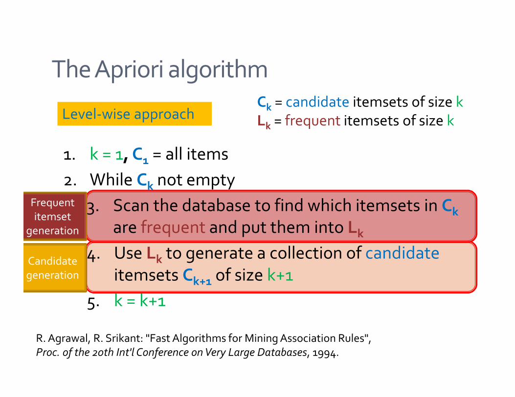
R. Agrawal, R. Srikant: "Fast Algorithms for Mining Association Rules",
Proc. of the 20th Int'l Conference on Very Large Databases, 1994.
The Apriori algorithm
Level-wise approachCk = candidate itemsets of size k
Lk = frequent itemsets of size k
Candidate
generation
Frequent
itemset
generation
1. k = 1, C1 = all items
2. While Ck not empty
3. Scan the database to find which itemsets in Ck
are frequent and put them into Lk
4. Use Lk to generate a collection of candidate
itemsets Ck+1 of size k+1
5. k = k+1

� Basic principle (Apriori):
� An itemset of size k+1 is candidate to be frequent
only if all of its subsets of size k are known to be
frequent
� Main idea:
� Construct a candidate of size k+1 by combining
two frequent itemsets of size k
� Prune the generated k+1-itemsets that do not
have all k-subsets to be frequent

� Given the set of candidate itemsets Ck, we need to compute
the support and find the frequent itemsets Lk.
� Scan the data, and use a hash structure to keep a counter for
each candidate itemset that appears in the data
TID Items
1 Bread, Milk
2 Bread, Diaper, Beer, Eggs
3 Milk, Diaper, Beer, Coke
4 Bread, Milk, Diaper, Beer
5 Bread, Milk, Diaper, Coke
TransactionsCk

� Create a dictionary (hash table) that stores
the candidate itemsets as keys, and the
number of appearances as the value.
� Initialize with zero
� Increment the counter for each itemset that
you see in the data

Suppose you have 15 candidate itemsets
of length 3:
{1 4 5}, {1 2 4}, {4 5 7}, {1 2 5}, {4 5 8},
{1 5 9}, {1 3 6}, {2 3 4}, {5 6 7}, {3 4 5},
{3 5 6}, {3 5 7}, {6 8 9}, {3 6 7}, {3 6 8}
Hash table stores the counts of the
candidate itemsets as they have been
computed so far
Key Value
{3 6 7} 0
{3 4 5} 1
{1 3 6} 3
{1 4 5} 5
{2 3 4} 2
{1 5 9} 1
{3 6 8} 0
{4 5 7} 2
{6 8 9} 0
{5 6 7} 3
{1 2 4} 8
{3 5 7} 1
{1 2 5} 0
{3 5 6} 1
{4 5 8} 0

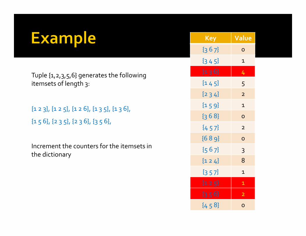
Tuple {1,2,3,5,6} generates the following
itemsets of length 3:
{1 2 3}, {1 2 5}, {1 2 6}, {1 3 5}, {1 3 6},
{1 5 6}, {2 3 5}, {2 3 6}, {3 5 6},
Increment the counters for the itemsets in
the dictionary
Key Value
{3 6 7} 0
{3 4 5} 1
{1 3 6} 3
{1 4 5} 5
{2 3 4} 2
{1 5 9} 1
{3 6 8} 0
{4 5 7} 2
{6 8 9} 0
{5 6 7} 3
{1 2 4} 8
{3 5 7} 1
{1 2 5} 0
{3 5 6} 1
{4 5 8} 0
Tuple {1,2,3,5,6} generates the following
itemsets of length 3:
{1 2 3}, {1 2 5}, {1 2 6}, {1 3 5}, {1 3 6},
{1 5 6}, {2 3 5}, {2 3 6}, {3 5 6},
Increment the counters for the itemsets in
the dictionary
Key Value
{3 6 7} 0
{3 4 5} 1
{1 3 6} 4
{1 4 5} 5
{2 3 4} 2
{1 5 9} 1
{3 6 8} 0
{4 5 7} 2
{6 8 9} 0
{5 6 7} 3
{1 2 4} 8
{3 5 7} 1
{1 2 5} 1
{3 5 6} 2
{4 5 8} 0
TID Items
1 Bread, Milk
2 Bread, Diaper, Beer, Eggs
3 Milk, Diaper, Beer, Coke
4 Bread, Milk, Diaper, Beer
5 Bread, Milk, Diaper, Coke
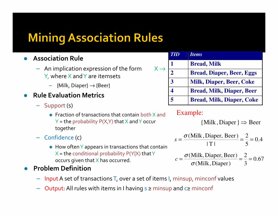
Example:
Beer}Diaper,Milk{ ⇒
4.05
2
|T|
)BeerDiaper,,Milk(===
σs
67.03
2
)Diaper,Milk(
)BeerDiaper,Milk,(===
σ
σc
� Association Rule
– An implication expression of the form X →Y, where X and Y are itemsets
– {Milk, Diaper} → {Beer}
� Rule Evaluation Metrics
– Support (s)
� Fraction of transactions that contain both X and
Y = the probability P(X,Y) that X and Y occur
together
– Confidence (c)
� How often Y appears in transactions that contain
X = the conditional probability P(Y|X) that Y
occurs given that X has occurred.
� Problem Definition
– Input A set of transactions T, over a set of items I, minsup, minconf values
– Output: All rules with items in I having s ≥ minsup and c≥ minconf

� Two-step approach:
1. Frequent Itemset Generation
– Generate all itemsets whose support ≥ minsup
2. Rule Generation
– Generate high confidence rules from each frequent
itemset, where each rule is a partitioning of a frequent
itemset into Left-Hand-Side (LHS) and Right-Hand-
Side (RHS)Frequent itemset: {A,B,C,D}
Rule: AB→CD

� Confidence is anti-monotone w.r.t. number of items on the RHS of the rule (or monotonewith respect to the LHS of the rule)
� e.g., L = {A,B,C,D}:
c(ABC → D) ≥ c(AB → CD) ≥ c(A → BCD)

� Candidate rule is generated by merging two rules that share the same prefixin the RHS
� join(CD→AB,BD→AC)would produce the candidaterule D → ABC
� Prune rule D → ABC if itssubset AD→BC does not havehigh confidence
� Essentially we are doing APriori on the RHS
BD->ACCD->AB
D->ABC


TID A1 A2 A3 A4 A5 A6 A7 A8 A9 A10 B1 B2 B3 B4 B5 B6 B7 B8 B9 B10 C1 C2 C3 C4 C5 C6 C7 C8 C9 C10
1 1 1 1 1 1 1 1 1 1 1 0 0 0 0 0 0 0 0 0 0 0 0 0 0 0 0 0 0 0 0
2 1 1 1 1 1 1 1 1 1 1 0 0 0 0 0 0 0 0 0 0 0 0 0 0 0 0 0 0 0 0
3 1 1 1 1 1 1 1 1 1 1 0 0 0 0 0 0 0 0 0 0 0 0 0 0 0 0 0 0 0 0
4 1 1 1 1 1 1 1 1 1 1 0 0 0 0 0 0 0 0 0 0 0 0 0 0 0 0 0 0 0 0
5 1 1 1 1 1 1 1 1 1 1 0 0 0 0 0 0 0 0 0 0 0 0 0 0 0 0 0 0 0 0
6 0 0 0 0 0 0 0 0 0 0 1 1 1 1 1 1 1 1 1 1 0 0 0 0 0 0 0 0 0 0
7 0 0 0 0 0 0 0 0 0 0 1 1 1 1 1 1 1 1 1 1 0 0 0 0 0 0 0 0 0 0
8 0 0 0 0 0 0 0 0 0 0 1 1 1 1 1 1 1 1 1 1 0 0 0 0 0 0 0 0 0 0
9 0 0 0 0 0 0 0 0 0 0 1 1 1 1 1 1 1 1 1 1 0 0 0 0 0 0 0 0 0 0
10 0 0 0 0 0 0 0 0 0 0 1 1 1 1 1 1 1 1 1 1 0 0 0 0 0 0 0 0 0 0
11 0 0 0 0 0 0 0 0 0 0 0 0 0 0 0 0 0 0 0 0 1 1 1 1 1 1 1 1 1 1
12 0 0 0 0 0 0 0 0 0 0 0 0 0 0 0 0 0 0 0 0 1 1 1 1 1 1 1 1 1 1
13 0 0 0 0 0 0 0 0 0 0 0 0 0 0 0 0 0 0 0 0 1 1 1 1 1 1 1 1 1 1
14 0 0 0 0 0 0 0 0 0 0 0 0 0 0 0 0 0 0 0 0 1 1 1 1 1 1 1 1 1 1
15 0 0 0 0 0 0 0 0 0 0 0 0 0 0 0 0 0 0 0 0 1 1 1 1 1 1 1 1 1 1
� Some itemsets are redundant because they have identical support as their supersets
� Number of frequent itemsets
� Need a compact representation∑
=
×=
10
1
103
k
k

Border
Infrequent
Itemsets
Maximal
Itemsets
An itemset is maximal frequent if none of its immediate supersets is frequent
Maximal itemsets = positive border
Maximal: no superset has this property

Border
Infrequent
Itemsets
Itemsets that are not frequent, but all their immediate subsets are frequent.
Minimal: no subset has this property

� Border = Positive Border + Negative Border
� Itemsets such that all their immediate subsets are
frequent and all their immediate supersets are
infrequent.
� Either the positive, or the negative border is
sufficient to summarize all frequent itemsets.

TID Items
1 {A,B}
2 {B,C,D}
3 {A,B,C,D}
4 {A,B,D}
5 {A,B,C,D}
� An itemset is closed if none of its immediate supersets has
the same support as the itemset
Itemset Support
{A} 4
{B} 5
{C} 3
{D} 4
{A,B} 4
{A,C} 2
{A,D} 3
{B,C} 3
{B,D} 4
{C,D} 3
Itemset Support
{A,B,C} 2
{A,B,D} 3
{A,C,D} 2
{B,C,D} 3
{A,B,C,D} 2

TID Items
1 ABC
2 ABCD
3 BCE
4 ACDE
5 DE
null
AB AC AD AE BC BD BE CD CE DE
A B C D E
ABC ABD ABE ACD ACE ADE BCD BCE BDE CDE
ABCD ABCE ABDE ACDE BCDE
ABCDE
124 123 1234 245 345
12 124 24 4 123 2 3 24 34 45
12 2 24 4 4 2 3 4
2 4
Transaction
Ids
Not supported
by any
transactions

null
AB AC AD AE BC BD BE CD CE DE
A B C D E
ABC ABD ABE ACD ACE ADE BCD BCE BDE CDE
ABCD ABCE ABDE ACDE BCDE
ABCDE
124 123 1234 245 345
12 124 24 4 123 2 3 24 34 45
12 2 24 4 4 2 3 4
2 4
Minimum support = 2
# Closed = 9
# Maximal = 4
Closed
and
maximal
Closed but not
maximal


� Association rule algorithms tend to produce too many rules but many of them are uninteresting or redundant� Redundant if {A,B,C} → {D} and {A,B} → {D} have same support &
confidence▪ Summarization techniques
� Uninteresting, if the pattern that is revealed does not offer useful information.▪ Interestingness measures: a hard problem to define
� Interestingness measures can be used to prune/rank the derived patterns� Subjective measures: require human analyst
� Objective measures: rely on the data.
� In the original formulation of association rules, support & confidence are the only measures used

� Given a rule X →Y, information needed to compute rule interestingness can be obtained from a contingency table
� ��
� f11 f10 f1+
�� f01 f00 fo+
f+1 f+0 N
Contingency table for X →Y
f11: support of X and Y
f10: support of X and Y
f01: support of X and Y
f00: support of X and Y
Used to define various measures
� support, confidence, lift, Gini,
J-measure, etc.
�: itemset X appears in tuple
�: itemsetY appears in tuple
��: itemset X does not appear in tuple
��: itemsetY does not appear in tuple

Coffee Coffee
Tea 15 5 20
Tea 75 5 80
90 10 100
Association Rule: Tea → Coffee
Confidence= P(Coffee|Tea) = �
��0.75
but P(Coffee) = �
����0.9
• Although confidence is high, rule is misleading
• P(Coffee|Tea) = 0.9375
Number of people that
drink coffee and tea
Number of people that
drink coffee but not tea
Number of people that
drink coffee
Number of people that
drink tea

� Population of 1000 students� 600 students know how to swim (S)
� 700 students know how to bike (B)
� 420 students know how to swim and bike (S,B)
� P(S∧B) = 420/1000 = 0.42
� P(S) × P(B) = 0.6 × 0.7 = 0.42
� P(S∧B) = P(S) × P(B) => Statistical independence

� Population of 1000 students� 600 students know how to swim (S)
� 700 students know how to bike (B)
� 500 students know how to swim and bike (S,B)
� P(S∧B) = 500/1000 = 0.5
� P(S) × P(B) = 0.6 × 0.7 = 0.42
� P(S∧B) > P(S) × P(B) => Positively correlated
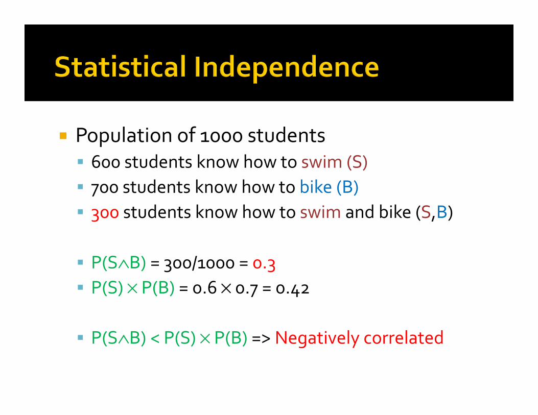
� Population of 1000 students� 600 students know how to swim (S)
� 700 students know how to bike (B)
� 300 students know how to swim and bike (S,B)
� P(S∧B) = 300/1000 = 0.3
� P(S) × P(B) = 0.6 × 0.7 = 0.42
� P(S∧B) < P(S) × P(B) => Negatively correlated

� Measures that take into account statistical dependence
� Lift/Interest/PMI
Lift � ���|��
�����
���, ��
� � ����� Interest
In text mining it is called: Pointwise Mutual Information
� Piatesky-Shapiro
PS � � �, � � � � ����
� All these measures measure deviation from independence� The higher, the better (why?)

Coffee Coffee
Tea 15 5 20
Tea 75 5 80
90 10 100
Association Rule: Tea → Coffee
Confidence= P(Coffee|Tea) = 0.75
but P(Coffee) = 0.9
⇒ Lift = 0.75/0.9= 0.8333 (< 1, therefore is negatively associated)
= 0.15/(0.9*0.2)

of the of, the
Fraction of
documents0.9 0.9 0.8
P�of, the� ! P of P�the�
If I was creating a document by picking words randomly, (of, the) have more
or less the same probability of appearing together by chance
hong kong hong, kong
Fraction of
documents0.2 0.2 0.19
P hong, kong ≫ P hong P�kong�
(hong, kong) have much lower probability to appear together by chance. The
two words appear almost always only together
obama karagounis obama, karagounis
Fraction of
documents0.2 0.2 0.001
P obama, karagounis ≪
P obama P�karagounis�
(obama, karagounis) have much higher probability to appear together by chance. The
two words appear almost never together
No correlation
Positive correlation
Negative correlation

honk konk honk, konk
Fraction of
documents0.0001 0.0001 0.0001
*� +,-., .,-. � 0.0001
0.0001 ∗ 0.0001� 10000
hong kong hong, kong
Fraction of
documents0.2 0.2 0.19
*� +,-3, .,-3 � 0.19
0.2 ∗ 0.2� 4.75
Rare co-occurrences are deemed more interesting.
But this is not always what we want