performance optimisation of vertical spindle coal pulverisers
TRANSCRIPT
\
Performance optimisation of vertical spindle coal pulverisers
SR Chateya
24668532
Dissertation submitted in fulfilment of the requirements for the degree
Master of Science in Engineering in Mechanical Engineering at the
Potchefstroom Campus of the North-West University
Supervisor: Prof CP Storm
November 2016
i
ABSTRACT
Coal pulverisers’ performance optimisation is an important process in power generation
plants. Pulveriser operation is costly; reliability and availability is key to power generation and
cost reduction is achieved by the optimal performance of associated plants. The objective of
this dissertation was to investigate the effect of coal feedstock property variation on the vertical
spindle coal pulverising mill’s performance to facilitate optimal plant performance. Plant design
and mill’s acceptance test data was analysed to understand the design and subsequent
changes over the years of the mill’s operation. The mill outputs, pulverised coal fineness and
distribution tests were carried out and evaluated from the data measured during plants tests.
A mathematical spreadsheet was used to observe mill performance when operating
parameters are varied. A mill’s heat balance evaluation was done using an Excel spreadsheet
to evaluate the mill drying capacity constraint. Coal analysis was done on hard grove grind
ability, abrasive indices and calorific value of coal. The effect of low calorific value coal was
observed on mill’s response to match the boiler energy requirements.
Evaluation of the current operating pulveriser data enabled the determination of the areas that
need improvement to achieve mill-optimal performance. Coal feed to the mill is important, this
was observed to be a limiting constraint on mill capacity when the coal required exceed
nominal load requirement.
KEYWORDS:
Air fuel ratio; pulverised fuel distribution; classifier; elutriation; heat balance; isokinetic
sampling; load line; mill throat; pulverisers; optimisation; pulverised fuel; recirculation; settling
velocity; models and control.
_______________________________
ii
OPSOMMING
Steenkool pulverisers se prestasie optimalisering is 'n belangrike proses in kragopwekking
plante. Pulveriser werking is duur; betroubaarheid en beskikbaarheid is die sleutel tot
kragopwekking en kostevermindering word bereik deur 'n optimale prestasie van
gepaardgaande plante. Die doel van hierdie verhandeling was om die effek van steenkool
roumateriaal eiendom variasie op die vertikale spil steenkool pulverising mill prestasie om
optimale plant prestasie te fasiliteer te ondersoek. Aanlegontwerp en Mill’s aanvaarding
SLEUTELTERME:
Air fuel ratio; pulverised fuel distribution; classifier; elutriation; heat balance; isokinetic
sampling; load line; mill throat; pulverisers; optimisation; pulverised fuel; recirculation; settling
velocity; models and control.
______________________________

iii
DECLARATION
I declare that this is my own work and that the work used here from others is referenced in the
thesis reference in-text and in the reference chapter.
……………………………………………
S.R. Chateya
Date
…………….……………………………..
______________________________

iv
DEDICATION
The thesis is dedicated to my wife Sylvia Dorcas and my two children, Kudzai Hazel and
Munashe Blessing Chateya.
______________________________

v
ACKNOWLEDGEMENTS
Professor CP Storm, my supervisor and mentor, for his guidance and encouragement during
the work on this dissertation. He had so much patience and resilience towards my study.
Thank you, Prof. Storm, you made a big difference in my life.
Secondly I would like to thank the Station management for allowing me to carry out a study
on the mills. Special thanks must go to Muzi Myeza and Sibusiso Nxumalo who encouraged
me to carry out a study on the mills with the view to optimising their performance .
Last, but not least, I would like to thank ESKOM for allowing this programme under further
studies and initially paying for this MSc programme for two years . To the North-West
University, Potchefstroom Campus, for allowing this research to be done, thank you.
Friends and relatives who kept me encouraged during the research period and those who also
provided literature and ideas - thank you very much, your presence made the difference. Prof
D J Simbi, a brother and friend who always encouraged me to embark on a postgraduate
study, thank you for the encouragement. Special thanks to Ramon Lopez ,Samuel Chizengeni
Jan Olivier , Hlono Malatsi,Simon Phala,and Mafhika Mkwanazi for their support during the
study.
My wife Sylvia Dorcas and my two children, Kudzai Hazel and Munashe Blessing Chateya are
warmly thanked for their support, patience and encouragement during the hard times of this
research.
To my children, your words of “Yes baba (father) it can be done” were a source of unwavering
encouragement.
To my dear wife Sylvia Dorcas, I will always be grateful for the time you made available for my
study on your home schedule.
I thank God for availing me this opportunity, which enabled me to interact with the above-
mentioned, and the strength to complete the study.
______________________________

vi
NOMENCLATURE
A Area in 𝑚2
Mc Coal flow kg/s
Ma Air flow kg/s
𝜌 Density kg/m3
g Constant of acceleration 9.81 m/s
∆𝑃 Differential pressure
M Mass flow kg/s
V Volumetric flow rate
v Velocity m/s
Cp Specific heat capacity kJ/kg.K
hf Enthalpy of saturated liquid kJ/kg
hfg Enthalpy of change phase (latent heat)
Tw Temperature at wall conditions
T Temperature at free stream conditions
W Power (kW)
HGI Hard grove grind ability index
Wi Bond work index
𝜇 Absolute viscosity
VSM Vertical spindle mill
𝑀𝑝𝑖𝑡𝑜𝑡 Pitot-mass flow as determined from a pitot traverse kg/s
Delta P Differential pressure across measuring device
Hg Enthalpy of saturated vapour kJ/kg
Im Inherent moisture %
Nsp Number of sampling points
P Pressure (Pa)
Pb Barometric pressure (Pa)
Ps Static pressure (Pa)
hv Dynamic pressure (Pa) velocity head pressure
sm Surface moisture %
T Temperature (K)
T Temperature (oC)
Tm Total moisture
I Number of mills in service
Qca Tempering air to the mill kg/s

vii
Qha Hot air to the mill Kg/s
Qsa Sealing air to the mill Kg/s
Ra Ideal gas constant for air, 287.04 J/kg.K
Tsa Temperature of sealing air (K)
I Mill drive current (A)
To Temperature of coal/air at mill outlet (K)
Vpf Pulverised coal air velocity m/s
___________________________________
viii
TABLE OF CONTENTS
ABSTRACT …………………………………………………………………………………..i
OPSOMMING…. ........................................................................................................... ii
DECLARATION ........................................................................................................... iii
DEDICATION ………………………………………………………………………………….iv
ACKNOWLEDGEMENTS ............................................................................................ v
NOMENCLATURE ....................................................................................................... vi
TABLE OF CONTENTS ............................................................................................. viii
LIST OF TABLES ....................................................................................................... xiv
LIST OF FIGURES .................................................................................................... xvi
1 INTRODUCTION ................................................................................... 1
1.1 Introduction ......................................................................................... 1
1.2 Problem statement .............................................................................. 1
1.3 Research aim ....................................................................................... 1
1.4 Scope of research ............................................................................... 2
1.5 Research background ......................................................................... 2
1.6 Outline of dissertation ........................................................................ 4
1.7 Conclusion........................................................................................... 5
2 LITERATURE SURVEY AND EXISTING TECHNOLOGY .................... 6
2.1 Introduction ......................................................................................... 6
2.2 Theories of comminution .................................................................... 6
2.2.1 Rittinger’s law ........................................................................................ 7
ix
2.2.2 Kick's law .............................................................................................. 7
2.2.3 Bond's law ............................................................................................. 8
2.2.4 The energy equation ............................................................................. 8
2.3 Hardgrove Grindability Index ............................................................. 9
2.3.1 HGI test procedure .............................................................................. 10
2.4 Abrasive Index ................................................................................... 11
2.5 Rosin and Rammler theory ............................................................... 11
2.6 Mill internal streams .......................................................................... 13
2.7 Mill operating window ....................................................................... 14
2.8 Mill operating parameters ................................................................. 16
2.8.1 Coal moisture ...................................................................................... 16
2.8.2 Mill inlet temperature ........................................................................... 16
2.8.3 Mill differential pressure ...................................................................... 17
2.8.4 Primary air differential pressure ........................................................... 17
2.9 Heat balance ...................................................................................... 18
2.10 Mill power consumption ................................................................... 19
2.11 Conclusion......................................................................................... 21
3 CHARACTERISATION OF VERTICAL SPINDLE COAL
PULVERISERS ................................................................................... 22
3.1 Introduction ....................................................................................... 22
3.2 Types of vertical spindle coal pulverisers ....................................... 22
3.3 Mill arrangement ............................................................................... 24
3.3.1 Mill coal feeder .................................................................................... 24
x
3.3.2 Seal air system .................................................................................... 25
3.3.3 Mill overview........................................................................................ 25
3.3.4 Mill throat area .................................................................................... 27
3.3.5 Primary air system............................................................................... 28
3.3.6 Grinding elements ............................................................................... 28
3.3.7 Mill pyrites rejecting system ................................................................. 29
3.4 Mill configuration .............................................................................. 29
3.5 Conclusion......................................................................................... 31
4 SIMULATION OF THE VERTICAL SPINDLE COAL PULVERISERS
EFFECTIVENESS ............................................................................... 32
4.1 Introduction ....................................................................................... 32
4.2 Research methodology overview ..................................................... 32
4.3 Plant design data analysis ................................................................ 32
4.4 Plant tests .......................................................................................... 33
4.4.1 PF sampling ........................................................................................ 33
4.4.2 Mill load simulations ............................................................................ 33
4.4.3 Hardgrove Grindability index ............................................................... 33
4.4.4 Abrasive Index .................................................................................... 34
4.4.5 Excel spreadsheet for mill performance evaluation.............................. 34
4.4.6 Heat balance ....................................................................................... 34
4.4.7 Conclusion .......................................................................................... 34
5 MILL DESIGN AND ACCEPTANCE TEST DATA .............................. 36
xi
5.1 Introduction ....................................................................................... 36
5.2 Mill and boiler design data ............................................................... 36
5.2.1 Mill design data ................................................................................... 36
5.2.2 Boiler design data ............................................................................... 37
5.3 Mill and boiler acceptance test data ................................................ 38
5.3.1 Mill acceptance data ............................................................................ 38
5.3.2 Boiler Specified Data acceptance data ................................................ 39
5.4 Discussion ......................................................................................... 40
5.5 Conclusion......................................................................................... 41
6 PLANT TESTS .................................................................................... 42
6.1 Introduction ....................................................................................... 42
6.2 Abrasive Index ................................................................................... 42
6.2.1 Abrasive Index test procedure ............................................................. 42
6.2.2 Abrasive Index test results .................................................................. 43
6.2.3 Abrasive Index test results discussion ................................................. 43
6.3 Hardgrove Grindability Index ........................................................... 44
6.3.1 Hardgrove Index test procedure .......................................................... 45
6.3.2 Hardgrove Grindability Index test results ............................................. 46
6.3.3 Hardgrove Index test results discussion .............................................. 48
6.4 PF sampling ....................................................................................... 48
6.4.1 PF sampling results ............................................................................. 49
6.4.2 PF sampling results ............................................................................. 50
xii
6.4.3 PF fineness results .............................................................................. 52
6.4.4 Mill pulverised fuel regression lines ..................................................... 54
6.4.5 Pulverised fuel Isokinetic sampling results discussion ......................... 58
6.5 Conclusion......................................................................................... 60
7 MILL POWER CONSUMPTION AND HEAT BALANCE EXCEL
SPREADSHEETS ............................................................................... 61
7.1 Introduction ....................................................................................... 61
7.2 Mill power consumption ................................................................... 61
7.3 Mill power consumption Excel spreadsheet results ....................... 61
7.3.1 Grinding table speed ........................................................................... 62
7.3.2 Primary air temperature ....................................................................... 63
7.3.3 Primary air pressure ............................................................................ 63
7.3.4 Number of balls in the mill ................................................................... 64
7.3.5 Grinding table coal feed rate ............................................................... 64
7.3.6 Mill grinding pressure .......................................................................... 65
7.3.7 Primary air flow ................................................................................... 65
7.3.8 Classifier blade angle setting ............................................................... 66
7.4 Mill power consumption Excel spreadsheet result’s discussion .. 67
7.5 Mill heat balance ............................................................................... 67
7.6 Mill heat balance Excel spreadsheet results. .................................. 67
7.7 Load simulations ............................................................................... 70
7.7.1 Discussion of results ........................................................................... 71
7.7.2 Conclusion .......................................................................................... 71
xiii
8 CONCLUSIONS AND RECOMMENDATIONS ................................... 72
REFERENCES .......................................................................................................... 76
APPENDICES............................................................................................................ 79
APPENDIX A: HARDGRAVE GRINDABILITY INDEX MACHINE (ACARP) ............. 79
APPENDIX C1: MILL A PF REGRESSION LINE ...................................................... 82
APPENDIX D: VALIDATION OF SIMULATED LOAD ............................................... 85
APPENDIX E: GRINDING TABLE FEED VS FRICTION FACTOR ........................... 86
APPENDIX F: GRINDING TABLE FEED VS FRICTIONAL FACTOR ....................... 87
APPENDIX I: CUT DIAMETER VS AIR FLOW .......................................................... 88
APPENDIX J: CUT VELOCITY VS PRIMARY AIR.................................................... 89
APPENDIX K: MILL POWER VS AIR FLOW ............................................................ 89
APPENDIX L: GRINDING TABLE FEED VS FRICTION FACTOR. .......................... 90
APPENDIX M: MILL FRICTIONAL FACTOR VS PRESSURE ON BALLS ............... 91
______________________________
xiv
LIST OF TABLES
Table 3.1: Mill arrangement schematic illustration of mill coal and air flow (Power Utility
X) .................................................................................................... 30
Table 5.1: Mill specified data ........................................................................... 36
Table 5.2: Boiler specified data ....................................................................... 37
Table 5.3: Mill particle size distribution ............................................................ 38
Table 5.4: Boiler guaranteed operation data .................................................... 39
Table 6.1: Abrasive Index test results .............................................................. 43
Table 6.2: Constants determination for HGI machine from standard reference
samples .......................................................................................... 44
Table 6.3: HGI test results for Power Utility coal .............................................. 46
Table 6.4: Mills test data .................................................................................. 49
Table 6.5: Mill calculated data ......................................................................... 51
Table 6.6: Pulverised fuel fineness results ....................................................... 53
Table 6.7: Results of a regression analysis for A. ............................................ 54
Table 6.8: Results of regression analysis for B ................................................ 55
Table 6.9: Result of regression analysis for C ................................................. 55
Table 6.10: Results of regression analysis for D ................................................ 56
Table 6.11: Results of regression analysis for E ................................................ 56
Table 6.12: Results of regression analysis for F ................................................ 57
Table 7.1: Mill power-draw results ................................................................... 62
Table 7.2: Grinding table speed results ........................................................... 62
Table 7.3: Primary air temperature .................................................................. 63

xv
Table 7.4: Primary air pressure ....................................................................... 63
Table 7.5: Number of mill balls ........................................................................ 64
Table 7.6: Grinding table coal feed .................................................................. 65
Table 7.7: Grinding pressure on mill balls ........................................................ 65
Table 7.8: Primary air flow rate ........................................................................ 66
Table 7.9: Classifier blade angle setting .......................................................... 66
Table 7.10: Mill heat balance Excel spreadsheet results ................................... 68
______________________________
xvi
LIST OF FIGURES
Figure 2.1: Rosin-Rammler graph .............................................................................. 12
Figure 2.2: Internal streams (Shi, 2011:59; Kojovic et al., 2015:602-611)................... 14
Figure 2.3: Mill operating window (Gill, 1984:339-353) ............................................... 15
Figure 3.1: Mill arrangement schematic illustration of mill coal flow and air flowl ........ 24
Figure 3.2: Table coal feeder (Power Utility X operating manual) ............................... 25
Figure 3.3: Mill sealing air arrangement ..................................................................... 26
Figure 3.4: Mill cross-section overview (Babcock 8.5 E-type). .................................... 27
Figure 3.5: Mill internal overview ................................................................................ 27
Figure 3.6: Hydraulic cylinder configuration (Lin and Penterson, 2004:6) ................... 29
Figure 4.1: Research methodology overview ............................................................. 32
Figure 6.1: Hardgrove testing machine cross section (ACARP 2008). ........................ 46
Figure 6.2: Power Utility HGI test results .................................................................... 47
______________________________
1
1 Introduction
1.1 Introduction
According to Singh (2011:1), 86% of South Africa’s electricity is generated from coal fuelled
power stations. A significant number of these power stations were designed to burn coal from
a dedicated coal mine. This minimised mill throughput and efficiency problems due to variation
of coal parameters.
Over the years the expansion of the coal market and the changes in price of coal resulted that
power stations use coal from different mines. The blending of coal from different suppliers has
resulted in noticeable coal quality variations from the design. The deviations from the designed
coal quality adversely impact power plant performance.
According to Etzinger (2013:1-10), Eskom initiated expansion of its generating fleet by building
new generation power stations Medupi and Kusile and returning to service the mothballed
power stations, namely, Grootvlei, Komati and Camden. The collieries that were dedicated to
supply these mothballed power stations remain closed. Thus new coal supplies were sourced,
resulting in significant challenges such as load losses and meeting desired mill throughput.
An investigation into the effect of coal feedstock property variation on the vertical spindle coal
pulverising mill performance has the potential to improve the performance of the power
stations.
1.2 Problem statement
Due to variation in the coal feedstock properties the coal pulverising mills at the Power Utility
are not operating optimally. This may have an effect on the fineness distribution of pulverised
fuel, pulverised fuel burner distribution, mill bias, mill throughput, mill outlet temperature,
power consumption, reliability and pulverised fuel settling velocity. It is currently not clear to
what extent this variation in feedstock properties influences a mill’s performance and product.
1.3 Research aim
The aim of this research project is to investigate the effect of coal feedstock property variation
on the vertical spindle coal pulverising mill’s performance to facilitate optimal plant
performance. This implies that research undertaken was a means to:
2
a. evaluate the current state of technology with regards to comminution of current coal
feed stock and compare with the equivalent initial design data;
b. assess the current plant performance of the mills under investigation;
c. develop a mathematical tool that may be used to optimise plant performance;
d. evaluate plant performance with the aim to optimise; and
e. conclude and make recommendations with regards to optimal plant operation.
1.4 Scope of research
To address the aims as presented above the scope is outlined as follows:
a. conduct a detailed literature review that establishes the current state of technology as
relevant to coal pulverisation technology, with specific emphasis on the vertical spindle
mills at Power Utility;
b. conduct plant tests at Power Utility X Unit 4 Mills A-E to evaluate plant performance
as related to fineness distribution of pulverised fuel, pulverised fuel burner distribution,
mill bias, mill throughput, mill outlet temperature, power consumption, reliability and
pulverised duel settling velocity;
c. conduct laboratory experimentation to determine coal fineness, calorific value,
hardgrove grindability index, abrasiveness index, ash and moisture content;
d. develop a mathematical model in Excel that simulates mill performance as a function
of variable coal feedstock properties and basic plant operation parameters;
e. optimise plant performance based on the mathematical model and tests through
evaluation of coal parameters and mill throughput; and
a. conclude and make recommendations on the current operational efficiency of the coal
pulveriser mills at Power Utility X Unit 4 Mill A-F and how they may be optimised.
1.5 Research background
Coal fuelled power stations use pulverised fuel in order to achieve optimum combustion and
ease of control. Coal is pulverised to obtain a noticeable increase in specific area per unit
mass, thus promoting efficient combustion when mixed with air. Increase in coal specific areas
due to pulverisation widens the choice of coal type that can be used in the power stations,
such as lignite, bituminous coal, anthracite, coke and even peat (Association & Field,
1967:175-231).
The performance of vertical spindle coal mills is considerably affected by variation in feedstock
quality, such as coal particle size, moisture content, calorific value, ash content, hardgrove

3
grindability index and Abrasive Index. The mill has four main functions, namely: grinding,
drying, transporting and classification of the pulverised coal.
The performance of the mill significantly impacts the burner efficiency and thus the energy
output of the burners. The pulverised coal fineness significantly impacts the performance of
the burners. Mill product with coarse particles results in noticeable incomplete combustion in
the burner.
The primary air supplied from the air pre-heater to the mill dries and transports the pulverised
coal to the burners. The design mill inlet and outlet temperature is 245oC and 85oC
respectively. The distribution of pulverised fuel to the burners is configured in such a way that
an equal mass of pulverised coal is split into equal masses to exit into the burners.
The temperature difference between the mill’s primary air temperature and the pulverised fuel
air temperature at mill outlet indicate the mill drying capacity. The mill receives the raw coal of
a particular size and of a specific moisture content. At Power Utility X , total moisture content
of the coal is around 10%.
Power Utility X has six units, Unit One to Unit Six, rated at 220 MW capacity. Each unit is
powered with five vertical spindle coal mills to achieve the design full load.
To maintain fluctuations in energy demand, the unit operator manually sets the mill load to
respond up or down. Three mills are set to increase coal feed when an increase in load is
required. The two mills are also set to decrease coal flow when load reduction is required on
the unit. This process is called ‘biasing’. Mill combination is another parameter that influences
the energy output from the furnace.
Mill capacity is the throughput the mill is able to deliver at the required unit load. Power Utility
mills have a designed throughput of 25 480 kg/hr of coal, which translates to 7.07 kg/s. The
total coal delivered to the unit for the five mills is 30 kg/s rated on design coal calorific value.
Mill power consumption affects the amount of auxiliary power for the power station unit. Power
Utility X units are rated at 220 MW each. The power station unit auxiliary power consumption
is designed at seven percent of the total generation. Thus, mill power consumption is a critical
parameter in the overall performance of the power station. Mill power usage above design
value has a negative impact on energy sent out by the unit. The other effect is that the auxiliary
power consumption affects the plant heat rate and efficiency.
When velocity drops as the air-pulverised fuel mixture travels along the pipes, coarse particles
tend to segregate around bends and form layers on parts of pipes with reduced velocity. The
4
velocity at which the segregation starts is called the ‘settling velocity’. Operating mills at
velocities lower than settling velocity causes pulverised fuel settling in pipes. This might result
in coal ignition in the pipes due to the continuous passing of hot air on stationary fuel.
Determination of pulverised fuel air mixture velocity is critical in minimising the chance of flash-
back and blow-off of flames on the burners. Flashback occurs when combustion velocity is
faster than fuel flow velocity; blow-off occurs when fuel flow velocity is faster than combustion
or burning velocity at the burner. This results in the injected coal not igniting.
The objective of maintaining mills is to maintain the capability of the mills while controlling
costs. Maintenance of the mills seeks to keep the equipment in working order while reliability
is the probability that the equipment will function properly for a specified time.
To improve the reliability of the mill, the maintenance strategy requires a focus upon individual
components such as the mill balls and the grinding rings. Implementing and improving
preventive maintenance significantly increases the availability of the mills.
The process of achieving pulverised fuel has noticeable costs, thus optimisation of the process
can significantly contribute to minimising operating costs.
1.6 Outline of dissertation
The dissertation consists of eight chapters, and each chapter focuses on a specific area of
investigation in the vertical spindle milling plant performance optimisation. This section gives
a brief summary of the chapters in the dissertation.
Chapter 1: This chapter introduces the dissertation, the objectives of the investigation, and
the limitations of the study. The chapter also covers the research proposal to motivate the
need for this research and clearly defines the scope of the research project. This chapter also
serves as a guide during the research process to ensure that the objective of the study is
achieved. The chapter presents an introduction to the investigation, the background and the
problem statement for the research project.
Chapter 2: This chapter presents the literature review and available technology for similar
work that has been done in vertical spindle coal pulveriser performance optimisation.
Chapter 3: This chapter gives details of the engineering design of vertical spindle coal
pulverisers and is the characterisation of vertical spindle pulverisers.
5
Chapter 4: This chapter deals with the methodology adopted in this research to carry out mill
performance optimisation tests, both at the power station and at the University facilities. The
results obtained from the tests should be applicable to any vertical spindle coal mills and
achieve performance optimisation.
Chapter 5: The chapter deals with the analysis of the mill and boiler design and acceptance
data to identify design changes over the mill operation.
Chapter 6: This chapter details the plant tests carried out to investigate the mill performance.
Chapter 7: This chapter details mill power consumption and heat balance Excel spreadsheets.
Chapter 8: This chapter provides the conclusions and recommendations drawn from the
results of the research. The recommendations and future work that can be done in the coal
mills performance optimisation to improve combustion efficiency.
1.7 Conclusion
Against the background given in this chapter, the purpose of this dissertation is defined as the
investigation of the effect of coal feedstock property variation on the vertical spindle coal
pulverising mill performance to facilitate performance optimisation of vertical spindle coal
pulverisers.
This chapter presented the introduction, the problem statement, aim of the research, scope of
the research, research background and dissertation outline. The next chapter focuses on the
literature review that establishes the current state of technology as relevant to coal
pulverisation.
6
2 Literature survey and existing technology
2.1 Introduction
The aim of this study is to perform an investigation on the effect of coal feedstock property
variation on the vertical spindle coal pulverising mill performance to facilitate optimal plant
performance. This chapter focuses on a detailed literature review that establishes the current
state of technology as relevant to coal pulverisation technology with specific emphasis on the
vertical spindle mill’s at Power Utility X Unit 4.
The chapter presents an overview on the theories of comminution in Section 2.2 and
hardgrove grindability in Section 2.3. This is followed by the Abrasive Index in Section 2.4 and
Rosin and Rammler Theory in Section 2.5. A discussion of mill internal streams (Section 2.6)
and mill operating parameters (Section 2.7), as well as mill models and controls (Section 2.8)
trails. The chapter ends with a conclusion in Section 2.9.
2.2 Theories of comminution
Comminution of solids in to fine powder in the industry involves a process of grinding,
classification and further size reduction until the required size is achieved. The process of
grinding is expensive if proper monitoring and plant optimisation are not implemented (Rubiera
et al.,1999). In some industries the grinding process becomes prohibitively costly, to the point
where the final product is not price-competitive. This section will emphasise theories of
comminution relevant to vertical spindle coal mills.
When the high cost persists, business continuation may be hampered, hence the need to
reduce operational costs. The way to reduce costs is by understanding the cost of grinding
and analysing the areas that need optimising in order to reduce costs. The comminution
process involves the provision of material to be ground, as well as the state of the grinding
components. The optimisation is meant to extend the life of the grinding components and
improve the pulverised coal throughputs (Walqui et al., 2003; Kawatra & Eisele, 2005).
The coal pulverisation process is significantly costly as the grinding mills wear/replacements
costs escalate. Companies dealing in powder products have tried to reduce the grinding costs
of these processes. The mill manufacturers have been involved in wear research of mill
grinding components with the aim of reducing and understanding the grinding processes to
ultimately extend grinding components’ life.
7
Rittinger, Bond and Kick came up with theoretical and empirical energy size reduction
equations and these became known as the three laws of comminution (Rittinger, 1867; Bond,
1952; Kick, 1855). Further work by Walker (1937) and Hukki (1962) resulted in the combination
of the three laws to give an energy relationship during comminution. The three empirical
grinding energy relationships are defined in the energy requirements. The laws of comminution
are summarised as:
Rittinger's law, which assumes that the energy consumed is proportional to the newly-
generated surface area; it is considered to be the first law of comminution;
Kick's law, which relates the energy to the sizes of the feed particles and the product
particles, the second law of comminution;
Bond's law, which assumes that the total work useful in breakage is inversely
proportional to the square root of the diameter of the product particles, implying
theoretically that the work input varies as the length of the new cracks are made in
breakage, the third law of comminution; and
Holmes's law, which modifies Bond's law by substituting the square root with an
exponent that depends on the material.
2.2.1 Rittinger’s law
Rittinger’s law states that during grinding the work done is proportional to the new surface
created during the grinding process (Rittinger, 1879). The size of the solids entering the mill
is continuously reduced to achieve the required size. Significant amounts of energy are used
to achieve the desired particle size. According to Rittinger (1867) the work done is proportional
to the energy used.
Rittinger’s law is mathematically expressed as follows:
𝑬 = 𝑪 (𝟏
𝑫𝒑−
𝟏
𝑫𝒇) 2.1
where E = energy required, C = a constant, Dp = 80% passing size product and Df = passing
size of feed.
2.2.2 Kick's law
Kick’s law states that during grinding the work done is proportional to reduction in volume
(Kick, 1885). Equation 2.2 mathematically expresses Kick’s law.
8
𝑬 = 𝑪. 𝒍𝒐𝒈 (𝑫𝒇
𝑫𝒑) 2.2
where E = energy required, C = a constant, Dp = 80% passing size product and Df = 80%
passing size of feed.
This implies that the grinding rate is independent of particle size because it is based on a
constant as well as a reduction ratio. Equal amounts of energy would be required to achieve
size reductions regardless of particle size.
2.2.3 Bond's law
On analysing the laws that govern grinding, another important law was proposed by Bond
(1952). The law is known as Bond's Third Theory. Bond postulated that work done during
grinding is proportional to the new crack-tip length produced. Equation 2.3 shows Bond’s law.
𝑬 = 𝑪 (𝟏
√𝑷𝟖𝟎−
𝟏
√𝑭𝟖𝟎
) 2.3
where E = energy required, C = a constant, P80 = 80% passing size product and F80 = 80%
passing size feed.
Bond’s law was considered to be in-between Kick's and Rittinger's and this is shown in
Equation 2.4.
𝑾 = 𝟏𝟎 𝑾𝒊
√𝑷𝟖𝟎−
𝟏𝟎𝑾𝒊
√𝑭𝟖𝟎 2.4
where W = work output (kWh/t), W i = work index, P80 = 80% passing size product and F80 =
80% passing size of feed.
2.2.4 The energy equation
Rittinger, Kick and Bond’s laws can be combined into the general form of a comminution
energy equation, shown in Equation 2.5 (Hukki, 1961; Jankovic et al., 2010:1-10).
𝒅𝑬 = −𝑪 𝒅𝒙
𝒙𝒏 2.5
where E = net specific energy, x = characteristic dimension of the product, n = the exponent
and C = constant related to material.
9
Equation 2.5 shows that the required energy for a differential decrease in size is proportional
to the size change (dx) and inversely proportional to the power n.
When Equation 2.5 is integrated and exponent n given values of 2, 1 and 1.5, the three laws
of comminution equations are obtained.
The comminution laws are usable to the evaluation of energy consumption in the grinding
processes, as solid materials are being reduced to fine grinding. In power stations coal needs
to be pulverised to a fine powder for ease of combustion in the burners.
The mill power draw is important and parameters that contribute to high mill power-draw have
to be monitored in order to reduce a high power-draw, which can power-draw increase the
auxiliary power consumption on a running plant. The high auxiliary power consumption has a
negative impact on the increase of the heat rate on the running unit, as this power consumption
is included in the calculation of the heat rate.
High heat rate means that high energy is required for power generation, creating a reduction
in efficiency as input increases more than design energy requirements. Due to the high impact
of energy usage during solids grinding and size reduction, it is very important that the grinding
process and mechanisms be understood and optimum running achieved in order to run
economically.
Reliability and Power-plant Performance engineers use these laws to formulate programmes
that are used to monitor the efficiency and reliability of grinding plants. The knowledge of the
coal’s physical properties that affect comminution should be understood and their effect
evaluated.
The physical coal properties that are considered in coal comminution are the Hardgrove
Grindability Index, Abrasiveness Index and the coal strength (Speight, 2015:155-165; Sligar,
1996:569-581; Sligar, 1998)
2.3 Hardgrove Grindability Index
Coal pulveriser output is rated through the use of the Hardgrove Grindability Index (HGI). Mill
outputs are rated according to how hard or soft the coal is and the parameter used is the HGI.
HGI is the coal property that describes how soft or hard the coal is to grind. The measure is
on a scale of 0-100. The mill manufacturers give an HGI of 50-60 for a particular mill and if the
coal changes to an HGI above 50, the coal is getting softer and, vice versa, a lower HGI means
the coal is getting harder to grind (Sligar, 1998:1-8)
10
The HGI developed by Hardgrove is intended to measure empirically the relative difficulty of
grinding coal to the particle size necessary for relatively complete combustion. This was used
in the then newly-developed pulverised coal boiler furnace. Its use has been extended to
grinding coal for the iron-making, cement and chemical industries utilising coal (Tichanek,
2008:27-32; ACARP, 1998:1-8).
More recently it has acquired another role as one of the properties of specification when
purchasing coal from different potential suppliers. The specification usually lists a range of
values for every property within which the plant is known to function efficiently. These values
may arise from the original design or from practical experience with a specific plant.
2.3.1 HGI test procedure
According to ACARP (1998:1-8), HGI test is done using a small pulverising machine which
resembles a Babcock E-type vertical spindle coal mill. The test coal is air-dried and of a
specific size, and the HGI test resembles the operation of a ball and track type of industrial
coal pulveriser manufactured by Babcock. The test is accomplished by taking batch samples
with specified sizes.
A 50g sample of coal, which has been prepared in a specific manner with a limited particle
size range (1.18 x 0.6 mm), is placed in a stationary grinding bowl. The grinding bowl has eight
steel balls which run in a circular path. A loaded ring is placed on top of the set of balls with a
gravity load of 284 N. The machine is run for 50 revolutions.
The grounded coal is graded according to the sizes passing through a 75 Microns Sieve. The
coal less than 75 microns recorded is converted to an HGI value using a calibration graph.
The HGI test standards differs from one country to another. These differences are well
understood by boiler and coal pulveriser designers but have led to noticeable confusion when
used commercially for coal trading. The method of preparing samples before the test poses
significant variances in standards.
The characteristics of the HGI are (ACARP, 1998:1-8, Hower, 1990):
an empirical test not linked with a known physical property of coal;
exhibits a non-linear change in difficulty to grind; and
it is not additive.
11
Coal with low values of HGI is significantly difficult to grind, while high HGI values are easier
to grind. Thus, a mill designed to crush coal with an HGI of 60 when used with lower HGI
values is harder coal, while an HGI value of above 60 means softer coal (ACARP, 1998:1-8,
Hower, 1990).
2.4 Abrasive Index
The coal-grinding process results in wear of grinding components due to the grounded
material’s hardness. The loss in weight of material from initial mass to the final mass is a
measure of the abrasiveness of the material being handled.
The life of pulverised coal handling equipment depends on the errosiveness of the coal being
used (Speight, 2005:155-165). The wear rate of grinding components depends on the
hardness of the material in use and the amount of air being handled by the mill (Gill, 1984:343-
361).
The Yancey Gear Price Index is used for the abrasiveness index determination. The tests are
done on a batch system but applying this to real plant results may be different, due to the
conditions encountered during operations.
The mill has a hydraulic pressure system that presses on the grinding ring. The grinding
maintains a specified clearance between the rings and the balls. This gap prevents any metal
to metal contact of the balls and rings. The wear rate of grinding elements is due to the
abrasiveness character of coal during the coal pulverisation process.
Equation 2.6 shows the relationship between wear rate and the mill grinding pressure (Sligar,
1995). Equation 2.6 has a correlation coefficient of 82% (Sligar, 1995; Scott, 1995:42-44).
Equation 2.6 was modified to Equation 2.7 to give improved results.
𝑾𝒆𝒂𝒓 𝒓𝒂𝒕𝒆 = 𝟏. 𝟐𝟒 × 𝒈𝒓𝒊𝒏𝒅𝒊𝒏𝒈 𝒑𝒓𝒆𝒔𝒔𝒖𝒓𝒆 + 𝟎. 𝟕𝟕 2.6
𝑾𝒆𝒂𝒓 𝒓𝒂𝒕𝒆 = 𝟎. 𝟏𝟕 × 𝑨𝒃𝒓𝒂𝒔𝒊𝒐𝒏 𝒊𝒏𝒅𝒆𝒙(𝒈𝒓𝒊𝒏𝒅𝒊𝒏𝒈 𝒑𝒓𝒆𝒔𝒔𝒖𝒓𝒆 + 𝟏. 𝟖) × 𝟗𝟕% 2.7
2.5 Rosin and Rammler theory
According to Association and Field (1967:245-249), the milling of coal produces a powder
containing particles in a wide range of sizes. Theoretical analysis of combustion must take
account of the particle size distribution of the fuel, and the application of the theoretical results
demands a knowledge of the fineness of fuels in industrial use. In power plants’ various
12
technologies of milling plants are employed and the fineness may depend on the type of mill
in use. The mill performance is monitored by analysing the fineness of coal produced by the
grinding mill (Association & Field, 1967:245-249).
The grinding process aims to achieve a specified fineness to enable usage of the product.
Further work has been done to improve upon the formulation of the relationship between
comminution and the energy used to grind the particles to the required size.
After the grinding of the solids into powder, the product is assessed in terms of the suitability
of the fineness. In power stations, the mills are monitored by isokinetic-taking representative
samples from the exit of the mill. The samples are mechanically sieved and graded to give
data that represent particle size distribution (Association & Field, 1967:245).
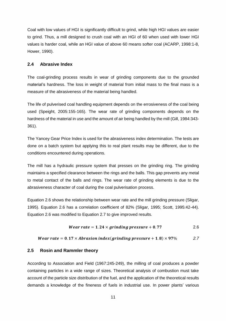
The frequently used method of analysing the particle size is by plotting the sieving results on
the Rosin-Rammler graph. Figure 2.1 shows the standard Rosin-Rammler graph. The
distribution of particle sizes follows an exponential law shown in Equation 2.8 (Association &
Field, 1967:245; Rosin and Rammler, 1933:29-36).
Figure 2.1: Rosin-Rammler graph
99.99
99.95
99.9
99.5
99
95
90
85
80
75
70
65
60 75 106 150 300 500
Mas
s F
ract
ion
Pas
sing
(%)
Sieve Size (µm)
13
𝑹𝒅 = 𝟏𝟎𝟎𝒆−𝒃𝒅𝒏 2.8
Taking the natural logarithm of the Equation 2.8, which results in a log-log graph plot that will
give a straight line of the powder particle distribution. This is shown in Equation 2.9.
𝒍𝒐𝒈 (𝒍𝒐𝒈𝟏𝟎𝟎
𝑹𝒅) = 𝒏. 𝒍𝒐𝒈𝒅 + 𝒍𝒐𝒈𝒄 2.9
The graphic representation of the particle distribution is important for decision-making with
regards to mill performance. The isokinetic sampling of pulverised coal is done in order to
determine true representation. The graph is affected by plant operations that affect the
coarseness and fineness of the pulverised powder going to the burners for combustion to take
place.
2.6 Mill internal streams
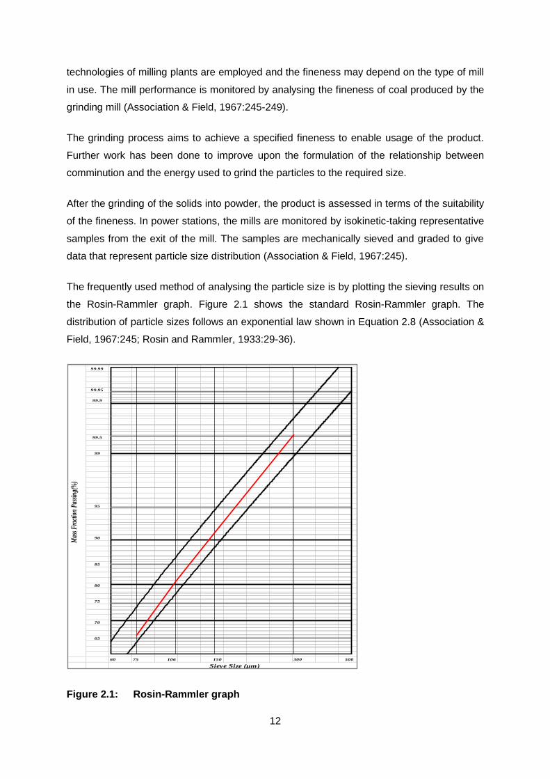
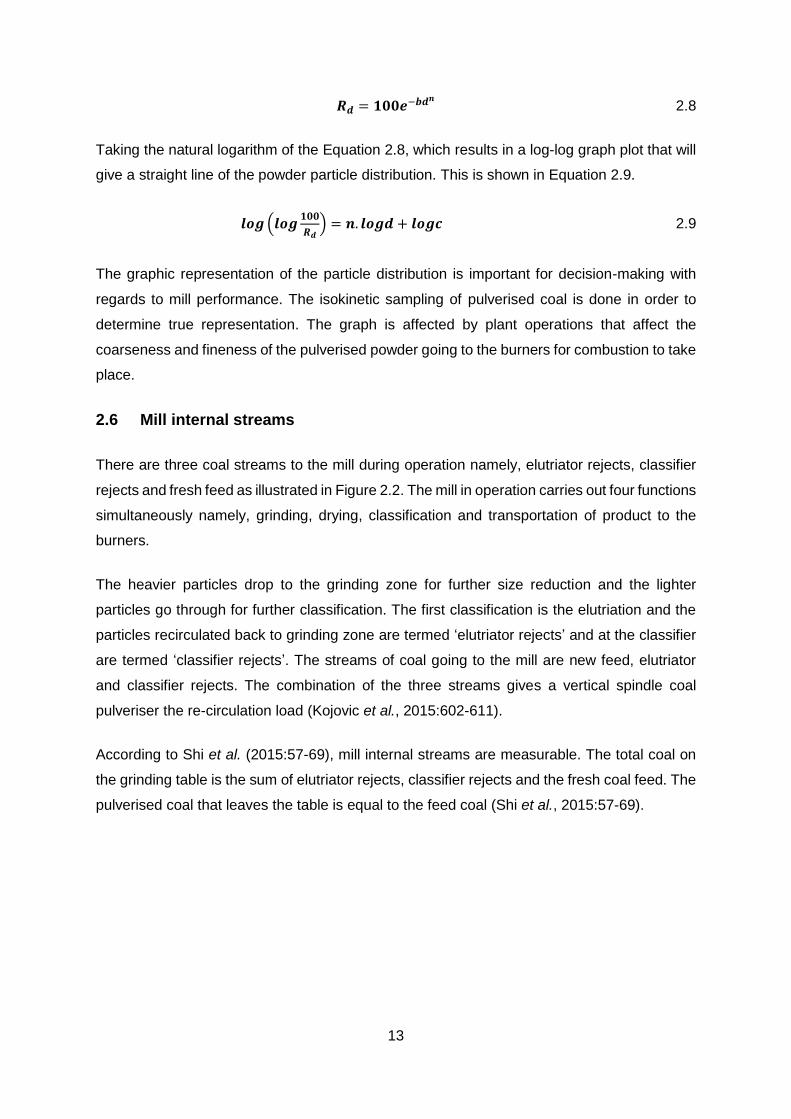
There are three coal streams to the mill during operation namely, elutriator rejects, classifier
rejects and fresh feed as illustrated in Figure 2.2. The mill in operation carries out four functions
simultaneously namely, grinding, drying, classification and transportation of product to the
burners.
The heavier particles drop to the grinding zone for further size reduction and the lighter
particles go through for further classification. The first classification is the elutriation and the
particles recirculated back to grinding zone are termed ‘elutriator rejects’ and at the classifier
are termed ‘classifier rejects’. The streams of coal going to the mill are new feed, elutriator
and classifier rejects. The combination of the three streams gives a vertical spindle coal
pulveriser the re-circulation load (Kojovic et al., 2015:602-611).
According to Shi et al. (2015:57-69), mill internal streams are measurable. The total coal on
the grinding table is the sum of elutriator rejects, classifier rejects and the fresh coal feed. The
pulverised coal that leaves the table is equal to the feed coal (Shi et al., 2015:57-69).
14
Figure 2.2: Internal streams (Shi, 2011:59; Kojovic et al., 2015:602-611).
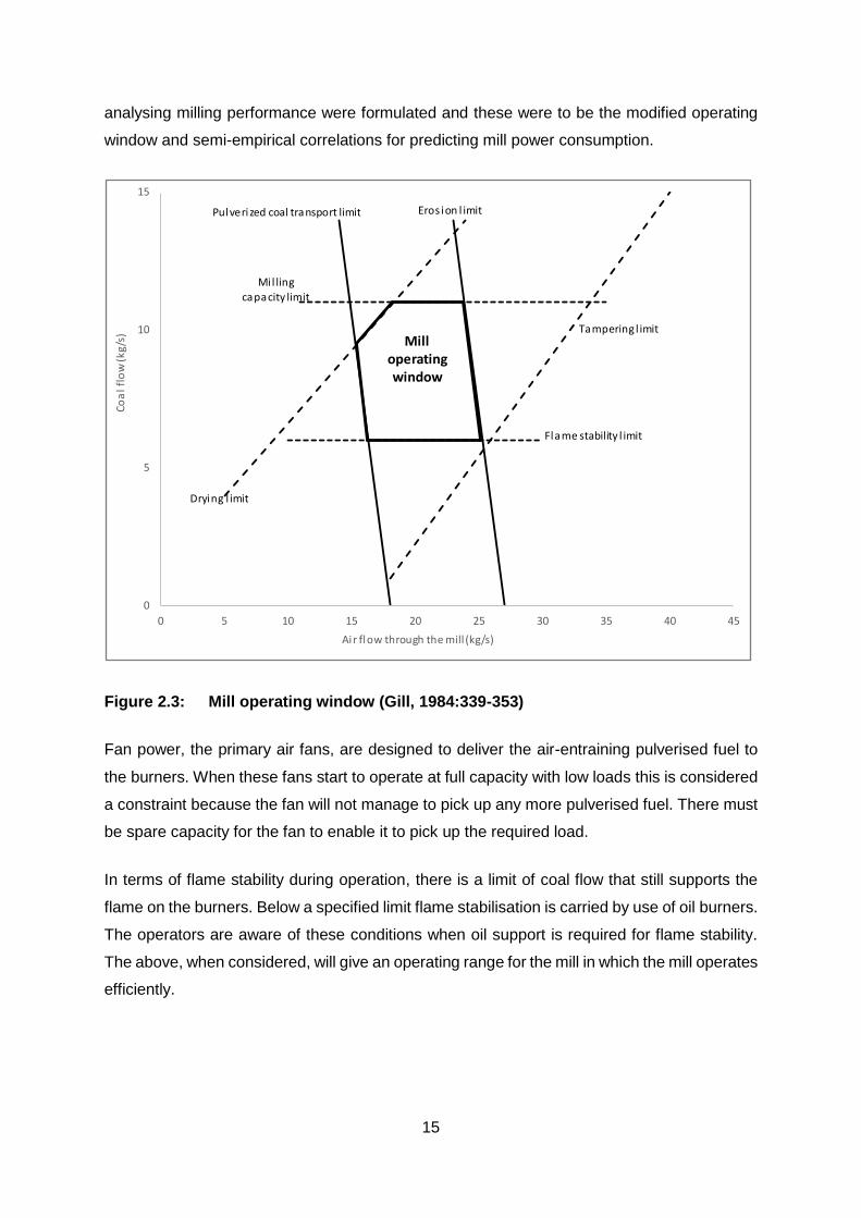
2.7 Mill operating window
According to Gill (1984: 339-353), mill operating parameters are considered for the mill to
achieve acceptable fineness and load. The parameters when considered will give a graphical
representation of the mill operating window. The mill operating window is plotted using the mill
operating parameters, such as: drying limit, erosion limit, milling capacity limit, tampering limit,
flame stability limit and pulverised coal transport (Gill, 1984:339-353). Figure 2.3 shows the
mill operating window.
The operating window provides the limits in which a mill best operates outside of when
constraints are experienced (Gill, 1984:339-353).
Arauzo and Cortes (1995), further explored the diagnosis of milling systems’ performance
based on the operating window and mill power consumption correlation. Procedures for
15
analysing milling performance were formulated and these were to be the modified operating
window and semi-empirical correlations for predicting mill power consumption.
Figure 2.3: Mill operating window (Gill, 1984:339-353)
Fan power, the primary air fans, are designed to deliver the air-entraining pulverised fuel to
the burners. When these fans start to operate at full capacity with low loads this is considered
a constraint because the fan will not manage to pick up any more pulverised fuel. There must
be spare capacity for the fan to enable it to pick up the required load.
In terms of flame stability during operation, there is a limit of coal flow that still supports the
flame on the burners. Below a specified limit flame stabilisation is carried by use of oil burners.
The operators are aware of these conditions when oil support is required for flame stability.
The above, when considered, will give an operating range for the mill in which the mill operates
efficiently.
0
5
10
15
0 5 10 15 20 25 30 35 40 45
Co
al
flo
w (
kg/s
)
Ai r flow through the mill (kg/s)
Mi l ling capacity limit
Pulverized coal transport limit
Drying l imit
Flame stability l imit
Tampering l imit
Eros ion l imit
Mill operating window
16
2.8 Mill operating parameters
2.8.1 Coal moisture
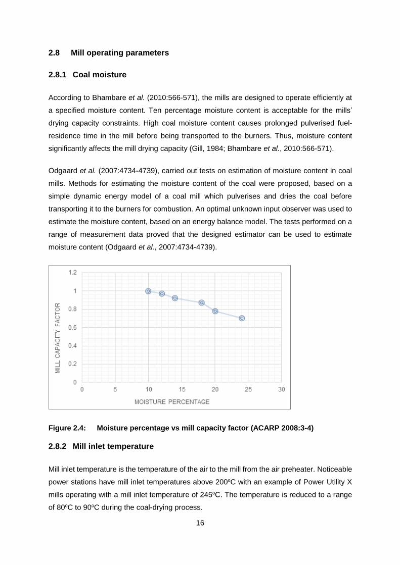
According to Bhambare et al. (2010:566-571), the mills are designed to operate efficiently at
a specified moisture content. Ten percentage moisture content is acceptable for the mills’
drying capacity constraints. High coal moisture content causes prolonged pulverised fuel-
residence time in the mill before being transported to the burners. Thus, moisture content
significantly affects the mill drying capacity (Gill, 1984; Bhambare et al., 2010:566-571).
Odgaard et al. (2007:4734-4739), carried out tests on estimation of moisture content in coal
mills. Methods for estimating the moisture content of the coal were proposed, based on a
simple dynamic energy model of a coal mill which pulverises and dries the coal before
transporting it to the burners for combustion. An optimal unknown input observer was used to
estimate the moisture content, based on an energy balance model. The tests performed on a
range of measurement data proved that the designed estimator can be used to estimate
moisture content (Odgaard et al., 2007:4734-4739).
Figure 2.4: Moisture percentage vs mill capacity factor (ACARP 2008:3-4)
2.8.2 Mill inlet temperature
Mill inlet temperature is the temperature of the air to the mill from the air preheater. Noticeable
power stations have mill inlet temperatures above 200oC with an example of Power Utility X
mills operating with a mill inlet temperature of 245oC. The temperature is reduced to a range
of 80oC to 90oC during the coal-drying process.
17
According to Niemczyk (2010:32-36), the coal and air flow thermodynamic and hydrodynamic
effects must be considered when modelling vertical spindle coal mills. The mill is supplied with
hot air from the air preheater to heat and dry the coal during conveyance to the burners. The
temperature of the primary air is noteworthy in the evaluation of the drying capacity of the mill
(Niemczyk, 2010:32-36).
During operation there is pressure drop across the mill as coal enters the mill and is ground
during the plant operation. A fraction of coal is transferred to the elutriator via hot air during
grinding and a fraction remains on the grinding table for further pulverisation. This balance has
to be maintained for continuous operation of the plant.
2.8.3 Mill differential pressure
The amount of recirculation load in the mill at any time is indicated by the pressure drop across
the mill. This pressure drop is called the mill differential pressure. The change in the mill
differential pressure has a relation to how much coal is circulating in the mill during the grinding
process. The circulating coal during the load is termed ‘re-circulating load’ and the relationship
is evaluated using differential pressure.
The primary air is directed through the mill to dry the coal and convey the dry pulverised fuel
to the burners. The amount of coal in the mill causes resistance to the flow of coal, setting up
the differential pressure across the mill.
The differential pressure is used to control the amount of coal circulating at any particular time.
The mill-differential pressure versus the primary air-differential pressure gives a graph that is
used as a load line. The load line is the relationship between the coal flow and the air flow. In
normal operations of the mill the load line represents the air and fuel ratios. The air/fuel ratios
are used to evaluate air flows to the mill and to the boilers when coal flow is known.
2.8.4 Primary air differential pressure
The primary air measurement is done by a measuring device called a Venturi also known as
‘orifice’. The differential pressure across the primary air measuring instrument indicates the
amount of air flowing across the instrument to the coal mills. The primary air differential
pressure is the measure of air flow to the mill.
A graphic relationship is used to indicate the air flow to the mill versus the opening of air vanes
on the primary air fan. The vane openings are calibrated using the pitot tube traverse data to
18
evaluate the amount of air passing at a vane opening. A graph of vane opening percentage
versus air flow is plotted and is used as a performance monitoring tool.
2.9 Heat balance
The mill heat balance is evaluated using Equation 2.10 to Equation 2.21. These equations are
derived from Fan and Rees’s proposed equations. (Fan & Rees, 1994:235). Equation 2.10 to
Equation 2.14 shows the mill energy input.
𝑸𝒆𝒄𝒊 = (𝟏 − 𝑾𝒕𝒎)𝑪𝒑𝒄𝑴𝒄𝒇(𝑻𝒄𝒕 − 𝑻𝒂) 2.10
where Qeci = energy of coal in, Cpc = specific heat coal, Mcf = coal flow rate, Tct = coal
temperature, Ta = ambient temperature and Wtm= total percentage moisture of coal.
𝑸𝒆𝒎𝒊 = 𝑾𝒕𝒎 × 𝑴𝒄𝒇 × 𝑯𝒇𝒊 2.11
where Qemi = energy of moisture in, Mcf = mass of raw coal and Hfi = enthalpy of saturated
liquid at mill inlet.
𝑸𝒆𝒑𝒂𝒊 = 𝑴𝒑𝒂 × 𝑪𝒑𝒂(𝑻𝒑𝒂𝒕 − 𝑻𝒂) 2.12
where Qepai = energy of primary air in, Mpa = primary air flow rate, Tpat = temperature of primary
air, Cpa = specific heat capacity of air.
𝑸𝒆𝒔𝒂𝒊 = 𝑴𝒔𝒂 × 𝑪𝒑𝒂(𝑻𝒂𝒕 − 𝑻𝒂) 2.13
where Qesai = energy of seal air energy, Msa = seal air flow rate, Tat = temperature of seal air,
Cpa = specific heat capacity of air.
𝑸𝒊𝒏 = 𝑸𝒆𝒄𝒊 + 𝑸𝒆𝒎𝒊 + 𝑸𝒆𝒑𝒂𝒊 + 𝑸𝒆𝒔𝒂𝒊 2.14
where Qin = mill total energy input.
Equation 2.15 to Equation 2.19 shows the mill energy output.
𝑸𝒆𝒄𝒐 = (𝟏 − 𝑾𝒕𝒎)𝑪𝒑𝒄𝑴𝒄𝒇𝑻𝒇𝒕 2.15
where Qeco = energy of coal out and Tpft = mill outlet temperature.
𝑸𝒆𝒎𝒊𝟏 = 𝑾𝒊𝒎 × 𝑴𝒄𝒇 × 𝑯𝒈 2.16
19
where Qemi1 = energy of inherent moisture, Wim = percentage inherent moisture of coal and Hg
= enthalpy of saturated vapour.
𝑸𝒆𝒎𝒊𝟐 = 𝑾𝒊𝒎 × 𝑴𝒄𝒇 × 𝑯𝒇 2.17
where Qemi1 = energy of inherent moisture and Hf = enthalpy of saturated liquid.
𝑸𝒆𝒔𝒎 = 𝑾𝒔𝒎 × 𝑴𝒄𝒇 × 𝑯𝒈 2.18
where Qesm = energy of surface moisture and Wsm = percentage surface moisture of coal.
𝑸𝒆𝒑𝒂𝒐 = 𝑴𝒑𝒂 × 𝑪𝒑𝒂 × 𝑻𝒇𝒕 2.19
where Qepao = energy of primary air out.
𝑸𝒆𝒔𝒂𝒐 = 𝑴𝒔𝒂 × 𝑪𝒑𝒂 × 𝑻𝒇𝒕 2.20
where Qesao = energy of seal air.
𝑸𝒐𝒖𝒕 = 𝑸𝒆𝒄𝒐 + 𝑸𝒆𝒎𝒊𝟏 + 𝑸𝒆𝒎𝒊𝟐 + 𝑸𝒆𝒔𝒎 + 𝑸𝒆𝒑𝒂𝒐 + 𝑸𝒆𝒔𝒂𝒐 2.21
where Qout = mill total energy output.
2.10 Mill power consumption
Shi et al., (2015:595-601), carried out coal mill performance evaluations using models to
assess the performance of coal mills. Mill power consumption significantly affects a unit’s
overall performance.
The Grootvlei Power Station is designed to run the Babcock 8.5 E-type mills at control set
points of 22 amperes and 25 amperes upper and lower limits, respectively. Equation 2.22
shows the equation used to calculate the mill power consumption.
𝑷 = √𝟑. 𝑽. 𝑰. 𝒄𝒐𝒔Ø 2.22
where P = power, V = voltage, I = current and cosØ= power factor.
The maximum and minimum power consumption is evaluated by substituting maximum and
minimum current correspondingly. The mill maximum and minimum design power
consumption is 179 kW and 204 kW, respectively.
20
According to Kojovic et al. (2015:602-611), evaluation of mill power-draw is done using the
parameters at various design loads for the mill and this compared with that measured during
mill running.
The mill force on each ball is exerted by incorporating a hydraulic system that presses on the
roller system in the case of roller mills. The Babcock E-type has top and bottom rings with the
grinding balls in between the rings. The bottom ring rotates with the table and the top ring is
stationary. The pressure on each ball is exerted on the top ring by the hydraulic system as the
mill runs, resulting in the effective grinding of coal in the mill.
Roller mill’s power consumption can alternatively be evaluated by using Equation 2.23 (Shi et
al., 2015:595-601).
𝑷𝒐𝒘𝒆𝒓 𝒅𝒓𝒂𝒘𝒏 = 𝑰. µ. 𝒌. 𝑫𝑹. 𝑫𝒎. 𝝅.𝒏
𝟔𝟎 2.23
where I = number of rollers, µ = frictional coefficient, k = specific roller pressure, DR = roller
radius, Dm = grinding table track diameter and N = speed of grinding table.
According to Shi et al., (2015:595-601), the Babcock E-type mill’s power consumption can be
evaluated using Equation 2.24.
𝑷𝒎 = (𝑭 × 𝝁 × 𝑹 × 𝒏)(𝟐𝝅×𝒓𝒑𝒎
𝟔𝟎) 2.24
where Pm = mill power consumption in kW, F = force on each ball, µ = frictional coefficient, n
= number of balls and rpm = speed of rotation of table.
According to Shi et al., (2015:69-113) the frictional coefficient is evaluated using Equation
2.25.
µ = 𝑪𝟏 (𝟏 − 𝐞𝐱𝐩( −(
𝑮𝑻𝑭
𝒄𝟐×𝑭𝒊𝒏𝒆𝑪𝟑))
) 2.25
where µ = predicted friction coefficient of 10 balls in the coal bed, GTF = grinding table feed
t/hr, Fine =% passing 75µm in the GTF, C1, C2, C3 = parameters fitted to survey data and
these were 0.1337, 848.6 and 0.4509, respectively and GTF/C2 = mill race filling ratio.

21
2.11 Conclusion
The purpose of this chapter was to conduct a detailed literature review that establishes the
current state of technology relevant to coal pulverisation technology, with specific emphasis
on the vertical spindle mills at Grootvlei Power Station.
The next chapter focuses on presenting a detailed review of the operation of the vertical
spindle mill (Babcock E-type mills).
22
3 Characterisation of vertical spindle coal pulverisers
3.1 Introduction
This chapter gives an overview of the design features of vertical spindle coal pulverisers and
the functionality of the associated mill components. The Babcock 8.5 E-type mill is a compact
mill that occupies a relatively ergonomic space compared to Tube Ball mills. The mill carries
all four functions during the grinding of coal to pulverised state, namely:
grinding of raw coal to fine powder;
drying the pulverised coal to the required moisture content;
classification of the pulverised particles to specified fineness; and
transportation of the pulverised fuel in primary air suspension to the burners.
3.2 Types of vertical spindle coal pulverisers
There are various types of vertical spindle coal pulveriser applications in powder industries,
such as pharmaceutical and power plants. The vertical spindle coal mills are Babcock E-type,
Loesche Roller mills and the MPS Bowl mills. Mills are compact and occupy relatively small
spaces compared to ball and tube mills... The mills are identified according to their rotational
speeds. :
Low speed mills are balls and tube type mills. These are large steel cylinders
containing hardened steel balls of various sizes. Coal is pulverised by the tumbling of
the balls in the cylinder during rotation.
The medium speed coal pulverisers are vertical spindle coal pulverisers that grind the
coal between rollers or balls and a bowl or race.
High speed mills have high speed rotor which impacts on and breaks the coal.
The vertical spindle coal pulverisers are:
Ring Roller mills
Bowl mills
Babcock E-type mills
Loesche Roller mills
MPS mills
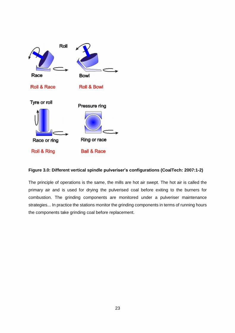
The different vertical spindle coal pulveriser’s configurations are shown below
23
Figure 3.0: Different vertical spindle pulveriser’s configurations (CoalTech: 2007:1-2)
The principle of operations is the same, the mills are hot air swept. The hot air is called the
primary air and is used for drying the pulverised coal before exiting to the burners for
combustion. The grinding components are monitored under a pulveriser maintenance
strategies... In practice the stations monitor the grinding components in terms of running hours
the components take grinding coal before replacement.
24
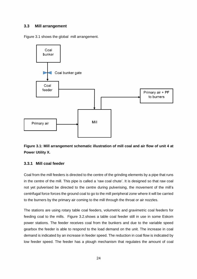
3.3 Mill arrangement
Figure 3.1 shows the global mill arrangement.
Figure 3.1: Mill arrangement schematic illustration of mill coal and air flow of unit 4 at
Power Utility X.
3.3.1 Mill coal feeder
Coal from the mill feeders is directed to the centre of the grinding elements by a pipe that runs
in the centre of the mill. This pipe is called a ‘raw coal chute’. It is designed so that raw coal
not yet pulverised be directed to the centre during pulverising, the movement of the mill’s
centrifugal force forces the ground coal to go to the mill peripheral zone where it will be carried
to the burners by the primary air coming to the mill through the throat or air nozzles.
The stations are using rotary table coal feeders, volumetric and gravimetric coal feeders for
feeding coal to the mills. Figure 3.2.shows a table coal feeder still in use in some Eskom
power stations. The feeder receives coal from the bunkers and due to the variable speed
gearbox the feeder is able to respond to the load demand on the unit. The increase in coal
demand is indicated by an increase in feeder speed. The reduction in coal flow is indicated by
low feeder speed. The feeder has a plough mechanism that regulates the amount of coal
25
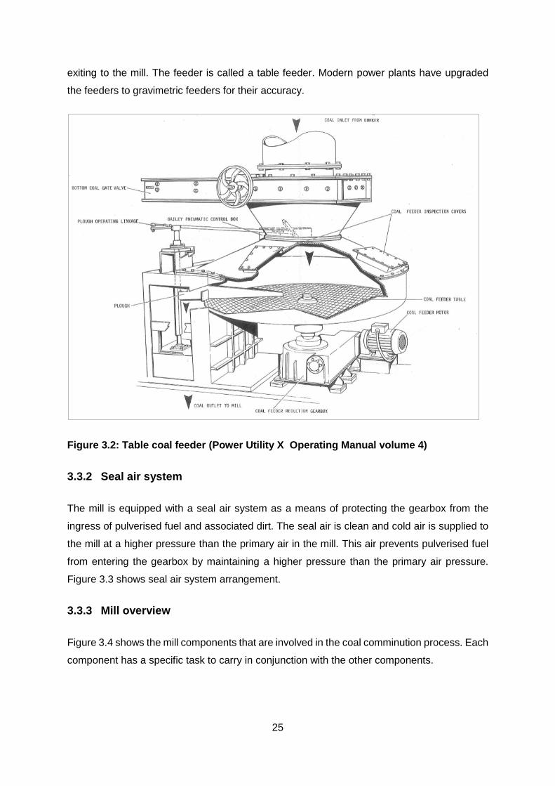
exiting to the mill. The feeder is called a table feeder. Modern power plants have upgraded
the feeders to gravimetric feeders for their accuracy.
Figure 3.2: Table coal feeder (Power Utility X Operating Manual volume 4)
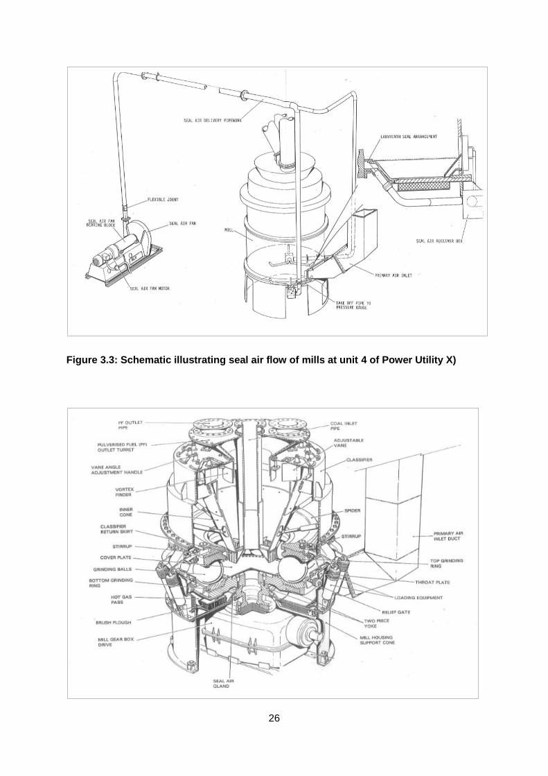
3.3.2 Seal air system
The mill is equipped with a seal air system as a means of protecting the gearbox from the
ingress of pulverised fuel and associated dirt. The seal air is clean and cold air is supplied to
the mill at a higher pressure than the primary air in the mill. This air prevents pulverised fuel
from entering the gearbox by maintaining a higher pressure than the primary air pressure.
Figure 3.3 shows seal air system arrangement.
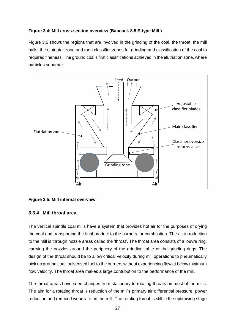
3.3.3 Mill overview
Figure 3.4 shows the mill components that are involved in the coal comminution process. Each
component has a specific task to carry in conjunction with the other components.
26
Figure 3.3: Schematic illustrating seal air flow of mills at unit 4 of Power Utility X)
27
Figure 3.4: Mill cross-section overview (Babcock 8.5 E-type Mill )
Figure 3.5 shows the regions that are involved in the grinding of the coal, the throat, the mill
balls, the elutriator zone and then classifier zones for grinding and classification of the coal to
required fineness. The ground coal’s first classifications achieved in the elutriation zone, where
particles separate.
Figure 3.5: Mill internal overview
3.3.4 Mill throat area
The vertical spindle coal mills have a system that provides hot air for the purposes of drying
the coal and transporting the final product to the burners for combustion. The air introduction
to the mill is through nozzle areas called the ‘throat’. The throat area consists of a louvre ring,
carrying the nozzles around the periphery of the grinding table or the grinding rings. The
design of the throat should be to allow critical velocity during mill operations to pneumatically
pick up ground coal, pulverised fuel to the burners without experiencing flow at below minimum
flow velocity. The throat area makes a large contribution to the performance of the mill.
The throat areas have seen changes from stationary to rotating throats on most of the mills.
The aim for a rotating throat is reduction of the mill’s primary air differential pressure, power
reduction and reduced wear rate on the mill. The rotating throat is still in the optimising stage
Air Air
Grinding zone
Main classifier
OutputFeed
Adjustable classifier blades
Elutriation zone
Classifier oversize returns valve
28
and there are experiments being done to optimise the use of rotating throats and evaluation
of benefits in terms of mill operating costs. The throat velocities were measured by pulverised
fuel sampling and determining the velocities in the pipes and calculating fuel quantities in each
pipe.
3.3.5 Primary air system
The primary air system provides the drying hot air to the coal being pulverised on the mill-
grinding elements. This air is supplied from the air pre-heating system of the boiler. As the
combustion air is supplied to the boiler, it is pre-heated in the air heaters and then split into
two streams. The stream of the air termed ‘primary air’ goes to the milling plant as part of air
that helps with the drying of the coal and, on its way to the burners, carries in suspension
pulverised fuel to the burners. The velocity of flow is provided by the throat area around the
mill. The other part, the secondary air, is directed to the furnace and helps in the combustion
of pulverised fuel exiting at the burners. The velocity traverses the primary air duct and
provides information to calculate velocity and air-flow mass flow rates (Gill,1984:234-239,
(Vijiapurapu et al., 2006:854-866; Shi & He, 2013) .
3.3.6 Grinding elements
The grinding elements of the vertical spindle coal mills depend on the type of mill. The Babcock
E-type mill has grinding balls in between two rings forming a ball-bearing like structure for coal
grinding. The upper ring is stationary while the bottom ring is moving as it is coupled to the
gearbox input shaft. The loading pressure is exerted on the upper ring during grinding. The
grinding elements are of high-wear resistance material and the wear rate is comparable to the
hours the mill would have operated. The roller and table/roller and bowl have rollers that have
metal tyres to grind the coal. The tyres are also made of high-wear resistant material and
replacements are due to measurements and wear monitoring programs. The rollers are also
incorporated with the hydraulic pressure-exerting system that makes sure pressure is applied
to the grinding rollers for effective grinding and fineness.
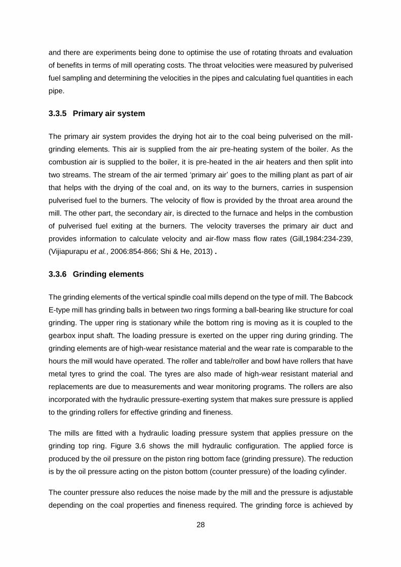
The mills are fitted with a hydraulic loading pressure system that applies pressure on the
grinding top ring. Figure 3.6 shows the mill hydraulic configuration. The applied force is
produced by the oil pressure on the piston ring bottom face (grinding pressure). The reduction
is by the oil pressure acting on the piston bottom (counter pressure) of the loading cylinder.
The counter pressure also reduces the noise made by the mill and the pressure is adjustable
depending on the coal properties and fineness required. The grinding force is achieved by
29
adjustment of the pressure in accordance with the feeder speed whilst the control valves adjust
the pressure.
Figure 3.6: Hydraulic cylinder configuration (Lin and Penterson, 2004:6)
3.3.7 Mill pyrites rejecting system
The primary air through the nozzle system transports the fine pulverised fuel to the burners
for combustion to take place. The heavier particles are returned to the grinding zone for further
reductions in size. The materials that cannot be lifted by the primary air fall into the throat area
and are directed to the reject boxes.
3.4 Mill configuration
The design of the boiler is for the mills to supply the required heat by supplying the amount of
coal required. The boiler running under design coal is manageable within the coal envelope.
Most power stations are running with coal that was taken account of in the design. It was
explained in Chapter 1 in the problem statement, that coal has found better paying customers.
The stations have to use the available coal and this is blended to make a mixture similar to
the design coal. The configuration of mills is that they supply specific burners to give the heat
required.
30
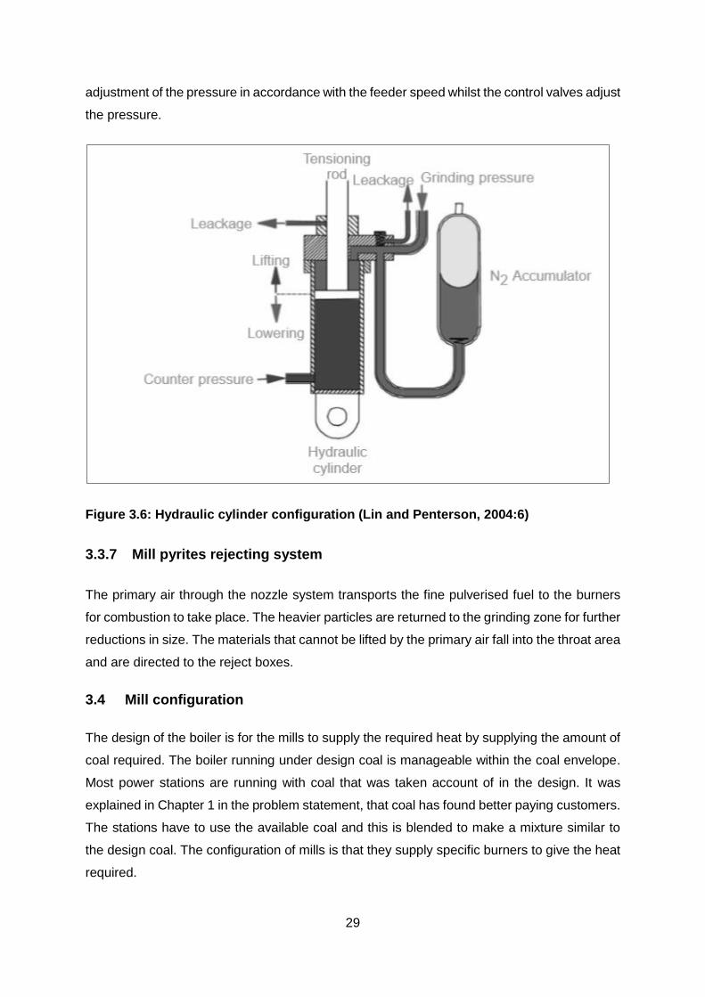
According to Arauzo and Cortés (1995:397-397) mill configuration is represented through the
Average Burner Height (ABH) which is evaluated as follows:
𝑨𝑩𝑯 = ∑ 𝒓𝒑𝒎𝒊𝑯𝒊
∑ 𝒓𝒑𝒎𝒊 3.1
where: i = mill’s in service, 𝑟𝑝𝑚𝑖 = the angular velocity of the volumetric feeder of each mill
coal flow of mill I and 𝐻𝑖 = the burner plane height associated with each mill.
The power station has the mills categorised as top, middle and bottom mills. Table 3.1 shows
the mill configuration. The bottom mills and the middle mills are in service during boiler
operation. One top mill is selected to maintain the steam temperatures. The mills are run with
the heat requirement for the load. The load on a unit requires five mills in service out of the six
mills available on a unit. Each level of the boiler heat design is allocated burners that are
associated with that level and supplied coal by the mills associated with the levels.
Table 3.1: Mills configuration of Power Utility X unit 4
Top mills C F
Middle mills B D
Bottom mills A E
Average burner height (m) Mills in service Burners supplied by mills
14.85 A A1,A2,A3,A4
14.85 B B1,B2,B3,B4
14.85 C C1,C2,C3,C4
17.44 D D1,D2,D3,D4
12.19 E E1,E2,E3,E4
17.44 F F1,F2,F3,F4

31
The top, middle and bottom positions are average burner heights associated with the mills.
3.5 Conclusion
The purpose of this chapter was to give an overview of the design features of vertical spindle
coal pulverisers and the functionality of the associated mill components.The Babcock 8.5 E-
type mill configuration on Unit Four was presented in this chapter. The next chapter presents
the methodology of testing the mill and performance evaluation.
32
4 Simulation of the vertical spindle coal pulverisers effectiveness
4.1 Introduction
The aim of this research project is to investigate the effect of coal feedstock property variation
on the vertical spindle coal pulverising mill performance to facilitate optimal plant performance.
This chapter focuses on the methods of the test to be carried out in evaluating the performance
and optimisation of vertical spindle coal pulverisers.
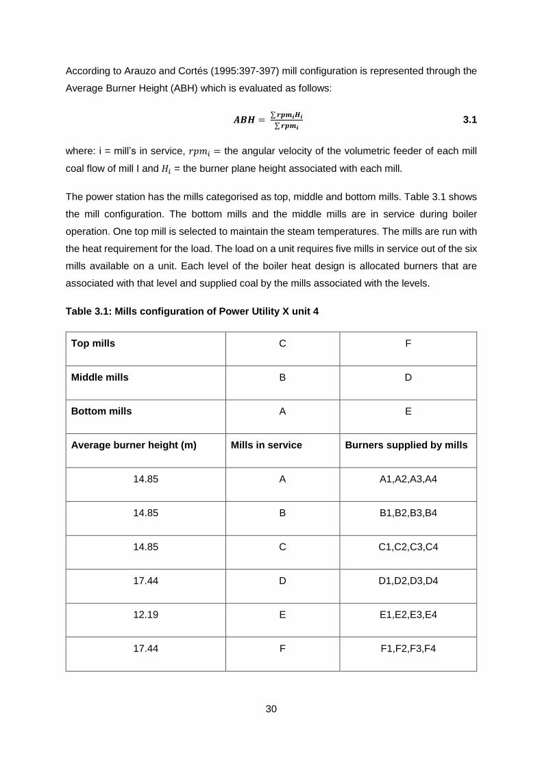
4.2 Research methodology overview
Figure 4.1: Research methodology overview
4.3 Plant design data analysis
In order to understand the performance of the mills at present, the design data is analysed to
check any changes that have been implemented since acceptance time. The data analysis is
performed on the following:
design data of the mills, the mills are 8.5 Babcock E-type mills and vertical spindle;
acceptance test data from the acceptance tests that were carried out by Babcock
when the mills were handed over to Eskom after installation. The acceptance test of
mills give detail on mill performance, pulverised fuel fineness and pulverised fuel
distribution achieved during the test;
acceptance test proves the design and these values are used when assessing the mill
performance;
33
the boiler design data is analysed to assess the energy requirement that the mills
supply to the boiler to generate steam;
rating of the mills in tonnes/hr; and
coal analysis and properties that were considered in rating the mills.
4.4 Plant tests
4.4.1 PF sampling
The mill performance is evaluated by use of the acceptance test data as the baseline and by
using the current operating data. The mill test is carried out to collect data that is analysed to
discover potential areas of improvement .Present data gives the operation of the mill. Plant
tests that assess the performance of the mill are:
pulverised fuel sampling in the pipes leading to the burners;
pulverised fuel pipes are traversed during sampling to measure velocity pressure,
static pressure and temperature of pulverised air mixture;
all the associated activities in conducting pulverised fuel sampling is to use the test
data to determine;
coal flow through the mill;
air flow through the mill;
particle carrying velocities;
pulverised fuel mass flow and distribution;
mill performance evaluation; and
pulverised fuel fineness.
4.4.2 Mill load simulations
Simulation of mill loads using air flows is done to check the mill output. A comparison between
control room mill load readings, simulated mill load and sampled mill load is carried out.
4.4.3 Hardgrove Grindability index
Using the method developed by Hardgrove the Hardgrove Grindability Index is determined.
The HGI serves as a means for estimating how various coals behave in commercial
pulverisers. The mill rated output is based on the Hardgrove grindability index. Grootvlei Power
Station is supplied with coal from more than 12 mines. The mines blend the coal to meet the
34
ash content and the calorific values of the coal. The HGI is evaluated to determine the current
mill output with the new coal supply. Refer to table 6.3 for the HGI results.
4.4.4 Abrasive Index
The coal hardness causes wear as the mill operates. Wear affects the life of mill components
and pulverised fuel pipes. The understanding of the wear induced by the coal is evaluated by
an index called the ‘Abrasive Index’. This index is defined as the material’s ability to remove
material from the grinding surface. A sample of coal is used to determine the Abrasive Index.
Four metal blades of known weight are fixed on the Abrasive Index testing machine and run
through the coal for specified times and revolutions. The loss in mass of the four blades is
used to determine the Abrasive Index. The Abrasive Index is evaluated to determine the wear
rate on mill grinding components from the new coal the station is using. Refer to table 6.1 for
the abrasive Index results.
4.4.5 Excel spreadsheet for mill performance evaluation
An Excel spreadsheet is formulated using Equations 2.22 to 2.25. The spreadsheet input
parameters are: coal flow, primary air flow, primary air temperature, mill grinding pressure and
mill dimensions.
The mill outputs of the spreadsheet are: mill frictional factor, mill power consumption, cut of
velocity of pulverised fuel and cut of diameter of pulverised fuel. The spreadsheet is used to
evaluate the effect of varying operating parameters on the mill during operation.
4.4.6 Heat balance
A heat balance spreadsheet is used to evaluate the heat into the mill used for drying the coal.
Heat out of the mill is determined by calculating the heat out. The energy available is evaluated
to determine the drying constraint of the mill. The heat balance spreadsheet is based on
Equations 2.10 to 2.21.
4.4.7 Conclusion
This chapter focused on the methods of the test to be carried out in evaluating the performance
and optimisation of vertical spindle coal pulverisers. An overview on plant tests which include
PF sampling, mill load simulation, Hardgrove Grindability Index, Abrasive Index and an Excel
spreadsheet for mill performance evaluation and heat balance was presented.

35
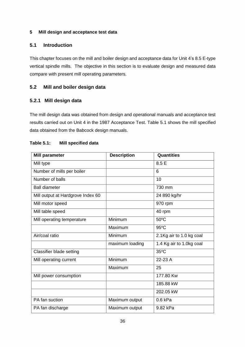
36
5 Mill design and acceptance test data
5.1 Introduction
This chapter focuses on the mill and boiler design and acceptance data for Unit 4’s 8.5 E-type
vertical spindle mills. The objective in this section is to evaluate design and measured data
compare with present mill operating parameters.
5.2 Mill and boiler design data
5.2.1 Mill design data
The mill design data was obtained from design and operational manuals and acceptance test
results carried out on Unit 4 in the 1987 Acceptance Test. Table 5.1 shows the mill specified
data obtained from the Babcock design manuals.
Table 5.1: Mill specified data
Mill parameter Description Quantities
Mill type 8.5 E
Number of mills per boiler 6
Number of balls 10
Ball diameter 730 mm
Mill output at Hardgrove Index 60 24 890 kg/hr
Mill motor speed 970 rpm
Mill table speed 40 rpm
Mill operating temperature Minimum 50oC
Maximum 95oC
Air/coal ratio Minimum 2.1Kg air to 1.0 kg coal
maximum loading 1.4 Kg air to 1.0kg coal
Classifier blade setting 35oC
Mill operating current Minimum 22-23 A
Maximum 25
Mill power consumption 177.80 Kw
185.88 kW
202.05 kW
PA fan suction Maximum output 0.6 kPa
PA fan discharge Maximum output 9.82 kPa
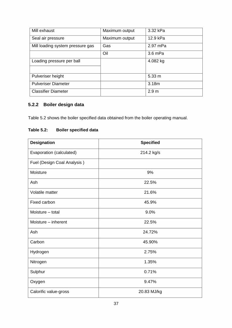
37
Mill exhaust Maximum output 3.32 kPa
Seal air pressure Maximum output 12.9 kPa
Mill loading system pressure gas Gas 2.97 mPa
Oil 3.6 mPa
Loading pressure per ball 4.082 kg
Pulveriser height 5.33 m
Pulveriser Diameter 3.18m
Classifier Diameter 2.9 m
5.2.2 Boiler design data
Table 5.2 shows the boiler specified data obtained from the boiler operating manual.
Table 5.2: Boiler specified data
Designation Specified
Evaporation (calculated) 214.2 kg/s
Fuel (Design Coal Analysis )
Moisture 9%
Ash 22.5%
Volatile matter 21.6%
Fixed carbon 45.9%
Moisture – total 9.0%
Moisture – inherent 22.5%
Ash 24.72%
Carbon 45.90%
Hydrogen 2.75%
Nitrogen 1.35%
Sulphur 0.71%
Oxygen 9.47%
Calorific value-gross 20.83 MJ/kg
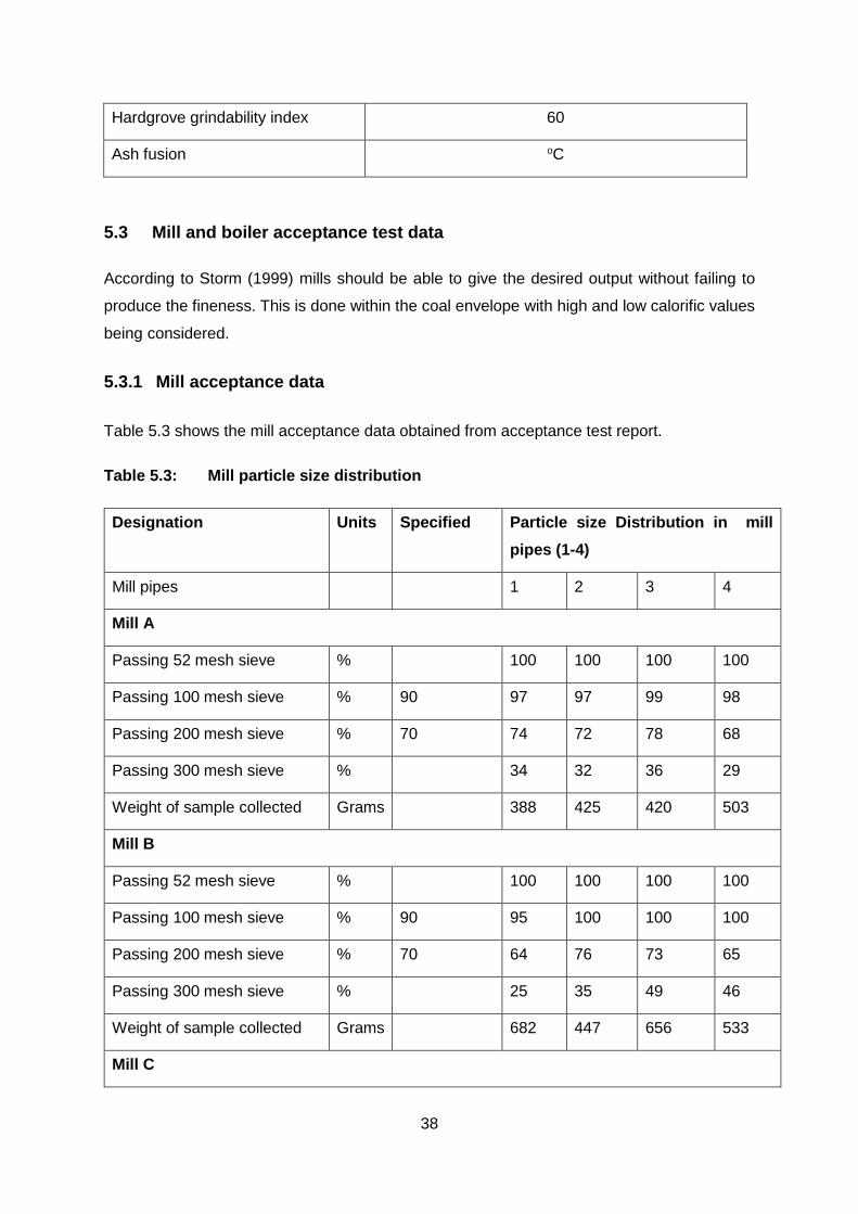
38
Hardgrove grindability index 60
Ash fusion oC
5.3 Mill and boiler acceptance test data
According to Storm (1999) mills should be able to give the desired output without failing to
produce the fineness. This is done within the coal envelope with high and low calorific values
being considered.
5.3.1 Mill acceptance data
Table 5.3 shows the mill acceptance data obtained from acceptance test report.
Table 5.3: Mill particle size distribution
Designation Units Specified Particle size Distribution in mill
pipes (1-4)
Mill pipes 1 2 3 4
Mill A
Passing 52 mesh sieve % 100 100 100 100
Passing 100 mesh sieve % 90 97 97 99 98
Passing 200 mesh sieve % 70 74 72 78 68
Passing 300 mesh sieve % 34 32 36 29
Weight of sample collected Grams 388 425 420 503
Mill B
Passing 52 mesh sieve % 100 100 100 100
Passing 100 mesh sieve % 90 95 100 100 100
Passing 200 mesh sieve % 70 64 76 73 65
Passing 300 mesh sieve % 25 35 49 46
Weight of sample collected Grams 682 447 656 533
Mill C
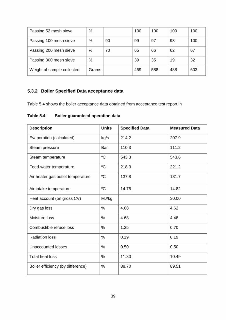
39
Passing 52 mesh sieve % 100 100 100 100
Passing 100 mesh sieve % 90 99 97 98 100
Passing 200 mesh sieve % 70 65 66 62 67
Passing 300 mesh sieve % 39 35 19 32
Weight of sample collected Grams 459 588 488 603
5.3.2 Boiler Specified Data acceptance data
Table 5.4 shows the boiler acceptance data obtained from acceptance test report.in
Table 5.4: Boiler guaranteed operation data
Description Units Specified Data Measured Data
Evaporation (calculated) kg/s 214.2 207.9
Steam pressure Bar 110.3 111.2
Steam temperature oC 543.3 543.6
Feed-water temperature oC 218.3 221.2
Air heater gas outlet temperature oC 137.8 131.7
Air intake temperature oC 14.75 14.82
Heat account (on gross CV) MJ/kg 30.00
Dry gas loss % 4.68 4.62
Moisture loss % 4.68 4.48
Combustible refuse loss % 1.25 0.70
Radiation loss % 0.19 0.19
Unaccounted losses % 0.50 0.50
Total heat loss % 11.30 10.49
Boiler efficiency (by difference) % 88.70 89.51
40
5.4 Discussion
Table 5.3 shows the mill acceptance data obtained from the acceptance test data manual.
The mill grindability index was analysed for the acceptance tests and these are summarised
in the Table 5.3.
The 75 µm sieve is critical in the mill acceptance pulverised coal fineness data analysis. The
fineness for Mill A, Mill D and Mill E were above the design of 70% coal fineness. Mill B was
on par and the lowest fineness was on Mill C that registered 65% through the 75µm sieve.
The pulverised fuel distribution measured during the acceptance test show that the unit mass
was equally distributed to the burners. The Mill F was not available during the acceptance
tests, and the performance is considered to be of the same standard as achieved by the five
mills.
The design was based on the coal from a dedicated coal mine which was closed when Power
Utility X was mothballed. During the acceptance test the coal analysis was at 62 Hardgrove
Grindability Index. The coal was soft as indicated by the HGI value in table 5.2.
Mill A’s design pulverised coal fineness is 70% through the 75µm sieve. During the acceptance
test the pulverised coal fineness measured on all four 4A mill pipes as:
pipe 1 fineness of pulverised fuel was 74% through the 75 µm sieve;
pipe 2 fineness of pulverised fuel was 72% through the 75µm sieve;
pipe 3 fineness of pulverised fuel was 78% through the 75µm sieve;
pipe 4 fineness of pulverised fuel was 68% through the 75µm sieve; and
average pulverised fuel fineness of the four pipes was 74% through the 75µm sieve.
The coal moisture was 9.1%, this is the mill drying capacity constraint. The boilers have been
retrofitted with low NOx burners replacing the axial flow burners that were originally installed
on all units, including Unit 4 at the Power Utility X. The classifier vanes’ setting was angled at
a 35-degree opening during the acceptance test of the mill. Currently the mill classifier blades’
setting is at a 40-degree angle opening.
The acceptance test data show that the mills achieved the design output and fineness above
70% through the 75µm sieve. The pulverised fuel was equally distributed in the pipes to the
burners. The coal had an HGI of 62, which was above the 60 design. This means the coal
pulverised was softer than the design coal. Mill output was achieved using the softer coal.

41
Unit 4 at Power Utility X is retrofitted with low NOx burners replacing the Babcock axial flow
burners. The impact of the low NOx burners on the performance of the mill be considered. The
mill classifier blades’ setting is 40-degrees, giving a 5-degree opening of the classifier vanes
from the 35-degree design and acceptance test setting.
5.5 Conclusion
The mill and boiler design and acceptance test data were analysed in this chapter.
42
6 Plant tests
6.1 Introduction
The aim of this chapter is to present the Plant Test performed to evaluate the mill performance.
The tests covered in this chapter include Abrasive Index, Hardgrove Grindability Index, PF
sampling and the power consumption tests. The tests were conducted at an Eskom Power
Utility X Unit 4 Mills A-F.
6.2 Abrasive Index
The Abrasive Index is measured by using an abrasion testing machine. Four metal blades
made from carbon steel with a hardness of 160/-15 Vickers and dimensions of 38 X 38 X 11
mm (+- 0.1mm). The index is defined as an index that shows the abrasion properties of coal
on the equipment used to grind the coal before the coal is used as fuel in the boilers. Coal
users like to have abrasion index less than 200, greater than 200 users prefer to pay less for
this type of coal.
The test of the abrasion index is measured using the equipment called Abrasion Test
Apparatus. The station carries out this test at the station laboratory. The equipment has four
blades knives which are made from carbon steel with a hardness of 160/-15 Vickers and the
dimensions of 38x38x11 mm (+-0.1 mm).
The test will be spinning the blades in coal sample being tested with a speed of 1470/- 30
rounds /min, 1200/-20 rounds /min. The sample size used is 10 kg with a top size greater than
16mm.
The samples are milled to obtain particle size 6.7mm and test is carried out on samples of the
milling results with a weight 0f 2/-0.1 kg for each test. The loss in weight of the blades is used
to calculate the abrasion Index (BS, 1016: Part 19).
6.2.1 Abrasive Index test procedure
The testing machine blade weights are measured before they are spun, stirring coal samples
are tested with a speed of 1470 rpm for 30 minutes. After the 30 minutes the blade weights
are measured. The index unit is milligrams of metal blades that erode per kilogram of coal
sample used.
The blades’ mass loss is calculated by subtracting the mass of the blades after (Bi) the test
from the mass of the blades before (A1i), where subscript I is the blade number.
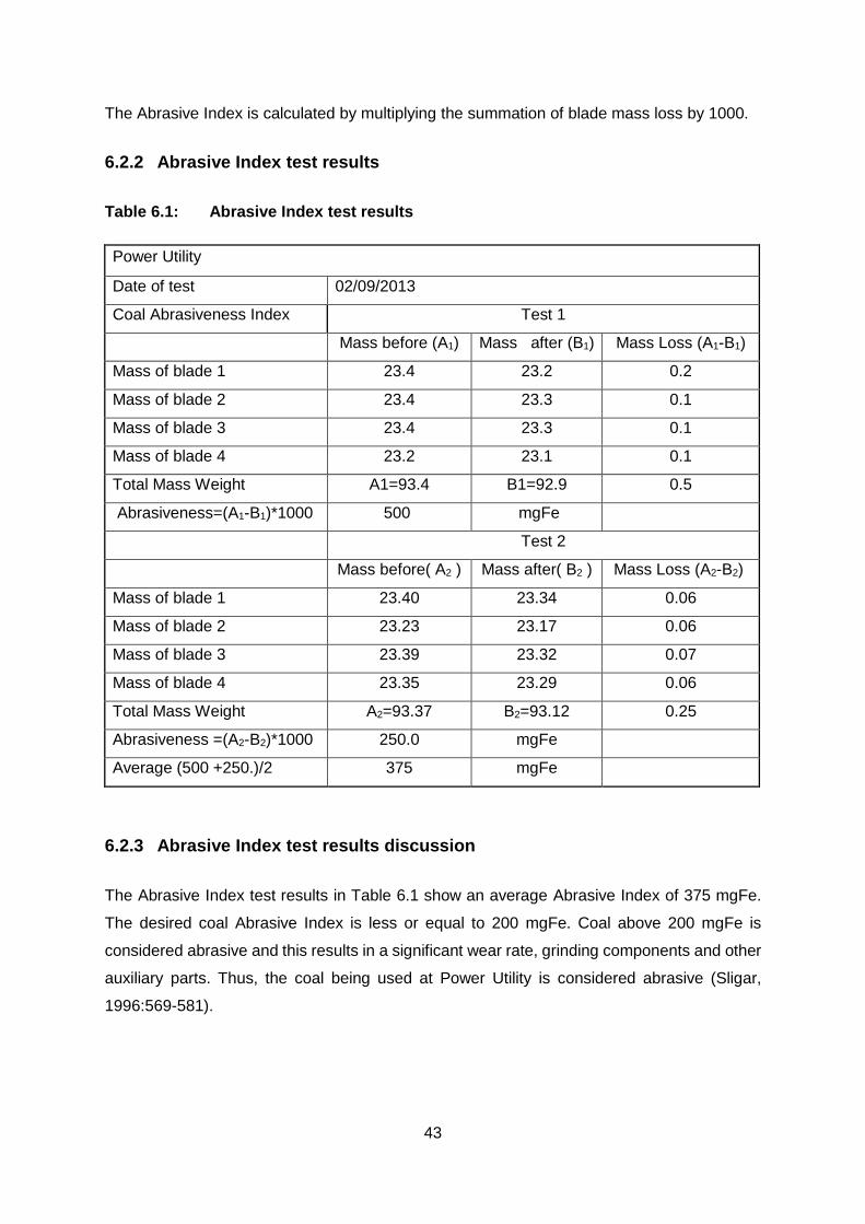
43
The Abrasive Index is calculated by multiplying the summation of blade mass loss by 1000.
6.2.2 Abrasive Index test results
Table 6.1: Abrasive Index test results
Power Utility
Date of test 02/09/2013
Coal Abrasiveness Index Test 1
Mass before (A1) Mass after (B1) Mass Loss (A1-B1)
Mass of blade 1 23.4 23.2 0.2
Mass of blade 2 23.4 23.3 0.1
Mass of blade 3 23.4 23.3 0.1
Mass of blade 4 23.2 23.1 0.1
Total Mass Weight A1=93.4 B1=92.9 0.5
Abrasiveness=(A1-B1)*1000 500 mgFe
Test 2
Mass before( A2 ) Mass after( B2 ) Mass Loss (A2-B2)
Mass of blade 1 23.40 23.34 0.06
Mass of blade 2 23.23 23.17 0.06
Mass of blade 3 23.39 23.32 0.07
Mass of blade 4 23.35 23.29 0.06
Total Mass Weight A2=93.37 B2=93.12 0.25
Abrasiveness =(A2-B2)*1000 250.0 mgFe
Average (500 +250.)/2 375 mgFe
6.2.3 Abrasive Index test results discussion
The Abrasive Index test results in Table 6.1 show an average Abrasive Index of 375 mgFe.
The desired coal Abrasive Index is less or equal to 200 mgFe. Coal above 200 mgFe is
considered abrasive and this results in a significant wear rate, grinding components and other
auxiliary parts. Thus, the coal being used at Power Utility is considered abrasive (Sligar,
1996:569-581).
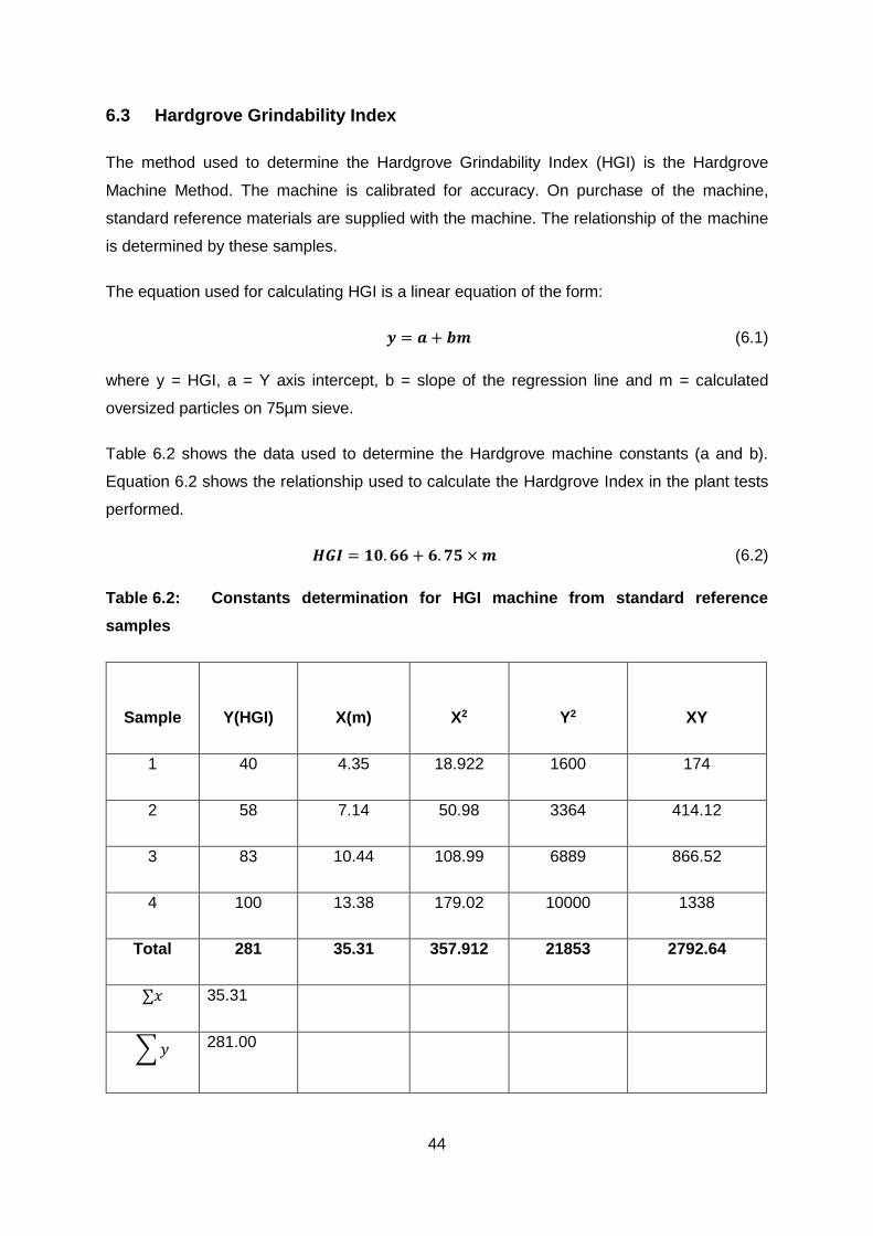
44
6.3 Hardgrove Grindability Index
The method used to determine the Hardgrove Grindability Index (HGI) is the Hardgrove
Machine Method. The machine is calibrated for accuracy. On purchase of the machine,
standard reference materials are supplied with the machine. The relationship of the machine
is determined by these samples.
The equation used for calculating HGI is a linear equation of the form:
𝒚 = 𝒂 + 𝒃𝒎 (6.1)
where y = HGI, a = Y axis intercept, b = slope of the regression line and m = calculated
oversized particles on 75µm sieve.
Table 6.2 shows the data used to determine the Hardgrove machine constants (a and b).
Equation 6.2 shows the relationship used to calculate the Hardgrove Index in the plant tests
performed.
𝑯𝑮𝑰 = 𝟏𝟎. 𝟔𝟔 + 𝟔. 𝟕𝟓 × 𝒎 (6.2)
Table 6.2: Constants determination for HGI machine from standard reference
samples
Sample
Y(HGI)
X(m)
X2
Y2
XY
1 40 4.35 18.922 1600 174
2 58 7.14 50.98 3364 414.12
3 83 10.44 108.99 6889 866.52
4 100 13.38 179.02 10000 1338
Total 281 35.31 357.912 21853 2792.64
∑𝑥 35.31
∑ 𝑦 281.00
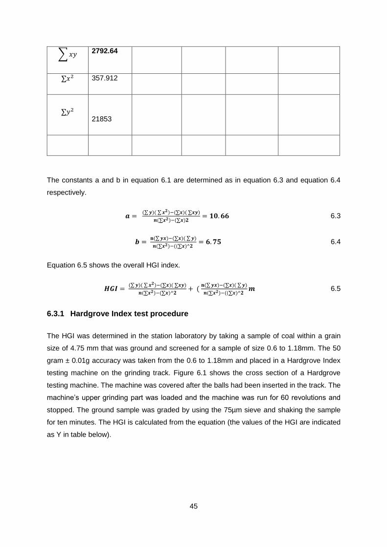
45
∑ 𝑥𝑦 2792.64
∑𝑥2 357.912
∑𝑦2
21853
The constants a and b in equation 6.1 are determined as in equation 6.3 and equation 6.4
respectively.
𝒂 = (∑ 𝒚)( ∑ 𝒙𝟐)−(∑𝒙)( ∑𝒙𝒚)
𝒏(∑𝒙𝟐)−(∑𝒙)𝟐= 𝟏𝟎. 𝟔𝟔 6.3
𝒃 = 𝐧(∑ 𝒚𝒙)−(∑𝒙)( ∑ 𝒚)
𝒏(∑𝒙𝟐)−((∑𝒙)^𝟐 = 𝟔. 𝟕𝟓 6.4
Equation 6.5 shows the overall HGI index.
𝑯𝑮𝑰 = (∑ 𝒚)( ∑ 𝒙𝟐)−(∑𝒙)( ∑𝒙𝒚)
𝒏(∑𝒙𝟐)−(∑𝒙)^𝟐+ (
𝐧(∑ 𝒚𝒙)−(∑𝒙)( ∑ 𝒚)
𝒏(∑𝒙𝟐)−((∑𝒙)^𝟐 𝒎 6.5
6.3.1 Hardgrove Index test procedure
The HGI was determined in the station laboratory by taking a sample of coal within a grain
size of 4.75 mm that was ground and screened for a sample of size 0.6 to 1.18mm. The 50
gram ± 0.01g accuracy was taken from the 0.6 to 1.18mm and placed in a Hardgrove Index
testing machine on the grinding track. Figure 6.1 shows the cross section of a Hardgrove
testing machine. The machine was covered after the balls had been inserted in the track. The
machine’s upper grinding part was loaded and the machine was run for 60 revolutions and
stopped. The ground sample was graded by using the 75µm sieve and shaking the sample
for ten minutes. The HGI is calculated from the equation (the values of the HGI are indicated
as Y in table below).
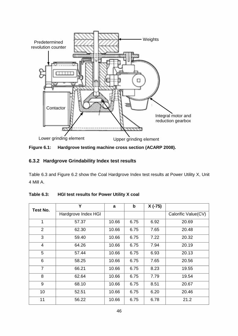
46
Figure 6.1: Hardgrove testing machine cross section (ACARP 2008).
6.3.2 Hardgrove Grindability Index test results
Table 6.3 and Figure 6.2 show the Coal Hardgrove Index test results at Power Utility X, Unit
4 Mill A.
Table 6.3: HGI test results for Power Utility X coal
Test No. Y a b X (-75)
Hardgrove Index HGI Calorific Value(CV)
1 57.37 10.66 6.75 6.92 20.69
2 62.30 10.66 6.75 7.65 20.48
3 59.40 10.66 6.75 7.22 20.32
4 64.26 10.66 6.75 7.94 20.19
5 57.44 10.66 6.75 6.93 20.13
6 58.25 10.66 6.75 7.65 20.56
7 66.21 10.66 6.75 8.23 19.55
8 62.64 10.66 6.75 7.79 19.54
9 68.10 10.66 6.75 8.51 20.67
10 52.51 10.66 6.75 6.20 20.46
11 56.22 10.66 6.75 6.78 21.2
Integral motor and reduction gearbox
Weights Predetermined
revolution counter
Contactor
Lower grinding element Upper grinding element
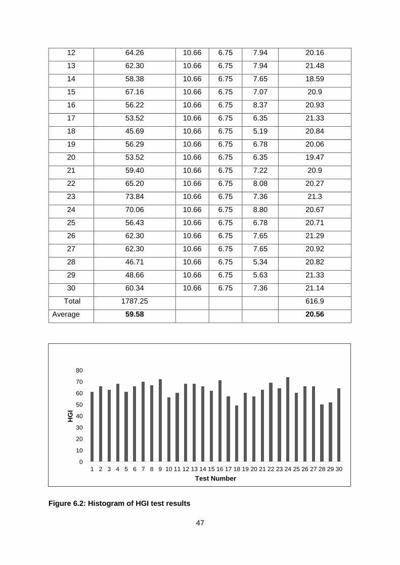
47
12 64.26 10.66 6.75 7.94 20.16
13 62.30 10.66 6.75 7.94 21.48
14 58.38 10.66 6.75 7.65 18.59
15 67.16 10.66 6.75 7.07 20.9
16 56.22 10.66 6.75 8.37 20.93
17 53.52 10.66 6.75 6.35 21.33
18 45.69 10.66 6.75 5.19 20.84
19 56.29 10.66 6.75 6.78 20.06
20 53.52 10.66 6.75 6.35 19.47
21 59.40 10.66 6.75 7.22 20.9
22 65.20 10.66 6.75 8.08 20.27
23 73.84 10.66 6.75 7.36 21.3
24 70.06 10.66 6.75 8.80 20.67
25 56.43 10.66 6.75 6.78 20.71
26 62.30 10.66 6.75 7.65 21.29
27 62.30 10.66 6.75 7.65 20.92
28 46.71 10.66 6.75 5.34 20.82
29 48.66 10.66 6.75 5.63 21.33
30 60.34 10.66 6.75 7.36 21.14
Total 1787.25 616.9
Average 59.58 20.56
Figure 6.2: Histogram of HGI test results
0
10
20
30
40
50
60
70
80
1 2 3 4 5 6 7 8 9 10 11 12 13 14 15 16 17 18 19 20 21 22 23 24 25 26 27 28 29 30
HG
I
Test Number
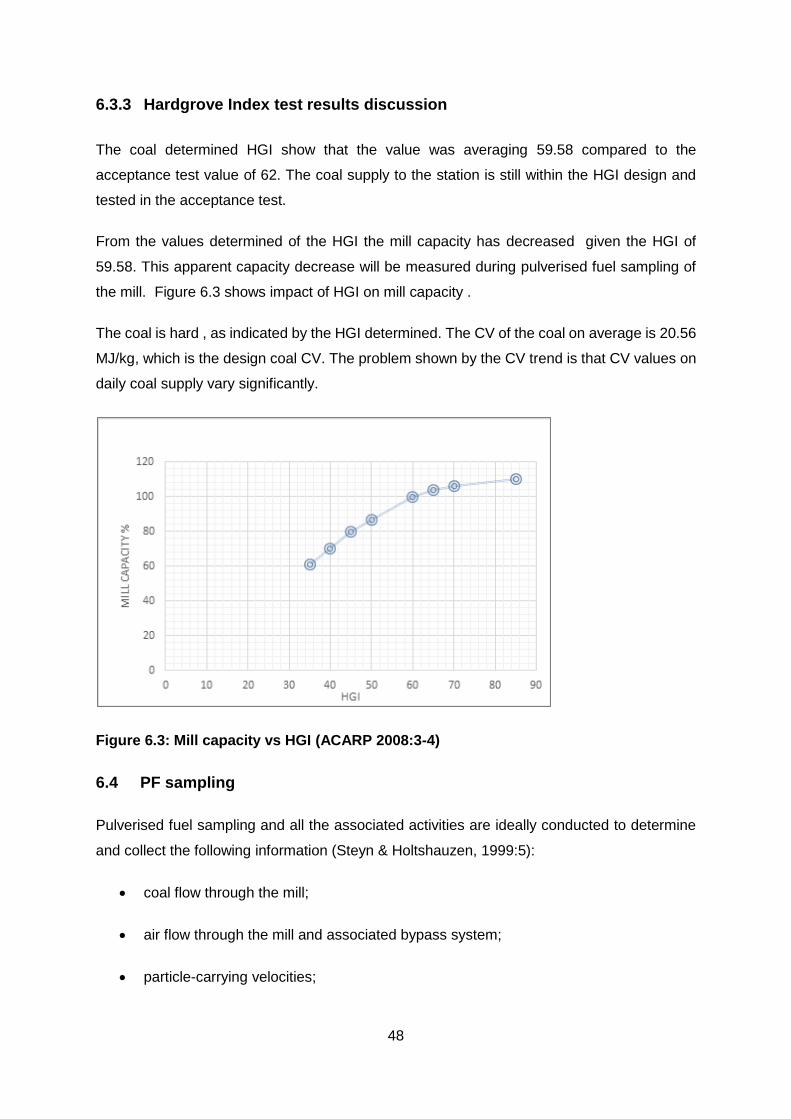
48
6.3.3 Hardgrove Index test results discussion
The coal determined HGI show that the value was averaging 59.58 compared to the
acceptance test value of 62. The coal supply to the station is still within the HGI design and
tested in the acceptance test.
From the values determined of the HGI the mill capacity has decreased given the HGI of
59.58. This apparent capacity decrease will be measured during pulverised fuel sampling of
the mill. Figure 6.3 shows impact of HGI on mill capacity .
The coal is hard , as indicated by the HGI determined. The CV of the coal on average is 20.56
MJ/kg, which is the design coal CV. The problem shown by the CV trend is that CV values on
daily coal supply vary significantly.
Figure 6.3: Mill capacity vs HGI (ACARP 2008:3-4)
6.4 PF sampling
Pulverised fuel sampling and all the associated activities are ideally conducted to determine
and collect the following information (Steyn & Holtshauzen, 1999:5):
coal flow through the mill;
air flow through the mill and associated bypass system;
particle-carrying velocities;
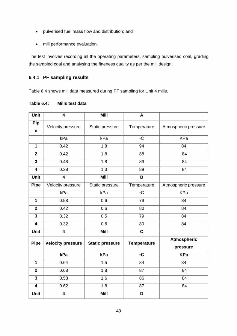
49
pulverised fuel mass flow and distribution; and
mill performance evaluation.
The test involves recording all the operating parameters, sampling pulverised coal, grading
the sampled coal and analysing the fineness quality as per the mill design.
6.4.1 PF sampling results
Table 6.4 shows mill data measured during PF sampling for Unit 4 mills.
Table 6.4: Mills test data
Unit 4 Mill A
Pip
e Velocity pressure Static pressure Temperature Atmospheric pressure
kPa kPa ◦C KPa
1 0.42 1.8 94 84
2 0.42 1.8 88 84
3 0.48 1.8 89 84
4 0.38 1.3 89 84
Unit 4 Mill B
Pipe Velocity pressure Static pressure Temperature Atmospheric pressure
kPa kPa ◦C KPa
1 0.58 0.6 79 84
2 0.42 0.6 80 84
3 0.32 0.5 79 84
4 0.32 0.6 80 84
Unit 4 Mill C
Pipe Velocity pressure Static pressure Temperature Atmospheric
pressure
kPa kPa ◦C KPa
1 0.64 1.5 84 84
2 0.68 1.8 87 84
3 0.58 1.6 86 84
4 0.62 1.8 87 84
Unit 4 Mill D
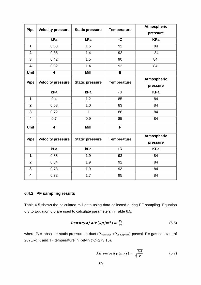
50
Pipe Velocity pressure Static pressure Temperature Atmospheric
pressure
kPa kPa ◦C KPa
1 0.58 1.5 92 84
2 0.38 1.4 92 84
3 0.42 1.5 90 84
4 0.32 1.4 92 84
Unit 4 Mill E
Pipe Velocity pressure Static pressure Temperature Atmospheric
pressure
kPa kPa ◦C KPa
1 0.4 1.2 85 84
2 0.58 1,0 83 84
3 0.72 1 86 84
4 0.7 0.9 85 84
Unit 4 Mill F
Pipe Velocity pressure Static pressure Temperature Atmospheric
pressure
kPa kPa ◦C KPa
1 0.88 1.9 93 84
2 0.84 1.9 92 84
3 0.78 1.9 93 84
4 0.72 1.7 95 84
6.4.2 PF sampling results
Table 6.5 shows the calculated mill data using data collected during PF sampling. Equation
6.3 to Equation 6.5 are used to calculate parameters in Table 6.5.
𝑫𝒆𝒏𝒔𝒊𝒕𝒚 𝒐𝒇 𝒂𝒊𝒓 (𝒌𝒈 𝒎𝟑⁄ ) = 𝑷𝒔
𝑹𝑻 (6.6)
where Ps = absolute static pressure in duct (Pmeasured +Patmosphere) pascal, R= gas constant of
287J/kg.K and T= temperature in Kelvin (oC+273.15).
𝑨𝒊𝒓 𝒗𝒆𝒍𝒐𝒄𝒊𝒕𝒚 (𝒎 𝒔⁄ ) = √𝟐∆𝑷
𝝆 (6.7)
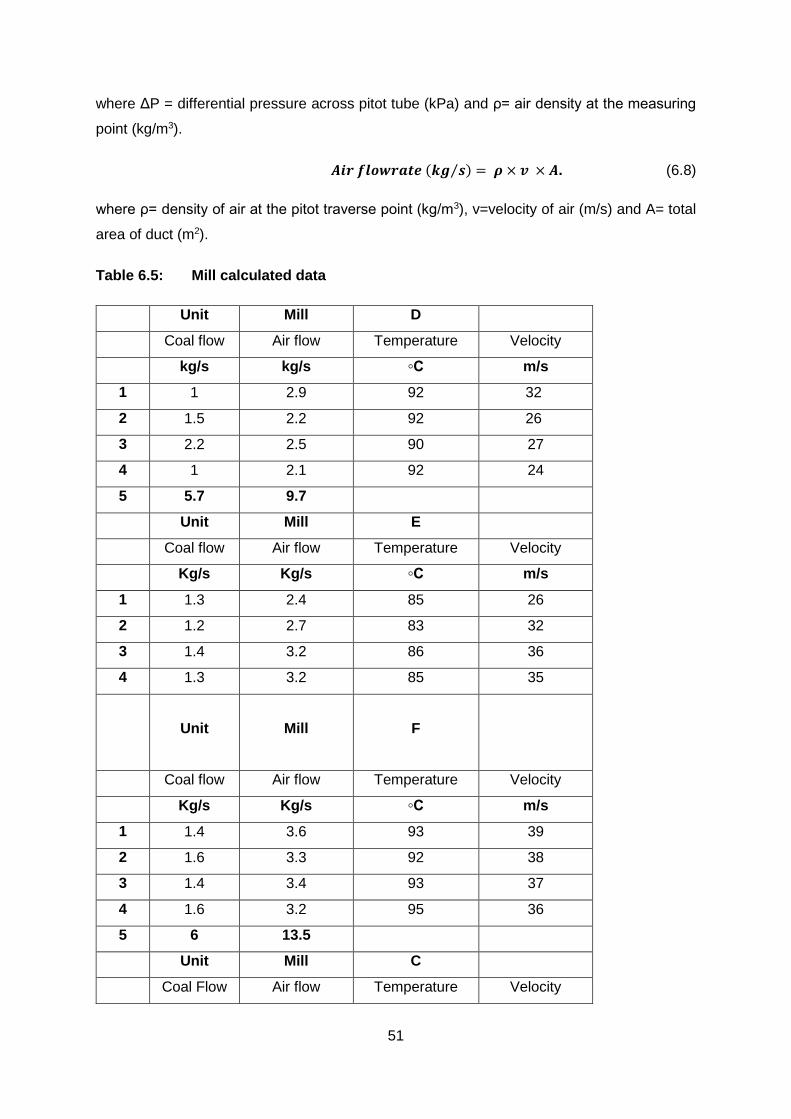
51
where ΔP = differential pressure across pitot tube (kPa) and ρ= air density at the measuring
point (kg/m3).
𝑨𝒊𝒓 𝒇𝒍𝒐𝒘𝒓𝒂𝒕𝒆 (𝒌𝒈 𝒔⁄ ) = 𝝆 × 𝒗 × 𝑨. (6.8)
where ρ= density of air at the pitot traverse point (kg/m3), v=velocity of air (m/s) and A= total
area of duct (m2).
Table 6.5: Mill calculated data
Unit Mill D
Coal flow Air flow Temperature Velocity
kg/s kg/s ◦C m/s
1 1 2.9 92 32
2 1.5 2.2 92 26
3 2.2 2.5 90 27
4 1 2.1 92 24
5 5.7 9.7
Unit Mill E
Coal flow Air flow Temperature Velocity
Kg/s Kg/s ◦C m/s
1 1.3 2.4 85 26
2 1.2 2.7 83 32
3 1.4 3.2 86 36
4 1.3 3.2 85 35
Unit Mill F
Coal flow Air flow Temperature Velocity
Kg/s Kg/s ◦C m/s
1 1.4 3.6 93 39
2 1.6 3.3 92 38
3 1.4 3.4 93 37
4 1.6 3.2 95 36
5 6 13.5
Unit Mill C
Coal Flow Air flow Temperature Velocity
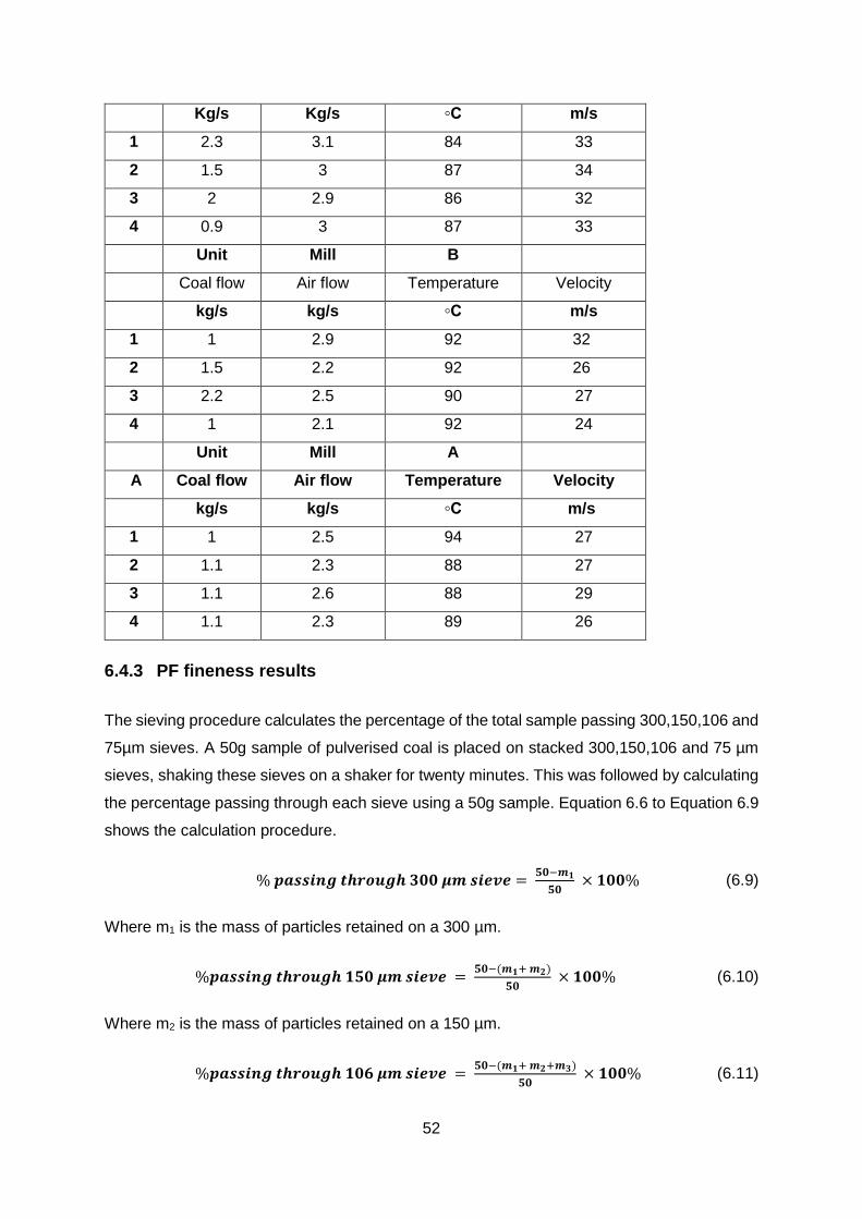
52
Kg/s Kg/s ◦C m/s
1 2.3 3.1 84 33
2 1.5 3 87 34
3 2 2.9 86 32
4 0.9 3 87 33
Unit Mill B
Coal flow Air flow Temperature Velocity
kg/s kg/s ◦C m/s
1 1 2.9 92 32
2 1.5 2.2 92 26
3 2.2 2.5 90 27
4 1 2.1 92 24
Unit Mill A
A Coal flow Air flow Temperature Velocity
kg/s kg/s ◦C m/s
1 1 2.5 94 27
2 1.1 2.3 88 27
3 1.1 2.6 88 29
4 1.1 2.3 89 26
6.4.3 PF fineness results
The sieving procedure calculates the percentage of the total sample passing 300,150,106 and
75µm sieves. A 50g sample of pulverised coal is placed on stacked 300,150,106 and 75 µm
sieves, shaking these sieves on a shaker for twenty minutes. This was followed by calculating
the percentage passing through each sieve using a 50g sample. Equation 6.6 to Equation 6.9
shows the calculation procedure.
% 𝒑𝒂𝒔𝒔𝒊𝒏𝒈 𝒕𝒉𝒓𝒐𝒖𝒈𝒉 𝟑𝟎𝟎 𝝁𝒎 𝒔𝒊𝒆𝒗𝒆 = 𝟓𝟎−𝒎𝟏
𝟓𝟎 × 𝟏𝟎𝟎% (6.9)
Where m1 is the mass of particles retained on a 300 µm.
%𝒑𝒂𝒔𝒔𝒊𝒏𝒈 𝒕𝒉𝒓𝒐𝒖𝒈𝒉 𝟏𝟓𝟎 𝝁𝒎 𝒔𝒊𝒆𝒗𝒆 = 𝟓𝟎−(𝒎𝟏+ 𝒎𝟐)
𝟓𝟎 × 𝟏𝟎𝟎% (6.10)
Where m2 is the mass of particles retained on a 150 µm.
%𝒑𝒂𝒔𝒔𝒊𝒏𝒈 𝒕𝒉𝒓𝒐𝒖𝒈𝒉 𝟏𝟎𝟔 𝝁𝒎 𝒔𝒊𝒆𝒗𝒆 = 𝟓𝟎−(𝒎𝟏+ 𝒎𝟐+𝒎𝟑)
𝟓𝟎 × 𝟏𝟎𝟎% (6.11)
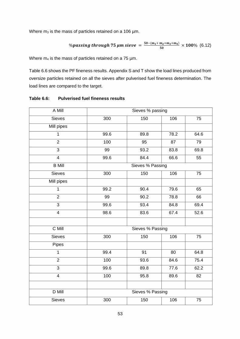
53
Where m3 is the mass of particles retained on a 106 µm.
%𝒑𝒂𝒔𝒔𝒊𝒏𝒈 𝒕𝒉𝒓𝒐𝒖𝒈𝒉 𝟕𝟓 𝝁𝒎 𝒔𝒊𝒆𝒗𝒆 = 𝟓𝟎−(𝒎𝟏+ 𝒎𝟐+𝒎𝟑+𝒎𝟒)
𝟓𝟎 × 𝟏𝟎𝟎% (6.12)
Where m4 is the mass of particles retained on a 75 µm.
Table 6.6 shows the PF fineness results. Appendix S and T show the load lines produced from
oversize particles retained on all the sieves after pulverised fuel fineness determination. The
load lines are compared to the target.
Table 6.6: Pulverised fuel fineness results
A Mill Sieves % passing
Sieves 300 150 106 75
Mill pipes
1 99.6 89.8 78.2 64.6
2 100 95 87 79
3 99 93.2 83.8 69.8
4 99.6 84.4 66.6 55
B Mill Sieves % Passing
Sieves 300 150 106 75
Mill pipes
1 99.2 90.4 79.6 65
2 99 90.2 78.8 66
3 99.6 93.4 84.8 69.4
4 98.6 83.6 67.4 52.6
C Mill Sieves % Passing
Sieves 300 150 106 75
Pipes
1 99.4 91 80 64.8
2 100 93.6 84.6 75.4
3 99.6 89.8 77.6 62.2
4 100 95.8 89.6 82
D Mill Sieves % Passing
Sieves 300 150 106 75
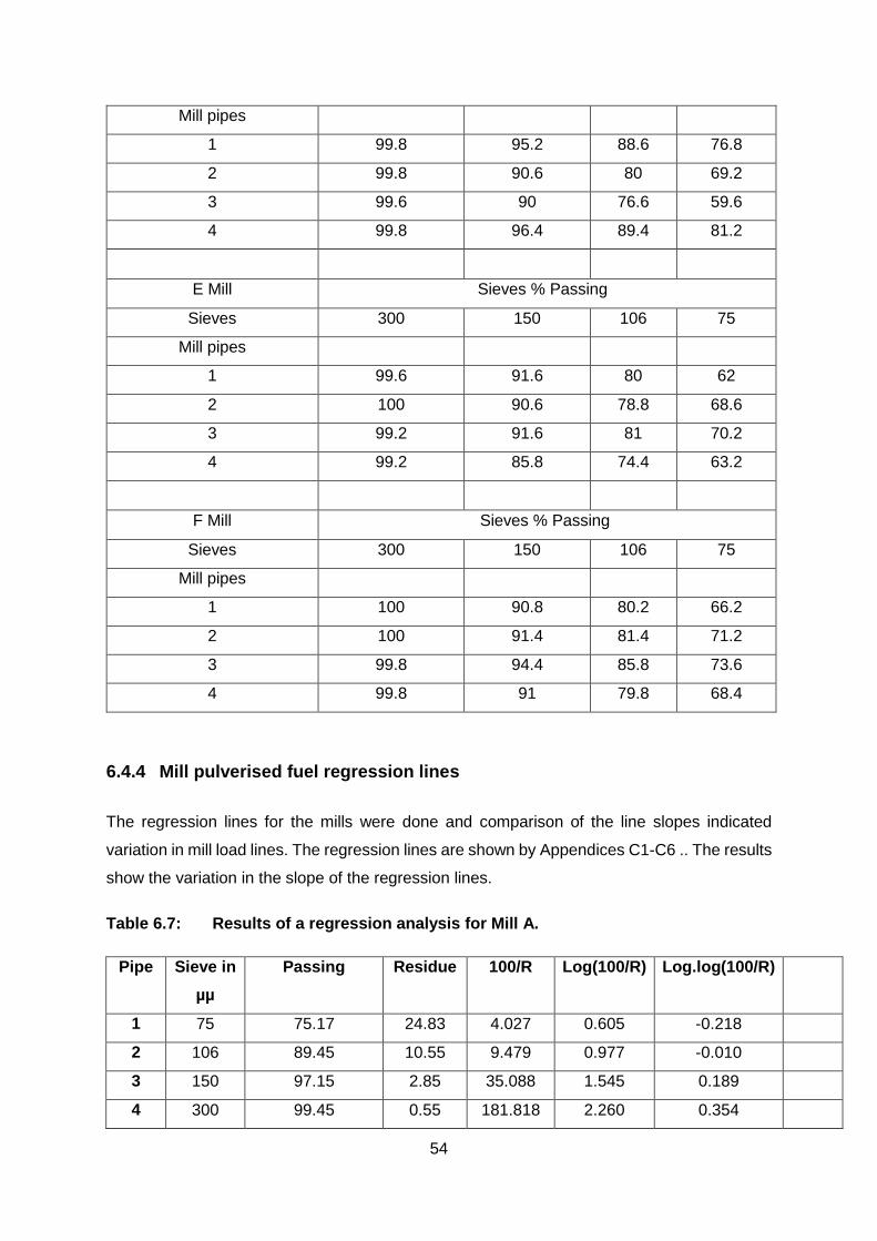
54
Mill pipes
1 99.8 95.2 88.6 76.8
2 99.8 90.6 80 69.2
3 99.6 90 76.6 59.6
4 99.8 96.4 89.4 81.2
E Mill Sieves % Passing
Sieves 300 150 106 75
Mill pipes
1 99.6 91.6 80 62
2 100 90.6 78.8 68.6
3 99.2 91.6 81 70.2
4 99.2 85.8 74.4 63.2
F Mill Sieves % Passing
Sieves 300 150 106 75
Mill pipes
1 100 90.8 80.2 66.2
2 100 91.4 81.4 71.2
3 99.8 94.4 85.8 73.6
4 99.8 91 79.8 68.4
6.4.4 Mill pulverised fuel regression lines
The regression lines for the mills were done and comparison of the line slopes indicated
variation in mill load lines. The regression lines are shown by Appendices C1-C6 .. The results
show the variation in the slope of the regression lines.
Table 6.7: Results of a regression analysis for Mill A.
Pipe Sieve in
µµ
Passing Residue 100/R Log(100/R) Log.log(100/R)
1 75 75.17 24.83 4.027 0.605 -0.218
2 106 89.45 10.55 9.479 0.977 -0.010
3 150 97.15 2.85 35.088 1.545 0.189
4 300 99.45 0.55 181.818 2.260 0.354
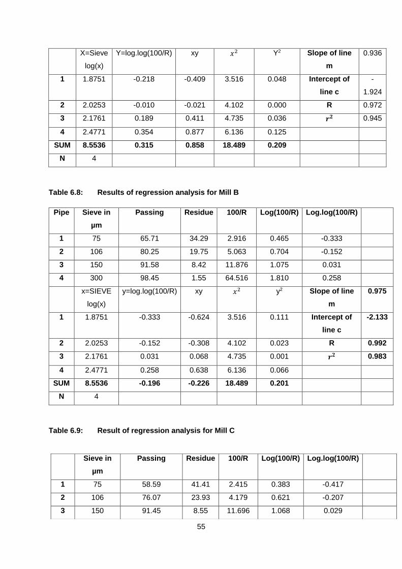
55
X=Sieve
log(x)
Y=log.log(100/R) xy 𝑥2 Y2 Slope of line
m
0.936
1 1.8751 -0.218 -0.409 3.516 0.048 Intercept of
line c
-
1.924
2 2.0253 -0.010 -0.021 4.102 0.000 R 0.972
3 2.1761 0.189 0.411 4.735 0.036 𝒓𝟐 0.945
4 2.4771 0.354 0.877 6.136 0.125
SUM 8.5536 0.315 0.858 18.489 0.209
N 4
Table 6.8: Results of regression analysis for Mill B
Pipe Sieve in
µm
Passing Residue 100/R Log(100/R) Log.log(100/R)
1 75 65.71 34.29 2.916 0.465 -0.333
2 106 80.25 19.75 5.063 0.704 -0.152
3 150 91.58 8.42 11.876 1.075 0.031
4 300 98.45 1.55 64.516 1.810 0.258
x=SIEVE
log(x)
y=log.log(100/R) xy 𝑥2 y2 Slope of line
m
0.975
1 1.8751 -0.333 -0.624 3.516 0.111 Intercept of
line c
-2.133
2 2.0253 -0.152 -0.308 4.102 0.023 R 0.992
3 2.1761 0.031 0.068 4.735 0.001 𝒓𝟐 0.983
4 2.4771 0.258 0.638 6.136 0.066
SUM 8.5536 -0.196 -0.226 18.489 0.201
N 4
Table 6.9: Result of regression analysis for Mill C
Sieve in
µm
Passing Residue 100/R Log(100/R) Log.log(100/R)
1 75 58.59 41.41 2.415 0.383 -0.417
2 106 76.07 23.93 4.179 0.621 -0.207
3 150 91.45 8.55 11.696 1.068 0.029
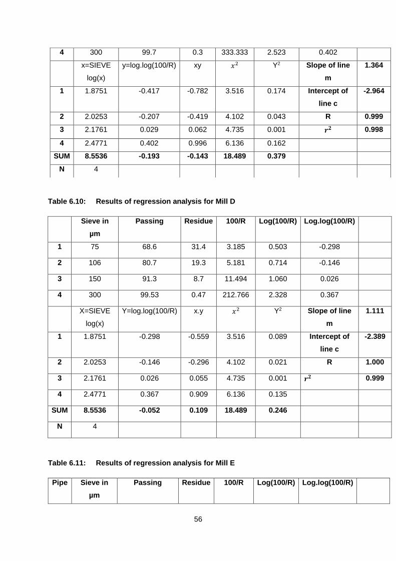
56
Table 6.10: Results of regression analysis for Mill D
Sieve in
µm
Passing Residue 100/R Log(100/R) Log.log(100/R)
1 75 68.6 31.4 3.185 0.503 -0.298
2 106 80.7 19.3 5.181 0.714 -0.146
3 150 91.3 8.7 11.494 1.060 0.026
4 300 99.53 0.47 212.766 2.328 0.367
X=SIEVE
log(x)
Y=log.log(100/R) x.y 𝑥2 Y2 Slope of line
m
1.111
1 1.8751 -0.298 -0.559 3.516 0.089 Intercept of
line c
-2.389
2 2.0253 -0.146 -0.296 4.102 0.021 R 1.000
3 2.1761 0.026 0.055 4.735 0.001 𝒓𝟐 0.999
4 2.4771 0.367 0.909 6.136 0.135
SUM 8.5536 -0.052 0.109 18.489 0.246
N 4
Table 6.11: Results of regression analysis for Mill E
Pipe Sieve in
µm
Passing Residue 100/R Log(100/R) Log.log(100/R)
4 300 99.7 0.3 333.333 2.523 0.402
x=SIEVE
log(x)
y=log.log(100/R) xy 𝑥2 Y2 Slope of line
m
1.364
1 1.8751 -0.417 -0.782 3.516 0.174 Intercept of
line c
-2.964
2 2.0253 -0.207 -0.419 4.102 0.043 R 0.999
3 2.1761 0.029 0.062 4.735 0.001 𝒓𝟐 0.998
4 2.4771 0.402 0.996 6.136 0.162
SUM 8.5536 -0.193 -0.143 18.489 0.379
N 4
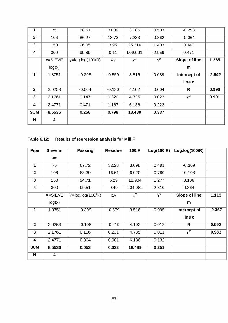
57
1 75 68.61 31.39 3.186 0.503 -0.298
2 106 86.27 13.73 7.283 0.862 -0.064
3 150 96.05 3.95 25.316 1.403 0.147
4 300 99.89 0.11 909.091 2.959 0.471
x=SIEVE
log(x)
y=log.log(100/R) Xy 𝑥2 y2 Slope of line
m
1.265
1 1.8751 -0.298 -0.559 3.516 0.089 Intercept of
line c
-2.642
2 2.0253 -0.064 -0.130 4.102 0.004 R 0.996
3 2.1761 0.147 0.320 4.735 0.022 𝒓𝟐 0.991
4 2.4771 0.471 1.167 6.136 0.222
SUM 8.5536 0.256 0.798 18.489 0.337
N 4
Table 6.12: Results of regression analysis for Mill F
Pipe Sieve in
µm
Passing Residue 100/R Log(100/R) Log.log(100/R)
1 75 67.72 32.28 3.098 0.491 -0.309
2 106 83.39 16.61 6.020 0.780 -0.108
3 150 94.71 5.29 18.904 1.277 0.106
4 300 99.51 0.49 204.082 2.310 0.364
X=SIEVE
log(x)
Y=log.log(100/R) x.y 𝑥2 Y2 Slope of line
m
1.113
1 1.8751 -0.309 -0.579 3.516 0.095 Intercept of
line c
-2.367
2 2.0253 -0.108 -0.219 4.102 0.012 R 0.992
3 2.1761 0.106 0.231 4.735 0.011 𝒓𝟐 0.983
4 2.4771 0.364 0.901 6.136 0.132
SUM 8.5536 0.053 0.333 18.489 0.251
N 4
58
6.4.5 Pulverised fuel Isokinetic sampling results discussion
The velocities of primary air and coal mixtures are measured in the pulverised fuel pipes. The
pulverised fuel flow velocities have maximums and minimums that are required during
operation of the mill. The Power Utility pulverised fuel velocities are:
conveying pipes feet per second minimum load 60-64. The conversion factor is 1ft =
0.3048m;
design is 89-96 feet per second;
minimum load pulverised fuel air mixture velocity is 18.288 - 19.507m/s and the design
maximum is 27.127 – 29.26 m/s; and
the burner nozzle flow velocities are 18.897 m/s minimum and design 35.052 m/s.
The mill pulverised fuel sampling tests were carried out and the following result was calculated
from the test data. The main aims of sampling pulverised fuel from pipes are:
coal flow through the mill;
air flow through the mill;
particle carrying velocities;
pulverised fuel mass flow and distribution;
mill performance evaluation; and
pulverised fuel fineness.
The mill pulverised fuel and air mixture velocities calculated from the data measured in the
pipes are:
pipe 1 = 27 m/s;
pipe 2 = 27m/s;
pipe 3 = 29 m/s; and
pipe 4 = 26 m/s.
59
The pulverised fuel fineness distribution to each pipe, the 75 µm sieve under sizing:
pipe 1 = 64.6%;
pipe 2 =79%;
pipe 3 = 69.8%; and
pipe 4 = 55%.
The coal flow in each pipe kg/s:
pipe1 = 1.0 kg/s
pipe2 = 1.1 kg/s
pipe 3 = 1.1 kg/s and
pipe 4 = 1.1 kg/s
The mill pipe velocity is at maximum flow at a load of 4.3 kg/s and the pulverised fuel fineness
is below design value 64.6%, passing in Pipe 1 and 55% in Pipe 4. The two pipes (2 and 3)
are 79 and 69.8% respectively. The fineness distribution is not the same in the four pipes. The
coal distribution in the pipes is 1.0 kg/s in Pipe 1 and 1.1 kg/s in Pipes 3 to Pipe 4.
The average fineness from the mill is 67.1%, this is lower than the design value of 70% through
the 75µm sieve.
The mill operating velocities are above the minimum pulverised fuel settling velocity:
Mill F = 37.5 m/s
Mill E = 32.25 m/s
Mill D = 27.25 m/s
Mill = 28 m/s
The mills on Unit 4 at Power Utility X are operating at velocities higher than the maximum of
27m/s - 29 m/s.
The regression for pulverised fuel fineness was done and the slope of the lines are shown by
Appendices C1-C6. The regression checks are shown by appendices B1-B4.
60
The regression lines gradients for the mills are as follows:
Mill A = 0.936;
Mill B = 0.992;
Mill C = 1.364;
Mill D = 1.111 and
Mill E = 1.265
6.5 Conclusion
The mill pulverised fuel sampling has been done and the distribution in pipes determined. The
fineness of the pulverised fuel in pipes has been found to differ. This is due to the mill operating
at high pulverised fuel air velocities. The high velocities’ result in changing the cut velocity of
the mill and coarser particles are entrained in the high velocity air. Mill A on Unit 4 operates in
relation with the other four mills.
The mills’ classifier angles settings are at 40-degrees instead of 35-degrees, as was used in
acceptance testing. Changing the gradients of the mill’s regression lines impacts on mill load
lines, mill output and pulverised coal fineness.
The pulverised fuel fineness has impact on the mill capacity. The graph above shows the
impact of coal fineness on mill capacity.

61
7 Mill power consumption and heat balance Excel spreadsheets
7.1 Introduction
The aim of this study is to perform an investigation of the effect of coal feedstock property
variation on the vertical spindle coal pulverising mill performance to facilitate optimal plant
performance. The purpose of this chapter is to develop two Excel spreadsheet programs that
calculate mill power consumption and mill heat balance, respectively.
7.2 Mill power consumption
Mill operation uses electric power which is part of the power generated from the unit. This
power, if not controlled, could exceed the design value. Values of power consumption above
design reduce the power sent out to the customer. The power consumed by milling plants
during power generation is part of the efficiency calculation input data. A high input of mill
power consumption reduces the efficiency of the generating unit.
The mill power consumption Excel program is developed using the following equations: 2.22,
equation 2.23, equation 2.24, and equation 2.25. The program input parameters are:
Primary air flow rate;
primary air temperature;
primary air pressure;
pulverised fuel fineness %; and
force on each grinding ball.
The program results are: mill frictional factor, mill power-draw, cut velocity and cut diameter.
The input parameters are varied from upper to lower values to evaluate the effect on mill
power-draw, mill frictional factor, cut velocity and cut diameters.
7.3 Mill power consumption Excel spreadsheet results
The data in table were calculated by the Excel spreadsheet. The calculated data is compared
to Power Utility data calculated by the spreadsheet. The spreadsheet is calibrated with mill
data and mill dimensions. Using this program, calibration to the mill data impacts the accuracy
of the output data. The parameters in are in Table 7.1.
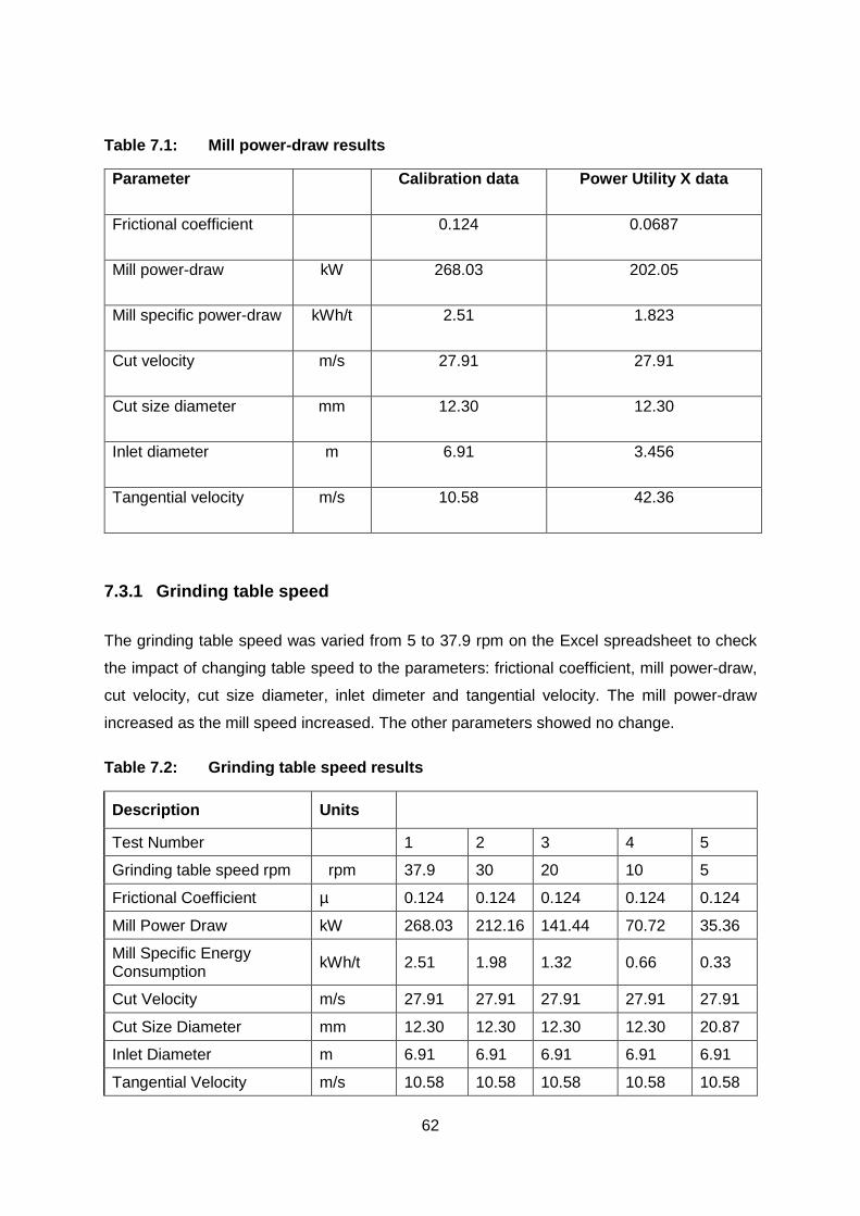
62
Table 7.1: Mill power-draw results
Parameter Calibration data Power Utility X data
Frictional coefficient 0.124 0.0687
Mill power-draw kW 268.03 202.05
Mill specific power-draw kWh/t 2.51 1.823
Cut velocity m/s 27.91 27.91
Cut size diameter mm 12.30 12.30
Inlet diameter m 6.91 3.456
Tangential velocity m/s 10.58 42.36
7.3.1 Grinding table speed
The grinding table speed was varied from 5 to 37.9 rpm on the Excel spreadsheet to check
the impact of changing table speed to the parameters: frictional coefficient, mill power-draw,
cut velocity, cut size diameter, inlet dimeter and tangential velocity. The mill power-draw
increased as the mill speed increased. The other parameters showed no change.
Table 7.2: Grinding table speed results
Description Units
Test Number 1 2 3 4 5
Grinding table speed rpm rpm 37.9 30 20 10 5
Frictional Coefficient µ 0.124 0.124 0.124 0.124 0.124
Mill Power Draw kW 268.03 212.16 141.44 70.72 35.36
Mill Specific Energy Consumption
kWh/t 2.51 1.98 1.32 0.66 0.33
Cut Velocity m/s 27.91 27.91 27.91 27.91 27.91
Cut Size Diameter mm 12.30 12.30 12.30 12.30 20.87
Inlet Diameter m 6.91 6.91 6.91 6.91 6.91
Tangential Velocity m/s 10.58 10.58 10.58 10.58 10.58
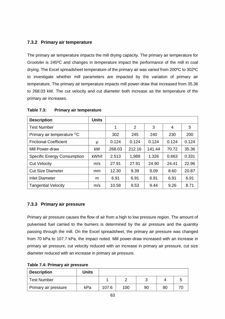
63
7.3.2 Primary air temperature
The primary air temperature impacts the mill drying capacity. The primary air temperature for
Grootvlei is 245ºC and changes in temperature impact the performance of the mill in coal
drying. The Excel spreadsheet temperature of the primary air was varied from 200ºC to 302ºC
to investigate whether mill parameters are impacted by the variation of primary air
temperature. The primary air temperature impacts mill power-draw that increased from 35.36
to 268.03 kW. The cut velocity and cut diameter both increase as the temperature of the
primary air increases.
Table 7.3: Primary air temperature
Description Units
Test Number
1 2 3 4 5
Primary air temperature OC
302 245 240 230 200
Frictional Coefficient µ 0.124 0.124 0.124 0.124 0.124
Mill Power-draw kW 268.03 212.16 141.44 70.72 35.36
Specific Energy Consumption kWh/t 2.513 1,989 1.326 0.663 0.331
Cut Velocity m/s 27.91 27.91 24.90 24.41 22.96
Cut Size Diameter mm 12.30 9.39 9.09 8.60 20.87
Inlet Diameter m 6.91 6.91 6.91 6.91 6.91
Tangential Velocity m/s 10.58 9.53 9.44 9.26 8.71
7.3.3 Primary air pressure
Primary air pressure causes the flow of air from a high to low pressure region. The amount of
pulverised fuel carried to the burners is determined by the air pressure and the quantity
passing through the mill. On the Excel spreadsheet, the primary air pressure was changed
from 70 kPa to 107.7 kPa, the impact noted. Mill power-draw increased with an increase in
primary air pressure, cut velocity reduced with an increase in primary air pressure, cut size
diameter reduced with an increase in primary air pressure.
Table 7.4: Primary air pressure
Description Units
Test Number
1 2 3 4 5
Primary air pressure kPa 107.6 100 90 80 70
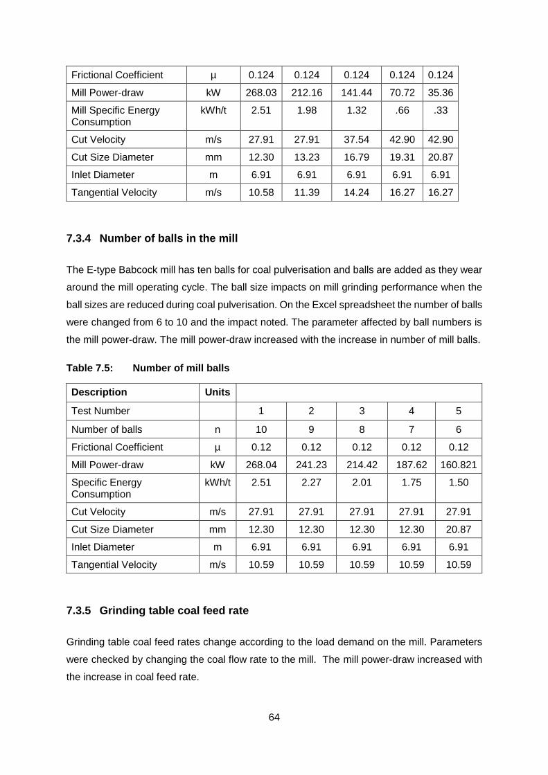
64
Frictional Coefficient µ 0.124 0.124 0.124 0.124 0.124
Mill Power-draw kW 268.03 212.16 141.44 70.72 35.36
Mill Specific Energy Consumption
kWh/t 2.51 1.98 1.32 .66 .33
Cut Velocity m/s 27.91 27.91 37.54 42.90 42.90
Cut Size Diameter mm 12.30 13.23 16.79 19.31 20.87
Inlet Diameter m 6.91 6.91 6.91 6.91 6.91
Tangential Velocity m/s 10.58 11.39 14.24 16.27 16.27
7.3.4 Number of balls in the mill
The E-type Babcock mill has ten balls for coal pulverisation and balls are added as they wear
around the mill operating cycle. The ball size impacts on mill grinding performance when the
ball sizes are reduced during coal pulverisation. On the Excel spreadsheet the number of balls
were changed from 6 to 10 and the impact noted. The parameter affected by ball numbers is
the mill power-draw. The mill power-draw increased with the increase in number of mill balls.
Table 7.5: Number of mill balls
Description Units
Test Number
1 2 3 4 5
Number of balls n 10 9 8 7 6
Frictional Coefficient µ 0.12 0.12 0.12 0.12 0.12
Mill Power-draw kW 268.04 241.23 214.42 187.62 160.821
Specific Energy Consumption
kWh/t 2.51 2.27 2.01 1.75 1.50
Cut Velocity m/s 27.91 27.91 27.91 27.91 27.91
Cut Size Diameter mm 12.30 12.30 12.30 12.30 20.87
Inlet Diameter m 6.91 6.91 6.91 6.91 6.91
Tangential Velocity m/s 10.59 10.59 10.59 10.59 10.59
7.3.5 Grinding table coal feed rate
Grinding table coal feed rates change according to the load demand on the mill. Parameters
were checked by changing the coal flow rate to the mill. The mill power-draw increased with
the increase in coal feed rate.
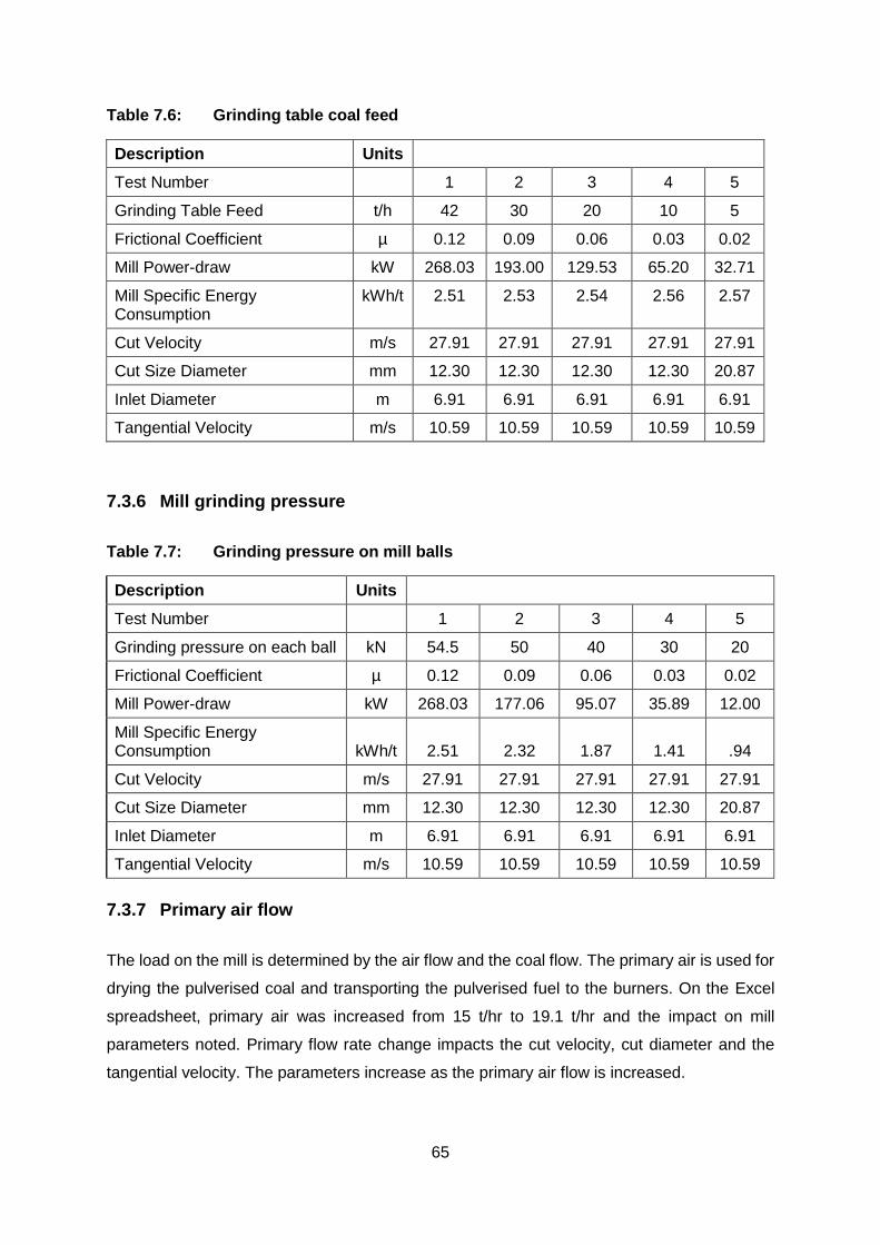
65
Table 7.6: Grinding table coal feed
Description Units
Test Number
1 2 3 4 5
Grinding Table Feed t/h 42 30 20 10 5
Frictional Coefficient µ 0.12 0.09 0.06 0.03 0.02
Mill Power-draw kW 268.03 193.00 129.53 65.20 32.71
Mill Specific Energy Consumption
kWh/t 2.51 2.53 2.54 2.56 2.57
Cut Velocity m/s 27.91 27.91 27.91 27.91 27.91
Cut Size Diameter mm 12.30 12.30 12.30 12.30 20.87
Inlet Diameter m 6.91 6.91 6.91 6.91 6.91
Tangential Velocity m/s 10.59 10.59 10.59 10.59 10.59
7.3.6 Mill grinding pressure
Table 7.7: Grinding pressure on mill balls
Description Units
Test Number
1 2 3 4 5
Grinding pressure on each ball kN 54.5 50 40 30 20
Frictional Coefficient µ 0.12 0.09 0.06 0.03 0.02
Mill Power-draw kW 268.03 177.06 95.07 35.89 12.00
Mill Specific Energy Consumption kWh/t 2.51 2.32 1.87 1.41 .94
Cut Velocity m/s 27.91 27.91 27.91 27.91 27.91
Cut Size Diameter mm 12.30 12.30 12.30 12.30 20.87
Inlet Diameter m 6.91 6.91 6.91 6.91 6.91
Tangential Velocity m/s 10.59 10.59 10.59 10.59 10.59
7.3.7 Primary air flow
The load on the mill is determined by the air flow and the coal flow. The primary air is used for
drying the pulverised coal and transporting the pulverised fuel to the burners. On the Excel
spreadsheet, primary air was increased from 15 t/hr to 19.1 t/hr and the impact on mill
parameters noted. Primary flow rate change impacts the cut velocity, cut diameter and the
tangential velocity. The parameters increase as the primary air flow is increased.
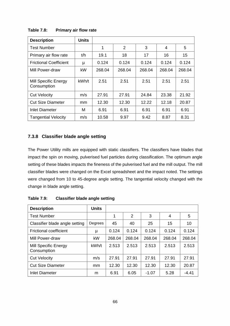
66
Table 7.8: Primary air flow rate
Description Units
Test Number
1 2 3 4 5
Primary air flow rate t/h 19.1 18 17 16 15
Frictional Coefficient µ 0.124 0.124 0.124 0.124 0.124
Mill Power-draw kW 268.04 268.04 268.04 268.04 268.04
Mill Specific Energy Consumption
kWh/t 2.51 2.51 2.51 2.51 2.51
Cut Velocity m/s 27.91 27.91 24.84 23.38 21.92
Cut Size Diameter mm 12.30 12.30 12.22 12.18 20.87
Inlet Diameter M 6.91 6.91 6.91 6.91 6.91
Tangential Velocity m/s 10.58 9.97 9.42 8.87 8.31
7.3.8 Classifier blade angle setting
The Power Utility mills are equipped with static classifiers. The classifiers have blades that
impact the spin on moving, pulverised fuel particles during classification. The optimum angle
setting of these blades impacts the fineness of the pulverised fuel and the mill output. The mill
classifier blades were changed on the Excel spreadsheet and the impact noted. The settings
were changed from 10 to 45-degree angle setting. The tangential velocity changed with the
change in blade angle setting.
Table 7.9: Classifier blade angle setting
Description Units
Test Number
1 2 3 4 5
Classifier blade angle setting Degrees 45 40 25 15 10
Frictional coefficient µ 0.124 0.124 0.124 0.124 0.124
Mill Power-draw kW 268.04 268.04 268.04 268.04 268.04
Mill Specific Energy Consumption
kWh/t 2.513 2.513 2.513 2.513 2.513
Cut Velocity m/s 27.91 27.91 27.91 27.91 27.91
Cut Size Diameter mm 12.30 12.30 12.30 12.30 20.87
Inlet Diameter m 6.91 6.05 -1.07 5.28 -4.41
67
7.4 Mill power consumption Excel spreadsheet result’s discussion
The cut velocity and cut diameter increase as the air increases due to temperature. When cut
velocity increases, pulverised fuel classification coarse particles entrainment to the burners
occurs. The reduction in pulverised fuel fineness results in flame instability.
The grinding table coal feed rate impact is that the mill power-draw increases recirculation
load. The recirculation load is coal feed, mill classifier rejects and elutriator rejects. The
recirculation load increases with the coal flow rate increase.
Mill grinding pressure impacts mill power-draw increases, with the increase in frictional forces.
The primary air flow impacts on mill power-draw and the cut velocity and cut diameter. The
high primary air flows entrain coarse particles of pulverised fuel to the burners. The mill output
reduces with coarse particle entrainment, increasing the feed flow results and causing a mill
power-draw increase.
Classifier blades angle settings impact pulverised fuel classification and fineness of said
pulverised fuel. Optimum position is determined by pulverised fuel sampling and grading. The
optimum fineness determines the position of the classifier setting.
7.5 Mill heat balance
The purpose of this section is to develop a heat balance Excel spreadsheet program, that
calculates mill heat balance.
The heat balance of the mill can be used to evaluate mill parameters during operation. The
heat balance evaluation enables the assessment of the mill drying constraint that exists during
operation. The parameters that impact on the drying capacity of the mill are moisture content
of coal and the primary air temperature. The Power Utility X design’s coal moisture content is
10% total moisture. Should moisture content of coal value more than 10%, (coal drying is not
a constraint) the mill output is reduced due to the extended time of drying the coal. The mill
heat balance evaluates the energy going into the mill and the energy out of the mill.
7.6 Mill heat balance Excel spreadsheet results.
The heat balance Excel spreadsheet was modelled using Equations 2.10 to 2.21. Table 7.9
shows the mill heat balance Excel spreadsheet results. Figure 7.1 shows the mill heat balance.
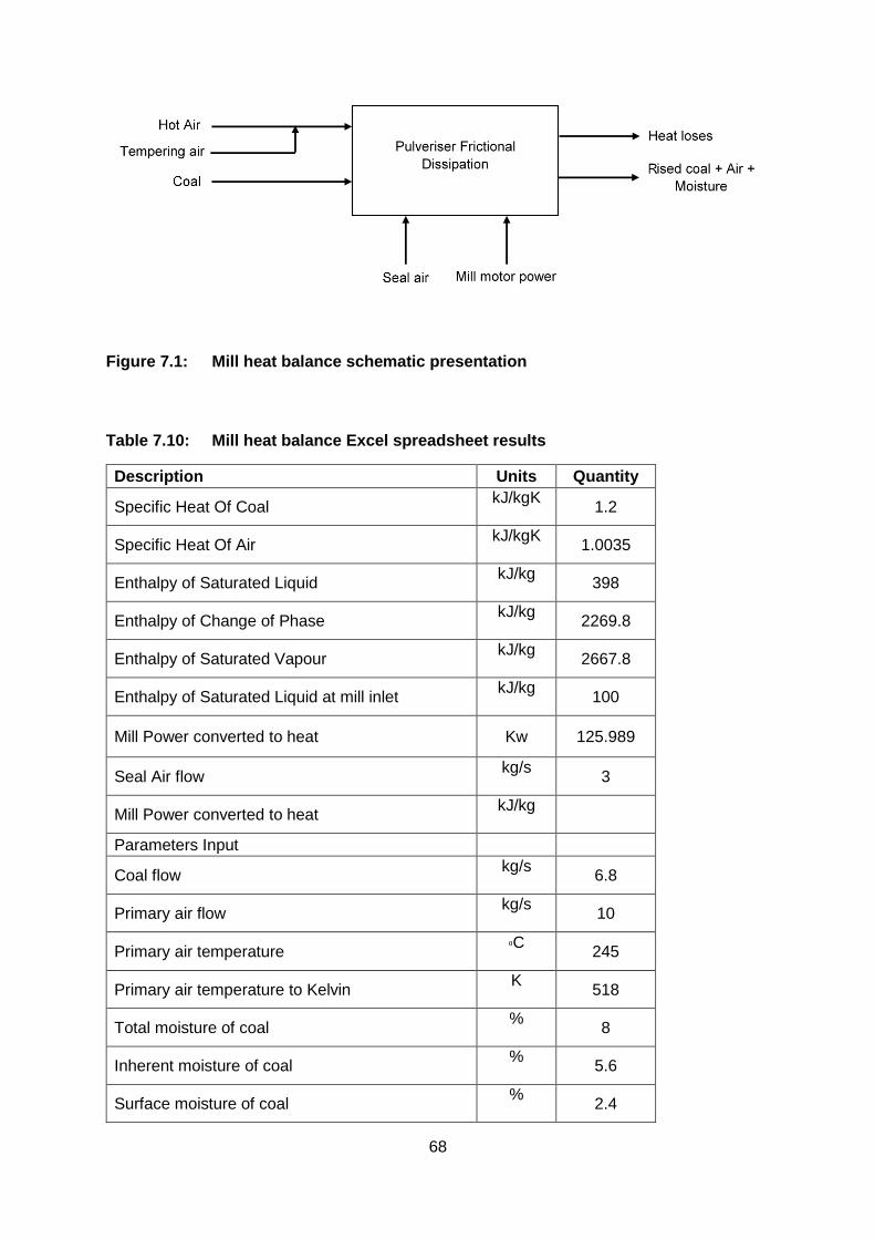
68
Figure 7.1: Mill heat balance schematic presentation
Table 7.10: Mill heat balance Excel spreadsheet results
Description Units Quantity
Specific Heat Of Coal kJ/kgK
1.2
Specific Heat Of Air kJ/kgK
1.0035
Enthalpy of Saturated Liquid kJ/kg
398
Enthalpy of Change of Phase kJ/kg
2269.8
Enthalpy of Saturated Vapour kJ/kg
2667.8
Enthalpy of Saturated Liquid at mill inlet kJ/kg
100
Mill Power converted to heat Kw 125.989
Seal Air flow kg/s
3
Mill Power converted to heat kJ/kg
Parameters Input
Coal flow kg/s
6.8
Primary air flow kg/s
10
Primary air temperature ₀C
245
Primary air temperature to Kelvin K
518
Total moisture of coal %
8
Inherent moisture of coal %
5.6
Surface moisture of coal %
2.4
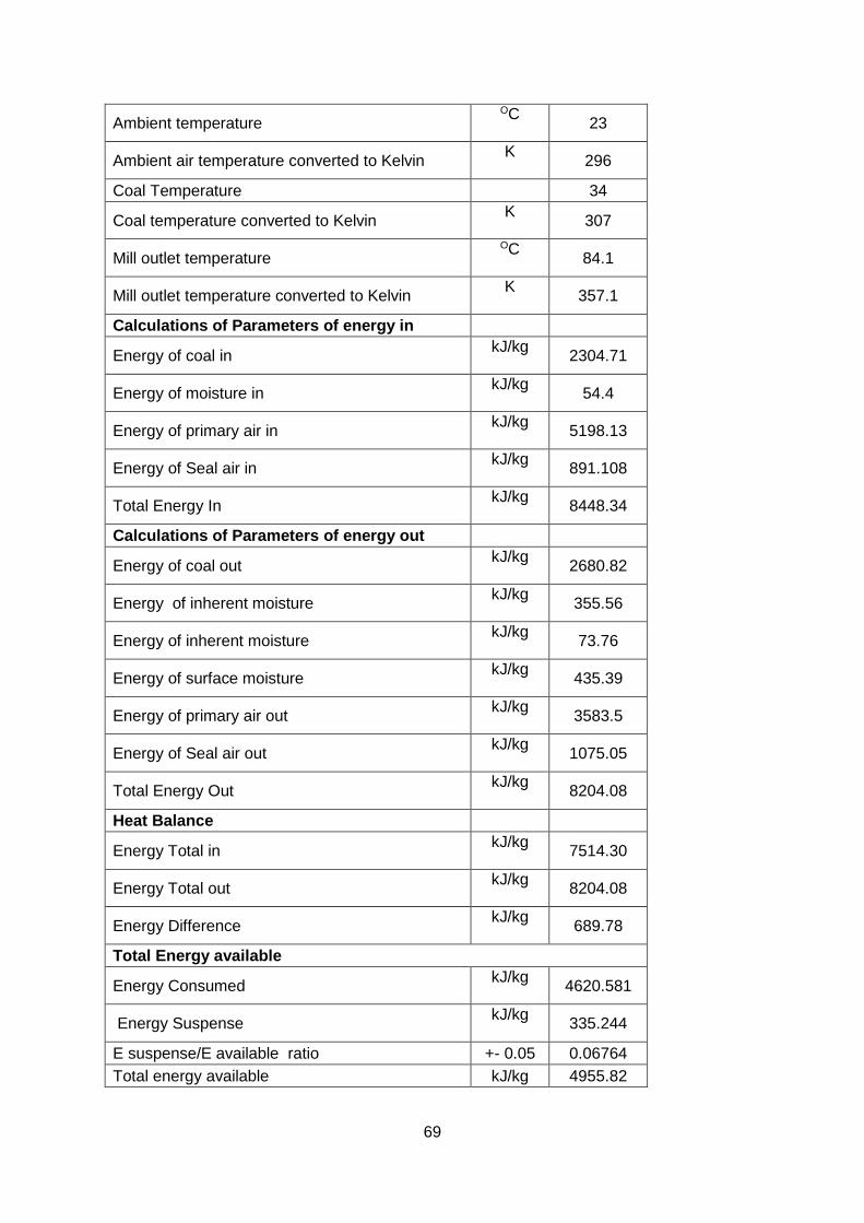
69
Ambient temperature OC
23
Ambient air temperature converted to Kelvin K
296
Coal Temperature 34
Coal temperature converted to Kelvin K
307
Mill outlet temperature OC
84.1
Mill outlet temperature converted to Kelvin K
357.1
Calculations of Parameters of energy in
Energy of coal in kJ/kg
2304.71
Energy of moisture in kJ/kg
54.4
Energy of primary air in kJ/kg
5198.13
Energy of Seal air in kJ/kg
891.108
Total Energy In kJ/kg
8448.34
Calculations of Parameters of energy out
Energy of coal out kJ/kg
2680.82
Energy of inherent moisture kJ/kg
355.56
Energy of inherent moisture kJ/kg
73.76
Energy of surface moisture kJ/kg
435.39
Energy of primary air out kJ/kg
3583.5
Energy of Seal air out kJ/kg
1075.05
Total Energy Out kJ/kg
8204.08
Heat Balance
Energy Total in kJ/kg
7514.30
Energy Total out kJ/kg
8204.08
Energy Difference kJ/kg
689.78
Total Energy available
Energy Consumed kJ/kg
4620.581
Energy Suspense kJ/kg
335.244
E suspense/E available ratio +- 0.05 0.06764
Total energy available kJ/kg 4955.82
70
7.6.1 Discussion of results
The heat balance Excel spreadsheet calculates the heat input to the mill for drying the
pulverised coal and the heat output of the mill. The total energy input to the mill was calculated
to be 7514.30 kJ/kg.
The total energy available was calculated and the value is 4955.82kJ/kg
The energy consumed by the mill is calculated by finding the difference between mill total
energy out and energy of primary air out. The consumed energy was evaluated to be
4620.58kJ/kg.
Energy suspense is calculated by taking the difference between total energy available and
energy consumed. The energy suspense calculated value is 335.24 kJ/kg.
The energy available is calculated by adding the energy of primary air in and mill power,
converted to heat. The mill’s available energy is 4955.82 kJ/kg.
The design ratio of energy suspense/energy available is +/- 0.05. The Excel spreadsheet
model gave an actual ratio of 0.067.
7.6.2 Conclusion
The mill’s pulverised fuel drying capacity is within design. The ratio of suspense energy and
energy available is 0.067, compared to the standard of 0.05. The moisture content of the coal
supply to the station is below 10%. The temperature of the primary air is 245ºC, which is also
the heat available to dry the coal. The mill’s pulverised fuel leaks need repair to prevent loss
of the heat in the primary air.
7.7 Load simulations
Load simulations were carried out on the mills to compare three sets of data:
Simulated coal flow/air flow;
sampled coal flow and air flow; and
control panel indicated coal and air flow.
. Appendix D shows the results of the load simulations.
71
The operator uses the coal flows indicated on the panel, the load simulations checked the
correctness of the instruments and the actual load in the plant. The measured data compared
with simulated and control room indications, which can be used as a check on control
instrumentation.
Mill load line evaluation is done by measuring the coal flow and the air flow.
7.7.1 Discussion of results
The comparison of simulated, sampled and control room loads provided a check on these
parameters. Unit operators rely on control room indications and when these are out of
calibration, decisions made based on these indications impact plant performance. Process
engineers, with the use of simulation Excel spreadsheets, can determine the loads on the
mills.
7.7.2 Conclusion
Load simulations were done and compared with sampled loads and control room indications.
The comparison provided data for accuracy of the isokinetic coal sampler and control room
indications.
72
8 Conclusions and recommendations
The present investigation of this dissertation was aimed at performance optimisation of vertical
spindle coal pulverisers. A detailed literature review was done to get an understanding of
principles of operations of the vertical spindle coal pulverisers. The literature review provided
data and information on vertical spindle coal pulverisers on processes and associated
components operations. The challenges associated with coal properties variation on
pulverisers operations were analysed in detail.
In order to optimise the performance of vertical spindle coal pulverizers, the operating
parameters should be monitored. The operational aspect of the mill must be understood in
order to relate the fundamental principles of operation to the vertical spindle coal pulverizers.
The performance optimisation of the vertical spindle coal pulverizers was investigated and to
achieve optimisation, the following was carried out:
Plant tests were conducted at Power Utility X Unit 4 mills A-F to evaluate plant performance
as related to fineness distribution, mill bias, mill throughput, mill outlet temperature, power
consumption, and reliability and pulverized fuel settling velocity.
Laboratory tests were conducted to determine coal fineness, calorific value of coal, Hardgrove
Grindability Index, Abrasion Index, ash and moisture content.
Abrasive Index was determined at the station and compared with the design coal. The coal
supply to the station comes from several mines. Contractually, the coal is blended to have ash
and calorific values within the contract upper- and lower limits. The values obtained during the
test show that the coal is abrasive. Abrasion Index shows that the coal can remove materials
on pipes, coal chutes and the mill during the coal grinding process impacting on mill
maintenance. The impact of a high Abrasive Index is the high cost of maintenance of the
associated plant milling, plant ducting and pipes handling the coal.
Hardgrove Grindability Index was determined at the station using station equipment. The
finding was that the Hardgrove Grindability Index of the coal supply to the station is not
constant. The test consisted of thirty samples representing thirty days of coal supply. The HGI
was varying as indicated by Figure 6.2. The coal with a high HGI is easy to grind and that with
a low HGI is difficult to grind. The HGI of coal has an impact on the mill output. The HGI is not
additive (ACARP, 1988:1-8) when coal is blended with coal of a different HGI.
The calorific value of coal was determined at the station and the trend showed the variation of
Calorific values of coal during the period of supply. The mills are designed to deliver the
73
required coal throughput for boiler energy required. Change in calorific value of coal means
change in energy content of the coal. When a low calorific value is experienced, the impact
on the mill is twofold. Low calorific value of coal means energy content is low; more coal is
required to match the load requirement. The second impact is that the mills grind more coal to
match the energy requirements. Mills are designed to provide 7kg/s of coal at full load at the
designed calorific value of coal.
Moisture content was determined at the station and the finding was that the moisture content
of coal during the dry season is less than 10%. The mill carries four functions at once: grinding
of coal, drying, classification and transportation of the pulverized coal to the burners. The
drying of the coal is impacted by the moisture content of coal and the inlet temperature of
primary air to the mill. The mill design and operating primary air temperature was evaluated
and is still operating as designed at the 245oC inlet temperature. The mill outlet temperatures
were observed to be 84ºC. The mill drying capacity is operating as designd when coal moisture
content is less than 10%. During the rainy season the wet coal management system ensures
that moisture content of coal on the stockpile is controlled by the drainage system.
The fineness distribution of pulverized coal, pulverized fuel burner distribution, mill bias, mill
throughput, mill outlet temperatures, power consumption and pulverized fuel settling velocities
tests were carried out. The findings were that fineness is not evenly distributed in the pipes
leading to the burners. The unit mass in pipes is not evenly distributed, some pipes are
carrying less fuel. The pipes with less fuel than air are operating lean. The pipes that are
carrying more fuel than air ratios recommended are said to be operating rich. The preferred
ratios are those that are termed ‘stoichiometric ratios’.
The velocities m/s in pipes of pulverized fuel were determined and analysed. The station
design fuel air velocities are 18.86 m/s minimum velocity. The mills operating below minimum
velocity will have fuel settling around bends, as velocity reduction occurs due to low pressure.
On the other hand, the maximum operating velocity design is 29.19 m/s. Velocities above the
maximum design values impact the mills, having coarser fuel particles carry-over to the
burners.
The wear rate of mills, pipes and ducting is proportional to the velocity of air carrying particles
(Gill, 1984: 347-353)
Coal feed rate to the mill is achieved by using a coal feeder. The station in question still uses
a table coal feeder. The table coal feeder has a table that has waffles to assist in feeding coal
to the mill. The feeding mechanism has a plough mechanism that is provided to plough an
74
amount of coal to the mill, depending on the amount of coal required. The plough action
coupled with the feeder speed regulation is meant to deliver the required coal. This system
has been fixed in position and the feeder uses the speed to deliver the coal required by the
mill to match the energy on the boiler. The mechanism opens and closes the gap of angle of
coal repose on the table. When more coal is required, the plough increases the angle of cutting
coal and the reverse is true when coal reduction is required. The plough mechanism operates
in tandem with the speed of the coal feeder. The increase in coal feeder speed is supposed
to increase the coal feed to the mill. The investigation finding was that the feeder plough is
now fixed and the coal quantity feed to the mill is only increased or decreased by the coal
feeder speed.
Mill control during operation is achieved by monitoring the following parameters:
Coal flow.
Air flow, primary air differential pressure.
Mill inlet temperature.
Mill outlet temperature.
Mill recirculation load - mill differential pressure.
Tempering air.
The mill outlet temperatures are controlled by regulating the coal flow and amount of tempering
air that is introduced to the primary air at the inlet, reducing temperature to desired value.
The investigation found that the mills are operating at a temperature of 84oC as the outlet
temperature and 245oC as the inlet temperature. The mill drying capacity is controlled within
the design limits.
The control of primary air differential pressure and mill differential pressure, provide data for
mill load line. This load line is used for checking the operating of the mill.
Two Excel spreadsheets were developed using equations in Chapter 2 and these
spreadsheets were used to evaluate mill heat losses and the effect of varying operating
parameters on a mill. Using these spreadsheets, assumptions are made on the steady state
operations of the mill. The mills are operating at equilibrium conditions and the mill dimensional
parameters are not changing during operations.
A mill power consumption spreadsheet was used to assess the effect of varying operating
parameters on the mill. The parameters that varied were:
Primary air temperature;
coal feed rate;

75
pressure on the mill balls;
primary air pressure;
mill rotation speed;
fineness of pulverised coal; and
mill classifier settings.
The impact on mill power draw was noted and changing operating parameters can be done
when optimisation has occurred.
The spreadsheet on mill heat balance and mill power consumption are usable for monitoring
coal pulveriser performance
8.1 Recommendations
Mill performance monitoring and optimisation programs improve mill output and operating load
lines, optimal operation reduces operating and maintenance costs.
76
References
Afolabi, L., Aroussi, A. & Isa, N.M. 2011. Numerical modelling of the carrier gas phase in a
laboratory-scale coal classifier model. Fuel Processing Technology, 92(3):556-562.
Arauzo, I. & Cortés, C. 1995. Diagnosis of milling systems performance based on operating
window and mill consumption correlations. (In Intersociety energy conversion engineering
conference organised by the American nuclear society. p. 397-397).
Association, B.C.U.R. & Field, M.A. 1967. Combustion of pulverised coal. British Coal
Utilisation Research Association.
Babcock Grootvlei Boiler 3 Operations Manual , Volume 4 Operating Procedures
Bhambare, K.S., Ma, Z. & Lu, P. 2010. CFD modeling of MPS coal mill with moisture
evaporation. Fuel Processing Technology, 91(5):566-571.
Fan, G. & Rees, N. 1994. Modelling of vertical spindle mill’s in coal fired power plants. (In
EEC 94: Electrical Engineering Congress 1994; Preprints; Enabling Technologies, Developing
Industry; Congress and Exhibition organised by: Institution of Engineers, Australia. p. 235).
Gill, A.B. 1984. Power plant performance. Amsterdam: Elsevier.
Holtshauzen, G. 2008. Coal pulveriser maintenance performance enhancement through the
application of a combination of new technologies. University of Johannesburg (Dissertation M
Eng).
Hukki, R. 1961. Proposal for a solomonic settlement between the theories of von Rittinger,
Kick and Bond. Trans. AIME, 220:403-408.
Jankovic, A., Dundar, H. & Mehta, R. 2010. Relationships between comminution energy and
product size for a magnetite ore. Journal of the South African Institute of Mining & Metallurgy,
110(3):141.
Kojovic, T., Shi, F. & Brennan, M. 2015. Modelling of vertical spindle mill’s. Part 2: Integrated
models for E-mill, MPS and CKP mill’s. Fuel, 143:602-611.
Lameck, N.N.S. 2006. Effects of grinding media shapes on ball mill performance. University
of the Witwatersrand, Johannesburg.
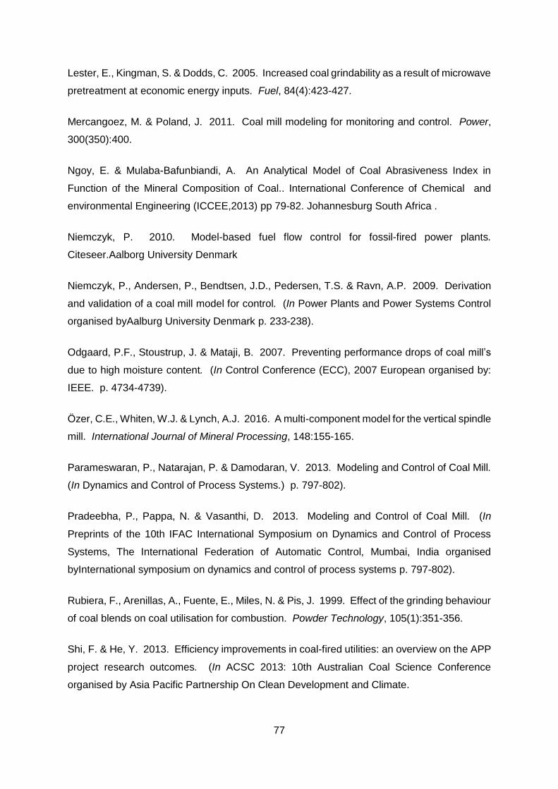
77
Lester, E., Kingman, S. & Dodds, C. 2005. Increased coal grindability as a result of microwave
pretreatment at economic energy inputs. Fuel, 84(4):423-427.
Mercangoez, M. & Poland, J. 2011. Coal mill modeling for monitoring and control. Power,
300(350):400.
Ngoy, E. & Mulaba-Bafunbiandi, A. An Analytical Model of Coal Abrasiveness Index in
Function of the Mineral Composition of Coal.. International Conference of Chemical and
environmental Engineering (ICCEE,2013) pp 79-82. Johannesburg South Africa .
Niemczyk, P. 2010. Model-based fuel flow control for fossil-fired power plants.
Citeseer.Aalborg University Denmark
Niemczyk, P., Andersen, P., Bendtsen, J.D., Pedersen, T.S. & Ravn, A.P. 2009. Derivation
and validation of a coal mill model for control. (In Power Plants and Power Systems Control
organised byAalburg University Denmark p. 233-238).
Odgaard, P.F., Stoustrup, J. & Mataji, B. 2007. Preventing performance drops of coal mill’s
due to high moisture content. (In Control Conference (ECC), 2007 European organised by:
IEEE. p. 4734-4739).
Özer, C.E., Whiten, W.J. & Lynch, A.J. 2016. A multi-component model for the vertical spindle
mill. International Journal of Mineral Processing, 148:155-165.
Parameswaran, P., Natarajan, P. & Damodaran, V. 2013. Modeling and Control of Coal Mill.
(In Dynamics and Control of Process Systems.) p. 797-802).
Pradeebha, P., Pappa, N. & Vasanthi, D. 2013. Modeling and Control of Coal Mill. (In
Preprints of the 10th IFAC International Symposium on Dynamics and Control of Process
Systems, The International Federation of Automatic Control, Mumbai, India organised
byInternational symposium on dynamics and control of process systems p. 797-802).
Rubiera, F., Arenillas, A., Fuente, E., Miles, N. & Pis, J. 1999. Effect of the grinding behaviour
of coal blends on coal utilisation for combustion. Powder Technology, 105(1):351-356.
Shi, F. & He, Y. 2013. Efficiency improvements in coal-fired utilities: an overview on the APP
project research outcomes. (In ACSC 2013: 10th Australian Coal Science Conference
organised by Asia Pacific Partnership On Clean Development and Climate.
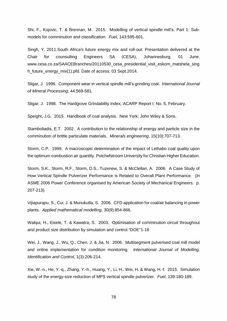
78
Shi, F., Kojovic, T. & Brennan, M. 2015. Modelling of vertical spindle mill’s. Part 1: Sub-
models for comminution and classification. Fuel, 143:595-601.
Singh, Y. 2011.South Africa's future energy mix and roll-out. Presentation delivered at the
Chair for counsulting Engineers SA (CESA), Johannesburg, 01 June.
www.cesa.co.za/SAACEBranches/20110530_cesa_presidential_visit_eskom_matshela_sing
h_future_energy_mix(1).pfd. Date of access: 03 Sept.2014.
Sligar, J. 1996. Component wear in vertical spindle mill’s grinding coal. International Journal
of Mineral Processing, 44:569-581.
Sligar, J. 1998. The Hardgrove Grindability Index, ACARP Report I. No. 5, February.
Speight, J.G. 2015. Handbook of coal analysis. New York: John Wiley & Sons.
Stamboliadis, E.T. 2002. A contribution to the relationship of energy and particle size in the
comminution of brittle particulate materials. Minerals engineering, 15(10):707-713.
Storm, C.P. 1999. A macroscopic determination of the impact of Lethabo coal quality upon
the optimum combustion air quantity. Potchefstroom University for Christian Higher Education.
Storm, S.K., Storm, R.F., Storm, D.S., Tuzenew, S. & McClellan, A. 2006. A Case Study of
How Vertical Spindle Pulverizer Performance is Related to Overall Plant Performance. (In
ASME 2006 Power Conference organised by American Society of Mechanical Engineers. p.
207-213).
Vijiapurapu, S., Cui, J. & Munukutla, S. 2006. CFD application for coal/air balancing in power
plants. Applied mathematical modelling, 30(9):854-866.
Walqui, H., Eisele, T. & Kawatra, S. 2003. Optimisation of comminution circuit throughout
and product size distribution by simulation and control."DOE"1-18
Wei, J., Wang, J., Wu, Q., Chen, J. & Jia, N. 2006. Multisegment pulverised coal mill model
and online implementation for condition monitoring. International Journal of Modelling,
Identification and Control, 1(3):206-214.
Xie, W.-n., He, Y.-q., Zhang, Y.-h., Huang, Y., Li, H., Wei, H. & Wang, H.-f. 2015. Simulation
study of the energy-size reduction of MPS vertical spindle pulverizer. Fuel, 139:180-189.
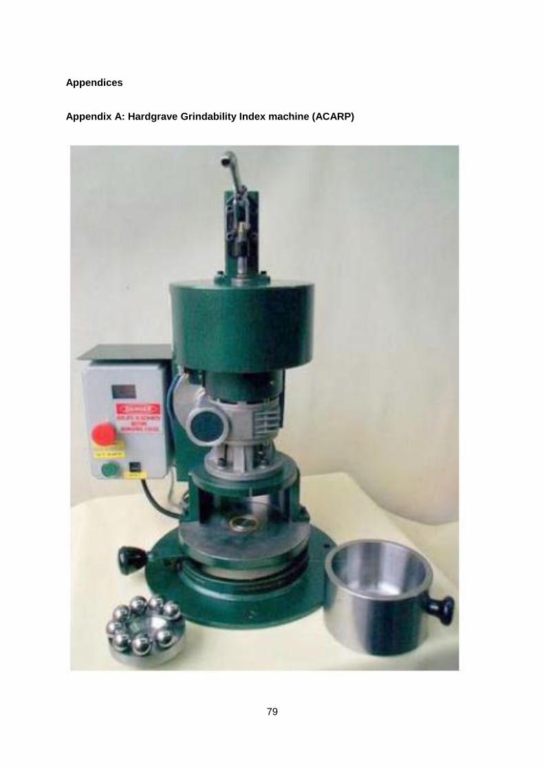
79
Appendices
Appendix A: Hardgrave Grindability Index machine (ACARP)
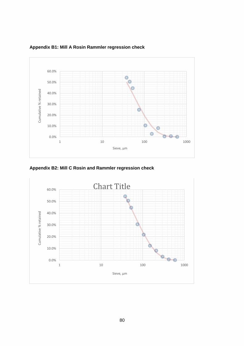
80
Appendix B1: Mill A Rosin Rammler regression check
Appendix B2: Mill C Rosin and Rammler regression check
0.0%
10.0%
20.0%
30.0%
40.0%
50.0%
60.0%
1 10 100 1000
Cu
mu
lati
ve %
ret
ain
ed
Sieve, µm
0.0%
10.0%
20.0%
30.0%
40.0%
50.0%
60.0%
1 10 100 1000
Cu
mu
lati
ve %
ret
ain
ed
Sieve, µm
Chart Title
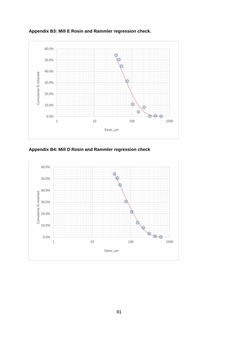
81
Appendix B3: Mill E Rosin and Rammler regression check.
Appendix B4: Mill D Rosin and Rammler regression check
0.0%
10.0%
20.0%
30.0%
40.0%
50.0%
60.0%
1 10 100 1000
Cu
mu
lati
ve %
ret
ain
ed
Sieve, µm
0.0%
10.0%
20.0%
30.0%
40.0%
50.0%
60.0%
1 10 100 1000
Cu
mu
lati
ve %
ret
ain
ed
Sieve, µm
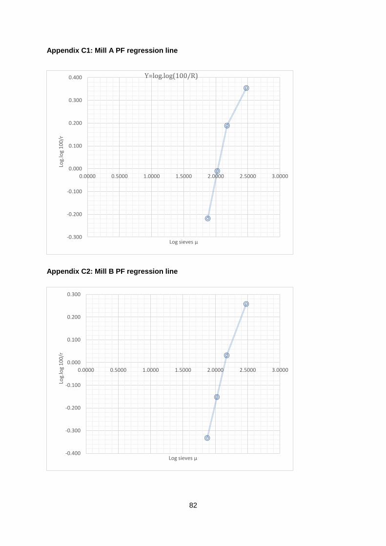
82
Appendix C1: Mill A PF regression line
Appendix C2: Mill B PF regression line
-0.300
-0.200
-0.100
0.000
0.100
0.200
0.300
0.400
0.0000 0.5000 1.0000 1.5000 2.0000 2.5000 3.0000
Log.
log
10
0/r
Log sieves µ
Y=log.log(100/R)
-0.400
-0.300
-0.200
-0.100
0.000
0.100
0.200
0.300
0.0000 0.5000 1.0000 1.5000 2.0000 2.5000 3.0000
Log.
log
10
0/r
Log sieves µ
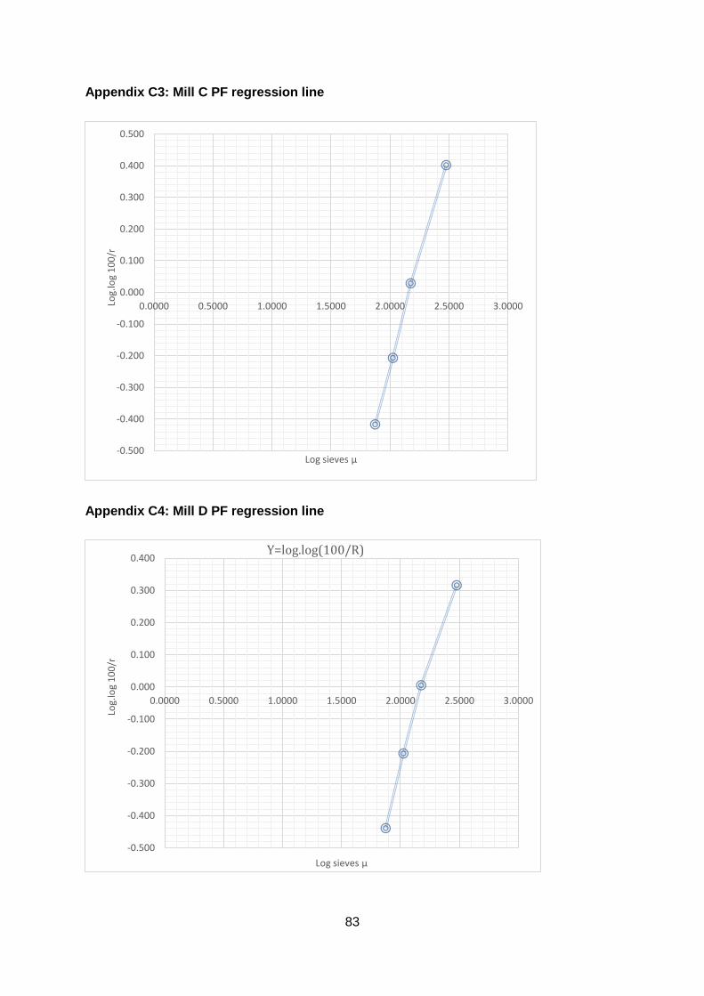
83
Appendix C3: Mill C PF regression line
Appendix C4: Mill D PF regression line
-0.500
-0.400
-0.300
-0.200
-0.100
0.000
0.100
0.200
0.300
0.400
0.500
0.0000 0.5000 1.0000 1.5000 2.0000 2.5000 3.0000Log.
log
10
0/r
Log sieves µ
-0.500
-0.400
-0.300
-0.200
-0.100
0.000
0.100
0.200
0.300
0.400
0.0000 0.5000 1.0000 1.5000 2.0000 2.5000 3.0000
Log.
log
10
0/r
Log sieves µ
Y=log.log(100/R)
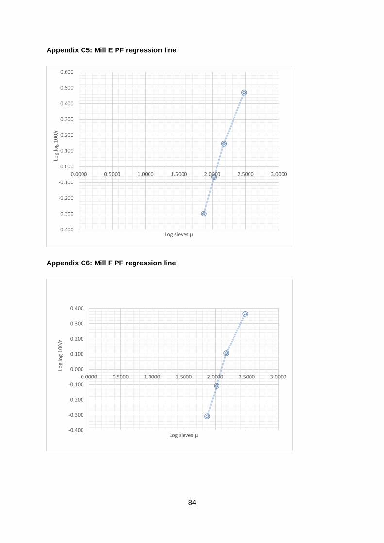
84
Appendix C5: Mill E PF regression line
Appendix C6: Mill F PF regression line
-0.400
-0.300
-0.200
-0.100
0.000
0.100
0.200
0.300
0.400
0.500
0.600
0.0000 0.5000 1.0000 1.5000 2.0000 2.5000 3.0000
Log.
log
10
0/r
Log sieves µ
-0.400
-0.300
-0.200
-0.100
0.000
0.100
0.200
0.300
0.400
0.0000 0.5000 1.0000 1.5000 2.0000 2.5000 3.0000
Log.
log
10
0/r
Log sieves µ
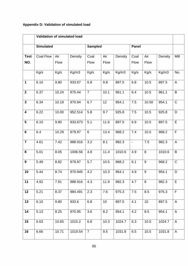
85
Appendix D: Validation of simulated load
Validation of simulated load
Simulated Sampled Panel
Test
NO.
Coal Flow Air
Flow
Density Coal
Flow
Air
Flow
Density Coal
Flow
Air
Flow
Density Mill
Kg/s Kg/s Kg/m3 Kg/s Kg/s Kg/m3 Kg/s Kg/s Kg/m3 No.
1 6.10 9.80 933.67 6.8 9.8 897.5 6.8 10.5 897.5 A
2 6.37 10.24 975.44 7 10.1 961.1 6.4 10.5 961.1 B
3 6.34 10.19 970.94 6.7 12 954.1 7.5 10.50 954.1 C
4 6.22 10.00 952.514 5.8 9.7 925.8 7.5 10.5 925.8 D
5 6.10 9.80 933.673 5.1 11.6 897.5 6.9 10.5 897.5 E
6 6.4 10.29 979.97 6 13.4 968.2 7.4 10.5 968.2 F
7 4.61 7.42 988.916 3.2 8.1 982.3 - 7.5 982.3 A
8 5.01 8.05 1006.56 4.8 11.4 1010.6 4.9 8 1010.6 B
9 5.49 8.82 979.97 5.7 10.5 968.2 6.1 9 968.2 C
10 5.44 8.74 970.945 4.2 10.3 954.1 4.9 9 954.1 D
11 4.92 7.91 988.916 4.3 11.9 982.3 4.7 8 982.3 E
12 5.21 8.37 984.491 2.3 7.6 975.3 7.5 8.5 975.3 F
13 6.10 9.80 933.6 6.8 10 897.5 4.1 10 897.5 A
14 5.13 8.25 970.95 3.6 8.2 954.1 4.2 8.5 954.1 A
15 6.63 10.65 1015.2 6.8 10.3 1024.7 6.3 10.5 1024.7 A
16 6.66 10.71 1019.54 7 9.5 1031.8 6.5 10.5 1031.8 A
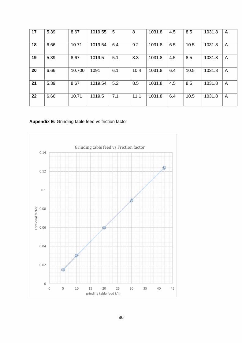
86
17 5.39 8.67 1019.55 5 8 1031.8 4.5 8.5 1031.8 A
18 6.66 10.71 1019.54 6.4 9.2 1031.8 6.5 10.5 1031.8 A
19 5.39 8.67 1019.5 5.1 8.3 1031.8 4.5 8.5 1031.8 A
20 6.66 10.700 1091 6.1 10.4 1031.8 6.4 10.5 1031.8 A
21 5.39 8.67 1019.54 5.2 8.5 1031.8 4.5 8.5 1031.8 A
22 6.66 10.71 1019.5 7.1 11.1 1031.8 6.4 10.5 1031.8 A
Appendix E: Grinding table feed vs friction factor
0
0.02
0.04
0.06
0.08
0.1
0.12
0.14
0 5 10 15 20 25 30 35 40 45
Fric
tio
nal
fac
tor
grinding table feed t/hr
Grinding table feed vs Friction factor
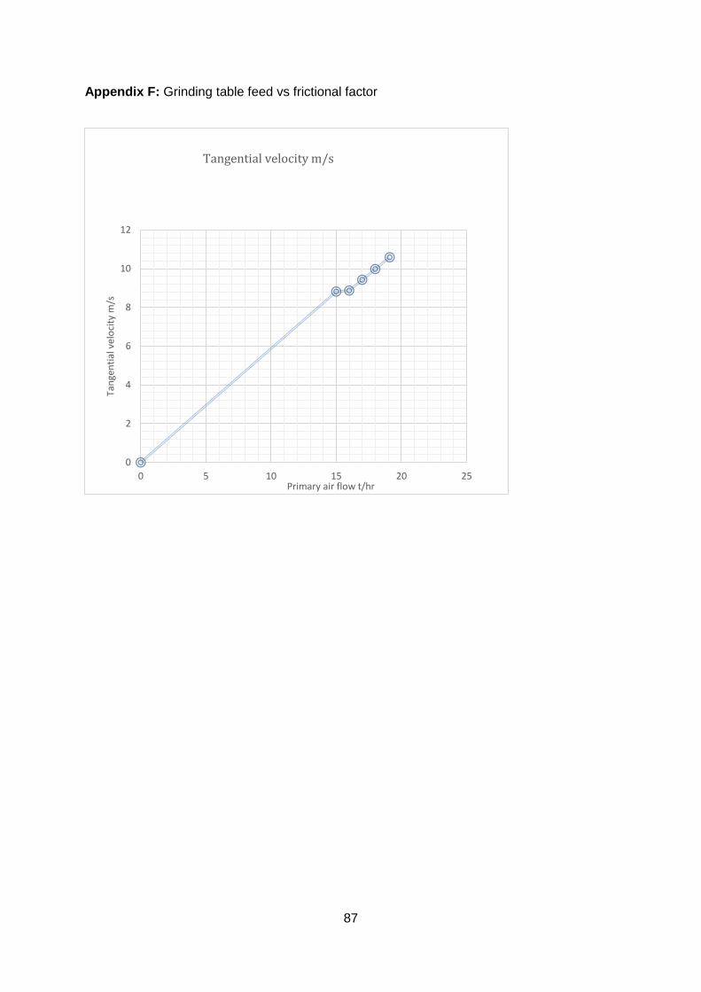
87
Appendix F: Grinding table feed vs frictional factor
0
2
4
6
8
10
12
0 5 10 15 20 25
Tan
gen
tial
vel
oci
ty m
/s
Primary air flow t/hr
Tangential velocity m/s
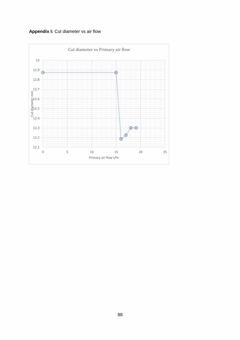
88
Appendix I: Cut diameter vs air flow
12.1
12.2
12.3
12.4
12.5
12.6
12.7
12.8
12.9
13
0 5 10 15 20 25
Cu
t d
iam
eter
mm
Primary air flow t/hr
Cut diameter vs Primary air flow
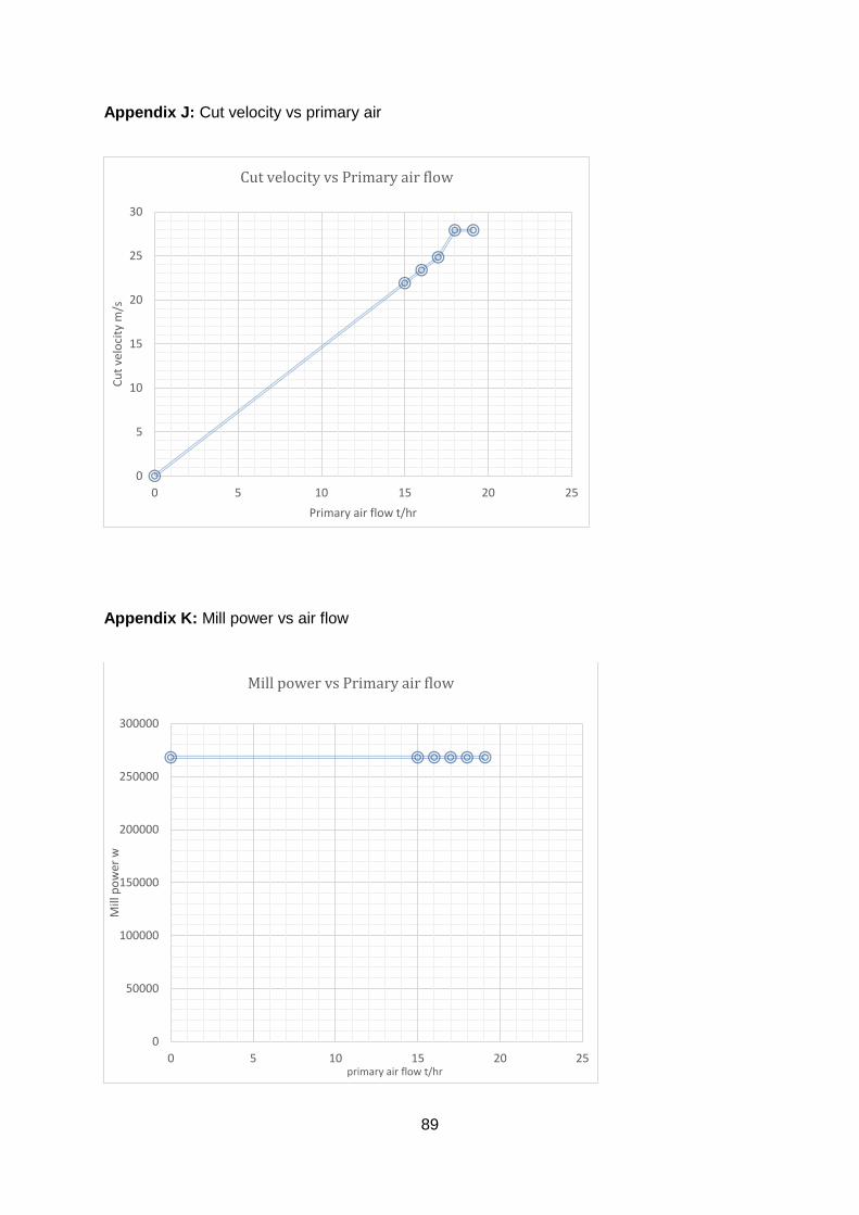
89
Appendix J: Cut velocity vs primary air
Appendix K: Mill power vs air flow
0
5
10
15
20
25
30
0 5 10 15 20 25
Cu
t ve
loci
ty m
/s
Primary air flow t/hr
Cut velocity vs Primary air flow
0
50000
100000
150000
200000
250000
300000
0 5 10 15 20 25
Mill
po
wer
w
primary air flow t/hr
Mill power vs Primary air flow
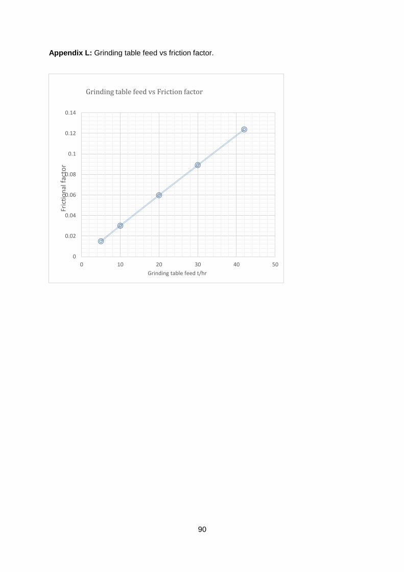
90
Appendix L: Grinding table feed vs friction factor.
0
0.02
0.04
0.06
0.08
0.1
0.12
0.14
0 10 20 30 40 50
Fric
tio
nal
fact
or
Grinding table feed t/hr
Grinding table feed vs Friction factor
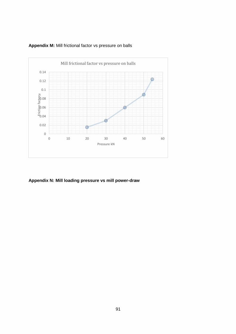
91
Appendix M: Mill frictional factor vs pressure on balls
Appendix N: Mill loading pressure vs mill power-draw
0
0.02
0.04
0.06
0.08
0.1
0.12
0.14
0 10 20 30 40 50 60
Fric
tio
n f
acto
rµ
Pressure kN
Mill frictional factor vs pressure on balls
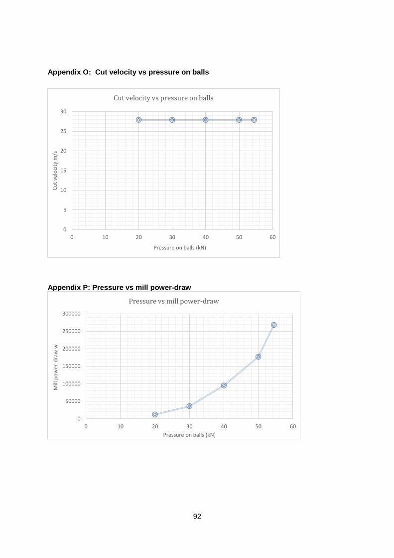
92
Appendix O: Cut velocity vs pressure on balls
Appendix P: Pressure vs mill power-draw
0
5
10
15
20
25
30
0 10 20 30 40 50 60
Cu
t ve
loci
ty m
/s
Pressure on balls (kN)
Cut velocity vs pressure on balls
0
50000
100000
150000
200000
250000
300000
0 10 20 30 40 50 60
Mill
po
wer
-dra
w w
Pressure on balls (kN)
Pressure vs mill power-draw
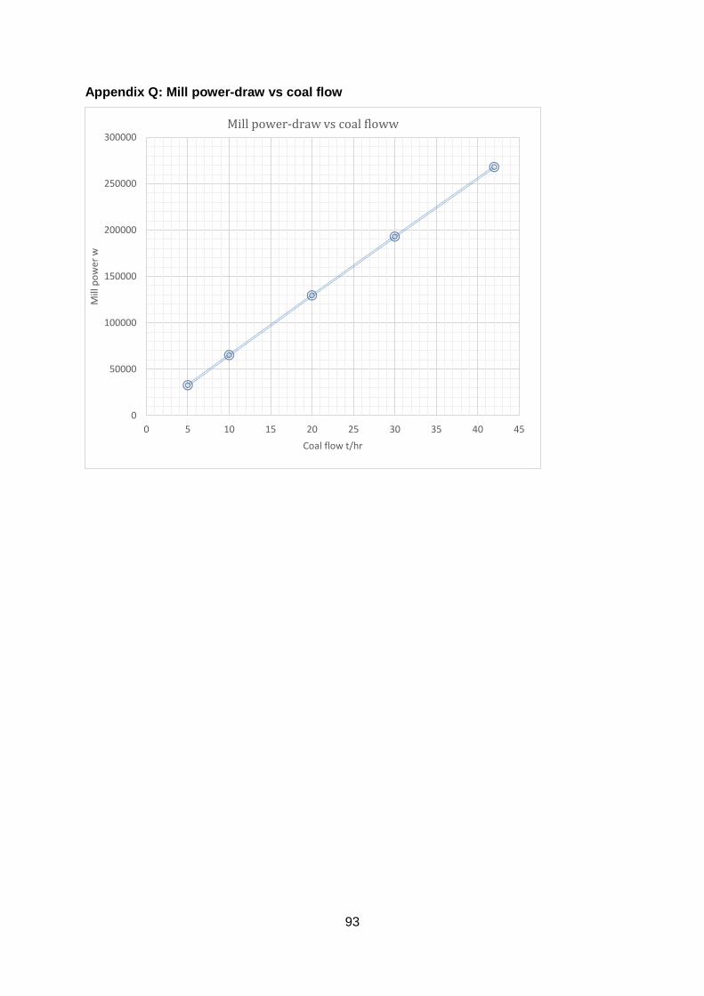
93
Appendix Q: Mill power-draw vs coal flow
0
50000
100000
150000
200000
250000
300000
0 5 10 15 20 25 30 35 40 45
Mill
po
wer
w
Coal flow t/hr
Mill power-draw vs coal floww
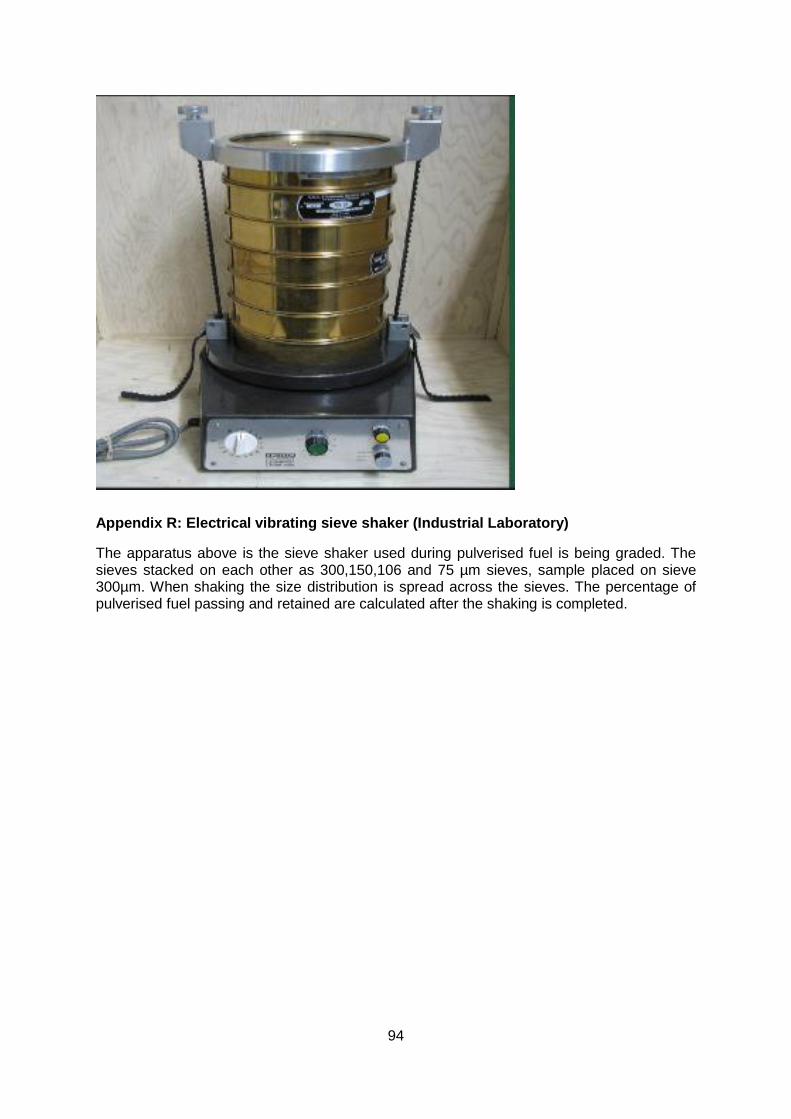
94
Appendix R: Electrical vibrating sieve shaker (Industrial Laboratory)
The apparatus above is the sieve shaker used during pulverised fuel is being graded. The sieves stacked on each other as 300,150,106 and 75 µm sieves, sample placed on sieve 300µm. When shaking the size distribution is spread across the sieves. The percentage of pulverised fuel passing and retained are calculated after the shaking is completed.
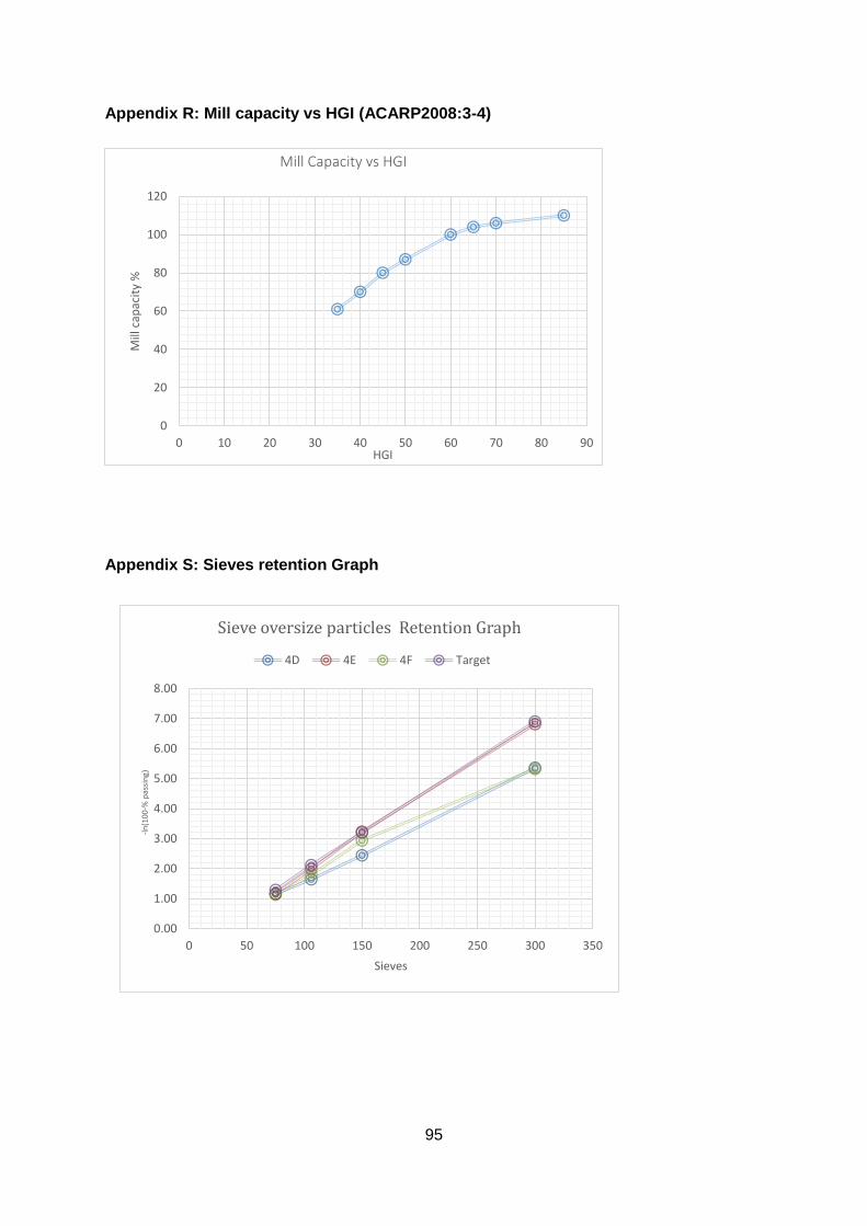
95
Appendix R: Mill capacity vs HGI (ACARP2008:3-4)
Appendix S: Sieves retention Graph
0
20
40
60
80
100
120
0 10 20 30 40 50 60 70 80 90
Mill
cap
acit
y %
HGI
Mill Capacity vs HGI
0.00
1.00
2.00
3.00
4.00
5.00
6.00
7.00
8.00
0 50 100 150 200 250 300 350
-ln
(100
-% p
assi
ng)
Sieves
Sieve oversize particles Retention Graph
4D 4E 4F Target
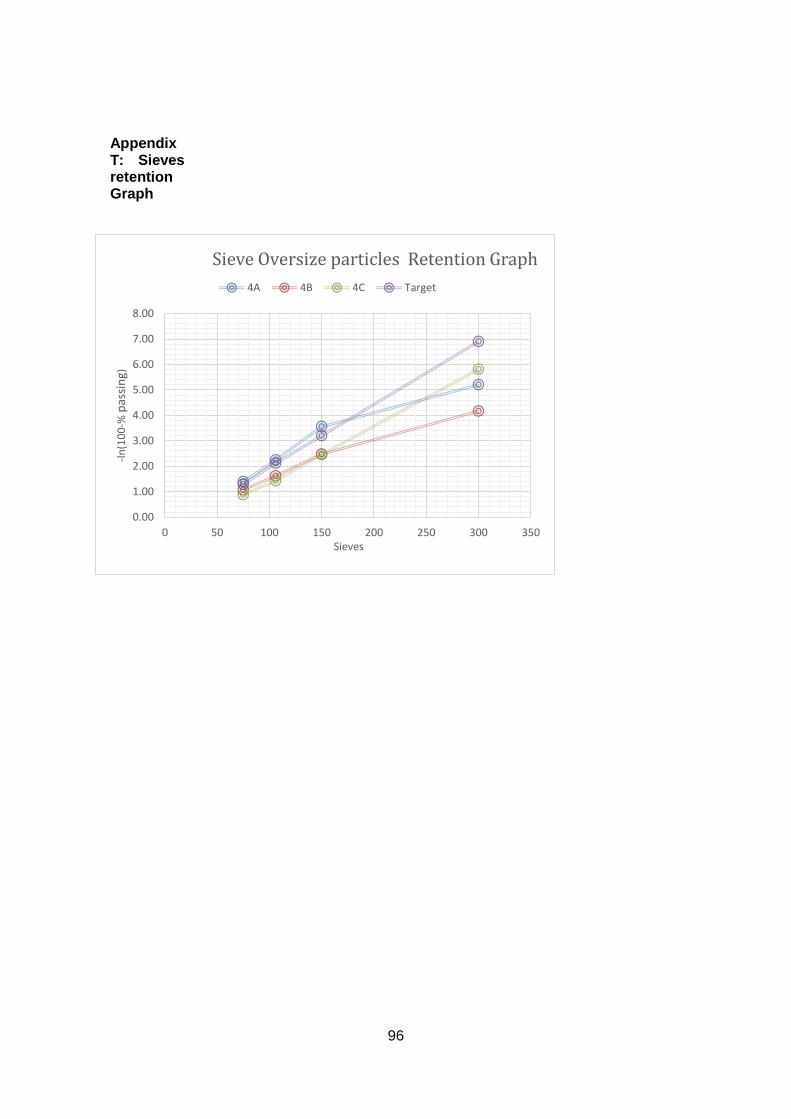
96
Appendix T: Sieves retention Graph
0.00
1.00
2.00
3.00
4.00
5.00
6.00
7.00
8.00
0 50 100 150 200 250 300 350
-ln
(10
0-%
pas
sin
g)
Sieves
Sieve Oversize particles Retention Graph
4A 4B 4C Target