Performance improvement of a high pressure steam turbine byoptimizing the exhaust geometry using CFD

Ch. Musch, S. Hecker, D. Gloss and R. Steinhoff

Siemens AG

Energy Sector

Rheinstr. 100

45478 Mulheim an der Ruhr, Germany

ABSTRACT

The design of modern steam turbines for power plant applications is steering for higher effi-

ciencies. A considerable contribution to this aim is expected from a reduction of flow losses in

turbine intakes and exhausts. The present study therefore deals with the optimization of the

exhaust of a high pressure (HP) turbine.

In the first part of this study a numerical model is presented which allows for a precise represen-

tation of the exhaust flow. This computational fluid dynamics (CFD) model has been validated

with a fair amount of experimental data from a test rig.

For the second part of the study comprehensive numerical investigations have been carried out,

considering the major geometrical parameters of such a geometry. In order to minimize the

effort in design time and preprocessing a fully parametric 3D model of the geometry is created

to prepare the different design variations. The results of these simulations allow to assess the

performance differences of given exhaust designs in the early design phase without the need for

expensive CFD simulations.

Finally the potential for improvement is shown by means of a comparison of an optimized design

to the baseline geometry.

NOMENCLATURE

kloss

[

1

m

]

Isotropic loss coefficient of porous region

pt [Pa] Total pressure

[

kg

m3

]

Density

c[

ms

]

Flow velocity

t [s] Time

d [m] Ring chamber diameter

R [−] Normalized span

ζ [−] Pressure loss coefficient of exhaust

AR [−] Area ratio

INTRODUCTION

Besides the effort to further increase the efficiency of modern steam turbine power plants the

design of the turbine is also driven by a demand to reduce costs. A major factor for the overall costs

of the turbine is the installation size of the turbine. Mostly a size reduction will be in conflict with

the reduction of flow losses. A more thorough look at the flow is therefore becoming more and more

essential to avoid unnecessary flow losses and efficiency penalties. The exhaust area of a turbine

is significant for the overall size of each turbine as the specific volume of the steam and hence the

volume of the flow passage increases from turbine inlet to outlet. By trying to reduce the size of the

1

Proceedings of

11th European Conference on Turbomachinery Fluid dynamics & Thermodynamics

ETC11, March 23-27, 2015, Madrid, Spain

OPEN ACCESS

Downloaded from www.euroturbo.eu Copyright © by the Authors

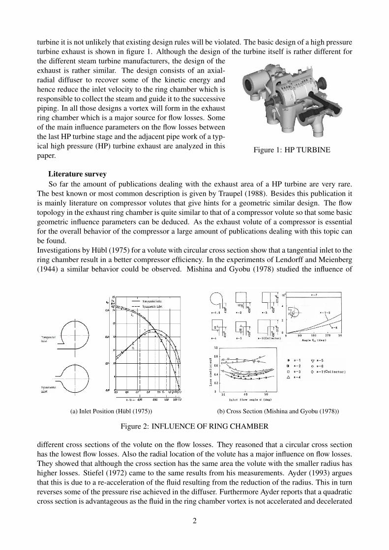
turbine it is not unlikely that existing design rules will be violated. The basic design of a high pressure

turbine exhaust is shown in figure 1. Although the design of the turbine itself is rather different for

Figure 1: HP TURBINE

the different steam turbine manufacturers, the design of the

exhaust is rather similar. The design consists of an axial-

radial diffuser to recover some of the kinetic energy and

hence reduce the inlet velocity to the ring chamber which is

responsible to collect the steam and guide it to the successive

piping. In all those designs a vortex will form in the exhaust

ring chamber which is a major source for flow losses. Some

of the main influence parameters on the flow losses between

the last HP turbine stage and the adjacent pipe work of a typ-

ical high pressure (HP) turbine exhaust are analyzed in this

paper.

Literature survey

So far the amount of publications dealing with the exhaust area of a HP turbine are very rare.

The best known or most common description is given by Traupel (1988). Besides this publication it

is mainly literature on compressor volutes that give hints for a geometric similar design. The flow

topology in the exhaust ring chamber is quite similar to that of a compressor volute so that some basic

geometric influence parameters can be deduced. As the exhaust volute of a compressor is essential

for the overall behavior of the compressor a large amount of publications dealing with this topic can

be found.

Investigations by Hubl (1975) for a volute with circular cross section show that a tangential inlet to the

ring chamber result in a better compressor efficiency. In the experiments of Lendorff and Meienberg

(1944) a similar behavior could be observed. Mishina and Gyobu (1978) studied the influence of

(a) Inlet Position (Hubl (1975)) (b) Cross Section (Mishina and Gyobu (1978))

Figure 2: INFLUENCE OF RING CHAMBER

different cross sections of the volute on the flow losses. They reasoned that a circular cross section

has the lowest flow losses. Also the radial location of the volute has a major influence on flow losses.

They showed that although the cross section has the same area the volute with the smaller radius has

higher losses. Stiefel (1972) came to the same results from his measurements. Ayder (1993) argues

that this is due to a re-acceleration of the fluid resulting from the reduction of the radius. This in turn

reverses some of the pressure rise achieved in the diffuser. Furthermore Ayder reports that a quadratic

cross section is advantageous as the fluid in the ring chamber vortex is not accelerated and decelerated

2

with every revolution. On the contrary Brown and Bradshaw (1949) performed measurements for four

double volutes with different cross-sectional shapes. They argue that neither the inlet position to the

volute nor the form of the cross section have a significant influence on the compressor performance.

However, Yang et al. (2011) analyzed four different types of cross-section shapes with symmetric

inlet and found a round shape to give the highest pump efficiency. Reunanen (2001) claims that the

shape of the cross section is of minor importance as the tangential velocity is much higher compared

to the radial velocity. This however may not be true for a turbine exhaust.

VALIDATION OF NUMERICAL MODEL

In this section a numerical model is presented which is validated with the help of test rig measure-

ments. In the first part the test rig will be introduced briefly and in the following sections the influence

of mesh size and turbulence modeling will be discussed.

Test Rig

Measurements were conducted by Urban (1997) in the late 1990’s. A scaled plexiglas model has

been investigated, which is similar to an actual HP turbine exhaust. Figure 3 shows a photography

Figure 3: TEST RIG (Urban (1997))

of the model. The geometry of the cross section as well as

the circumferential design are shown in figure 4. It can be

seen that the model features two exhaust ports and a con-

stant annular cross section around the circumference. Fur-

thermore the different measurement planes can be identified.

Pressure taps for static pressure measurements have been in-

stalled in the inlet of the test rig as well as in plane 0 and

plane 1. Plane 0 and plane 1 are the diffuser inlet and diffuser

outlet plane respectively. As can be seen in figure 4 measure-

ments have been conducted in these planes at eight different

positions around the circumference. Stagnation pressure has

been measured at the same locations and additionally in the

outlet flange to determine the overall flow losses. For this

purpose a five hole wedge type probe has been traversed

at these locations. Hence, beside the stagnation pressure

the complete velocity vector has been determined along the

channel span. The test rig has been driven by a compressor

and exhausts to ambient. A perforated metal sheet at the inlet has been used to model the upstream

turbine stages. Similar to a real turbine it creates a rather homogeneous mass flow and total pressure

Figure 4: TEST RIG GEOMETRY AND MEASUREMENT LOCATIONS (Urban (1997))

3

field around the circumference. This has further been accompanied by 24 flow guides in the inlet

section to suppress any tangential velocity field. The test rig could be equipped with different diffuser

designs. Two of these have been used for the validation. The first diffuser has a very moderate area

ratio of 1.2 showing no flow separation within the diffuser. The second one is a bit more aggressive

with an area ratio of 1.6 showing considerable flow separation.

Numerical Model Part 1

The numerical simulations carried out in this study are conducted with the commercial software

code ANSYS CFX. Steady state as well as transient simulations are done to determine the flow losses

for the different geometries. Spatial discretization is done using a high resolution scheme, resulting in

almost second order accuracy. For all transient simulations a temporal discretization using an implicit

second order Euler scheme is employed. Turbulence closure is done with an eddy viscosity approach

based on the Reynolds-Averaged Navier-Stokes equations. For the validation of the numerical model

different turbulence models have been investigated. Besides the turbulence models also the mesh size

is investigated. In order to allow for an automated grid generation, an unstructured tetrahedral mesh-

ing approach is used. Additional inflation layers (using prism elements) next to all solid walls are

utilized to accurately calculate the boundary layers. Figure 5 shows a typical mesh of the computa-

tional domain. Fluid properties have been modeled using an ideal gas assumption for the simulation

Figure 5: SYMMETRIC MESH OF TEST RIG MODEL

of the air driven test rig. The test rig is modeled starting upstream of the perforated metal sheet and

downstream to the exhaust ports. The perforated metal is modeled as a porous medium with a linear

loss characteristics. The loss coefficient is calculated according to equation 1 to reflect the measured

pressure loss.

kloss =∆pt,plate

b2c2

(1)

with b and c being the metal sheet width and the flow velocity, respectively. The pressure loss across

the metal sheet is roughly one order of magnitude higher than the losses of the exhaust itself. As a

boundary condition at the inlet the stagnation pressure and temperature are used. As outlet boundary

condition the mass flow is prescribed.

Mesh Sensitivity and Model Inaccuracy

In a first set of simulations the sensitivity towards mesh resolution is investigated. The k − ωturbulence model is used for the presented results. The global mesh size and the boundary layer

resolution are varied separately and the results are analyzed with regard to overall pressure loss. To

minimize the computational effort at this stage of the study it is thought to be reasonable to exploit the

symmetry of the model, i.e. only one half of the test rig is modeled in CFD. The results gained in this

study are shown in table 1. The loss coefficients are normalized with the value of mesh 4. Based on

4

Table 1: DATA OF MESH STUDY

Mesh 1 Mesh 2 Mesh 3 Mesh 4 Mesh 5 Mesh 6

Mesh size (Node Count) 4 mio 3 mio 3 mio 2.5 mio 2.5 mio 2 mio

Boundary Layer Resolution (y+max) 10.0 10.1 5.3 9.9 10.0 19.0

Number of Prism Layers 30 23 23 23 19 15

Normalized Loss Coefficient 0.976 0.988 1.008 1.000 0.984 0.869

this study a grid resolution according to the mesh parameters used in mesh 4 is found to be sufficient

for an accurate (below 3% difference to the finest investigated mesh) representation of the flow losses.

Figure 6: FLOW DIRECTIONS (1)

As a further proof the flow profiles gained from meshes 1

and 4 are compared to each other. Figures 7a and 7b show

the velocity profiles corresponding to measurement plane

1 (i.e. diffuser outlet) for positions 1 and 5. The defini-

tions of the flow directions, as used in the these plots, are

given in figure 6. These definitions will also be used later

on. Although some differences could be observed in the

flow profiles for the two meshes the discrepancy to the mea-

surements is even more noticeable. This of course can be

attributed to the symmetry boundary condition used in the

CFD, which constricts the flow in an unrealistic way. Consequently, a simulation using a full

model is carried out. However, due to the additional degree of freedom the flow becomes rather

0 0.2 0.4 0.6 0.8 1-20

0

20

40

60

Span [%]

Vel

ocity

[m

/s]

CFD, Mesh4-full

CFD, Mesh1-full

CFD, Mesh4-sym

CFD, Mesh1-sym

(a) Pos.1

0 0.2 0.4 0.6 0.8 1-20

0

20

40

60

Span [%]

Vel

ocity

[m

/s]

Radial Velocity

Circumferential Velocity

(b) Pos.5

Figure 7: VELOCITY PROFILES AT DIFFUSER OUTLET / MESH SENSITIVITY AND MODEL

ERRORS

10-1

100

101

0.6

0.7

0.8

0.9

1

1.1

CFLglobal [-]

ζ norm

[-]

Figure 8: INFLUENCE OF TIME STEP SIZE

unsteady in these regions and a converged

steady state solution is hard to find. Thus,

a transient simulation must be carried out to

correctly predict the whole flow field. In or-

der to minimize the computational effort it

is first of all investigated how the time step

of the simulation influences the results. Pri-

marily this is done in order to determine the

largest possible time step. To be able to trans-

fer the results to other geometries a global

Courant number is introduced. In equation 2,

variables d,c and ∆t denote the ring chamber

5

diameter, the average flow velocity and the actual time step of the simulation.

CFLglobal =c ·∆t

d(2)

From figure 8 it can be seen that up to a value of CFLglobal = 0.2 there is hardly any change to the

calculated pressure losses. The corresponding time step will thus be used further on. Also all further

simulations described in section PARAMETER STUDY are done accordingly.

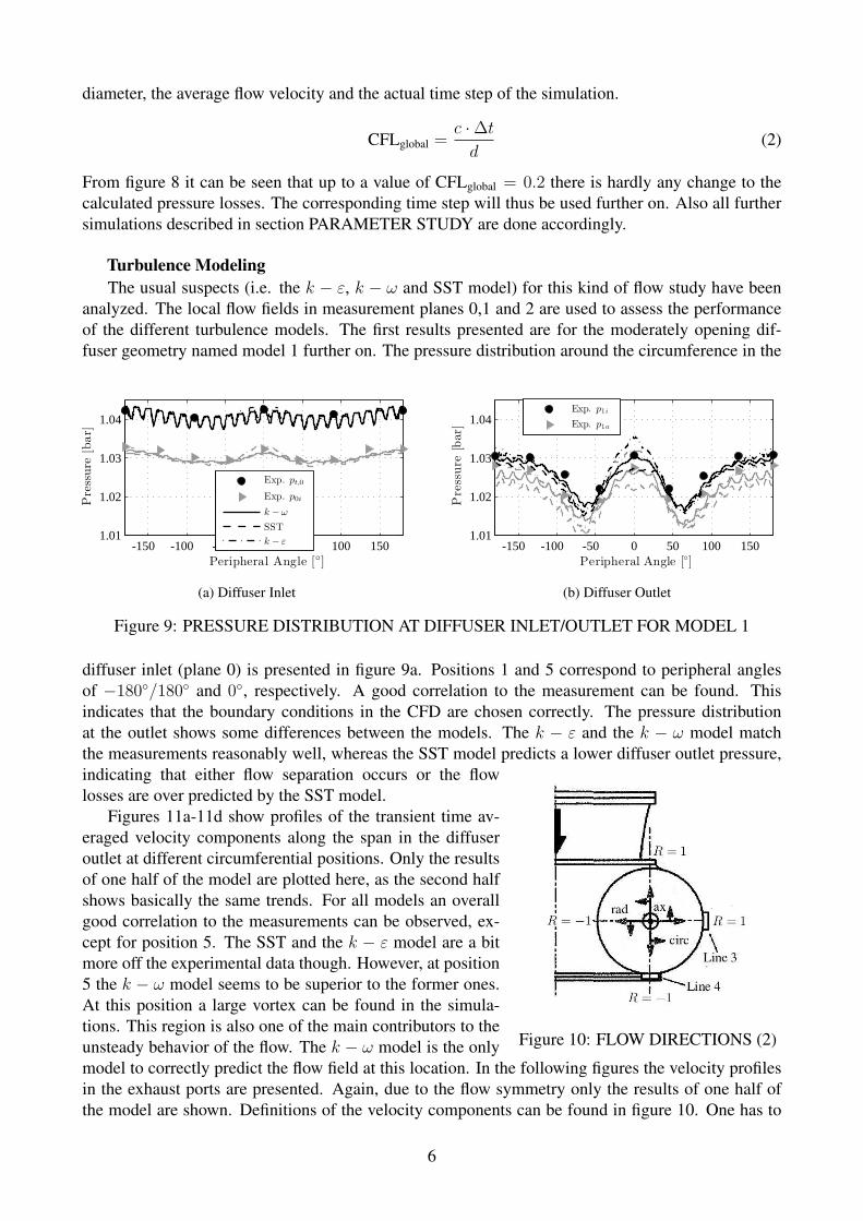
Turbulence Modeling

The usual suspects (i.e. the k − ε, k − ω and SST model) for this kind of flow study have been

analyzed. The local flow fields in measurement planes 0,1 and 2 are used to assess the performance

of the different turbulence models. The first results presented are for the moderately opening dif-

fuser geometry named model 1 further on. The pressure distribution around the circumference in the

-150 -100 -50 0 50 100 1501.01

1.02

1.03

1.04

Peripheral Angle [◦]

Pre

ssure

[bar]

Exp. pt,0

Exp. p0i

k −ω

SST

k − ε

(a) Diffuser Inlet

-150 -100 -50 0 50 100 1501.01

1.02

1.03

1.04

Peripheral Angle [◦]

Pressure

[bar]

Exp. p1i

Exp. p1a

(b) Diffuser Outlet

Figure 9: PRESSURE DISTRIBUTION AT DIFFUSER INLET/OUTLET FOR MODEL 1

diffuser inlet (plane 0) is presented in figure 9a. Positions 1 and 5 correspond to peripheral angles

of −180◦/180◦ and 0◦, respectively. A good correlation to the measurement can be found. This

indicates that the boundary conditions in the CFD are chosen correctly. The pressure distribution

at the outlet shows some differences between the models. The k − ε and the k − ω model match

the measurements reasonably well, whereas the SST model predicts a lower diffuser outlet pressure,

Figure 10: FLOW DIRECTIONS (2)

indicating that either flow separation occurs or the flow

losses are over predicted by the SST model.

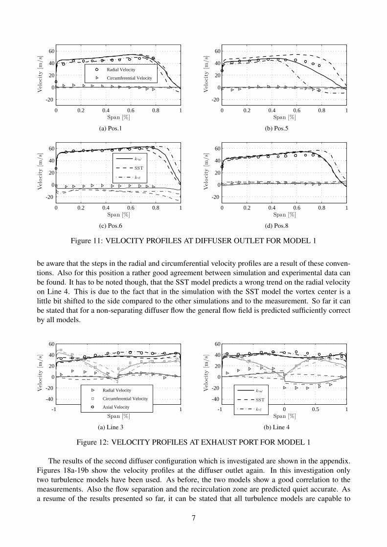
Figures 11a-11d show profiles of the transient time av-

eraged velocity components along the span in the diffuser

outlet at different circumferential positions. Only the results

of one half of the model are plotted here, as the second half

shows basically the same trends. For all models an overall

good correlation to the measurements can be observed, ex-

cept for position 5. The SST and the k − ε model are a bit

more off the experimental data though. However, at position

5 the k − ω model seems to be superior to the former ones.

At this position a large vortex can be found in the simula-

tions. This region is also one of the main contributors to the

unsteady behavior of the flow. The k − ω model is the only

model to correctly predict the flow field at this location. In the following figures the velocity profiles

in the exhaust ports are presented. Again, due to the flow symmetry only the results of one half of

the model are shown. Definitions of the velocity components can be found in figure 10. One has to

6

0 0.2 0.4 0.6 0.8 1

-20

0

20

40

60

Span [%]

Vel

oci

ty[m

/s]

Radial Velocity

Circumferential Velocity

(a) Pos.1

0 0.2 0.4 0.6 0.8 1

-20

0

20

40

60

Span [%]

Vel

oci

ty[m

/s]

(b) Pos.5

0 0.2 0.4 0.6 0.8 1

-20

0

20

40

60

Span [%]

Vel

oci

ty[m

/s]

k-ω

SST

k-ε

(c) Pos.6

0 0.2 0.4 0.6 0.8 1

-20

0

20

40

60

Span [%]

Vel

oci

ty[m

/s]

(d) Pos.8

Figure 11: VELOCITY PROFILES AT DIFFUSER OUTLET FOR MODEL 1

be aware that the steps in the radial and circumferential velocity profiles are a result of these conven-

tions. Also for this position a rather good agreement between simulation and experimental data can

be found. It has to be noted though, that the SST model predicts a wrong trend on the radial velocity

on Line 4. This is due to the fact that in the simulation with the SST model the vortex center is a

little bit shifted to the side compared to the other simulations and to the measurement. So far it can

be stated that for a non-separating diffuser flow the general flow field is predicted sufficiently correct

by all models.

-1 -0.5 0 0.5 1

-40

-20

0

20

40

60

Span [%]

Vel

oci

ty[m

/s]

Radial Velocity

Circumferential Velocity

Axial Velocity

(a) Line 3

-1 -0.5 0 0.5 1

-40

-20

0

20

40

60

Span [%]

Vel

oci

ty[m

/s]

k-ω

SST

k-ε

(b) Line 4

Figure 12: VELOCITY PROFILES AT EXHAUST PORT FOR MODEL 1

The results of the second diffuser configuration which is investigated are shown in the appendix.

Figures 18a-19b show the velocity profiles at the diffuser outlet again. In this investigation only

two turbulence models have been used. As before, the two models show a good correlation to the

measurements. Also the flow separation and the recirculation zone are predicted quiet accurate. As

a resume of the results presented so far, it can be stated that all turbulence models are capable to

7

predict the time average flow field good enough for the purposes of this paper. Ultimately, the k − ωmodel is chosen for all further investigations as it showed slightly better results in comparison to the

experiments.

PARAMETER STUDY

For this part of the paper a parametric model of the exhaust has been created. The geometry is a

generic model of a typical barrel type HP turbine. Parameters which have been investigated are the

aspect ratio of the exhaust ring chamber cross-section, the corner radii of the chamber and the wall

angles. The influence of all these parameters on the overall pressure loss ∆pt is evaluated by means

of a normalized pressure loss coefficient, which yields the definition for ζnorm shown in equation 3.

ζnorm =∆pt

∆pt,baseline

(3)

Figure 13 shows a 3D model of the exhaust with the stator vane and rotor blades as well as the

parameters of the ring chamber cross section. The ring chamber has a constant cross section between

sections 6-7-8-1-2-3-4 (as defined in figure 4). The baseline design which is shown in figure 13 in the

3D view is furthermore characterized by a quadratic cross section with 90◦ wall angles. The corner

Figure 13: NUMERICAL SETUP FOR PARAMETER STUDY

radii have a size of R = 80mm and the area of the constant part of the ring chamber as shown in

figure 13 is defined by a ratio of AR = 0.75 with reference to the exhaust port area.

Numerical Model Part 2

In order to correctly predict the flow losses it is important that the flow entering the exhaust

chamber is as close as possible to the actual inflow conditions of the turbine. This is ensured in

the present study by including the last stator and rotor row of the turbine in the CFD model. As the

exhaust geometry is not symmetric around the circumference, also the flow field will vary accordingly.

To account for that, all blades of the last rotor row are modeled. The stator vane and the rotor blade

are connected via a Mixing-Plane- (or Stage-) Interface. The rotor domain is connected to the exhaust

domain using a transient rotor-stator (or sliding mesh) interface. As inlet boundary conditions the

mass flow and total temperature are applied. At the outlet, the static pressure is prescribed. Fluid

properties are taken from a steam table according to IAPWS-IF97. Although the mesh of the blade

and vane are chosen to be very coarse the overall node count adds up to roughly 7.5 Mio. nodes.

8

Corner Radii

In the first part of the study the influence of the corner radii on the flow field is investigated.

Therefore, four different radii are analyzed with an otherwise unchanged geometry. It can be shown

that the flow losses are increasing as the radius is increased. This can be explained when taking a look

at the flow field in the ring chamber. Figure 14 shows the tangential velocity and the corresponding

pressure field normalized by the inlet pressure in a horizontal cut plane (see figure 13) for the investi-

gated geometries. It can be seen that with a larger radius also the flow velocity gets higher. Due to the

higher flow velocity it is apparent that the losses are likewise increasing. This however can be further

explained from the contour plots of the pressure at the corresponding position. In these contour plots

the pressure can be found to be high in the corners of the chamber as a result of flow stagnation in the

corners. This pressure increase leads to a decrease of the rotational velocity of the vortex and thus to

a decrease of friction losses. This is indeed a known feature from labyrinth seals. Kuwamura et al.

(2013) for example showed that a stepped labyrinth seal with a circular shaped cavity has a smaller

leakage flow than a rectangular shaped cavity due to an enhanced vortex velocity. Furthermore it can

be seen that an asymptotic behavior exists. Once the radius goes below a certain value the pressure

field does not change markedly and thus also the losses are almost constant. The baseline design

therefore already has a reasonable size with respect to aerodynamic considerations.

Figure 14: VELOCITY AND PRESSURE FIELD FOR DIFFERENT CORNER RADII

Wall Angles

The next parameters investigated are the wall angles a1 and a2. Figure 15 shows the flow fields of

four different geometries, which have been simulated. Angles of 75◦ and 105◦ have been considered

in the CFD for both sides. The influence of angle a1 on the overall pressure loss is hardly visible.

Accordingly, only a minor influence on the rotational velocity can be determined as shown in figure

Figure 15: VELOCITY AND PRESSURE FIELD FOR DIFFERENT WALL ANGLES

15. It can thus be deduced that the drag forces in the corners are not markedly raised by changing

wall angle a1. However, by changing angle a2 a reasonable change in the pressure losses can be

identified. For an angle of a2 = 105◦ a slight reduction of the overall losses can be observed. From

the pressure plot shown in figure 15 for this configuration a steeper pressure rise along the angled

wall is perceptible when compared to the baseline design in figure 14. This can be attributed to an

9

additional diffusion due to the inclined wall. Also the size of the ring vortex is reduced in this setup

which as well contributes to the decreased losses. Taking a look at the configuration with a2 = 75◦ an

opposing effect can be seen, which is even more prominent. In this case the flow is accelerated rather

than decelerated resulting in a higher rotational velocity and therefore a higher pressure loss. A bent

in this direction should therefore be avoided if possible.

Aspect Ratio

The next parameter that is varied is the aspect ratio of the ring chamber. In all seven different

configurations have been investigated. The flow field in the horizontal cut plane is again used to

visualize the flow topology. Figure 16 shows the results for those simulations. As apparent from

the rotational velocity of the chamber vortex, in general the flow losses decrease from small to large

aspect ratio. Taking a closer look at the different results it can be seen that for very large aspect ratios

an additional counter-rotating ring vortex is formed,resulting in two smaller vortices. This reduces the

losses furthermore as on the one hand the lower vortex (with high rotational velocity) is small and thus

the losses attributed to this vortex are likewise small. On the other hand the upper vortex has a very

low rotational velocity due to a strong diffusion of the flow field between both vortices. In general

a larger chamber radius is advantageous due to additional flow deceleration caused by an increased

flow area resulting from the larger radius. This has also been pointed out by Steglich et al. (2008) in

their study on different compressor volutes. For small aspect ratios the formation of a second vortex

can hardly be found. Only for the smallest aspect ratio considered in this study a very small counter-

rotating vortex can be identified. For this configuration indeed the rotational velocity of the vortices

is indeed reduced compared to the case with h/w = 0.6. However, the overall losses are still on the

same level as the flow losses created in the transition from the ring chamber to the exhaust port are

increasing with smaller aspect ratios.

Figure 16: VELOCITY AND PRESSURE FIELD FOR DIFFERENT ASPECT RATIOS

Optimized Design

Finally, a combination of the design features formerly analyzed is investigated. Thus, a configura-

tion with corner radii of R = 80mm, an aspect ratio of h/w = 2 and inclined sidewalls with angles of

10

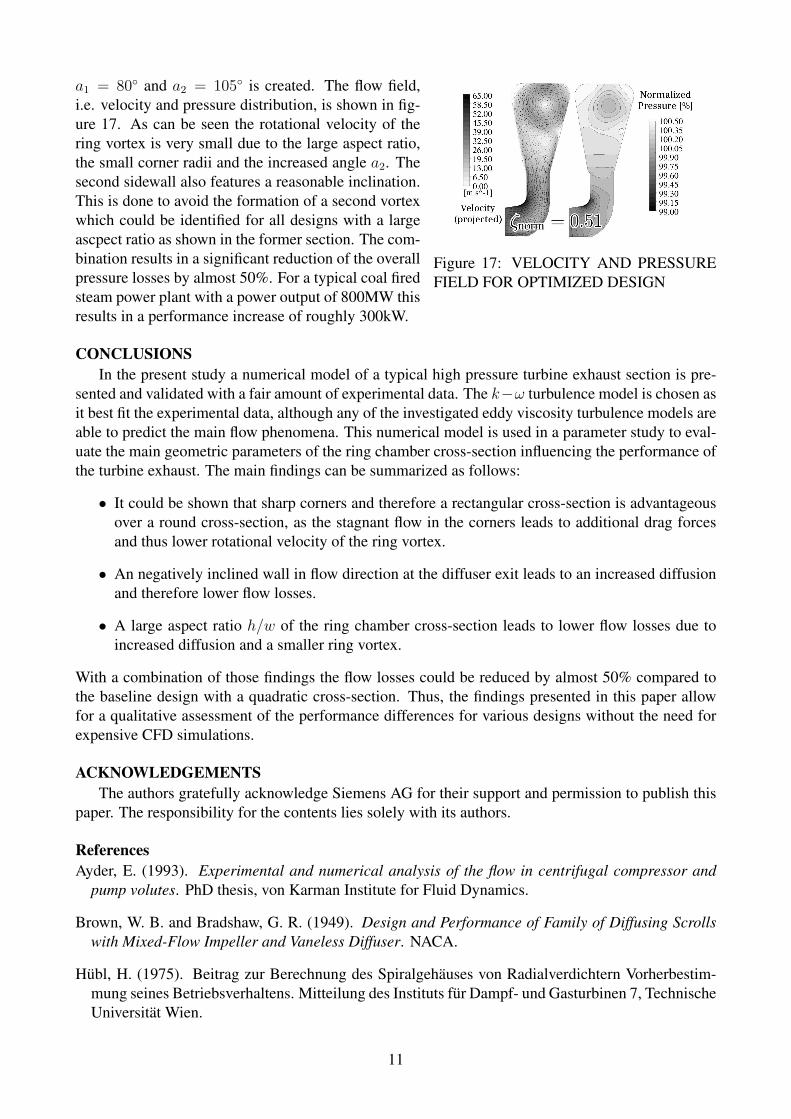
Figure 17: VELOCITY AND PRESSURE

FIELD FOR OPTIMIZED DESIGN

a1 = 80◦ and a2 = 105◦ is created. The flow field,

i.e. velocity and pressure distribution, is shown in fig-

ure 17. As can be seen the rotational velocity of the

ring vortex is very small due to the large aspect ratio,

the small corner radii and the increased angle a2. The

second sidewall also features a reasonable inclination.

This is done to avoid the formation of a second vortex

which could be identified for all designs with a large

ascpect ratio as shown in the former section. The com-

bination results in a significant reduction of the overall

pressure losses by almost 50%. For a typical coal fired

steam power plant with a power output of 800MW this

results in a performance increase of roughly 300kW.

CONCLUSIONS

In the present study a numerical model of a typical high pressure turbine exhaust section is pre-

sented and validated with a fair amount of experimental data. The k−ω turbulence model is chosen as

it best fit the experimental data, although any of the investigated eddy viscosity turbulence models are

able to predict the main flow phenomena. This numerical model is used in a parameter study to eval-

uate the main geometric parameters of the ring chamber cross-section influencing the performance of

the turbine exhaust. The main findings can be summarized as follows:

• It could be shown that sharp corners and therefore a rectangular cross-section is advantageous

over a round cross-section, as the stagnant flow in the corners leads to additional drag forces

and thus lower rotational velocity of the ring vortex.

• An negatively inclined wall in flow direction at the diffuser exit leads to an increased diffusion

and therefore lower flow losses.

• A large aspect ratio h/w of the ring chamber cross-section leads to lower flow losses due to

increased diffusion and a smaller ring vortex.

With a combination of those findings the flow losses could be reduced by almost 50% compared to

the baseline design with a quadratic cross-section. Thus, the findings presented in this paper allow

for a qualitative assessment of the performance differences for various designs without the need for

expensive CFD simulations.

ACKNOWLEDGEMENTS

The authors gratefully acknowledge Siemens AG for their support and permission to publish this

paper. The responsibility for the contents lies solely with its authors.

References

Ayder, E. (1993). Experimental and numerical analysis of the flow in centrifugal compressor and

pump volutes. PhD thesis, von Karman Institute for Fluid Dynamics.

Brown, W. B. and Bradshaw, G. R. (1949). Design and Performance of Family of Diffusing Scrolls

with Mixed-Flow Impeller and Vaneless Diffuser. NACA.

Hubl, H. (1975). Beitrag zur Berechnung des Spiralgehauses von Radialverdichtern Vorherbestim-

mung seines Betriebsverhaltens. Mitteilung des Instituts fur Dampf- und Gasturbinen 7, Technische

Universitat Wien.

11

Kim, S., Park, J., Ahn, K., and Baek, J. (2010). Improvement of the performance of a centrifugal

compressor by modifying the volute inlet. Journal of Fluids Engineering, 132(9).

Kuwamura, Y., Matsumoto, K., and Uehara, H. (2013). Development of new high-performance

labyrinth seal using aerodynamic approach. In Proceedings of ASME Turbo Expo. GT2013-94106.

Lendorff, B. and Meienberg, H. (1944). Detail-Entwicklung im Bau von Turboverdichtern. Escher

Wyss Mitteilungen 7.

Mishina, H. and Gyobu, I. (1978). Performance investigations of large capacity centrifugal compres-

sors. In Proceedings of ASME. 78-GT-3.

Reunanen, A. (2001). Experimental and numerical analysis of different volutes in a centrifugal com-

pressor. PhD thesis, University of Technology Lappeenranta.

Steglich, T., Kitzinger, J., Seume, J., den Braembusche, R. V., and Prinsier, J. (2008). Improved

diffuser/volute combinations for centrifugal compressors. Journal of Turbomachinery, 130(1).

Stiefel, W. (1972). Experiences in the development of radial compressors. Lecture Series 50: Ad-

vanced Radial Compressors. von Karman.

Traupel, W. (1988). Thermische Turbomaschinen. Springer-Verlag, 3rd edition.

Urban, M. (1997). Experimentelle Stromungsuntersuchungen an Modellen von HD-Abstrom-

gehausen. Siemens Internal Report.

Yang, S., Kong, F., , and Chen, B. (2011). Research on pump volute design method using CFD.

International Journal of Rotating Machinery, 2011.

12

APPENDIX

0 0.2 0.4 0.6 0.8 1-20

0

20

40

60

Span [%]

Vel

ocity

[m

/s]

Radial Velocity

Circumferential Velocity

(a) Pos.1

0 0.2 0.4 0.6 0.8 1-20

0

20

40

60

Span [%]

Vel

ocity

[m

/s]

k-ω

SST

(b) Pos.5

0 0.2 0.4 0.6 0.8 1-50

0

50

100

Span [%]

Vel

ocity

[m

/s]

(c) Pos.6

0 0.2 0.4 0.6 0.8 1-20

0

20

40

60

Span [%]

Vel

ocity

[m

/s]

(d) Pos.8

Figure 18: VELOCITY PROFILES AT DIFFUSER OUTLET FOR MODEL 2

-1 -0.5 0 0.5 1

-40

-20

0

20

40

60

Span [%]

Vel

oci

ty[m

/s]

Radial Velocity

Circumferential Velocity

Axial Velocity

(a) Line 3

-1 -0.5 0 0.5 1

-40

-20

0

20

40

60

Span [%]

Vel

oci

ty[m

/s]

k-ω

SST

(b) Line 4

Figure 19: VELOCITY PROFILES AT EXHAUST PORT FOR MODEL 2

13