numerical loss prediction of high pressure steam turbine ... · numerical loss prediction of high...
TRANSCRIPT

Numerical Loss Prediction of High Pressure Steam Turbine Rotor
Airfoils
Bonaventure Ryan Nunes
Thesis Submitted to the faculty of
Virginia Polytechnic Institute and State University
in partial fulfillment of the requirements for the degree of
Master of Science
in
Aerospace Engineering
Co-Chairs
Srinath V. Ekkad & Wing F. Ng
Todd Lowe & Lin Ma
August 30th 2013, Blacksburg VA
Keywords : Steam, Turbines, Transonic Cascade, Aerodynamics, Pressure Loss, Computational
Fluid Dynamics (CFD), Ansys CFX

Abstract
Numerical Loss Prediction of High Pressure Steam Turbine Rotor Airfoils
Bonaventure Ryan Nunes
Steam turbines are widely used in various industrial applications, primarily for power extraction.
However, deviation for operating design conditions is a frequent occurrence for such machines,
and therefore, understanding their performance at off design conditions is critical to ensure that
the needs of the power demanding systems are met as well as ensuring safe operation of the steam
turbines. In this thesis, the aerodynamic performance of three different turbine airfoil sections (
baseline, mid radius and tip profile) as a function of angle of incidence and exit Mach numbers, is
numerically computed at 0.3 axial chords downstream of the trailing edge. It was found that the
average loss coefficient was low, owing to the fact that the flow over the airfoils was well behaved.
The loss coefficient also showed a slight decrease with exit Mach number for all three profiles.
The mid radius and tip profiles showed near identical performance due to similarity in their
geometries. It was also found out that the baseline profile showed a trend of substantial increase
in losses at positive incidences, due to the development of an adverse pressure zone on the blade
suction side surface. The mid radius profile showed high insensitivity to angle of incidence as well
as low exit flow angle deviation in comparison to the baseline blade.

iii
To my family & friends

iv
Acknowledgments
I would like to start out by first thanking my parents, Anthony and Irene Nunes for supporting me
both emotionally and financially throughout my academic career. I couldn’t have made it this far
without their grace and blessings. Having said this, I would like to thank my advisors Dr. Ekkad
and Dr. Ng for giving me an opportunity to work on this project as well as offering me sound
advice on my short comings. I would also like to thank Diganta Narzary and Nikhil Rao from
Elliot Turbo for their funding and valuable suggestions throughout the duration of this project.
I am very grateful to all my friends here at Virginia Tech. I couldn’t have made it through the last
two years without your company and support. I would like to thank my lab mates in particular,
Arnab Roy, Dorian Blot, Hunter Guilliams, Shreyas Srinivasan, Sakshi Jain, Jaideep Pandit,
Sridharan Ramesh, Xue Song. Special mentions go to Shreyas Srinivasan, Deepu Dilip, David
Gomez, Dorion Blot and Vivek Kumar for their suggestions in general as well as the fun times we
spent together belaboring on various topics. I would also like to mention my roommate Feras Rabie
and my friend Shunxi Ji, for offering me important suggestions during the initial days of my
graduate tenure.
On a closing note, I would like to thank both the mechanical and aerospace engineering
departments at Virginia tech for giving me an opportunity to finish my Master of Science in
engineering.

v
Table of Contents
Abstract ........................................................................................................................................... ii
Acknowledgments.......................................................................................................................... iv
Table of Contents ............................................................................................................................ v
List of Figures .............................................................................................................................. viii
List of Tables ................................................................................................................................. xii
Nomenclature ............................................................................................................................... xiii
1 Background & Introduction .................................................................................................... 1
1.1 Mechanism of Losses ....................................................................................................... 2
1.2 Loss Definition ................................................................................................................. 3
1.3 Literature Survey .............................................................................................................. 5
2 Geometry Preparation and Modeling .................................................................................... 10
2.1 Overview ........................................................................................................................ 10
2.2 Blade Geometries ............................................................................................................11
2.3 Fluid Domain and Geometry Set Up .............................................................................. 15
2.4 Mesh Generation and Metrics ........................................................................................ 16
2.4.1 Mesh Metrics .......................................................................................................... 20
2.4.2 Discussion of Mesh Metrics.................................................................................... 23

vi
2.5 CFD Solver & Theory .................................................................................................... 25
2.5.1 Boundary Conditions .............................................................................................. 26
2.5.2 Turbulence Modeling .............................................................................................. 28
3 Results and Discussion ......................................................................................................... 30
3.1 Test Matrix ..................................................................................................................... 30
3.2 Mesh Independence Study ............................................................................................. 32
3.3 Profile 1 (Baseline)......................................................................................................... 34
3.3.1 Blade Loading ......................................................................................................... 34
3.3.2 Variation of Loss Coefficient with Exit Mach Number .......................................... 42
3.3.3 Variation of Loss Coefficient with Incidence ......................................................... 45
3.4 Profile 2 (Mid Radius Section)....................................................................................... 49
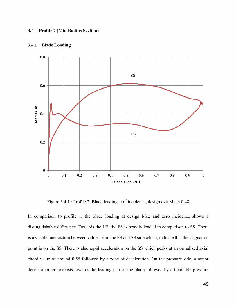
3.4.1 Blade Loading ......................................................................................................... 49
3.4.2 Variation of Loss Coefficient vs. Exit Mach Number ............................................. 56
3.4.3 Variation of Loss vs. Incidence ............................................................................... 58
3.5 Comparison between Profile 1 & Profile 2 .................................................................... 62
3.6 Comparison with Existing Literature ............................................................................. 67
3.7 Conclusions & Future Work ........................................................................................... 70
4 References ............................................................................................................................. 71
5 Appendix ............................................................................................................................... 73
5.1 Profile 1 Mesh Images.................................................................................................... 73

vii
5.2 Profile 4 Mesh and Loss Data ........................................................................................ 76

viii
List of Figures
Figure 2.2.1: Baseline Profile ........................................................................................................11
Figure 2.2.2 : Blade 2 (Pitch line profile) ..................................................................................... 12
Figure 2.2.3 : Blade 3 (Tip profile) ............................................................................................... 12
Figure 2.2.4 : Blade Nomenclature (a) .......................................................................................... 13
Figure 2.2.5 : Blade Nomenclature (b) ......................................................................................... 13
Figure 2.3.1 : Geometry of Profile 2 Passage ............................................................................... 15
Figure 2.4.1 : Profile 2 Mesh ........................................................................................................ 17
Figure 2.4.2 : O-grid mesh structure around the leading edge for Profile 2 ................................. 18
Figure 2.4.3 : O-grid mesh structure around the trailing edge for Profile 2 ................................. 18
Figure 2.4.4 : Mesh density within the wake region for Profile 2 ................................................ 19
Figure 2.4.5: Profile 2, LE Equiangular Skewness ....................................................................... 21
Figure 2.4.6 : Profile 2, TE Equiangular Skewness ...................................................................... 22
Figure 2.4.7 : Profile 2, Region of high Skew .............................................................................. 22
Figure 2.4.8 : Profile 2, Region of high aspect ratio ..................................................................... 23
Figure 2.5.1 : Sample of one side of symmetry boundary condition (marked in green) .............. 28
Figure 2.5.2 : SST model formulation [12] ................................................................................... 29
Figure 3.2.1 Profile 2: Dense unstructured Cells in the wake region ........................................... 33
Figure 3.3.1 : Profile 1 Blade loading at 0 incidence, design exit Mach 0.48 .............................. 34
Figure 3.3.2 : Profile 1, Pt variation across the blade at 0° incidence, Mex 0.48 ......................... 35
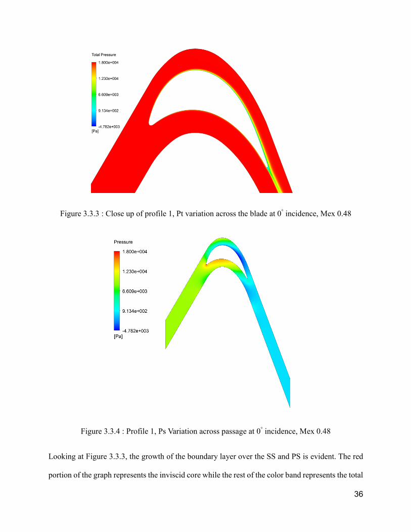
Figure 3.3.3 : Close up of profile 1, Pt variation across the blade at 0° incidence, Mex 0.48 ...... 36
Figure 3.3.4 : Profile 1, Ps Variation across passage at 0° incidence, Mex 0.48 ........................... 36
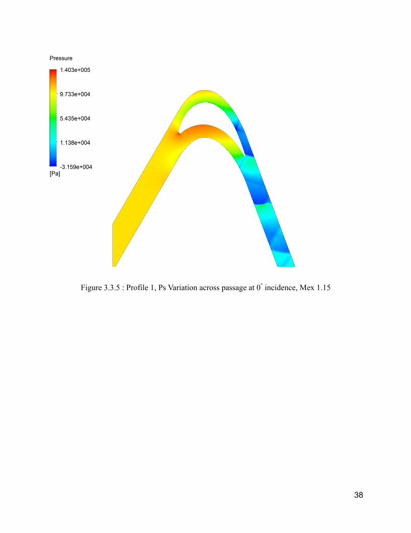
Figure 3.3.5 : Profile 1, Ps Variation across passage at 0° incidence, Mex 1.15 ........................... 38

ix
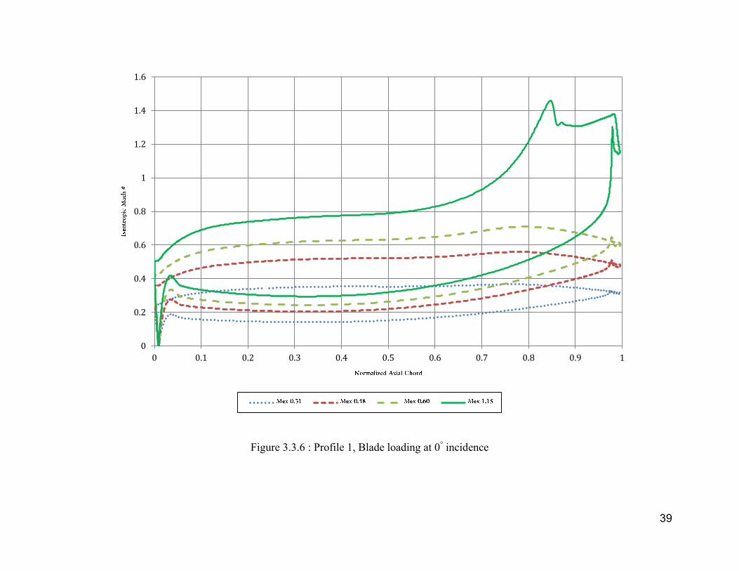
Figure 3.3.6 : Profile 1, Blade loading at 0° incidence ................................................................. 39
Figure 3.3.7 : Profile 1, Blade loading at +3° incidence ............................................................... 40
Figure 3.3.8 : Profile 1, Blade loading at +6° incidence ............................................................... 40
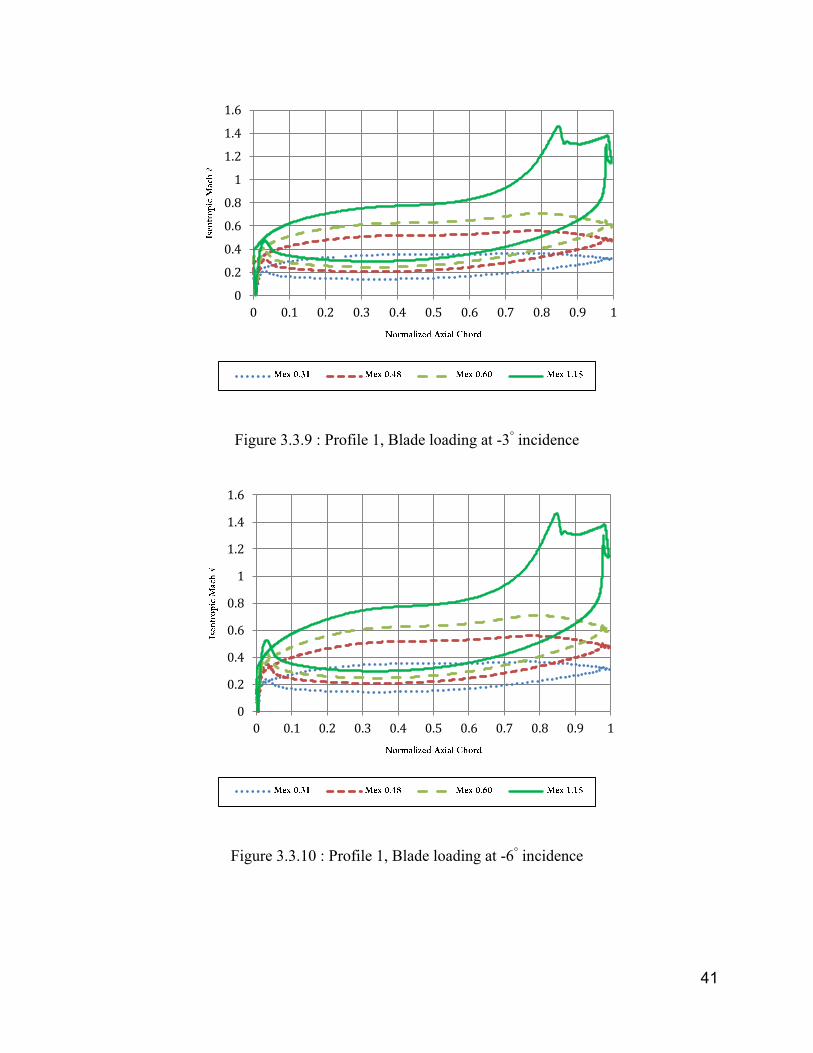
Figure 3.3.9 : Profile 1, Blade loading at -3° incidence ................................................................ 41
Figure 3.3.10 : Profile 1, Blade loading at -6° incidence .............................................................. 41
Figure 3.3.11 : Profile 1, Loss coefficient vs. Mex, 0° incidence ................................................. 42
Figure 3.3.12 : Profile 1, Loss Coefficient vs. Pitch, 0° incidence ............................................... 42
Figure 3.3.13 : Profile 1, Wake Profile, 0° incidence .................................................................... 43
Figure 3.3.14 : Profile 1, Avg Loss coefficient vs. Incidence Angle, Mex 0.48 ........................... 45
Figure 3.3.15 : Profile 1, Wake Profile, Mex 0.48 ........................................................................ 46
Figure 3.3.16 : Profile 1, Avg Loss coefficient vs. Incidence Angle ............................................ 46
Figure 3.3.17 : Profile 1, Wake Profile, Mex 0.31 ........................................................................ 47
Figure 3.3.18 : Profile 1, Wake Profile, Mex 0.60 ........................................................................ 48
Figure 3.3.19 : Profile 1, Wake Profile, Mex 1.15 ........................................................................ 48
Figure 3.4.1 : Profile 2, Blade loading at 0° incidence, design exit Mach 0.48 ............................ 49
Figure 3.4.2 : Profile 2, Pt variation across passage ..................................................................... 50
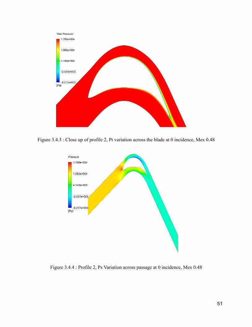
Figure 3.4.3 : Close up of profile 2, Pt variation across the blade at 0 incidence, Mex 0.48 ....... 51
Figure 3.4.4 : Profile 2, Ps Variation across passage at 0 incidence, Mex 0.48 ............................ 51
Figure 3.4.5 : Profile 2, Ps Variation across passage at 0° incidence, Mex 1.02 ........................... 52
Figure 3.4.6 : Profile 2, Blade loading at 0° incidence ................................................................. 53
Figure 3.4.7 : Profile 2, Blade loading at +3° incidence ............................................................... 54
Figure 3.4.8 : Profile 2, Blade loading at +6° incidence ............................................................... 54
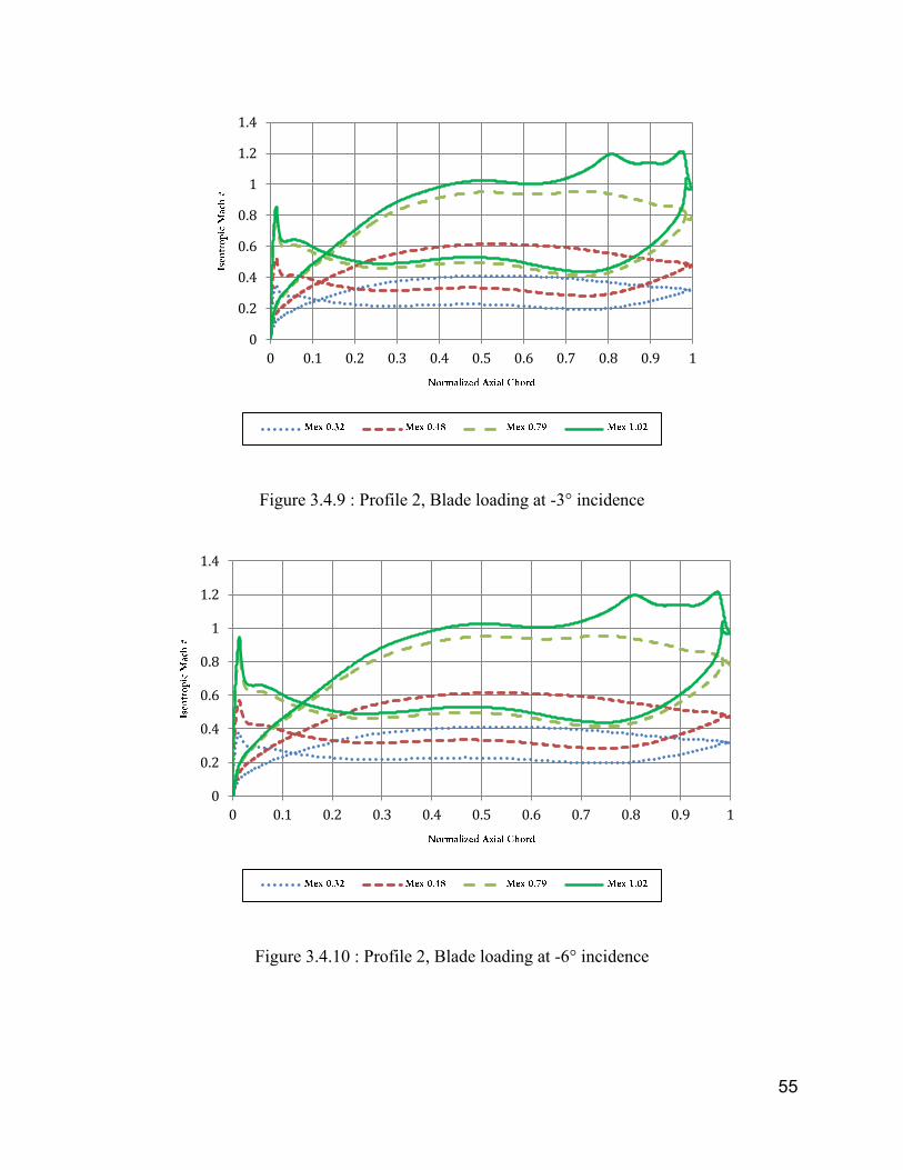
Figure 3.4.9 : Profile 2, Blade loading at -3° incidence ................................................................ 55

x
Figure 3.4.10 : Profile 2, Blade loading at -6° incidence .............................................................. 55
Figure 3.4.11 : Profile 2, Loss coefficient vs. Mex, 0° incidence ................................................. 56
Figure 3.4.12 : Loss Coefficient vs. Pitch, 0° incidence ............................................................... 56
Figure 3.4.13 : Profile 2, Wake Profile, 0° incidence .................................................................... 57
Figure 3.4.14 : Profile 2, Avg Loss coefficient vs. Incidence Angle, Mex 0.48 ........................... 58
Figure 3.4.15 : Profile 2, Wake Profile, Mex 0.48 ........................................................................ 58
Figure 3.4.16 : Profile 2, Avg Loss coefficient vs. Incidence Angle ............................................ 59
Figure 3.4.17 : Profile 2, Wake Profile, Mex 0.32 ........................................................................ 60
Figure 3.4.18 : Profile 2, Wake Profile, Mex 0.79 ........................................................................ 60
Figure 3.4.19 : Profile 2, Wake Profile, Mex 1.02 ........................................................................ 61
Figure 3.5.1 : Profile 2, Loss comparison between Profile 1 and 2, Mex 0.48............................. 62
Figure 3.5.2 : Profile 1, Blade Loading, Mex 0.48 ....................................................................... 63
Figure 3.5.3 : Profile 2, Blade Loading, Mex 0.48 ....................................................................... 64
Figure 3.5.4 : Profile 1, Deviation in Turning Angle vs. Incidence, Mex 0.48............................. 65
Figure 3.5.5 : Profile 2, Deviation in Turning Angle vs. Incidence, Mex 0.48............................. 66
Figure 3.6.1 : Loss Coefficient vs. exit Mach number (Song et al) [13] ...................................... 67
Figure 3.6.2 : Loss Coefficient vs. Incidence (Song et al) ............................................................ 68
Figure 3.6.3 : Loss coefficient vs. Mex, 0 incidence (Jouni et al) ................................................ 69
Figure 5.1.1 : Profile 1 Mesh ........................................................................................................ 73
Figure 5.1.2 : O-grid mesh structure around the leading edge for Profile 1 ................................. 74
Figure 5.1.3 : O-grid mesh structure around the trailing edge for Profile 1 ................................. 74
Figure 5.1.4: Mesh Independent grid for profile 1........................................................................ 75
Figure 5.2.1 Profile 4 Mesh .......................................................................................................... 76

xi
Figure 5.2.2 Profile 4, Blade loading, Mex 0.48, 0° incidence ..................................................... 77
Figure 5.2.3 : Profile 4, Loss coefficient vs. Mex, 0° incidence ................................................... 77
Figure 5.2.4 : Profile 2, Avg Loss coefficient vs. Incidence Angle, Mex 0.48 ............................. 78

xii
List of Tables
Table 2.2.1 : Blade Characteristics ............................................................................................... 14
Table 2.4.1 : Properties of the Meshes .......................................................................................... 17
Table 2.4.2 : Skewness vs. Cell quality ........................................................................................ 20
Table 2.5.1 : CFD Domain Properties .......................................................................................... 27
Table 2.5.2 : List of boundary conditions ..................................................................................... 27
Table 3.1.1 : Test Matrix for Profile 1 ........................................................................................... 30
Table 3.1.2 : Test Matrix for Profile 2 ........................................................................................... 30
Table 3.2.1 : Mesh Independence Results at 0 incidence, design exit Mach # ............................. 33
Table 5.2.1 : Test Matrix for Profile 4 ........................................................................................... 76

xiii
Nomenclature
βin Inlet Metal Angle
βout Outlet Metal Angle
Cax Axial Chord
LE Leading Edge
Mex Area Average Exit Mach Number
Min Area Average Inlet Mach Number
PS Pressure Side
Ps Static Pressure
Pt Total Pressure
SS Suction Side
TE Trailing Edge
To Total Temperature
u Velocity Component in x-direction
v Velocity Component in y-direction
w Velocity Component in z-direction
Y Loss Coefficient

xiv
γ Specific Heat Ratio
ν Kinematic Viscosity
ρ Density

1
1 Background & Introduction
There has been a perennial quest to increase turbine efficiencies in order to decrease fuel
consumption with the ultimate goal of reducing operating costs. The performance of the blades
and the losses at an operating condition are themselves a function of various factors, some of which
have been described below. Furthermore, a significant amount of time is spent operating at off
design conditions during which deviations from ideal conditions results in less than desired
efficiencies. Therefore, blades are designed with the intention to produce low losses at design
conditions and acceptable losses at off design conditions. As mentioned earlier losses are
themselves a function of various parameters, some of them being blade geometry, angle of
incidence, inlet/exit Mach numbers, pitch to chord ratio, end wall geometries and turbulence. Over
the past few decades, a large amount of effort has been made to better understand the origins of
losses as well as predict their magnitudes in order to aid in the design of better turbines.
Traditionally, losses as well as trends were documented by performing experiments in wind tunnels
using linear cascades; however, due to large gains in processor speeds and well as improvements
in numerical modelling over the last two decades, Computational Fluid Dynamics (CFD) is
increasingly being used to characterize losses and optimize designs. Commercial CFD solvers
utilizing popular turbulence models have been shown to characterize both the magnitude as well
as trends of losses fairly well.

2
1.1 Mechanism of Losses
The general consensus within both the academic community and industry is that losses within
turbines and compressors can be divided into three distinct types i.e. Profile losses, Secondary
flow losses and Tip losses. The latter two are due to the presence of an end wall and gaps between
casing and blades and in most cases are effects due to the three dimensionality of the flow field.
Profile losses on the other hand are accounted by the flow over the blades and can in many cases
be characterized by a two dimensional flow field. Many investigators have further broken down
profile losses into three inter related parts namely boundary layer losses, mixing losses and shock
losses. As the name suggests, boundary layer losses primarily arise within the boundary layer that
forms over the blade surface. Mixing losses result from the merging of the two different flow fields
from the suction and pressure side into a uniform flow field.
The fundamental mechanism for the generation of losses arises from entropy creation[1]. In the
absence of heat transfer within a passage, entropy is generated by viscous dissipation within
boundary layers and mixing layers. The rate of specific entropy generation within a boundary layer
is given by
�̇�𝑣 =
1
𝑇𝜏
𝑑𝑉
𝑑𝑦
Equation 1.1.1
Where, 𝜏 𝑑𝑉
𝑑𝑦 is the shear work. Based on the above formulation, it is evident that the region within
the boundary layer where the velocity changes rapidly would contribute the most towards entropy
generation. For turbulent boundary layers, this region falls within the laminar sub layer and

3
logarithmic region. At a fundamental level, this entropy increase represents the conversion of
kinetic or pressure energy of a fluid element into internal energy, which at a macroscopic level
translates to an increase in temperature.
In the case of mixing, the principle is the same as it is with boundary layers, the existence of shear
layer between fluid elements. This is primarily due to the difference in velocity of different fluid
elements leaving the suction and pressure side of the blade.
Lastly, in a fluid, shock waves exist due to fact that the medium is moving at speed faster than
information can propagate within the surrounding medium. It is an inefficient compression process
and is accompanied by a sharp increase in entropy and decrease in total pressure due to
redistribution of energy from velocity and pressure into internal energy of fluid element.
1.2 Loss Definition
There are different definitions of loss coefficients for cascade measurements. A compilation of loss
definitions as they apply to compressor and turbine cascades, as well as their relationship with
each other has been explained in [2].
For this thesis, the loss coefficient will be defined in the following manner.
𝑌 =
𝑃𝑡1 − 𝑃𝑡2
𝑃𝑡2 − 𝑃𝑠2
Equation 1.2.1

4
Once the loss plot is generated from taking local values of above variables, the loss coefficient is
determined by numerically integrating the curve and averaging it with the pitch. Values of Pt2 and
Ps2 are taken from a plane 0.3 axial chords downstream of the trailing edge.
The isentropic Mach number used in describing the blade loading can be computed using the
relation below where, Pt1 represents the inlet total pressure and Ps represents the local static
pressure over the blade surface. The specific heat ratio of air (γ) is taken to be 1.4 and assumed be
constant.
Equation 1.2.2
At downstream plane, the total pressure ratio has been defined as follows.
𝑇𝑜𝑡𝑎𝑙 𝑃𝑟𝑒𝑠𝑠𝑢𝑟𝑒 𝑅𝑎𝑡𝑖𝑜 =
𝑃𝑡2
𝑃𝑡1
Equation 1.2.3
𝑀 = √((𝑃𝑡1
𝑃𝑠)
(𝛾−1)𝛾
− 1 ) .2
𝛾 − 1

5
1.3 Literature Survey
Hoheisel et al[3] investigated the effects of free stream turbulence and blade pressure gradient on
boundary layer and loss behavior of turbine cascades. In this experiment, a turbulence intensity of
up to 8% were generated and the behavior on transition of the boundary layer on a forward loaded
blade and two aft loaded blades were studied. The authors noted that the aft loaded blade with
carefully limited rearward deceleration performed best in terms of total pressure loss. At turbulent
intensity levels greater than 2%, the aft loaded velocity distribution performed better than their
front loaded counterpart. This was true even at the design Reynolds number where the turbulence
intensity levels had a stronger impact on front loaded cascade. The authors also concluded that
even at off design incidences and high subcritical Mach numbers, the aft loaded blades were more
efficient.
On a two dimensional linear turbine cascade, Mee et al [4] investigated the contributions of
boundary layer losses, shock wave losses and mixing losses to the overall profile loss as a function
of exit mach number. The authors noted that the mixing loss is similar in magnitude to the
boundary layer losses but remained less than the boundary layer losses up to an exit mach number
of 1.02. At even higher exit mach numbers, the mixing losses dominated the contribution towards
the overall losses. In regards to shock losses, the authors noted for this set of geometry, the shock
losses were absent till an exit mach number of 0.95. The shock losses at first seemed to decrease
as the exit mach number increased. The authors noted that this observation is spurious and that the
reason for this is the way the losses have been computed. A significant portions of the shock losses
6
at higher exit mach numbers occurred at plain further downstream of the measurement plane. In
this experiment, the authors also noted that most of the mixing loss is generated immediately
downstream of the trailing edge of the blade where the gradients in properties across the wake are
largest. On an additional note, the width of wake increased as a square root of distance downstream
of the blade.
The state of the boundary layer has a very strong effect on the total pressure losses
downstream of the blade. Turbulent boundary layers, which enhance mixing, tend to increase
losses so understanding the transition characteristics of boundary layers is of vital importance. In
this regard, Rivir [5] investigated the effects of inlet turbulent intensity, solidity and turbulence
length scales on the location of the start of transition as well as their impacts on the length of
transition zone. The experiments were performed on a low pressure turbine cascade at low
Reynold’s numbers. The authors reported that for a fixed Reynold’s number, increasing the
turbulence intensity for this cascade caused the transition point to move forward while
simultaneously increasing the length of the transition zone. Furthermore, the authors also noted
that for a constant turbulence intensity of 10%, the transition location was unaffected by the length
scale however, the experiments with larger length scales had longer transition lengths.
Brear et al[6] investigated the effects pressure side surface separations on thin 2-D low
pressure blades with measurement taken at midspan. The authors concluded that separation from
the pressure side can have a significant impact on loss measurements and that the size of the
pressure surface separation increases considerably with reduced incidence. The authors noted that
the adverse pressure gradient is determined to a great extent by the flow incidence angle which
controlled the spikes in velocity at the leading edge. They used smoke wire flow visualization at a

7
+10 and -10 degree incidences and noticed that midspan vortices formed at the pressure size which
rapidly increases in size as they move downward.
M. Li et al [7] studied the loss behavior of two high pressure steam turbine blades at
extreme off design incidences. Three incidences were tested over a range of Mach numbers i.e -
25, 5 and 35 degrees. The authors noted that the trend for all incidences were the same with Mach
number. The losses were insensitive to Mach number in the subsonic exit Mach number range. In
the transonic and supersonic regimes, the presence of shocks caused a steep increase in losses. The
authors noted that losses were lowest at design incidence angle of 5 degrees. The authors also
noted that the losses were more sensitive to increasing Mach number than they were to extreme
incidences. Maximum losses, due to extreme change in incidence angle (35 degrees), was around
twice as high compared to design incidence angle. The losses for all incidence angles peaked with
Mach number and then started to decrease. The authors noted that the reason for this behavior was
the following, as the exit Mach number increased, the flow at the trailing edge separated due to
the interaction between boundary layer and a shock. The interaction of the shock with the wake of
another blade increased mixing losses. As the Mach number increased additional shocks appeared
on the pressure side of the blade and interacted with the boundary layer of the blade which resulted
in additional losses. However, further increase in Mach number lead to the formation of oblique
shocks which lowered losses. Finally, the authors noted that the blade with a higher solidity had
higher losses in the transonic regime due to stronger shock wave interaction with trailing edge
wakes.
On the numerical side of things, In a study, Sanz et al [8], using 2-D Navier Stokes solver computed
the flow field over a linear turbine cascade using two different turbulence models i.e. the one
equation Spalart-Allmaras(SA) and the two equation low Reynold’s number k-ε model. The
8
objective of this study was to compute the downstream wake profile, at three different stations,
and compare the results to the experimental data. The authors found out that near the trailing edge,
the computed velocity defect using both turbulence models showed poor agreement with the
measured values. The authors attributed this to the fact that in the experiments, a periodic wake
sheading was observed at the trailing edge and the steady numerical simulations couldn’t capture
this effect. However, the disparity between simulations and experiment lessened as the distance
from the trailing edge increased. Another key observation was the fact that despite showing
asymmetry in the wake profile by both the experiments and simulations, the asymmetries were on
different sides. Numerical simulations predicted a wider wake on the suction side, which was also
reported by previous authors, whereas experiments predicted a wider wake on the pressure side.
In a another numerical study on 2-D linear cascades conducted by Hesham El-Batsch [9], the
ability of numerics, using two turbulence models (Spallart-Allmaras and k-ε model), to accurately
replicate experimental results was studied. The blade loading at design and off design conditions
was predicted fairly well using either turbulence model. The slight disparity in blade loading at an
off design incidence of 10 towards the trailing edge has been attributed to the formation of a shock
in the CFD. Since fully turbulent models were used, the total pressure coefficient curves at a
downstream wake location were deeper and thicker than experimental predictions. However, the
wake profile predicted using SA was in better agreement with experimental data. In regards to the
total pressure loss coefficient, the simulations predicted higher losses owing to the fact that they
use a fully turbulent assumption. However, for the most part the trends were maintained with the
exception of the +10 off design case.
More recently, Martinstetter et al [10] used experimental and computational data to study the
effects of inflow turbulence intensity on the loss behavior of highly loaded Low pressure turbine

9
cascade. They noted the following that at low Reynolds number, higher inlet turbulence had a net
positive effect on the laminar separation bubble and reduced losses. At higher Reynolds number,
the higher inflow turbulence levels had no net impact on the losses.
Abraham and Panchal et al [11] used numerical and experimental methods to study the impact of
a divergent end wall on turbine losses. In this study, SST turbulence model was used in the
numerical study and as able to track experimental results, both the magnitude and trends,
exceptionally well.

10
2 Geometry Preparation and Modeling
2.1 Overview
This chapter will go over the steps used in order to simulate the flow field around the domain of
interest as well as characterize the blade properties. The following procedure was repeated for each
of the blade profiles:
Steps Software Used
Export Mesh into a CFD solver, impose appropriate boundary conditions and
run simulations.
Extraction of fluid volume from CAD model of turbine cascade.
Import an IGES file in to grid generator and construct a mesh.
Export CFD results into post processor to visualize and extract data.
SolidWorks (ver 2012)
Pointwise (ver 17)
Ansys CFX (ver 13)
Ansys Post, Matlab, Microsoft Excel

11
2.2 Blade Geometries
A set of three steam turbine airfoils were provided in iges format. These files were processed using
popular CAD software SolidWorks (Version 2012). The pitches for all three blades was kept at 2.5
inches, in order to kept the solidity the same as it was with the original configuration, the blades
were scaled accordingly. The three blade profiles are shown in the figures below.
Figure 2.2.1: Baseline Profile
12
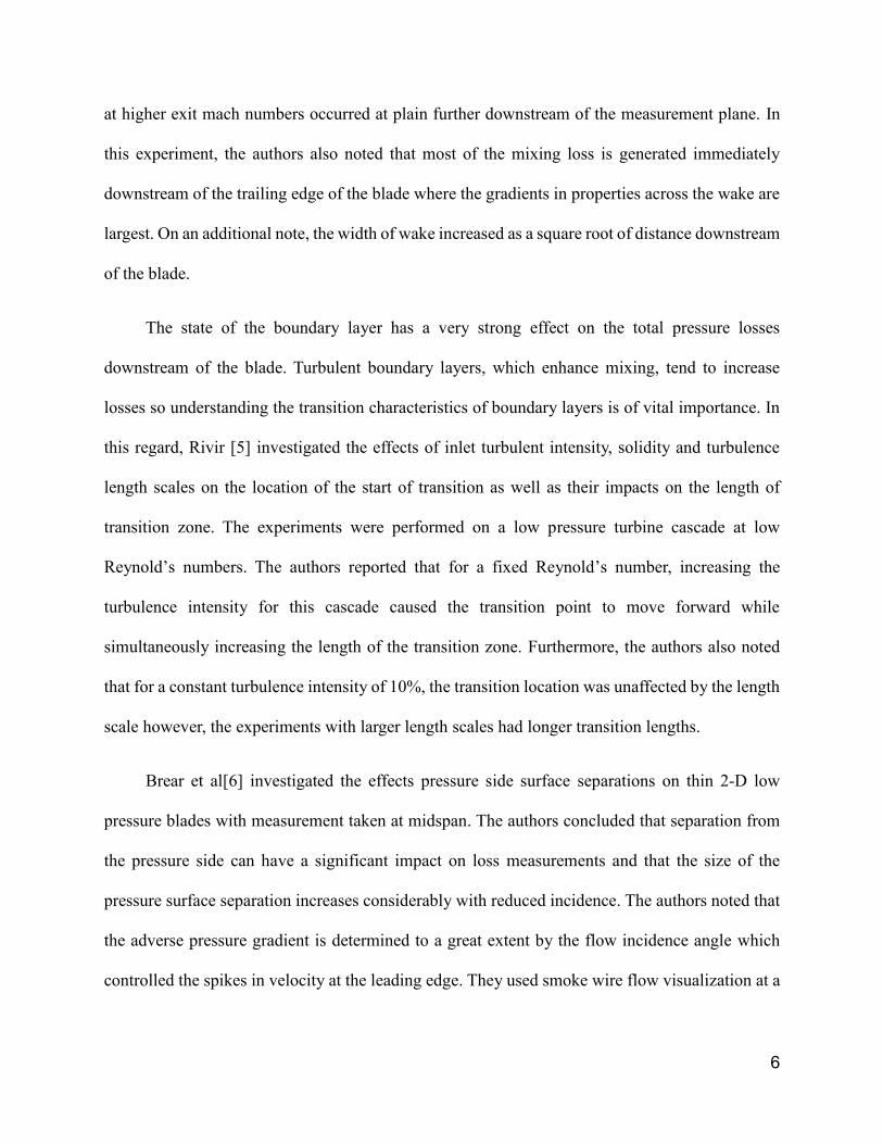
Figure 2.2.2 : Blade 2 (Pitch line profile)
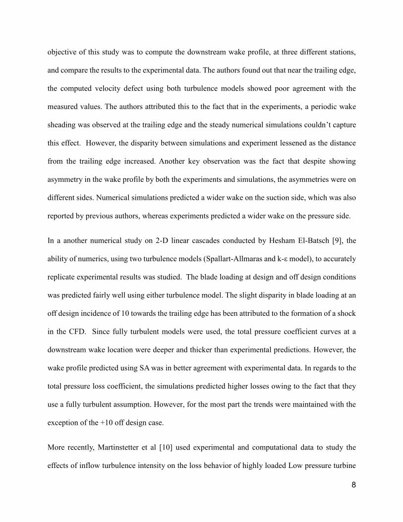
Figure 2.2.3 : Blade 3 (Tip profile)

13
Figure 2.2.4 : Blade Nomenclature (a)
Figure 2.2.5 : Blade Nomenclature (b)
Pitch

14
Table 2.2.1 : Blade Characteristics
Axial Chord
(in)
Inlet Metal
Angle
(Deg)
Exit Metal
Angle
(Deg)
Blade 1 : Baseline
Profile
3.72 30.2 20.53
Blade 2 : Mean line
Profile
3.68 43.29 24.53
Blade 3 : Tip Profile 3.62 50.03 23.98
Incidence angle has been defined as the angle the flow makes with respect to the tangent at the
chamberline from the leading edge, when it enters the domain, at the inlet. Based on the figures
provided, blades 2 and 3 do exhibit a similar geometric profile as they represent the mid radius
and tip sections of a single high pressure steam turbine rotor blade respectively. The pitch of the
blades (distance between successive blades) is 2.5 inches for all three turbine cascades.
15
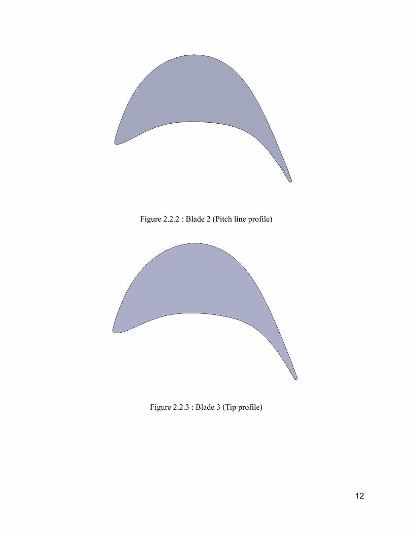
2.3 Fluid Domain and Geometry Set Up
The passage geometry was extracted from a CAD model of a linear turbine cascade in SolidWorks.
The upper and lower periodic lines were generated by extending the blade chamberline 1.25 inches
above and below the blade. In order to allow the flow enough time to develop, the inlet was placed
around two axial chords ahead of the leading edge along the blade metal angle, while the outlet
was placed at a distance of about three axial chords behind the trailing edge along the blade exit
angle. The figure below provides a description of the passage geometry used in the CFD
computations. For the sake of brevity, only the mid radius blade (profile 2) passage has been
shown. The exact same procedure was used for the other two blades.
Figure 2.3.1 : Geometry of Profile 2 Passage

16
2.4 Mesh Generation and Metrics
The extracted fluid domain passage was meshed in Pointwise (Version 17), popular meshing
software. In order to accurately capture all essential details of the flow while simultaneously
keeping the total number of cells relatively low, a multiblock structured domain approach was
used. A single block approach would be the simplest approach however, it is highly inefficient.
For example, an O-grid mesh technique would be sufficient to capture all details of the flow
through the passage however, in order to resolve the flow downstream of the blade, the O-grid
lines would be automatically be extended upwards thereby resulting in an unnecessary increase in
grid size. A single H-type grid could work; however, it would have a very poor mesh quality around
the highly curved leading and trailing edges. Therefore a mixed blocking approach was the most
practical method.
First, a surface extrusion process was used to generate a fine grid O grid that encapsulated the
airfoil surface. In order to keep the dimensionless Y plus value around or below 1, over a range of
flow velocities, the initial wall spacing was set to 0.5 µm. Using a growth ratio of 1.1, the mesh
was extruded to around 60 layers. Following this, the passage was systematically divided into
multiple H type grid blocks in order to create high quality structured grids. A close up of the
division of geometry into multiple domains has been shown below for the Profile 2 passage
(demarcated in red).

17
Figure 2.4.1 : Profile 2 Mesh
As can be seen from Figure 2.3.1, the entire passage has been divided into multiple blocks; a thin
O-type grid surrounds the blade while the rest of the grid has been split up into multiple H-blocks.
The sole reason for having multiple H-type blocks is to allow greater control over the quality of
the mesh. These blocks were merged prior to exporting them to a CFD solver. Another fact to note
is that the upper and lower periodic surfaces are non-conformal (i.e. they have different number of
cells). This is not an issue as ANSYS CFX can handle non conformal periodic grids.
Table 2.4.1 : Properties of the Meshes
Profile No of Cells Type
Baseline Blade (1) 288,047 Multi block Structured
Mid Radius (2) 261,667 Multi block Structured
Tip Radius (3) 292,816 Multi block Structured
18
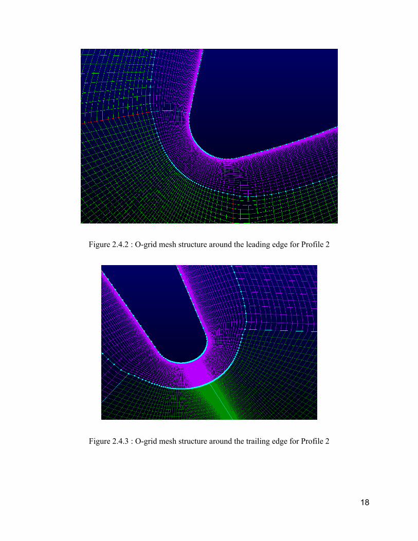
Figure 2.4.2 : O-grid mesh structure around the leading edge for Profile 2
Figure 2.4.3 : O-grid mesh structure around the trailing edge for Profile 2
19
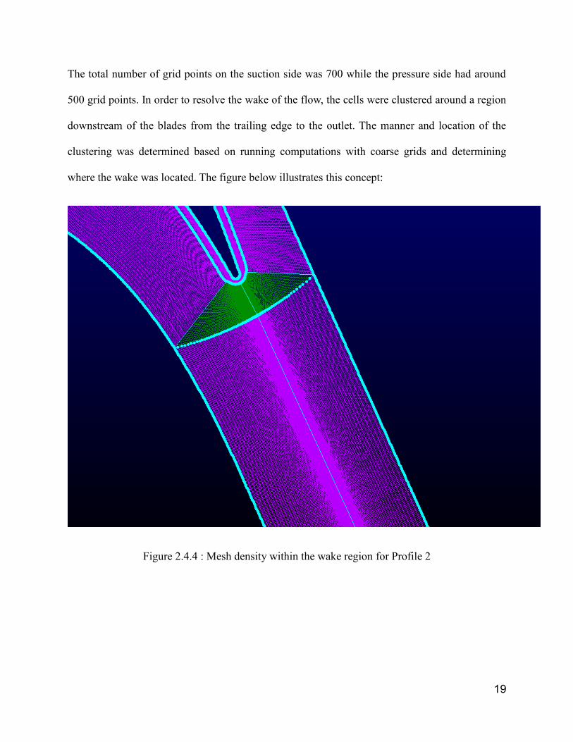
The total number of grid points on the suction side was 700 while the pressure side had around
500 grid points. In order to resolve the wake of the flow, the cells were clustered around a region
downstream of the blades from the trailing edge to the outlet. The manner and location of the
clustering was determined based on running computations with coarse grids and determining
where the wake was located. The figure below illustrates this concept:
Figure 2.4.4 : Mesh density within the wake region for Profile 2

20
2.4.1 Mesh Metrics
In order to get good computational results it is imperative to have a high quality mesh. There are
many different parameters that can be used to quantify the quality of a mesh, some of which are
listed below.
Quality Parameters:
1. Equiangular Skewness1: Essentially determines how close a face/cell is to an ideal
equiangular quadrilateral or triangle. The formula for this computation is
𝐸𝑞𝑢𝑖𝑎𝑛𝑔𝑢𝑙𝑎𝑟 𝑆𝑘𝑒𝑤 = max (𝜃𝑚𝑎𝑥 − 𝜃𝑒
180 − 𝜃𝑒,𝜃𝑒 − 𝜃𝑚𝑖𝑛
𝜃𝑒)
where,
θmax = Largest angle in a face/cell
θmin = Smallest angle in a face/cell
θe = equiangle for a face/cell. 60̊ for triangles and 90̊ for quadrilaterals.
Table 2.4.2 : Skewness vs. Cell quality
Value of Skewness Cell Quality
0.90 - <1 bad
0.75 - 0.90 poor
0.50 - 0.75 fair
0.25 - 0.50 good
>0 - 0.25 excellent
0 equilateral
Aspect Ratio: It is defined as the ratio of the longest side of a face/cell to its shortest. In essence,
it is a measure of how much a face/cell is stretched. An ideal aspect ratio is 1. However, within
1 1 http://www.sharcnet.ca/Software/Fluent13, Ansys fluent help file.

21
the boundary layer, it is very common to have cells with large aspect ratios (>100) as the flow
gradients change rapidly in a direction normal to a streamline than along it.
Figure 2.4.5: Profile 2, LE Equiangular Skewness

22
Figure 2.4.6 : Profile 2, TE Equiangular Skewness
Figure 2.4.7 : Profile 2, Region of high Skew

23
2.4.2 Discussion of Mesh Metrics
Table 2.4.2 and the above figures illustrate that the O-grid wrapped around the blade has a very
low equiangular skew. H-grids that constitute the rest of the mesh have a low skew with the
exception of the region near the outlet (see Figure 2.4.7). Due to the nature of the geometry, and
Figure 2.4.8 : Profile 2, Region of high aspect ratio

24
the strict requirement of being a pure structured mesh, the level of skew towards the end had to
be fairly high. However, the moderately high level of skew has little influence on the accuracy of
the solution as the flow in this region is not changing in properties, is unidirectional and the losses
have mixed out. This statement is later shown to be true in the grid independence study.
High aspect ratio cells (Aspect ratio > 100) are all limited to the cells within O-grid next to the
wall. It is a very common practice to have inflation layers with high aspect ratios as the gradients
within the boundary layer change rapidly normal to the surface as opposed to along the surface.
Outside the boundary layer, the cells have a very low aspect ratio, which is desirable. The cells
with the maximum aspect ratio, outside the boundary layer, are those within the wake region
(aspect ratio ~40).

25
2.5 CFD Solver & Theory
The solver that was used to compute the flow field was Ansys CFX (Ver 13). Ansys CFX is a
vertex-centered finite volume based computational solver in which, the governing equations of
fluid dynamics (Navier-Stokes) are discretized using their conservation form. These discretized
equations are then numerically solved using various mathematical approaches at each grid point
on a mesh.
The single phase unsteady Navier-Stokes equations in their differential equation form are provided
Continuity of Mass
𝑑𝜌
𝑑𝑡+
𝑑𝜌𝑢
𝑑𝑥+
𝑑𝜌𝑣
𝑑𝑦+
𝑑𝜌𝑤
𝑑𝑧= 0
Continuity of Momentum
𝑑𝜌𝑢
𝑑𝑡+
𝑑𝜌𝑢2
𝑑𝑥+
𝑑𝜌𝑢𝑣
𝑑𝑦+
𝑑𝜌𝑢𝑤
𝑑𝑧= −
𝑑𝑝
𝑑𝑥+ 𝜗 (
𝑑2𝑢
𝑑𝑥2+
𝑑2𝑢
𝑑𝑦2+
𝑑2𝑢
𝑑𝑧2)
𝑑𝜌𝑣
𝑑𝑡+
𝑑𝜌𝑢𝑣
𝑑𝑥+
𝑑𝜌𝑣2
𝑑𝑦+
𝑑𝜌𝑣𝑤
𝑑𝑧= −
𝑑𝑝
𝑑𝑦+ 𝜗 (
𝑑2𝑣
𝑑𝑥2+
𝑑2𝑣
𝑑𝑦2+
𝑑2𝑣
𝑑𝑧2)
𝑑𝜌𝑤
𝑑𝑡+
𝑑𝜌𝑢𝑤
𝑑𝑥+
𝑑𝜌𝑣𝑤
𝑑𝑦+
𝑑𝜌𝑤2
𝑑𝑧= −
𝑑𝑝
𝑑𝑧+ 𝜗 (
𝑑2𝑤
𝑑𝑥2+
𝑑2𝑤
𝑑𝑦2+
𝑑2
𝑑𝑧2)
Conservation of Energy

26
𝑑𝜌𝐸
𝑑𝑡+
𝑑𝜌𝑢𝐸
𝑑𝑥+
𝑑𝜌𝑣𝐸
𝑑𝑦+
𝑑𝜌𝑤𝐸
𝑑𝑧= −
𝑑𝑝𝑢
𝑑𝑥−
𝑑𝑝𝑣
𝑑𝑥−
𝑑𝑝𝑤
𝑑𝑥+ 𝑆
In the above equations, E and S are the internal energy and source terms respectfully.
2.5.1 Boundary Conditions

27
Table 2.5.1 : CFD Domain Properties
Domain Properties Characteristics
Material Air Ideal Gas
Reference Pressure 1 atm
Heat Transfer/ Fluid Model Total Energy
Turbulence Model Shear Stress Transport
Table 2.5.2 : List of boundary conditions
Boundary condition Type Characteristics
Inlet Total Pressure Inlet Total Pressure : Variable
Inlet Temperature : 300 K
Inlet Tu : 4%
Inlet length scale : 0.009 m
Outlet Static Pressure Relative Pressure : 0 Pa
Periodic Translational Periodicity Automatic
Wall Adiabatic, no slip condition -
For all profiles, at all flow conditions, the downstream static pressure was kept at 0 gauge
pressure. The reference pressure was fixed at 1 atm. In addition, since the flow regime of interest
was of high Mach number, the full set of Navier Stoke equations had to be solved. This was
achieved by turning on the total energy option in CFX. In addition, a static temperature of 300 K
was fixed at the inlet. The exit Mach numbers were computed by entering appropriate values of
inlet total pressure. In addition to the above boundary conditions, an extra boundary condition
had to be applied to simulate a 2-D flow field.
28
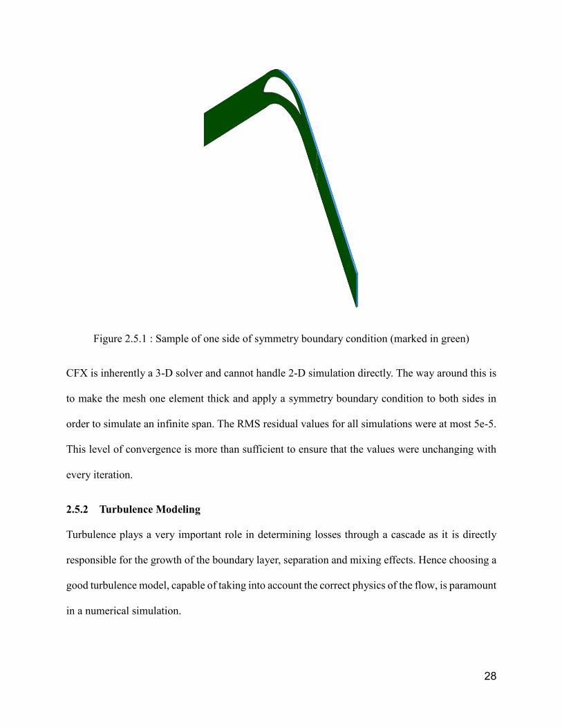
Figure 2.5.1 : Sample of one side of symmetry boundary condition (marked in green)
CFX is inherently a 3-D solver and cannot handle 2-D simulation directly. The way around this is
to make the mesh one element thick and apply a symmetry boundary condition to both sides in
order to simulate an infinite span. The RMS residual values for all simulations were at most 5e-5.
This level of convergence is more than sufficient to ensure that the values were unchanging with
every iteration.
2.5.2 Turbulence Modeling
Turbulence plays a very important role in determining losses through a cascade as it is directly
responsible for the growth of the boundary layer, separation and mixing effects. Hence choosing a
good turbulence model, capable of taking into account the correct physics of the flow, is paramount
in a numerical simulation.

29
In order to accomplish these tasks, Menter’s Shear Stress Transport (SST) was chosen to model
the turbulent characteristics of the flow. The SST turbulence model is a very popular two equation
turbulence model that was originally developed to model external aerodynamic flows where strong
adverse pressure gradients and separation were present [12]. The SST model at a fundamental
level is the fusion of the k-ε and k-ω turbulence models. Despite the k-ω model being more accurate
in modeling flows near the wall, it suffers from a few drawbacks one of which is its strong
sensitivity to freestream turbulence. Additionally, k-ε gives poor performance for flows with
strong adverse pressure separations. The SST model uses a blending function to determine when
to use the k-ω or k-ε model, which is based on the distance of a mesh node from the wall. The
formulation originally proposed by Menter to model the turbulent kinetic energy as well as
dissipation has been provided below:
Figure 2.5.2 : SST model formulation [12]
In the above equation, F1 is a parameter that determines the switch between the k-ω and k- ε
respectively. Its value is zero away from the boundary layer and one within the boundary layer. As
described in the previous sections, the grid was created such that the y+ values were close to or
below 1. This allows the SST model to resolve the flow within the laminar sub layer without the
use of any wall functions. The descriptions as well as details of all the terms are provided in the
reference.

30
3 Results and Discussion
3.1 Test Matrix
The goal of this research was to characterize the performance of three high pressure steam turbine
airfoils at various exit Mach numbers and incidences. However it was found out that profiles 2 and
3 (mid radius and tip profiles) showed near identical performance as well as blade loading. Hence
only results of profiles 1 and 2 will be discussed. Data for profile 3 has been included in the
appendix. A test matrix was created for the two profiles and the simulations were then conducted
at these selected conditions. The test matrix has been provided below:
Table 3.1.1 : Test Matrix for Profile 1
Incidences Exit Mach #
-6, -3, 0, +3, +6 0.31
-6, -3, 0, +3, +6 0.48 (design)
-6, -3, 0, +3, +6 0.60
0 0.79
-6, -3, 0, +3, +6 1.15
Table 3.1.2 : Test Matrix for Profile 2
Incidences Exit Mach #

31
-6, -3, 0, +3, +6 0.32
-6, -3, 0, +3, +6 0.48 (design)
-6, -3, 0, +3, +6 0.79
-6, -3, 0, +3, +6 1.02
For profile 1, the Reynold’s number based on axial chord ranged from 650,000 to 2,600,000. The
largest Yplus value recorded for all the simulations was 0.9. Similarly, for profile 2, the
Reynold’s number based on axial chord ranged from 640,000 to 2,250,000. The largest Yplus
value recorded was 0.85.

32
3.2 Mesh Independence Study
In order to ensure that the results were independent of the type of mesh and its density, an
alternative mesh was created for both profile 1 & 2. Since the boundary layer around the blade had
been sufficiently well resolved, only the region in the wake needed to be checked for grid
independence. On the mesh figures in the previous sections, in the region around the wake, the
cells were tightly clustered. As mentioned earlier, the location and clustering of the cells was based
on an iterative procedure for both the profiles. However, since loss coefficients were calculated
by numerically integrating the data in the wake region, errors could have been induced due to lack
of sufficient data points. Along similar lines, the clustering of the cells in the wake region might
have left far out regions with insufficient resolution to characterize gradients in flow properties,
despite them being small. Finally, as shown in Figure 2.4.7, regions of high skewed cells existed
near the outlet of the flow which potentially could induce numerical errors.
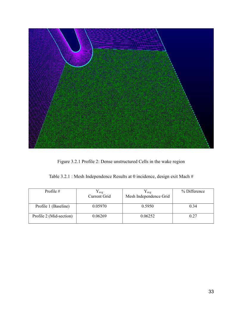
In order to alleviate these concerns, a separate mesh was constructed replacing the entire wake
region with a highly dense uniform unstructured mesh. The total number of cells within the wake
region for the mesh independence study was around 1.6 million. The simulation was only
conducted only at the design exit Mach number of 0.48 at 0 incidence. It has been shown in Table
3.2.1, that the simulations are grid independent.
33
Figure 3.2.1 Profile 2: Dense unstructured Cells in the wake region
Table 3.2.1 : Mesh Independence Results at 0 incidence, design exit Mach #
Profile # Yavg
Current Grid
Yavg
Mesh Independence Grid
% Difference
Profile 1 (Baseline) 0.05970 0.5950 0.34
Profile 2 (Mid-section) 0.06269 0.06252 0.27

34
3.3 Profile 1 (Baseline)
3.3.1 Blade Loading
Figure 3.3.1 : Profile 1 Blade loading at 0 incidence, design exit Mach 0.48
Since part of the losses is generated within the boundary layer of the blade, it is imperative to study
the blade loading as the pressure distribution over the blade, as it is responsible for the growth and
evolution of the boundary layer. Looking at the above plot, towards the leading edge of the blade,
starting from the stagnation point, there is rapid acceleration over the surface of the blade on both
the PS as well as SS of the blade. However, past a normalized axial chord value of 0.05, a zone of
deceleration exists over the PS of the blade which exists up to a normalized axial chord value of
around 0.4. From then onwards, a favorable pressure gradient exists on the entirety of the PS. On
0
0.2
0.4
0.6
0 0.1 0.2 0.3 0.4 0.5 0.6 0.7 0.8 0.9 1
SS
PS

35
the SS, a favorable pressure gradient exists for a major portion of the blade surface until a
normalized axial chord value of 0.75. Past this point, an adverse pressure gradient develops over
the SS of the blade. On an overall scale, there is no indication of significant flow acceleration on
either SS or PS. The change in Mach number over the surface of the blade is fairly gradual.
Figure 3.3.2 : Profile 1, Pt variation across the blade at 0° incidence, Mex 0.48
36
Figure 3.3.3 : Close up of profile 1, Pt variation across the blade at 0° incidence, Mex 0.48
Figure 3.3.4 : Profile 1, Ps Variation across passage at 0° incidence, Mex 0.48
Looking at Figure 3.3.3, the growth of the boundary layer over the SS and PS is evident. The red
portion of the graph represents the inviscid core while the rest of the color band represents the total

37
pressure within the boundary layer. The legend to the right represents the total pressure in gauge
(reference pressure is 1 atm).
However, it is evident that most of the loss is generated over the SS while the PS boundary layer
is thin and contributes very little to the overall losses generated. The SS side generated losses are
greater for two reasons, the first one being the fact that the SS is longer in length than the PS,
which allows greater room for the boundary layer to grow. More importantly, the presence of an
adverse pressure gradient towards the trailing edge of the suction side causes a rapid thickening of
the boundary layer which results in higher losses for the SS.
Figure 3.3.6 shows the variation of the blade loading at 0° incidence as a function of exit Mach
number. The above discussion holds true for increasing Mach number with the exception of
supersonic exit Mach number case (Mex 1.15). For a Mex of 1.15, the flow goes past supersonic
at the throat, rises to a maximum and then passes through an oblique shock and then decelerates.
38
Figure 3.3.5 : Profile 1, Ps Variation across passage at 0° incidence, Mex 1.15
39
Figure 3.3.6 : Profile 1, Blade loading at 0° incidence
0
0.2
0.4
0.6
0.8
1
1.2
1.4
1.6
0 0.1 0.2 0.3 0.4 0.5 0.6 0.7 0.8 0.9 1

40
Figure 3.3.7 : Profile 1, Blade loading at +3° incidence
Figure 3.3.8 : Profile 1, Blade loading at +6° incidence
0
0.2
0.4
0.6
0.8
1
1.2
1.4
1.6
0 0.1 0.2 0.3 0.4 0.5 0.6 0.7 0.8 0.9 1
0
0.2
0.4
0.6
0.8
1
1.2
1.4
1.6
0 0.1 0.2 0.3 0.4 0.5 0.6 0.7 0.8 0.9 1
41
Figure 3.3.9 : Profile 1, Blade loading at -3° incidence
Figure 3.3.10 : Profile 1, Blade loading at -6° incidence
0
0.2
0.4
0.6
0.8
1
1.2
1.4
1.6
0 0.1 0.2 0.3 0.4 0.5 0.6 0.7 0.8 0.9 1
0
0.2
0.4
0.6
0.8
1
1.2
1.4
1.6
0 0.1 0.2 0.3 0.4 0.5 0.6 0.7 0.8 0.9 1

42
3.3.2 Variation of Loss Coefficient with Exit Mach Number
Figure 3.3.11 : Profile 1, Loss coefficient vs. Mex, 0° incidence
Figure 3.3.12 : Profile 1, Loss Coefficient vs. Pitch, 0° incidence
0
0.02
0.04
0.06
0.08
0.1
0.25 0.35 0.45 0.55 0.65 0.75 0.85 0.95 1.05 1.15 1.25
0
0.1
0.2
0.3
0.4
0.5
0.6
-1.25 -0.625 0 0.625 1.25
)
Mex 0.31 Mex 0.48 Mex 0.60 Mex 0.79 Mex 1.15
P
S
SS

43
Figure 3.3.13 : Profile 1, Wake Profile, 0° incidence
The loss coefficient has been calculated using Equation 1.2.1, Figure 3.3.11 shows the variation of
the dimensionless loss coefficient vs. Mex. The loss coefficient decreases with Mex until the flow
over the blades reaches transonic Mach numbers. Due to the limited number of data points on the
graph, the increase in loss coefficient as the flow becomes transonic isn’t evident directly, but can
be inferred from the values of loss coefficient at supersonic exit Mach numbers. Figure 3.3.12
shows the variation of the loss coefficient with Mex at 0° incidence where the vertical line indicates
the geometric center of the passage. At subsonic Mach numbers, the peak of the loss coefficient is
almost the same. The overall width of the wake region also decreases with Mex. At supersonic
Mex, the presence of shock waves causes total pressure losses within the free stream and this,
coupled with an increase in static pressure behind the shocks, results in high losses. Commensurate
0.8
0.85
0.9
0.95
1
-1.25 -0.625 0 0.625 1.25
Mex 0.32 Mex 0.48 Mex 0.60 Mex 0.79 Mex 1.15
P
S
SS

44
with previous discussion, the wake shows that it is suction side heavy i.e. most of the total pressure
losses from the boundary layer as well as mixing occur from the suction side of the blade.
Figure 3.3.13, plots the ratio of the total pressure within the wake to that of the free stream vs.
Pitch for different Mex. The total pressure defect increases with Mex, which is a very expected
trend. The wake also shifts towards the geometric center of the passage, away from the suction
side, with increasing Mex. This is a result of boundary layer becoming thinner with increasing
Mex due to fact that the Reynold’s number is scaling with Mach number. It is apparent that the
peaks and of loss coefficients at the subsonic exit Mach number are the same. Yet the average loss
coefficient is decreasing with exit Mach number. This again is due to the fact that the boundary
layer is thicker at lower Mach numbers due to the Reynold’s number being lower.

45
3.3.3 Variation of Loss Coefficient with Incidence
Figure 3.3.14 : Profile 1, Avg Loss coefficient vs. Incidence Angle, Mex 0.48
Figure 3.3.14 indicates that for profile 1, at design Mex (0.48) the loss coefficient is sensitive to a
moderate change in incidence. The loss coefficients are highest at the positive incidences and based
on the trend, it appears to continue increasing. On the opposite spectrum, the loss coefficient
decreases with negative incidences and asymptotically reaches a value. Alternatively, this can be
identified directly by looking at the wake total pressure ratios in Figure 3.3.15 where, the wake
profiles at 0, -3 & -6 degrees incidence overlap .
0
0.02
0.04
0.06
0.08
0.1
-6 -3 0 3 6

46
Figure 3.3.15 : Profile 1, Wake Profile, Mex 0.48
Figure 3.3.16 : Profile 1, Avg Loss coefficient vs. Incidence Angle
0.85
0.9
0.95
1
-1.25 -0.625 0 0.625 1.25
0 Deg +3 Deg +6 Deg -3 Deg -6 Deg
0
0.02
0.04
0.06
0.08
0.1
-6 -3 0 3 6
Mex 0.48 Mex 0.31 Mex 0.60 Mex 1.15
P
S
SS

47
The loss coefficient trend is independent of Mex as Figure 3.3.16 shows. To further corroborate
this fact, the total pressure ratio plots at various Mex that have been shown below, support this
trend.
Figure 3.3.17 : Profile 1, Wake Profile, Mex 0.31
0.8
0.85
0.9
0.95
1
-1.25 -0.625 0 0.625 1.25
0 Deg +3 Deg +6 Deg -3 Deg -6 Deg
P
S
SS

48
Figure 3.3.18 : Profile 1, Wake Profile, Mex 0.60
Figure 3.3.19 : Profile 1, Wake Profile, Mex 1.15
0.8
0.85
0.9
0.95
1
-1.25 -0.625 0 0.625 1.25
0 Deg +3 Deg +6 Deg -3 Deg -6 Deg
0.8
0.85
0.9
0.95
1
-1.25 -0.625 0 0.625 1.25
0 Deg +3 Deg +6 Deg -3 Deg -6 Deg
P
S
P
S
SS
49
3.4 Profile 2 (Mid Radius Section)
3.4.1 Blade Loading
Figure 3.4.1 : Profile 2, Blade loading at 0° incidence, design exit Mach 0.48
In comparison to profile 1, the blade loading at design Mex and zero incidence shows a
distinguishable difference. Towards the LE, the PS is heavily loaded in comparison to SS. There
is a visible intersection between values from the PS and SS side which, indicate that the stagnation
point is on the SS. There is also rapid acceleration on the SS which peaks at a normalized axial
chord value of around 0.55 followed by a zone of deceleration. On the pressure side, a major
deceleration zone exists towards the leading part of the blade followed by a favorable pressure
0
0.2
0.4
0.6
0.8
0 0.1 0.2 0.3 0.4 0.5 0.6 0.7 0.8 0.9 1
PS
SS

50
gradient towards the trailing edge. Synonymous with the discussion of Profile 1, the SS boundary
layer contributes more towards the total pressure losses primarily due to its longer length as well
as the presence of an adverse pressure gradient towards the trailing edge.
Figure 3.4.2 : Profile 2, Pt variation across passage
51
Figure 3.4.3 : Close up of profile 2, Pt variation across the blade at 0 incidence, Mex 0.48
Figure 3.4.4 : Profile 2, Ps Variation across passage at 0 incidence, Mex 0.48

52
Figure 3.4.5 : Profile 2, Ps Variation across passage at 0° incidence, Mex 1.02

53
Figure 3.4.6 : Profile 2, Blade loading at 0° incidence
0
0.2
0.4
0.6
0.8
1
1.2
1.4
0 0.1 0.2 0.3 0.4 0.5 0.6 0.7 0.8 0.9 1

54
Figure 3.4.7 : Profile 2, Blade loading at +3° incidence
Figure 3.4.8 : Profile 2, Blade loading at +6° incidence
0
0.2
0.4
0.6
0.8
1
1.2
1.4
0 0.1 0.2 0.3 0.4 0.5 0.6 0.7 0.8 0.9 1
0
0.2
0.4
0.6
0.8
1
1.2
1.4
0 0.1 0.2 0.3 0.4 0.5 0.6 0.7 0.8 0.9 1
55
Figure 3.4.9 : Profile 2, Blade loading at -3° incidence
Figure 3.4.10 : Profile 2, Blade loading at -6° incidence
0
0.2
0.4
0.6
0.8
1
1.2
1.4
0 0.1 0.2 0.3 0.4 0.5 0.6 0.7 0.8 0.9 1
0
0.2
0.4
0.6
0.8
1
1.2
1.4
0 0.1 0.2 0.3 0.4 0.5 0.6 0.7 0.8 0.9 1

56
3.4.2 Variation of Loss Coefficient vs. Exit Mach Number
Figure 3.4.11 : Profile 2, Loss coefficient vs. Mex, 0° incidence
Figure 3.4.12 : Loss Coefficient vs. Pitch, 0° incidence
0
0.02
0.04
0.06
0.08
0.1
0.25 0.45 0.65 0.85 1.05 1.25
0
0.1
0.2
0.3
0.4
0.5
0.6
-1.25 -0.625 0 0.625 1.25
Mex 0.32 Mex 0.48 Mex 0.79 Mex 1.02
P
S
SS

57
Figure 3.4.13 : Profile 2, Wake Profile, 0° incidence
Profile 2, shows a very similar trend compared to profile 1, in that the loss coefficient decreases
with exit Mach number until it reaches a transonic value from then onwards, the loss coefficient
sees a jump in value. The wake profiles show a similar trend where the wake shifts towards the
geometric center of the passage with increasing Mex. However, wakes as a whole seem to be close
to geometric center of the passage indicating that for Profile 2, PS side boundary layer contributes
more to the losses in comparison to Profile 1.
0.84
0.88
0.92
0.96
1
-1.25 -0.625 0 0.625 1.25
Mex 0.32 Mex 0.48 Mex 0.79 Mex 1.02
P
S
SS

58
3.4.3 Variation of Loss vs. Incidence
Figure 3.4.14 : Profile 2, Avg Loss coefficient vs. Incidence Angle, Mex 0.48
Figure 3.4.15 : Profile 2, Wake Profile, Mex 0.48
0
0.02
0.04
0.06
0.08
0.1
-6 -3 0 3 6
0.85
0.9
0.95
1
-1.25 -0.625 0 0.625 1.25
0 deg +3 deg +6 deg -3 deg -6 deg
P
S
SS
59
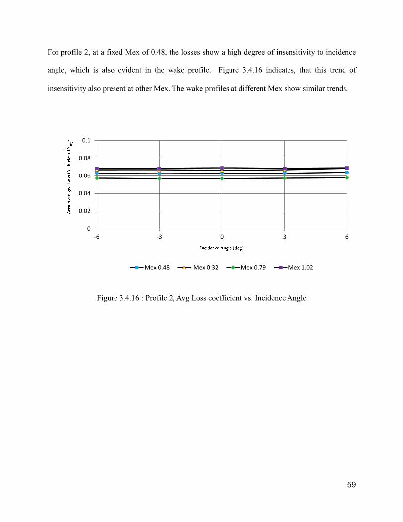
For profile 2, at a fixed Mex of 0.48, the losses show a high degree of insensitivity to incidence
angle, which is also evident in the wake profile. Figure 3.4.16 indicates, that this trend of
insensitivity also present at other Mex. The wake profiles at different Mex show similar trends.
Figure 3.4.16 : Profile 2, Avg Loss coefficient vs. Incidence Angle
0
0.02
0.04
0.06
0.08
0.1
-6 -3 0 3 6
Mex 0.48 Mex 0.32 Mex 0.79 Mex 1.02

60
Figure 3.4.17 : Profile 2, Wake Profile, Mex 0.32
Figure 3.4.18 : Profile 2, Wake Profile, Mex 0.79
0.85
0.9
0.95
1
-1.25 -0.625 0 0.625 1.25
0 deg +3 deg +6 deg -3 deg -6 deg
0.85
0.9
0.95
1
-1.25 -0.625 0 0.625 1.25
0 deg +3 deg +6 deg -3 deg -6 deg
P
S
P
S
SS
SS

61
Figure 3.4.19 : Profile 2, Wake Profile, Mex 1.02
0.8
0.85
0.9
0.95
1
-1.25 -0.625 0 0.625 1.25
0 deg +3 deg +6 deg -3 deg -6 deg
P
S
SS

62
3.5 Comparison between Profile 1 & Profile 2
The test matrix for profile 1 & 2 differ, hence in order to make a good performance comparison of
the two blades, only data for an exit Mach number of 0.48 will be used as this exit Mach number
is common for both blades.
Figure 3.5.1 : Profile 2, Loss comparison between Profile 1 and 2, Mex 0.48
Looking at Figure 3.5.1, the loss coefficient at zero degrees incidence is comparable with the
baseline profile showing only a slight increase in performance over profile 2. Both profiles indicate
that the losses reach a minimum at negative incidences. However, the superiority of profile 2
becomes evident at positive incidence angles, as the losses stay nearly constant with a change in
12 degrees of incidence. Rapid deterioration of performance is seen at positive incidences for
profile 1 and based on this trend, it is expected that the losses will only increase with incidence.
The question arises as to why does profile 1 show a greater degree of sensitivity to losses,
especially at positive incidences, than profile 2.
0
0.02
0.04
0.06
0.08
-6 -3 0 3 6

63
Figure 3.5.2 : Profile 1, Blade Loading, Mex 0.48
0
0.2
0.4
0.6
0.8
0 0.1 0.2 0.3 0.4 0.5 0.6 0.7 0.8 0.9 1

64
Figure 3.5.3 : Profile 2, Blade Loading, Mex 0.48
The above question can easily be answered by looking at Figure 3.5.2 and Figure 3.5.3. The blade
loading at different incidences for profile 2 show very little variation, and that too only towards
leading edge of the SS where rapid acceleration is taking place. The boundary layer growth in the
presence of a favorable pressure gradient is relatively small. In comparison for profile 1, at 0 and
-6 degrees incidence, the blade loadings at the leading edge are similar however, at +6 degrees a
very different trend emerges. On the SS, about 0.1 normalized axial chords, there exists a region
of an adverse pressure gradient which is responsible for accelerating the growth of the boundary
layer. This is primarily the reason as to why the loss coefficient is increasing for profile 1. As the
incidences become increasingly more positive, the adverse pressure in this region will get more
severe leading to a separation on the SS side of the blade.
0
0.2
0.4
0.6
0.8
0 0.1 0.2 0.3 0.4 0.5 0.6 0.7 0.8 0.9 1
65
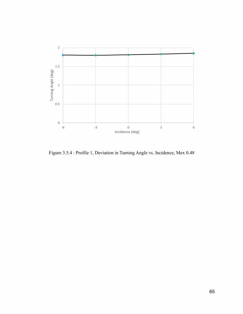
Figure 3.5.4 : Profile 1, Deviation in Turning Angle vs. Incidence, Mex 0.48
0
0.5
1
1.5
2
-6 -3 0 3 6
Turn
ing
An
gle
(deg
)
Incidence (deg)

66
Figure 3.5.5 : Profile 2, Deviation in Turning Angle vs. Incidence, Mex 0.48
Based on Figure 3.5.4 and Figure 3.5.5, it is evident that profile 1 shows a higher degree of
deviation from the exit angle of the blade compared to profile 2. Since the turning angle is
responsible for the output work of a spinning blade, this implies that profile 1 is not as effective at
producing the desired power output in comparison to profile 2.
-0.5
0
0.5
-6 -3 0 3 6
Turn
ing
An
gle
(deg
)
Incidence (deg)

67
3.6 Comparison with Existing Literature
Since experimental results were not available to compare the CFD simulations with, test cases
from other cascade measurements were used to validate the computational results.
Figure 3.6.1 : Loss Coefficient vs. exit Mach number (Song et al) [13]
Data from the above paper shows a similar variation in loss coefficient as a function of exit Mach
number for three different blades. A mass average total pressure loss normalized with respect to
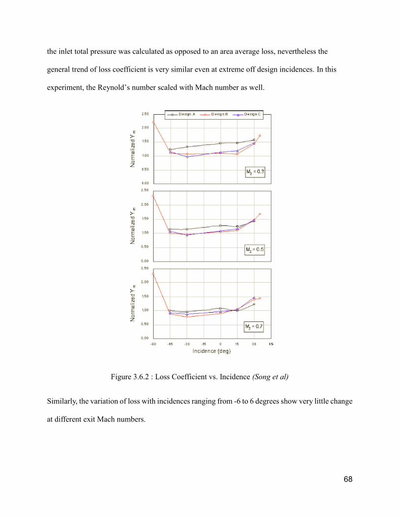
68
the inlet total pressure was calculated as opposed to an area average loss, nevertheless the
general trend of loss coefficient is very similar even at extreme off design incidences. In this
experiment, the Reynold’s number scaled with Mach number as well.
Figure 3.6.2 : Loss Coefficient vs. Incidence (Song et al)
Similarly, the variation of loss with incidences ranging from -6 to 6 degrees show very little change
at different exit Mach numbers.

69
Figure 3.6.3 : Loss coefficient vs. Mex, 0 incidence (Jouni et al)
The data for Figure 3.6.3 was taken from [14]. Comparing the above figure with Figure 3.3.11 and
Figure 3.4.11, the average loss coefficient shows a similar trend with exit Mach number. The
normalizing parameter used in this paper is the incompressible dynamic pressure. Despite this
difference, the trend as well as overall level of losses as well as the trend bear similarity with data
from Profile 1 & 2. As in the previous discussed experiments, the Reynold’s number scaled with
the exit Mach number. The authors in this paper have also noted that the decrease in loss coefficient
with exit Mach number is a result of increase with Reynold’s number.

70
3.7 Conclusions & Future Work
The performance of two high pressure steam turbine airfoils (baseline and mid radius profiles)
were investigated using computational fluid dynamics. Both profiles showed low loss coefficients
as well as a trend of decreasing average loss coefficient vs. exit Mach number. The average loss
coefficient at zero incidence and design exit Mach number of 0.48 were comparable for both
profiles. However, profile 1 showed a steep increase in loss coefficient as the incidence turn
increasingly positive due to the development of an adverse pressure gradient zone towards the
leading edge on the suction side. On the other hand, profile 2 showed little to no variation in losses
over an incidence angle change of 12 degrees (-6 to 6 degrees). Additionally, the profile 1 showed
a higher degree of exit flow deviation in comparison to profile 2, indicating that work extraction
for this airfoil is away from optimal levels. Finally, the change in incidence had no effect on the
exit flow angle for either airfoil. For future work, the loss coefficient at greater off design incidence
angles can be investigated to create a more comprehensive loss bucket. Additionally, an accurate
transition model can be used to investigate the effect of laminar to turbulent change within the
boundary layer and its effects on the overall level and magnitude of losses.

71
4 References
[1] Denton, J. D., 1993, "The 1993 IGTI Scholar Lecture: Loss Mechanisms in Turbomachines,"
Journal of Turbomachinery, 115(4), pp. 621-656.
[2] Brown, L. E., 1972, "Axial Flow Compressor and Turbine Loss Coefficients: A Comparison of
Several Parameters," Journal for Engineering for Power, 94(3), pp. 193-201.
[3] Hoheisel, H., Kiock, R., Lichtfuss, H. J., and Fottner, L., 1987, "Influence of Free-Stream
Turbulence and Blade Pressure Gradient on Boundary Layer and Loss Behavior of Turbine
Cascades," Journal of Turbomachinery, 109(2), p. 210.
[4] Mee, D. J., Baines, N. C., Oldfield, M. L. G., and Dickens, T. E., 1992, "An Examination of
the Contributions to Loss on a Transonic Turbine Blade in Cascade," Journal of turbomachinery,
114(1), p. 155.
[5] Richard, R., 1996, "Transition on turbine blades and cascades at low Reynolds numbers," Fluid
Dynamics Conference, American Institute of Aeronautics and Astronautics.
[6] Brear, M. J., Hodson, H. P., and Harvey, N. W., 2002, "Pressure Surface Separations in Low-
Pressure Turbines---Part 1: Midspan Behavior," Journal of Turbomachinery, 124(3), pp. 393-401.
[7] Li, S. M., Chu, T. L., Yoo, Y. S., and Ng, W. F., 2004, "Transonic and Low Supersonic Flow
Losses of Two Steam Turbine Blades at Large Incidences," Journal of Fluids Engineering, 126(6),
p. 966.
[8] Sanz, W., Gehrer, A., Woisetschläger, J., Forstner, M., Artner, W., and Jericha, H., "Numerical
and experimental investigation of the wake flow downstream of a linear turbine cascade," Proc.
ASME, International Gas Turbine & Aeroengine Congress & Exhibition, 43 rd, Stockholm,
Sweden.

72
[9] El-Batsh, H., 2006, "Numerical study of the flow field through a transonic linear turbine
cascade at design and off-design conditions," Journal of Turbulence, p. N5.
[10] Markus, M., Marco, S., Reinhard, N., and Norbert, H., 2008, "Influence of Inflow Turbulence
on Loss Behavior of Highly Loaded LPT Cascades," 46th AIAA Aerospace Sciences Meeting and
Exhibit, American Institute of Aeronautics and Astronautics.
[11] Abraham, S., Panchal, K., Xue, S., Ekkad, S. V., Ng, W., Brown, B. J., and Malandra, A.,
"Experimental and Numerical Investigations of a Transonic, High Turning Turbine Cascade With
a Divergent Endwall," ASME.
[12] Menter, F., Kuntz, M., and Langtry, R., 2003, "Ten years of industrial experience with the
SST turbulence model," Turbulence, heat and mass transfer, 4, pp. 625-632.
[13] Ng, B. S. W. F., Hofer, J. A. C. D. C., and Siden, G., 2004, "Aerodynamic design and testing
of three low solidity steam turbine nozzle cascades."
[14] Jouini, D. B. M., Sjolander, S. A., and Moustapha, S. H., 2002, "Midspan flow-field
measurements for two transonic linear turbine cascades at off-design conditions," J Turbomach,
124(2), pp. 176-186.

73
5 Appendix
5.1 Profile 1 Mesh Images
Figure 5.1.1 : Profile 1 Mesh
74
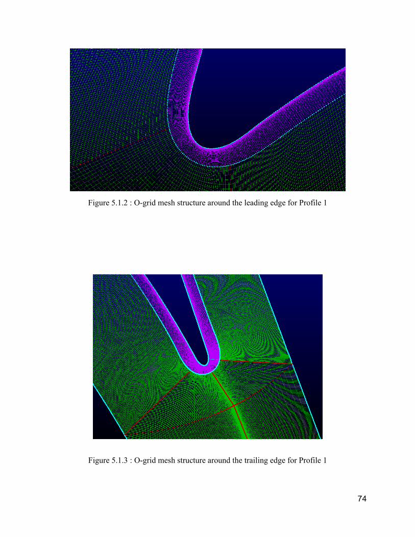
Figure 5.1.2 : O-grid mesh structure around the leading edge for Profile 1
Figure 5.1.3 : O-grid mesh structure around the trailing edge for Profile 1

75
Figure 5.1.4: Mesh Independent grid for profile 1
76
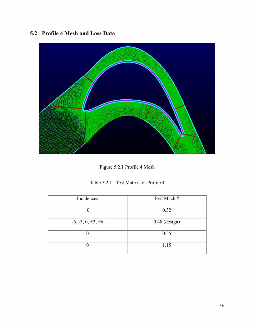
5.2 Profile 4 Mesh and Loss Data
Figure 5.2.1 Profile 4 Mesh
Table 5.2.1 : Test Matrix for Profile 4
Incidences Exit Mach #
0 0.32
-6, -3, 0, +3, +6 0.48 (design)
0 0.55
0 1.15

77
Figure 5.2.2 Profile 4, Blade loading, Mex 0.48, 0° incidence
Figure 5.2.3 : Profile 4, Loss coefficient vs. Mex, 0° incidence
0
0.1
0.2
0.3
0.4
0.5
0.6
0.7
0.8
0 0.2 0.4 0.6 0.8 1
0
0.01
0.02
0.03
0.04
0.05
0.06
0.07
0.08
0.09
0.1
0.25 0.35 0.45 0.55 0.65 0.75 0.85 0.95 1.05 1.15

78
Figure 5.2.4 : Profile 2, Avg Loss coefficient vs. Incidence Angle, Mex 0.48
0
0.01
0.02
0.03
0.04
0.05
0.06
0.07
0.08
0.09
0.1
-6 -4 -2 0 2 4 6

79