pectoral fin control of a biorobotic auv in the dive plane

UNLV Retrospective Theses & Dissertations

1-1-2005

Pectoral fin control of a biorobotic Auv in the dive pLane Pectoral fin control of a biorobotic Auv in the dive pLane

Aditya Simha University of Nevada, Las Vegas

Follow this and additional works at: https://digitalscholarship.unlv.edu/rtds

Repository Citation Repository Citation Simha, Aditya, "Pectoral fin control of a biorobotic Auv in the dive pLane" (2005). UNLV Retrospective Theses & Dissertations. 1803. http://dx.doi.org/10.25669/owxc-gw9x

This Thesis is protected by copyright and/or related rights. It has been brought to you by Digital Scholarship@UNLV with permission from the rights-holder(s). You are free to use this Thesis in any way that is permitted by the copyright and related rights legislation that applies to your use. For other uses you need to obtain permission from the rights-holder(s) directly, unless additional rights are indicated by a Creative Commons license in the record and/or on the work itself. This Thesis has been accepted for inclusion in UNLV Retrospective Theses & Dissertations by an authorized administrator of Digital Scholarship@UNLV. For more information, please contact [email protected].

http://library.unlv.edu/

http://library.unlv.edu/

https://digitalscholarship.unlv.edu/rtds

https://digitalscholarship.unlv.edu/rtds?utm_source=digitalscholarship.unlv.edu%2Frtds%2F1803&utm_medium=PDF&utm_campaign=PDFCoverPages

http://dx.doi.org/10.25669/owxc-gw9x

mailto:[email protected]

PECTORAL FIN CONTROL OF A BIOROBOTIC AUV IN THE DIVE PLANE

bv

Aditya Simha

Bachelor of Engineering Visveswaraiah Technological University, Belgaum. India

2CW2

A thesis submitted in partial fulfillment of the requirements for the

M aster o f Science D egree in Electrical Engineering D epartm ent o f Electrical and Com puter Engineering

Howard R . H ughes College o f Engineering

Graduate College U niversity o f Nevada, Las Vegas

M ay 2005

Reproduced with permission of the copyright owner. Further reproduction prohibited without permission.

UMI Number: 1428590

INFORMATION TO USERS

The quality of this reproduction is dependent upon the quality of the copy

submitted. Broken or indistinct print, colored or poor quality illustrations and

photographs, print bleed-through, substandard margins, and improper

alignment can adversely affect reproduction.

In the unlikely event that the author did not send a complete manuscript

and there are missing pages, these will be noted. Also, if unauthorized

copyright material had to be removed, a note will indicate the deletion.

UMIUMI Microform 1428590

Copyright 2005 by ProQuest Information and Learning Company.

All rights reserved. This microform edition is protected against

unauthorized copying under Title 17, United States Code.

ProQuest Information and Learning Company 300 North Zeeb Road

P.O. Box 1346 Ann Arbor, Ml 48106-1346


ITNTV Thesis ApprovalThe Graduate College University of Nevada, Las Vegas

April 11 .2005

The Thesis prepared by

Aditya Simha

Entitled

"Pectoral Fin Control of a Blorobotlc AUV In the Dive Plane"

is approved in partial fulfillment of the requirements for the degree of

________________ M aster o f S c ien ce In E l e c t r i c a l E n g in eer in g

4-

Examination Comrhijti^ Member

examination Committee Member

Graduate Colle^ Faculty Representative

Examüfàation Committee Chair

Dean of the Graduate College

1017-53 11


ABSTRACT

Pectoral Fin Control o f a B lorobotlc A U V In the D ive P lane

by

Aditya Simha

Dr. Sahjendra N. Singh, Examination Committee Chair Professor of Electrical and Computer Engineering Department

University of Nevada, Las Vegas

Maneuvering of biologically inspired robotic undersea vehicles (BAUVs) is con

sidered in the dive plane using pectoral-like oscillating fins. Firstly, an open-loop

and optimal feedback control system is designed to control a biorobotic AUV in the

dive plane. Next, an inverse control system for dive-plane control is derived based

on a discrete-time AUV model. An approximate minimum phase system with a new

output variable is derived for the purpose of design.

Computational fluid dynamics (CED) is used to parameterize the forces generated

by a mechanical oscillatory flapping foil, which attempts to mimic the pectoral fin

of a fish. Finally, a control system for the independent asymptotic control of the

lateral and rotational motion of a 2-D hydrofoil based on the internal model principle

(servomechanism theory) is derived.

Ill


TABLE OF CONTENTS

ABSTRACT .................................................................................................................... iii

LIST OF F IG U R E S ....................................................................................................... vi

A CKN O W LED GM EN TS.......................................................................................... vii

CHAPTER 1 IN TR O D U C TIO N ...................................................................... 1Biological Classification for M odeling ................................................................. 2Studies C o n d u c te d ................................................................................................. 3Thesis Outline ....................................................................................................... 5

CHAPTER 2 MATHEMATICAL MODEL ..................................................... 10Dive Plane D ynam ics................................................................................................. 10

CHAPTER 3 OPEN LOOP CONTROL ....................................; ................... 15Open-Loop Control System .................................................................................... 15Numerical Results: Open-Loop C o n tro l................................................................. 19

CHAPTER 4 OPTIMAL FEEDBACK CONTROL ........................................ 26Closed-loop Control S y s te m ................................................................................. 26Simulation Results: Closed-loop C o n tr o l ............................................................. 32

CHAPTER 5 INVERSE CONTROL BASED ON CED PARAMETERIZATION 39Fin Force and Moment P aram eterization .......................................................... 39Discrete-time Representation ............................................................................. 43Minimum Phase S y s te m ....................................................................................... 47Inverse Control Law ................................................................................................. 51Simulation R e s u l t s .................................................................................................... 52

CHAPTER 6 CONTROL OF OSCILLATING FOIL FOR PROPULSION . 68Mathematical M o d e l .............................................................................................. 69State Variable Representation.................................................................................. 72Control L a w ............................................................................... 75Observer Design........................................................................................................... 77Simulation R e s u l t s .................................................................................................... 78

CHAPTER 7 CONCLUSION .............................................................................. 84

IV


APPENDIX ...................................................... 86

REFERENCES .......................................................................................................... 87

VITA .............................................................................................................................. 92


LIST OF FIGURES

1.1 A diagram of a fish showing its different f i n s ............................................ 81.2 Different sorts of swimming t y p e s .............................................................. 9

2.1 Schematic of the A U V ................................................................................. 14

3.1 Open-loop control: Determinant of (t) 223.2 Open-loop control: 2 * = 4(m), 16’/ = 40 (rad/sec) .................................. 233.3 Open-loop control: z* — 4(m), wj = 30 (rad/sec) .................................. 243.4 Open-loop control: z* = 2(m), Wf = 30 (rad/sec) .................................. 25

4.1 Feedback control: z* = 2(m), /o — 5(Hz), sampling interval = 0.2 sec 364.2 Feedback control: z* — 2(m), /o = lO(Hz), sampling interval = 0.1 (sec) 374.3 Feedback control: z* = 2(rn), /o = 5 (Hz), sampling interval = 1 (sec) 38

5.1 Spanwise vorticity contours and velocity vectors for flow past the flapping foil ay two different bias angles of 0° and 20°. Note that velocity \ectors are shown on every fourth grid point in either direction. . . . 59

5.2 Fin force and moment for — 0 and 20 (d e g ) ....................................... 605.3 Zeros of the pulse transfer fu n c t io n ........................................................... 615.4 Sinusoidal Trajectory Control Case (Si) ................................................. 635.5 Sinusoidal Trajectory Control Case (S2) ................................................ 645.6 Exponential Trajectory Control (E l) ........................................................ 665.7 Exponential Trajectory Control ( E 2 ) ........................................................ 67

6.1 Spring-driven hydrofo il................................................................................. 806.2 Oscillation Control: Case 1 ........................................................................... 826.3 Oscillation Control: Case 2 ........................................................................... 83

VI

Reproduced witfi permission of tfie copyrigfit owner. Furtfier reproduction profiibited witfiout permission.

ACKNOWLEDGMENTS

This thesis is dedicated to my parents and family. They have always encouraged

me to follow and pursue my dreams, and that is exactly what I have done and will

continue to do.

I would also like to express my immense gratitude to my advisor Dr. Sahjendra

Singh for his tutelage, his time and his wonderful guidance. It has been a pleasure to

have worked under his very able guidance.

I thank Drs. Shahram Latifi. Emma Regentova and Woosoon Yim for kindly

consenting to being a part of my thesis committee.

I would also like to thank several of my peers for their valuable help at several

critical junctions of this thesis.

It would be remiss of me to neglect to thank the staff and personnel of the Electri

cal and Computer Engineering department at UNLV for providing me with excellent

resources and a splendid atmosphere to work in.

VII


CHAPTER 1

INTRODUCTION

Fishes and aquatic mammals are indubitably the denizens of the oceans. These

creatures have evolved over a large period of time and have effectively obtained the

ability to perform swift, intricate and complex manuevers very efficiently, one must

add. In short, they are excellent swimmers. Researchers interested in autonomous

underwater vehicle technology have always been enthusiastic to have the propulsion

for such systems resemble that of the thrust mechanism of actual fish. The reasons

for their unbridled enthusiasm are several: some are listed below:

• Speed: Some species of fish swim at high speeds. This would prove to be very

desirable and an advantage for BAUVs.

• Efhtiency: As mentioned earlier, fish swim with great efficiency. This again

would be beneficial for BAU\”s.

• Maneuverability: Fish have the ability to maneuver themselves into 180 de

gree turns in barely a fraction of their body length [33]. This increases the

maneuverabilitv of BAUVs.


• Stealth Issues: This is especially true when the BAUVs are to be employed for

use by the military. BAUVs are less likely to be detected than conventional

A U V s.

1.1 Biological Classification for Modeling

Most fish swim by utilizing their fins. A diagram showing the different kinds of

fins is shown in Figure 1.1 [34].

Fish are classified into three swimming categories namely anguilloform. ostraci-

iform and carrangiform. A diagram showing the different types of swimmers is shown

in Figure 1.2 [34].

• Anguilloform: These fish are eel-like and possess long thin bodies. They are

very manueverable but unfortunately lack the abilty to swim at rapid speeds.

Therefore, these sorts of swimmers are not considered for modeling in BAUVs.

An example of a fish that is an anguilloform swimmer is the Wolf Eel.

• Ostraciiform: These are large-bodied, slow moving and not very highly efficient

swimmers. These fish have small oscillating fins. An example of a fish that is

an ostraciiform swimmer is the Boxfish.

• Carrangiform: The body is smaller and the thrust is generated by the oscillation

of the rear portion of the body. These swimmers are the most efficient and

swiftest of the three types of swimmers. Therefore, these are the fish that are

the ideal choice to be modeled. An example of this sort of swimmer is the Trout.


1.2 Studies Conducted

Many studies have been carried out on fish morphology, locomotion and applica

tion of biologically-inspired control surfaces to rigid bodies [2-9]. In [2], an ov erview

of the different swimming mechanisms employed by fish is presented. In [9]. the feasi

bility of an oscillating fin propulsion control system as a vehicle actuator is discussed.

This is done by designing and constructing a system and then conducting cruising

tests. A neural network has also been effectively employed. Control systems for

low-speed manuevering of small AUV’s using the dorsal-like and caudal-like fins have

been designed in [7]; a hydrodynamic control scheme was designed here.

Several studies have been carried out so as to measure forces and moments pro

duced by oscillating fins in laboratory settings [6,7, 10-12]. Kato in his work [10] has

presented work on mechanical pectoral fins with an emphasis on their applicability

to AUV’s. In his earlier work [11], Kato used fuzzy control to guide and manuever a

robotic fish equipped with two-motor-driven mechanical pectoral fins. From [11.12].

it has been observed that pectoral fins undergoing a combination of lead-lag. feather

ing and flapping motion have the ability to produce large lifts, side forces and thrust

which can then be used to control and propell .AUV’s. Computational methods have

also been utlized to obtain forces and moments of flapping and pitching foils [16.18].

These experimental and numerical results provide forces produced by the fins for

only a set of motion patterns of oscillating fins. .A.n analytical representation of the

unsteady hydrodynamics of oscillating foil have been obtained using Theodorsen's

theory [14]. Finite dimensional models are extremely interesting from the point of


view of control system design. Because analytical representation of forces is extremely

complicated, neural networks and fuzzy controllers have been suggested for controller

design [10-12]. Of course, the designer must have sufficient knowledge of the effect of

fin forces on the vehicle to develop rule-based logic for the control of AUVs. In a recent

paper, the design of open-loop and closed-loop control systems of a biorobotic AUV

for the set-point regulation in the dive plane using optimal control theory has been

considered [19]. However, for agility in maneuvering, it is essential to design control

systems for following time-varying trajectories. For time-varying trajectory control,

the inversion (decoupling) control technique provides a valuable tool. Considerable

research has been done in this important area [20-22]. However for exact output

trajectory control, the system must be minimum phase; that is, its zero dynamics

must be stable. The zero dynamics of a system represent the residual motion of the

closed-loop system including the inverse control law when the output is constrained

to be zero. For nonminimum phase systems, inverse controller cannot be synthesized

because in the closed-loop system, the residual motion diverges. For nonminimum

phase systems, approximate trajectory control can be accomplished by constructing a

modified output such tha t the new system is minimum phase [22]. For linear systems,

one obtains a modified minimum phase system by eliminating the unstable zeros of

the original transfer function and then performs inverse control law design [7. 23].

Such an approach has been used for the dorsal fin control of a continuous-time model

of an undersea vehicle [7].

Considerable research is available in literature for the design of control systems for


undersea vehicles. These conventional controllers use continuously deflecting control

surfaces for maneuvering. Fish produce propulsive and maneuvering forces and mo

ments by flapping their fins. Oscillating fins produce periodic forces. Therefore, for

fish-like control of BAUVs, it is of interest to develop control algorithms which are

based on oscillatory (periodic) control forces.

1.3 Thesis Outline

The contribution of this thesis is outlined in this section. Control systems for the

dive plane maneuvering of biorobotic AUVs using pectoral fins are designed. These

pectoral fins produce a variety of periodic forces and moments which have wide range

of harmonic functions depending on the oscillation mode and oscillation parameters

of the fins. It is essential to capture their basic features which simplifies controller

design. For this purpose, characterization of these periodic forces using Fourier series

is very attractive. These Fourier coefficients play an important role in the design

of the control systems in this paper. Two kinds of control laws (an open-loop and

a closed-loop) for maneuvering are derived in the third and fourth chapters of this

thesis. For the open-loop control, an analytical solution for the Fourier-coefficients

is derived for a given maneuver. The derived coefficients in turn determine the re

quired fin forces and moments for the maneuver of the vehicle. It is seen that for

a given maneuver there exist multiple solutions for the pectoral force and moment.

This flexibility can be exploited to satisfy certain given performance criteria. The

second control system uses state variable feedback for synthesis. For the closed-loop


control, the bias angle is utilized as the control input. For the purpose of control,

the bias angle is switched to new values at the chosen sampling instants which are

integer multiple of the fundamental time period of the fin force and moment. An

integral feedback is included in the control law for the precise depth control. In

the open-loop control scheme, the pectoral fins complete the maneuverby operating

in a fixed oscillation mode with constant oscillation parameters. However, for each

maneuver one needs to compute the motion pattern separately. Simulation results

using the open-loop and closed-loop control systems are obtained for the dive plane

control. In the fifth chapter, a Fourier series expansion of the forces and moments

produced by the pectoral fins based on data obtained from computational fluid dy

namics (CFD) is derived. A discrete-time model of the .AUVs then derived for the

purpose of design. However it turns out that the AUV model is nonminimum phase

(the transfer function relating the output (depth) and input (bias angle) has unstable

zeros), and therefore one cannot design an inverse control system for exact tracking

of the output trajectory. It is found that the number of unstable zeros is a function

of the location of the pectoral fins on the BAUV. To overcome the obstruction cre

ated by unstable zeros, an approximate discrete-time system (which depends on the

fin location) is obtained by essentially eliminating the unstable zeros from the pulse

transfer function. .An analytical expression of the output matrix of the approximate

minimum phase system is derived. Then an inverse control law is derived for the

control of the new output variable. Interestingly, the controller designed based on

the new output variable, accomplishes accurate trajectory following of the prescribed


depth trajectory. Simulation results show good tracking of time-varying (exponential

and sinusoidal) reference depth trajectories. Furthermore, the pitch angle response is

stable. It is noted that the methodology developed here differs from the conventional

approaches in which control surfaces are continuously deflected for control. Here oscil

lating fins are used for flsh-like maneuvers of BAUVs. In the sixth chapter, a control

system for the independent asymptotic control of the lateral and rotational motion

of a 2-D hydrofoil based on the internal model principle (servomechanism theory) is

derived. The foil is spring driven by two actuating signals and it experiences lateral

displacement and the angular rotation in the free stream. The foil model includes

hydrodynamic forces computed using the theory of unsteady aerodynamics. A com

mand generator is used to generate specified command trajectories which are linear

combinations of sinusoidal functions of distinct frequencies, amplitudes, phase angles

and average values. A feedback control law is designed so that plunge displacement

and pitch angle of the foil asymptotically tracks the command trajectories generated

by the command generator. The control system includes a servocompensator which

is fed by the lateral and rotational trajectory errors. Since the states associated

with the Theodorsen function cannot be measured, an observer is designed to obtain

the estimates of the unavailable states. Then the controller is synthesized using the

estimated state variables. Simulation results are presented which show that in the

closed-loop system, independent asymptotic control of the plunge displacement and

pitch angle trajectories are accomplished.


m Ë lm \

.....

Figure 1.1; A diagram of a fish showing its different fins


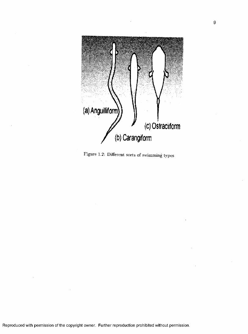
Figure 1.2; Different sorts of swimming types


CHAPTER 2

MATHEMATICAL MODEL

In this chapter, the mathematical model used in three chapters of this thesis is pre

sented. The model used in chapters 3,4 and 5 is presented in this chapter, while the

model followed in chapter 6 is presented in that chapter itself.

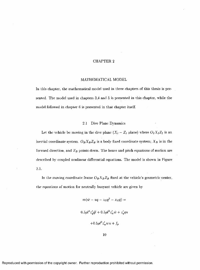
2.1 Dive Plane Dynamics

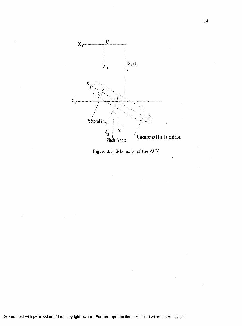
Let the vehicle be moving in the dive plane {Xj — Z; plane) where O iX jZ j is an

inertial coordinate system. OgAgZg is a body fixed coordinate system; X b is in the

forward direction, and Zb points down. The heave and pitch equations of motion are

described by coupled nonlinear differential equations. The model is shown in Figure

2 . 1 .

In the moving coordinate frame OgAgZg fixed at the vehicle’s geometric center,

the equations of motion for neutrally buoyant vehicle are given by

m.{w — uq — zgQ - xcq) =

O.opl^z'^ql + O.dpl^z'^ii; -t- z'^qu

+0.5pl^ z'^wu + fp

10


11

lyQ 4- m z c i û ■+ w q ) — m x c i w — uq) =

+0.bpl^Ml,wu — xgb^V cos 6 - zgb^V sin 6 + rup

z = —usinO + w cos 6 (2 .1)

where 6 is the pitch angle, q — 0 , x g b = x g — z g , Z g b — z g - z g , / = body length, p

— density, w is the velocity along the Zg-axis, and z is the depth, fp and rrtp denote

the force and moment produced by the pectoral fins. Here X g , Z g and X b , Z g are

the coordinates of the center of gravity and the center of buoyancy, respectively. It is

assumed that Og is at the center of buoyancy and the forward velocity is held steady

( u = U) by a control mechanism.

In this study, only small maneuvers of the vehicle are considered. As such lin

earizing the equations of motion about u,' = 0, g = 0, z — 0 and 6 = 0, one obtains

m - z,û -m xG - Zg 0

~?nxG - l y - Mg 0 g

0 0 1 z

r 1 r 1

z^.U Zg -f mU 0

MyjU Mg — TUXgU 0

1 0 0

It;

0 fp

-f — G'gH 6 + rrtp

- U 0

(2 .2)


12

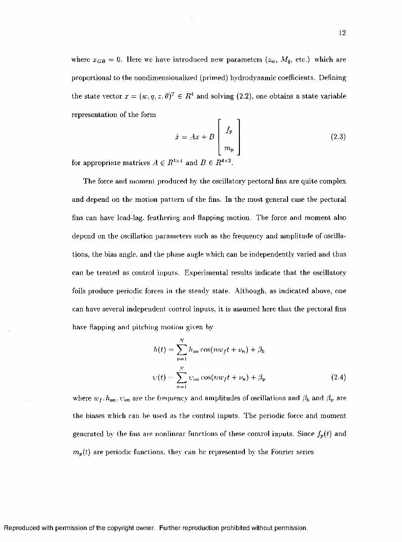
where xgb — 0. Here we have introduced new parameters {zy,, M ,, etc.) which are

proportional to the nondimensionalized (primed) hydrodynamic coefficients. Defining

the state vector x = {w, q, z, 0)' e and solving (2.2), one obtains a state variable

representation of the form

uX = -4.T + D

TUp(2 .21)

for appropriate matrices A e R^'^^ and D £ R^^^.

The force and moment produced by the oscillatory pectoral fins are quite complex

and depend on the motion pattern of the fins. In the most general case the pectoral

fins can have lead-lag, feathering and flapping motion. The force and moment also

depend on the oscillation parameters such as the frequency and amplitude of oscilla

tions, the bias angle, and the phase angle which can be independently varied and thus

can be treated as control inputs. Experimental results indicate tha t the oscillatory

foils produce periodic forces in the steady state. Although, as indicated above, one

can have several independent control inputs, it is assumed here that the pectoral fins

have flapping and pitching motion gi\en by

Vh(t) = ^ hon cos{nwft + iz„) + j3h

n=\A*

v{t) = ^ ÇV;, cos{muft -f 1/n) + fSy, (2.4)r7=l

where iCf. hon, are the frequency and amplitudes of oscillations and [3h and ,3 are

the biases which can be used as the control inputs. The periodic force and moment

generated by the fins are nonlinear functions of these control inputs. Since fp{t) and

mp(t) are periodic functions, they can be represented by the Fourier series


13

Mf p = sm{nwft) + f e r , cos{nWft))

n=0

MTUp = ^ ( r r ïs n sm{mvft) + cos{nWft)) (2.5)

n= 0

where it is assumed that the fin produces dominant M harmonically related compo

nents and the harmonics of higher frequencies are negligible. The Fourier coefficients

fij and rriij capture the characteristics of the time-varying signals fp{t) and mp{t) and

play a key role in the design of control systems for maneuvering.


14

X 0

X, I t .

Depth7.

Pectoral Fin

Z , I, 'Circular to Flat Transition

Pilch Angle

Figure 2.1: Schematic of the AUV


CHAPTER 3

OPEN LOOP CONTROL

In this chapter, an open loop control system is designed to control a biorobotic AUV

in the dive plane. This is done by using oscillating pectoral fins. This control system

is presented here in this chapter by using the periodic forces and moments generated

by the pectoral fins. The mathematical model which is followed here has already been

presented in the preceding chapter.

3.1 Open-Loop Control System

In this section, the design of the open-loop controller is considered. Let the initial

condition be z(0) = zq and suppose that it is desired to steer the vehicle to the

terminal state z* = (0,0, z*,0)^ , where z* denotes the desired input. For simplicity

in presentation, we assume that only the first and second harmonics are present in

the following equation

M

f p = s m { n w f t ) + f e n c o s { n W f t ) )r i= 0

M

m.^77 = 0

.p = s i n { n w f t ) + m e n < t o s { n i v j t ) )

15


16

Then (2.5) gives

fp 1 sin wft cos wft sin 2wft cos 2wft

= (t)^{t)pf

rrip = (t> {t)pm.

Pf

(3.1)

where the vector function 0(f) E is

1 sin wft cos wft sin 2wft cos 2wft

and the vector of the Fourier coefficients are

Pf = fcO / s i / c l f s 2 fc 2 e

P m ■nico rrisi rrici m^2 '"ic2

are the constant parameters. Now for steering the vehicle from the initial condition

Xq to X*, we shall find appropriate values of the vectors pf and Pm associated with

the fin force and moment. The solution of (2.3) and (3.1) can be written as

x{t) = e''’*ZoJo

where p = (p j,p ^ )^ € is a constant vector and

(3.2)

0 (f)0^(f) 0

E R 2x10

0 0:«(f)

and 0 denotes null matrices of appropriate dimensions. Define

A"o(f) = c xo


17

Z ( f )= re^('-^ )B 0(T )dT (3.3)Jo

Then Vo(f) G and Z{t) G can be obtained by solving the differential equa

tions

-Vo(f) = AA'’o(f), Vo(0) = X q ,

Z(f) = AZ(f) 4- B 0(f), Z(0) = 0 (3.4)

For the transfer of xq to x* at the instant t* > 0, using (3.2) and (3.3), one must have

z ' = Ao(<*) + Z (f')P (3.5)

For the existence of solution of (3.5), x* — Ao(f*) must be in the range space of Z{t*).

Since zq is arbitrary, (3.5) can be solved for p if rank {Z{t*)} = 4. Noting that (3.5)

does not have a unique solution, an optimal value of p can be obtained by minimizing

an appropriate quadratic function

J = p^W p

where IF is a symmetric positive definitive weighting matrix. By the choice of IF, one

can obtain suitable values of the vector p. Then the unique solution for p obtained

by minimizing J can be shown to be

p* = H /'-^ z:^ (r)(z(r)H '-'z^ (r))-X z* - %o(r)) (3.6)

One notes tha t a general solution of (3.5) can be written as

p = p* + q (3.7)


18

where q e N{Z{t*)), the null space of Z{t*). Indeed the pectoral fin forces and

moment for which the Fourier coefficients q belong to the null space of Z{t*) do not

contribute to the transfer of Xq to x *.

To this end, it is appropriate to discuss, the question related to the synthesis

of the desired control law. It is pointed out that the rank of Z{t*) depends not

only on the pectoral fin oscillation mode and oscillation parameters, but also on the

choice of the transfer interval [O.t*]. Because, the forcing function in the Z-dynamics

is consisting of sinusoidal signals, Z{t) is sinusoidal and the determinant A of

Z{t)Z^ (t) is is an oscillatory function of time. One can select any value of t*, such

that A{t*) yields a feasible p* associated with the pectoral fin motion. Since, pectoral

fins can have a variety of motions, they have the capability to generate forces and

moments yielding a set of p large enough which contains p*. The Fourier coefficients

are functions of the oscillation parameters and belong to certain bounded intervals.

As such, one can use constrained optimization algorithms to obtain solution of (3.5)

with inequality constraints on the Fourier coefficients. According to the following

equation,

Mfv = sm{nwft) + fcnCOs{nWft))

n=0

MTrip = ^ ( m s „ sm{nwft) + rricn cos{nwft))

n =0

the dimension of the design-parameter vector p = (py increases if additional

sinusoidal components in the fin force and moment are included. Fin forces consisting

of larger number of harmonic terms by the choice of M in (2.4) which is as follows


19

Nh{t) = cos{nwft + Ur,) + (3h

n = l

N-Ipit) = ^ 'Ipon COs{nWft + Un) +

n = l

provide fiexibility in satisfying (3.5) which can be exploited to satisfy certain response

characteristics of the dive-plane control system. It is also pointed out tha t the design

approach presented in this section is equally applicable if the fin motion is not periodic.

3.2 Numerical Results: Open-Loop Control

In this section simulation results for the svstem

X = Ax + Bfv

with the open-loop control law (3.1) and (3.7) using p — p* with W = I are presented

(7 denotes an identity matrix). The model parameters for simulation of the vehicle

are taken from [7j. It is assumed that the vehicle is initially moving horizontally

at a constant speed U = 3 (m/s) and the initial condition is x(0) = (0,0,0,0)^ .

The desired state at t* is selected as x* = (0, 0, z*, 0)^. That is, one would like to

maneuver the vehicle such that at t = t*. the vehicle dives down to a depth of z* and

subsequently moves horizontally.

C ase 1: Open-loop control: z* = A (m), t* = 20 (s), wj = 40 (rad/s)

It is desired to maneuver in t* = 20 seconds and z* is taken to be 4 (m). The

frequency wj is chosen as wj = 40 (rad/sec). Thus fp contains sinusoidal terms


20

of frequencies 40 and 80 (rad/s). Of course it is assumed that the fin motion in

(2.4) is suitably chosen to yield fin force of the form indicated. Although the control

system of the previous section is applicable to any general case, for the purpose of

illustration, we assumed here a restricted case in which nip = 0.25fp, tha t is fp and

nip are linearly related. Such situations do arise for certain oscillation patters of the

fins. It is noted that by the choice of linearly related moment and force, one has fewer

elements in the control parameter vector p (p = py € Pm = 0.25py) to satisfy

(3.5) for maneuvering the vehicle; however, it is found that in spite of this limitation,

several solutions for p still exist and maneuver can be completed.

The simulated responses are as shown in Figs. 3.1 and 3.2. The plot of the

determinant A(t) of {Z{f)Z{t)^ ) is shown in the Fig. 3.1. It is seen tha t A(f) is

oscillatory and for the chosen wj, one can select any t* > 12 (sec) for maneuvering

as long as A(f*) 0.

Fig. 3.2 shows smooth convergence of the depth trajectory to the desired value

(4 (m)) in the chosen time interval of 20 seconds. During this interval of time one

observes an oscillation of extremely small amplitude superimposed on the mean pitch

angle trajectory. The pitch rate and pitch angles are also have oscillatory motion.

However, it is pointed out that the initial state x(0) = 0 is precisely steered to the

chosen state x* = (0,0,4,0)^ at t = 20 (sec). Indeed if the fin force and moment

are set to zero beyond 20 (sec), the vehicle continues to move along the horizontal

path (The plots beyond 20 (sec) are not shown here). Oscillatory fin force fp (shown

only over t € [0.1.5] (sec) for clarity) of magnitude less than 50 (N) is required for


21

the maneuver. The pitch angle swings between —5 and 0 degrees. The maximum

magnitude of the velocity w remains within 0.08 (m/s) which is quite small. The

pitch rate is also small (less than 15 (deg/sec). We observe small nonzero average

values of the pitch rate and the velocity w.

C ase 2 Open-loop Control: z* — 4 (m), t* — 20 (s), Wf — 30 (rad/s).

Simulation is done using a lower value of Wf but the remaining conditions of Case

1 are retained. The responses are shown in Fig. 3.3.

We observe that the vehicle smoothly attains the desired depth as well as the

terminal state, at 20 seconds. The pitch angle is between —5 and 0 degrees. The

maximum magnitude of the normal force is less than 20 N. The velocity stays between

—0.06 to about 0.035 (m/s). It is seen that for lower frequency of oscillation the

magnitude of the normal force is smaller. Of course, one can obtain different normal

force history for the maneuver by selecting the weighting matrix W ^ I.

C ase 3 Open-loop Control: z* == 2 (m), t* = 20 (s), Wf — 30 (rad/s).

The simulation is done by retaining the conditions of Case 2. But a smaller terminal

depth z* = 2 (m) for control is chosen. The responses are as shown in Fig. 3.4.

The desired depth and terminal state are reached at 20 seconds. The pitch angle

varies between —2.5 and 0 degrees. The normal force is less than 10 N which is

almost half of that required for Case 2. The maximum velocity is only slightly over

0.03 (m/sec) and the pitch rate is less than 4.5 (deg/sec). Thus it is seen that smaller

commands for maneuver can be chosen to reduce the magnitudes of state trajectories

and the control input in the transient period.


22

C(Cc

1V.B0 Û

30

20

10

0

-100 5 10 15

Time(sec)20

Figure 3.1; Open-loop control: Determinant of Z{t)Z^'{t)


23

20

( ' ' ; '

Timelsec)5 10 15 20

TanefsecJ

5 10 15Time (sec)

Figure 3.2: Open-loop control: z* = 4(m), wj = 40 (rad/sec)


24

20

a-0.04

5 10 15Tim^sec)

5 10 15 20Time(sec|

0 5 10 15 20Time (sec)

Figure 3.3: Open-loop control: z* = 4(m), wj = 30 (rad/sec)


25

2 -5 ,

20

5 -0.02

5 10 15

Timeisec:'5 10 15T (ssc)

0 5 10 15 20Time (sec)

Figure 3.4; Open-loop control: z* = 2(m), wj = 30 (rad/sec)


CHAPTER 4

OPTIMAL FEEDBACK CONTROL

In this chapter, an optimal feedback control system is designed to control a biorobotic

AUV in the dive plane. This is done by using oscillating pectoral fins. This control

system is presented here in this chapter by using the periodic forces and moments

generated by the pectoral fins. The mathematical model used here has been presented

in the second chapter.

4.1 Closed-loop Control System

In this section, the design of a feedback dive-plane control law is considered. Unlike

the open-loop control system of the previous chapter, in which pectoral fins have a

fixed motion pattern, here it is assumed that there are control variables which can

be altered periodically. Although, one can chose a variety of oscillation parameters

such as the amplitudes and frequency of oscillation and phase and bias angles, for

simplicity in presentation, we assume that only the bias angles 3 — 3w is varied

periodically and 3h = ^ and the remaining oscillation parameters are constant.

It has been experimentally shown that the mean value of the normal force and

the pitching moment varies almost linearly with 3 [5] and the amplitude of fin force

26


27

and moment are functions of /?.

Expanding the fin force and moment in a Taylor series about = 0 gives:

f p { t , 3 ) — /p(U 0) + 0),J + 0 { 3 ^ )

mp{t , 3 ) = rupit, 0) + 0)/3 + 0 { 3 ^ ) (4.1)

where 0{3^) denotes higher order terms. We assume here that for a fixed /? 6 iî,

f p { t + T o , 3 ) = /p(U 3 ) and mp(t+To, 3 ) = fnp{t, 3): t > 0 (Tq denotes the fundamental

period). Then the partial derivatives of fp and rup with respect to 3 are also periodic

functions of time. Then using the following equation

M

fp = Slli{nWft) + fen cos{nwft))n=0

M

m.p — y^frrisn sm{nwft) + rricn cos{nWft))n=0

and (4.1), one can approximately express fp and nip as

M

fp = Y 2 fsn (0) sin nw / t + /c„ ( 0) cos nwjt+n=0

M

X ] ( ^ ^ ( 0 ) sin nwft + ^ ^ ( 0 ) cos 7iWft)3n —O

M

nip nisn{{f) sin nWft + nicr,(0) cos rnrft+n = 0

(0) sin nwft + {0) cos nir jf) 3 (4.2)

where 0{3^) terms are ignored in the series expansion. For simplicity in presentation,

we assumed that M — 2 similar to the previous chapter. We define


28

A = (/co(o), A i(0): A i(0), A 2(0) , / ^ ( 0))^

nia - (m^o(0) ,m^ , i (0) ,mci(0) ,ms2(0 ) ,mc2(0 ))^

Then using (4.2) and (4.3), we get

fp{t) = 0^(A + 3 h )

mp{t) = 4> {ma + 3mb) (4.4)

and the dive plane dynamics take the form

z = + B $(f)A + B$(t)A/3 (4.5)

where

jFc = (jr;r,ml) E fz" (4.6)

For the purpose of control, the bias angle is periodically changed at a sampling interval

of T* where T* is an integer multiple of the period To, i.e., T* = tioTq. where //q is

a positive integer. This way one switches the bias angle at an uniform rate of T*


29

seconds at the end of no cycles. For the derivation of the control law, the transients

introduced due to switching are ignored in this study. Since the bias is changed

periodically, it will be convenient to express the continuous-time system (4.5) as a

discrete-time system. The function /3(t) now has piecewise constant values 3k for

t 6 [kT*. {k 4- l)T*), k — 0,1, 2 The solution of (4.5) is given by

T(f) = + r e^(*-*")B$(T)[A + A/3(T)]dT (4.7)Jto

Taking to = kT*, and t — {k + 1)T*, one has

x[{k + l)T*] = x{kT*)T

r{k+OT'/ + (4.8)

JkT*

since 3{t) = 3 k , t e [kT*, {k + 1)T ')

Let {k + 1)T* — T = s. Then noting that

$ ((A ;-H )r * -g ) = $ ( -a ) (4.9)

(4.8) gives

x[{k + 1)T*] = x(kT*)+

/ + Îv3k]dsJo

= Adjr(Ar') -b (4.10)

where Ad ~ and Bd = e"^^jB$(—s)ds. For the precise depth control, it is

desirable to include a feedback term in the control law which is proportional to the


30

integral of the depth tracking error.For this, a new state variable Xg is introduced

which satisfies

+ i ) r ] = z* - + z / t r ) (4 .1 1 )

where z* — y{kT*) is the tracking error,

= z(AT') = C T (& r )

and C = [0,0,1,0].

Defining the augmented state vector Xa as

the system (4.10) and (4.11) is written as

%.[(& + i)r] = A , 0 z(AT*)

- C 1 z / t r * )+

B d f v

3 k +0 2*

(4.12)

= A .z .(tT ') + + da (4.13)

where the constant matrices Aa, Ba and da are defined in (4.13).

The control of the system (4.13) can be accomplished by following the servomech

anism design approach in which da is treated as a constant disturbance input. The

design is easily completed by computing a feedback control law of the form

3{kT*) = -K xa ikT *) , Â: = 0,1,2,... (4.14)


31

where K is a constant row vector such tha t the closed-loop matrix

Ac = (Aa - BaK)

is stable. It is well known that that one can assign the eigenvalues of Ac arbitrarily

if (Aa, Ba) is controllable [16-18]. For the discrete-time system, this implies tha t one

must choose K such tha t the eigen-values of Ac are strictly within a unit disk in the

complex plane. In this study, an appropriate value of K is obtained by using the

linear quadratic optimal control theory. For this one chooses a performance index of

the formOO

A = ^ z ^ ' ( t r ) Q z . ( A T 3 -b (4.15)fc=0

where Q is a positive definite symmetric matrix and p > 0. The optimal control law

is obtained by minimizing Jo for the system

z .[ ( t -b l ) r ] = A .z(;rT') -b (4.16)

The system (4.16) is obtained by setting — 0 in (4.13). The feedback matrix K is

obtained by solving the discrete Ricaati equation [18]

P = Q + A lP A . - A lP B .(p -b P r P B a )B lP A . (4.17)

and then setting the feedback matrix as

R: = - ( p -b (4.18)

The choice of the weighting matrix Q and the parameter p is made to obtain desirable

responses and the convergence of the tracking error to zero.


32

To this end, a discussion of the two designed control systems is appropriate. We

note that the open-loop controller of the previous chapter does not require any change

in the motion pattern of the pectoral fins. For the open-loop control scheme, the

Fourier coefficient associated with fin force and moment are determined. It is essential

that these coefficients lie in the feasible parameter set Q obtained by certain choice

of motion pattern and oscillation parameters of the pectoral fins. For the feedback

control system designed in this chapter, the bias angle is periodically varied and

kept constant over the selected sampling period T* = noTo. The pectoral fin must

produce force and moment such that the controllability condition is satisfied. The

choice of the sampling period also provides flexibility in meeting the controllability

condition. The synthesis of the feedback control law requires measurement of all the

state variables, and switching of the bias angles by the actuator. However closed-loop

system can provide robustness to parameter uncertainty compared to the open-loop

control system. The closed-loop system provides asymptotic regulation of the tracking

error. But open-loop control law can complete maneuver in a finite specified time.

As such one can use a dual mode control synthesis for depth control in which one

first uses the opemloop control law and then switches to the feedback law for precise

regulation in the vicinity of the terminal state.

4.2 Simulation Results: Closed-loop Control

In this section, the feedback discrete control law (4.14) is simulated. For the op

timal control law design, the performance index Jo with Q = diag{l, 1500,1.1000,1)


33

and y — 400 is chosen. The bias angle is changed to a new value every T* = tioTq

seconds where To = ^ is the fundamental period of fp and nip.

For the purposes of illustration, it is assumed that fp and nip have only fun

damental components, and therefore it is assumed that A 2 , A2 , are zero.

Experimental results indicate that for zero bias angle, the mean values of fp and nip

are zero. Therefore the vectors A , A, '^a, and mb are selected as

A = (0,5,8), A = (20,30,36)

n ia = (0,1.5,3.2), mb = (10,12,9)

However, it is pointed out that the derived controller is effective even when the

mean values are nonzero. The initial conditions and the terminal state are chosen as

z(0) = (0,0,0,0)^ and x* = (0,0,2,0)^ with z* — 2 (m). Thus one desires to move

to a depth of 2 (m).

C ase 1 Closed-loop control: frequency A = 5 Hz, T* = To

The closed-loop system (2.3)

X = Ax 4- DATTlp

including the discrete control law (4.14) is simulated. The frequency of oscillation is

A = 5 (Hz) and the sampling period is T* — Tq = 0.2 (sec). That is, the bias angle

is updated every cycle. The simulated responses are shown in Fig. 4.1.

A smooth regulation of the depth trajectory to the desired value of 2 (m) is

accomplished. The response time is of the order of 10 seconds. The oscillatory


34

normal force and moment are within 10 (N) and 4 (Nm), respectively. It is observed

that the pitch angle response has oscillations of tiny amplitude superimposed over a

smooth mean motion. It is pointed out that these tiny oscillations of the pitch angle

persist even in the steady-state. However, it is interesting to note that this minor

pitching motion causes no problem. The vehicle continues to move horizontally and

the perturbations in the depth trajectory between the sampling instants due to the

pitching action of the vehicle are hardly noticeable. The piecewise constant bias angle

remains within 2 (deg).

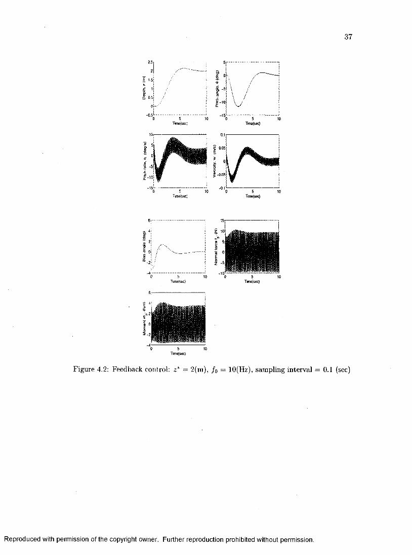
C ase 2 Closed-loop control: A = 10 (Hz), T* = To

It is assumed that the fins are oscillating with a higher frequency 10 (Hz) (twice

of that used in Case 1) and the sampling period is T* — To = 0.1 (Sec).

It is seen that precise control of the depth of the vehicle is obtained (Fig. 4.2)

and compared to the Case 1, one has a smaller tracking error at t = 10 (sec). This

is expected since the bias angle is updated at a faster rate compared to Case 1.

The responses remain close to those of Case 1, and the fin force and moment have

magnitudes of similar order. The bias angle magnitude is only slightly higher in this

case. The tiny oscillations in the pitch trajectory observed for lower frequency in

Fig. 4.2 have almost disappeared. Thus it seems tha t the choice of fins oscillating at

higher frequencies is preferable.

C ase 3 Closed-loop control: f — 5 (Hz), T* = 5Tq second Here, the frequency of

oscillation is retained at A — 5 (Hz) similar to Case 1. but a slower sampling rate of

value T* = 5Tq = 1 (sec) is assumed.


35

Thus now unlike Case 1, the bias angle switches to new values at the interval of

one second instead of 0.2 (sec). We observed that compared to Case 1, the response

time (20 seconds) has almost doubled (Fig. 4.3). But the fin force and moment have

magnitudes of similar order. It is seen that initially the depth trajectory has a slight

overshoot in the wrong direction (upward motion) but recovers and dives down to

attain the desired depth. Apparently, slower sampling rate has a detrimental eflFect

on the maneuverability of the vehicle, but this may not be avoidable, especially when

the actuators are slower.


36

2.5

& 1.5

0,5

-0.5

5 10Time(s@c)

"'^O 5 10 '*” o 5 II

5 10TCT>e(sec)Tenesec)

Figure 4.1: Feedback control: z* = 2(m), /o = 5(Hz), sampling interval = 0.2 sec


37

2,5

0.5

-G.55 10

Twn sec)

î:

5 10uîneisec) 5 10T»ne(sec)

5Time(sec)

Figure 4.2: Feedback control: z* — 2(m), /o — lO(Hz), sampling interval = 0.1 (sec)


38

2.5

I 15

0.5

20

0.05.?

0 5 10 15 20 Q 5 10 15 20TImelsec? Time(sec)

0.2

- 0.4

-0 6

0 5 10 15 20 0 5 10 15 20Tifneiseci

Time(sec)

Figure 4.3: Feedback control: z* = 2(m), / o = 5 (Hz), sampling interval = 1 (sec)


CHAPTER 5

INVERSE CONTROL BASED ON CED PARAMETERIZATION

In this chapter, an inverse control design is derived based on a discrete-time AUV

model. Computational fluid dynamics (CED) is used to parameterize the forces gen

erated by a mechanical flapping foil which attempts to mimic the pectoral fin of a

fish. The mathematical model used here has been presented in the second chapter.

5.1 Ein Eorce and Moment Parameterization

It is assumed that the BAUV model has one pair of pectoral fins that are arranged

symmetrically around the body of the AU\’. Eigure 2.1 shows a schematic of a typical

AUV. Each fin is assumed to undergo a combined pitch-and-heave motion described

as follows:

h{t) = /i] sin(a;/-t) (5.1)

fpit) = 13 + Vi sm{iOft 4- zvi) (5.2)

where h and ijj correspond to the heave motion and pitch angle, respectively; and the

pitching is assumed to occur about the center-chord location. Furthermore, Wf,

are the frequencies and amplitudes of oscillations. 3 , is pitch bias angle and is the

phase difference between the pitching and heaving motions.

39


40

As a result of this flapping motion, each fin experiences a time varying hydro-

dynamic force (which can be resolved into a thrust component and a lift (or pitch)

component fp ) and a pitching moment nip. The hydrodynamic forces on the pectoral

fin also produce rolling, and yawing moments on the BAUV which affect its dynamics.

However, since dive-plane dynamics and maneuvering is assumed to be affected by

the pitching force and moment only, we limit our discussion to these components.

Since fp{t) and mp{t) are periodic functions, they can be represented by the Fourier

seriesM

fp = sm{nwft) 4- cos(nu!/t))71=0

Mnip = ^ (m ® sm{nwft) 4- cos{nWft)) (5.3)

n = 0

where it is assumed that the fins produce dominant M harmonically related compo

nents and the harmonics of higher frequencies are negligible. The Fourier coefficients

/ “ and m“ , a G {s, c}, capture the characteristics of the time-varying signals fp{t) and

nip(t). Parameterization of these coefficients is therefore needed in order to complete

the equations that govern the motion of the BAUV in the dive plane.

The following are the key non-dimensional parameters that govern the perfor

mance of a rigid, rectangular, flapping foil: Re, St, Vi, t'l, fii/c and s/c where

Re = cUoo/t^, S t = z-iUj/irUoo, c the foil chord and s the foil span. For simplicity, often

a quasi-steady assumption has been employed in order to relate the hydrodynamic

and aerodynamic forces to the foil parameters [18. 25]. For instance the lift on a


41

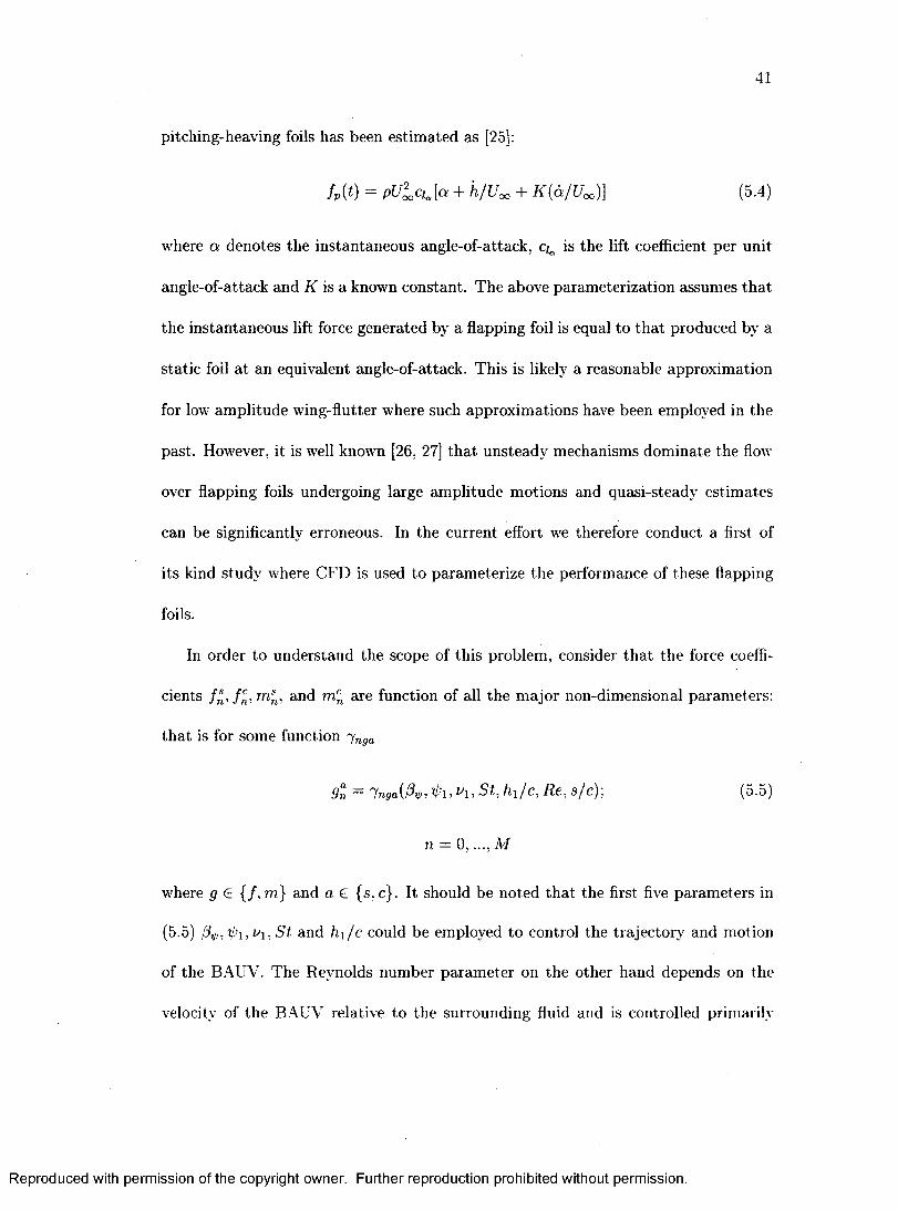
pitching-heaving foils has been estimated as [25]:

fp{t) = pUl^ci^[a -f h/Uoo + K (q/Voc)] (5.4)

where a denotes the instantaneous angle-of-attack, is the lift coefficient per unit

angle-of-attack and K is a known constant. The above parameterization assumes that

the instantaneous lift force generated by a flapping foil is equal to that produced by a

static foil at an equivalent angle-of-attack. This is likely a reasonable approximation

for low amplitude wing-flutter where such approximations have been employed in the

past. However, it is well known [26, 27] that unsteady mechanisms dominate the flow

over flapping foils undergoing large amplitude motions and quasi-steady estimates

can be significantly erroneous. In the current effort we therefore conduct a first of

its kind study where CFD is used to parameterize the performance of these flapping

foils.

In order to understand the scope of this problem, consider that the force coeffi

cients and are function of all the major non-dimensional parameters:

that is for some function 'Ynga

9n = V’l , 2 1 , St, Re, s/c); (5.5)

n = 0,..., M

where 5 G { /, m} and a G {s. c}. It should be noted that the first five parameters in

(5.5) /3 ,, L’l, J/i, 5 / and /ii/c could be employed to control the trajectory and motion

of the BAUV. The Reynolds number parameter on the other hand depends on the

velocity of the BAUV relative to the surrounding fluid and is controlled primarily


42

by the main propulsor. Finally, the last parameter s /c is a design parameter and

is assumed fixed for a given pectoral fin. Thus a complete parameterization of the

performance of the flapping foil for the BAUV conceptual model requires tha t the

CFD simulations extract the dependence of the force coefficients on the first four

parameters as well as the Reynolds number.

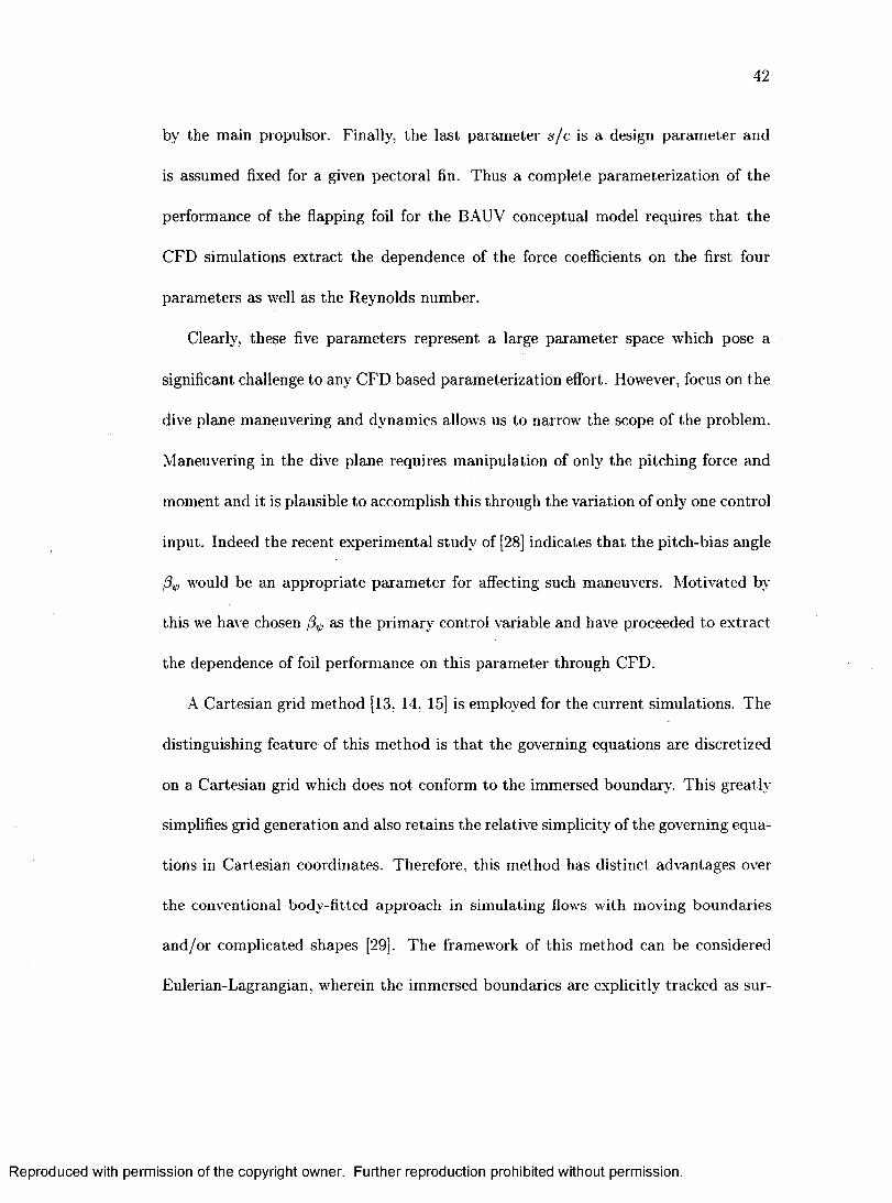
Clearly, these five parameters represent a large parameter space which pose a

significant challenge to any CFD based parameterization effort. However, focus on the

dive plane maneuvering and dynamics allows us to narrow the scope of the problem.

Maneuvering in the dive plane requires manipulation of only the pitching force and

moment and it is plausible to accomplish this through the variation of only one control

input. Indeed the recent experimental study of [28] indicates that the pitch-bias angle

would be an appropriate parameter for affecting such maneuvers. Motivated by

this we have chosen as the primary control variable and have proceeded to extract

the dependence of foil performance on this parameter through CFD.

A Cartesian grid method [13, 14, 15] is employed for the current simulations. The

distinguishing feature of this method is that the governing equations are discretized

on a Cartesian grid which does not conform to the immersed boundary. This greatly

simplifies grid generation and also retains the relat ive simplicity of the governing equa

tions in Cartesian coordinates. Therefore, this method has distinct advantages over

the conventional body-fitted approach in simulating flows with moving boundaries

and/or complicated shapes [29]. The framework of this method can be considered

Eulerian-Lagrangian, wherein the immersed boundaries are explicitly tracked as sur-


43

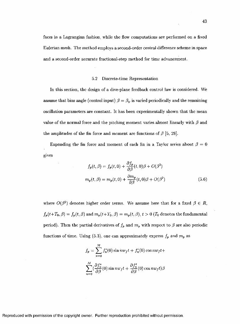
faces in a Lagrangian fashion, while the flow computations are performed on a fixed

Eulerian mesh. The method employs a second-order central difference scheme in space

and a second-order accurate fractional-step method for time advancement.

5.2 Discrete-time Representation

In this section, the design of a dive-plane feedback control law is considered. We

assume that bias angle (control input) /? = is varied periodically and the remaining

oscillation parameters are constant. It has been experimentally shown that the mean

value of the normal force and the pitching moment varies almost linearly with and

the amplitudes of the fin force and moment are functions of (3 [5, 28].

Expanding the fin force and moment of each fin in a Taylor series about = 0

gives

'?) — fp{t, 0) +

rupit, 13) = mp{t, 0) 4- ^ ^ ( t , 0)/3 + 0(/3^) (5.6)

where O{0^) denotes higher order terms. We assume here th a t for a fixed (3 E R,

fp{t+To, (3) = /p(t, P) and mp{t+TQ, P) — mp{t, 3), t > 0 {Tq denotes the fundamental

period). Then the partial derivatives of fp and nip with respect to 3 are also periodic

functions of time. Using (5.3), one can approximately express fp and nip as

Mfp = Y l /"(O) sin nwft + /^(O) cos nwft-\-

n = 0

M

X ^ ( ^ ( 0 ) sin nwjt 4- ^ ( 0 ) cos nwft )p


Mrrip = y~^ (0) sin nWft + m% (0) cos nwjt-\-

n = 0

M

sinnw /f + ^ ^ ( 0 ) cosnwjt)Pn= 0

where 0{pP) terms are ignored in the series expansion. We define

44

(5.7)

/ . = (Æ(0), s m , / f (0). , &(0), & (0)F

A = ( f ( 0) . f ( 0 ) , f ( 0) , ^ ( 0) , ^ ( 0 ) f

m„ = (m S(0),m ;(0),m ;(0),....,m ;„(0),m 5,(0))’'

am i, dm%a # a a

f a - , f b , ' m a , m b all G Using (5.7) and (5.8), we get

(5.fO

f p { t ) = ( f { f a + P f b )

<t>

mp{t) = (p^irria 4- Prrib)

1 sinwft ..... s inM w f t cosMwjt

(5.9)

The vehicle has two attached fins; therefore the net force and moment are fp^ —

—2fp and rupy = 2{dcgjfp + rUp), where dcgf is the moment arm due to the fin location

(positive forward). The dive plane dynamics (2.3)

X = Ax + Dfp

rur.

can be written as

(5.10)


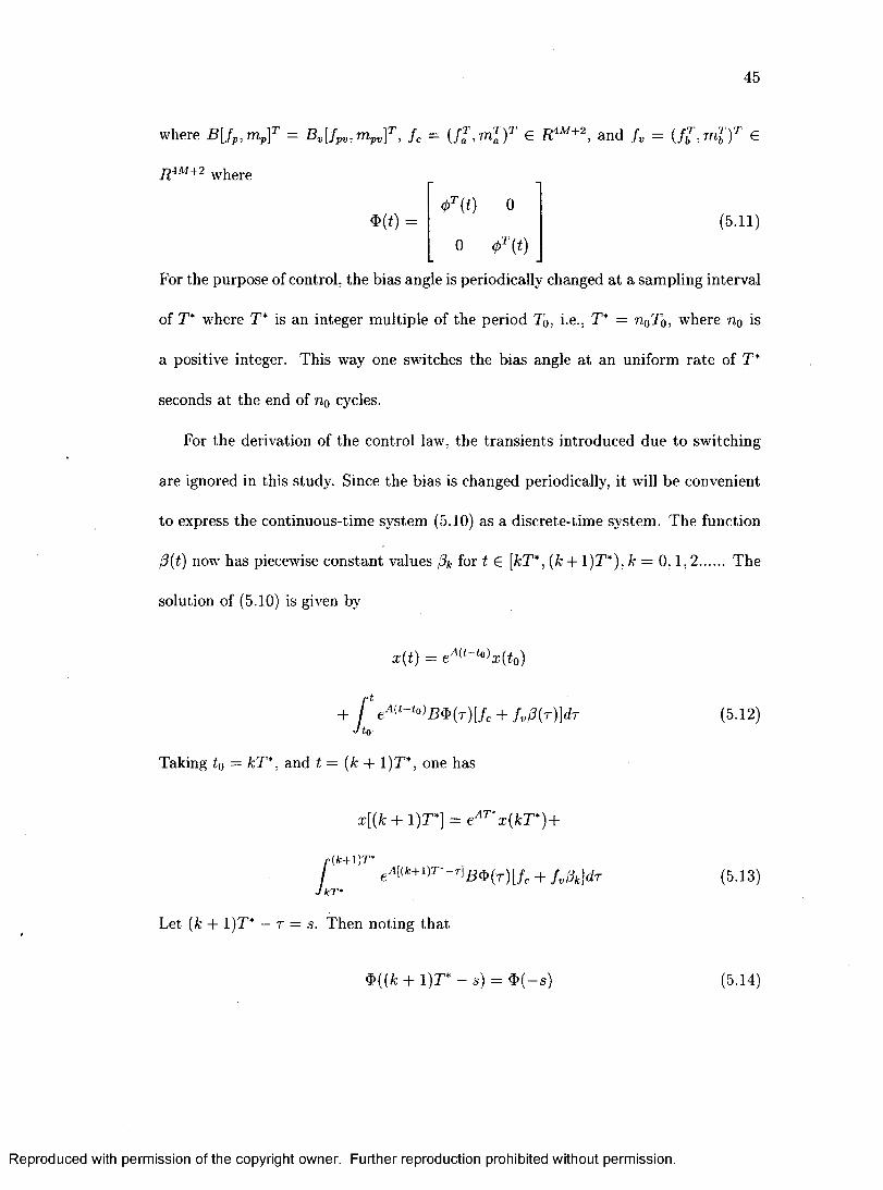
(5.11)

45

where B [ fp ,m p f = By[fpy,mpyf, A = 6 and R = (/^', mg )^ G

J iA1 + 2

4> {t) 0

0

For the purpose of control, the bias angle is periodically changed at a sampling interval

of T* where T* is an integer multiple of the period To, i.e., T* = noTo, where no is

a positive integer. This way one switches the bias angle at an uniform rate of T*

seconds at the end of no cycles.

For the derivation of the control law, the transients introduced due to switching

are ignored in this study. Since the bias is changed periodically, it will be convenient

to express the continuous-time system (5.10) as a discrete-time system. The function

P{t) now has piecewise constant values pk for t G [kT*, {k+ 1)T*), k = 0 ,1 ,2 ...... The

solution of (5.10) is given by

x{t) = e' *‘“‘® a:(io)

-F r 4- A/3(T)]dT (5.12)Jto

Taking to — kT*. and t = {k + l)T*, one has

x[{k 4- 1)T*] = x{kT*)+

-{k+OT*/ (5.13)

JkT'

Let [k 4- 1)T* — T — s. Then noting that

4>((fc -h l ) r - s) = $ ( - g ) (5.14)


46

(5.12) gives

x[{k + 1)T*] = x{kT*)+

r e ^ 'B $ (-s ) [A + A W aJo

= Adx{kT*) + BdPk + d (5.15)

where Ad = and B q = s)ds, Bd — BoR E R^, and d — BoR € 7? .

The output variable (z) is

0 0 1 0 z ( tT ') = Cdi(kT') (5.16)

The transfer function relating the output y{kT*) and the input Pk (assuming that

(7 = 0) is given by

M = G(z) = Q (z7 - yld)-^Bd =;9(z)

^ + fh){z + //2)(z + P's)^ Z' + UgZ + 0-2Z + OiZ + Wo

where z denotes the Z-transform variable, /x,(z = 1,2,3) are real or complex

numbers and kp and api = 0 ,1 ,2 ,3) are real numbers.

It is assumed that the pectoral fins are attached between the eg and the nose

of the vehicle. For the AUV model under consideration, the number of unstable

zeros (i.e. the zeros outside the unit disk in the complex plane) depend on the

distance {dcgf) of the pectoral fins from the eg. It has been found that there exists a

single unstable zero if the fins are attached closer to the eg, but two unstable zeros

appear if the attachment distance dcgf exceeds a critical value. Thus the transfer

function G(z) has at least one unstable zero, and it is nonminimum phase. Of course.


47

the continuous-time AUV model has only two zeros but the pulse transfer function

G{z) has three zeros. For this nonminimum phase AUV model, it is not possible to

synthesize an inverse controller. Here we modify the controlled output variable so

that the new transfer function is minimum phase and then derive the inverse control

law for approximate depth trajectory control.

5.3 Minimum Phase System

In this section, the derivation of a minimum phase approximate model for a nth

order single-input and single-output nonminimum phase system is considered. For

this purpose, the original transfer function is simplified by ignoring its unstable zeros.

We consider a single-input single-output (SISO) of the form (5.15) and (5.16) with

<7 = 0 (denoted as {Ad, Bj-Cd)) where x G 77", Ad G 77"^", and suppose tha t the

system has Qs stable and unstable zeros. The transfer function relating the output

y{kT*) and the input pk of the system {Ad, Bd, Cd) (assuming th a t <7 = 0) is

M = G(z) = Q (z7 - ^ (5.18)P{z)

where the nth order characteristic polynomial A(z) is

A(z) = det{zl — Ad\ = z" -T ' -t-..... -+■ tijZ -h oo (5.19)

and the numerator polynomial is

Qv Qsrid{z) = kp J J ( z + iiyj) Y%(z -t- Psj) (5.20)

j=i j=i

where a, (7 = 0,1,..., n —1) and kp are constants, y u j { j = 1, and fj,gj{j = 1,..., g.,)

are unstable and stable zeros of the transfer function, that is \fj,uj\ > 1 and |psj| < 1-


48

For obtaining a minimum phase approximate system, one removes the unstable

zeros of G{z) but retains the zero frequency (dc) gain. Thus the approximate transfer

function Ga{z) takes the form

Qv Çs

Ga{z) — kpA. (z) J ^ ( l + T Hsj) =j=i 7=1

{hqszA + .....+ fiiz + /io)A“ ^(z) (5.21)

The approximate transfer function Ga{z) has now qs stable zeros but the poles of

G„(z) and G(z) coincide.

We are interested in deriving a new controlled output variable ya such that

T / . ( t r ) = C.z(A;T') (5.22)

and

^ = G .(z) = C.(z7» - Ad)-'Bd (5.23)

where C„ is a new output matrix which is yet to be determined. Using the expression

of the resolvent matrix (inverse of (z7„ — A^,)), one can write Go(z) as [30]

Ga(z ) = A ^(z)[(z" ^ + a n _ i z " ^ + .... + Oi)C'oBd+

(z" + a„_iz" ' + ....a2)Ca-4(/Brf + ............+ (z + a„-i)GaA^

+C .A 3-'B^] (5.24)

The relative degree r of Go(z) is r — n — q ,, and therefore one must have

C.,4;B^ = 0 ,; = 0 , l , . . . . , r - 2

(5.25)


49

Using (5.25) in (5.24) gives

+Or)Ca^d Bd + ...... +

[z + a„_i)CûA^ Bd + CaA'^ Bd] (5.26)

Noting that Qs = n - r , using (5.25) and equating the numerator polynomials of (5.21)

and (5.26) gives

CaA^dBd + ^Bd —

+ .... + Or-t-lCaAj Bd — hi

+OrCa,4^ ^Bd — ho

Collecting (5.25) and (5.28). one obtains the matrix equation

CaL = hf

where

(5.27)

(5.28)

and the n x n matrix L is obtained0 0 . . . 0 h g s h g ^ ^ i . . h i h o

by comparing a matrix equation with (5.28). Assuming that the system (5.15) is

controllable, one has that rank [Bd,AdBd, ,A'^~^Bd] — n [31-33]. In view of

(5.28), it follows that the columns of L are independent. Then solving (5.28) gives

(5.29)


50

To this end, a question arises: How close is the new output ya{kT*) to y{kT*)7 In

view of (5.18) and (5.21), it is seen that the modified output ya{kT*) and the actual

depth y{kT*) are related as

qvy{z) = Y%(zT Huj)A + IInj)~^Mz) = Gf{z)ÿa{z) (5.30)

7=1

According to (5.31), the actual output is obtained by passing ya{z) through a filter

which has the frequency response (amplitude and phase response) given by

Gf{e^'*'^ ) = jQ (e ''^ + A*a«7)(1 + (5.31)7=1

Apparently if the zero locations and the frequency uT* are such that

+ t i u j ) « 1 + l ^ n j , j = 1, - , q u (5.32)

then it follows that

C/(e'"'^') « 1 (5.33)

That is the gain of Gf{z) is 1 and

!/(7rT') % i/ .(A r ) (5.34)

When ya{kT*) asymptotically converges to a constant value y* one can take tc = 0

and in this case, the actual output y converges to y*. Thus it follows that if (5.34) is

valid, then the synthesis of the inverse controller designed for the trajectory control

of the modified output y„ accomplishes accurate control of the depth trajectory. In

the next section, an inverse control law is designed for the tracking control of the

modified output y„-


51

5.4 Inverse Control Law

Consider now a new system

4 l ) r ] = 4 + d

) (5.35)

where x E 77", ya{kT*) and pk are scalars and the output y ^ k T * ) is the modified value

of y[kT*) . Suppose a reference trajectory y R k T * ) is given which is to be tracked by

ya{kT*). In view of (5.35), using it recursively one has that

4 l ) r ] = C .4 j z ( & r ) 4 C .d (5.36)

!/.[(t 4 2)T*] = C ..4 ^ i(tT ') 4 C .A jd 4 C .d

r - 2

y .[ ( t 4 r - l ) r ] = C .,4 ; - :z (7 r r ) 4 T? = 0

r - 1

!/.[ (t 4 r ) r ] = C . , 4 ; z ( t r ) 4 4 (5.37)ï=0

The system has relative degree r. Therefore, the input pk appears for the first time

in y„[{k 4 i)T*] for i = r.

We are interested in tracking the reference trajectory yRkT*). For this purpose,

we choose the control input pk as

r—1= (C .A ;-:B d )-'[-Q .4 ^ z (k T * ) - ^ C . A X 4 %] (5.38)

1 = 0

where the signal Vk is selected as

r—]t'k = ?/r[(A- 4 r)T*] - ^ p , ( C » 4 : r ( A r )

1=0


52

i-l+ ^ C .A y - ! /r [ (A : + 7 )r ]) (5.39)

7=0

where pi {i = 0,1, ....r — 1) are real numbers. Defining the tracking error e{kT*) —

VaikT*) — yr{kT*), and using the control law (5.39) and (5.40) in (5.38) gives

e[{k + r )T * ]+ P r-A {k + r - l ) T * ] + ....

-\-pie[{k + l)r* ] 4 poe{kT*) = 0 (5.40)

The tracking error satisfies a rth order difference equation. The characteristic

polynomial associated with (5.41) is

(z^ 4 Pr-\Z^ 4 .... 4 Po) = 0 (5.41)

The parameters pi are chosen such that the roots of (5.41) are strictly within the

unit disk. Then it follows that for any initial condition x{0),e(kT*) 0 as k —4 oo

and the controlled output y„(A:T*) asymptotically converges to the reference sequence

yr{kT*). Furthermore, as described in the previous section, according to (5.34) for

slowly varying y^kT*) , y{kT*) follows yRkT*) accurately.

5.5 Simulation Results

CFD Param eterization

In the current simulations we employ a two-dimensional {s/c — oo) 12% thick

foil with an elliptic cross-section. The Reynolds number is fixed at a relatively low

value of 300 which alleviated the grid requirements for the simulation. In addition,

fii/c, '01 , Ui and Si are fixed at value equal to 0.35, 30". 90" and 0.4 respectively. A


53

non-uniform 161 x 111 Cartesian mesh is employed in the simulations where the grid

is clustered in the region around the flapping foil and in the foil wake.

Figure 5.1 shows the computed flow for the = 0" and 20" cases at the time

instant when the foil is at the center of its heave motion. The plots show contours

of spanwise vorticity (which is the curl of the velocity field) as well as the velocity

vectors. For the = 0" it is observed that the flapping foil produces a vortex street

in the w ake w^hich is comprised of counter-rotating vortices. The occurrence of such

vortex streets is quite well knowm [34] for these flows. The vortex street is along the

direction of the flow and produces a jet-like flow in the streamwise direction. For the

Pg, = 20° flow, the vortex street it oriented at an angle to the freestream and results

in a vectored jet.

Figure 5.2 show s the time variation of the resultant pitching force {fp) and mo

ment {nip) on the foils for these two cases. These quantities are presented as non-

dimensional coefficients wherein the force and moment are non-dimensionalized by

QocC and QocC with q c = ^pU^- The plots clearly show that both the force and

moment are periodic in time with the magnitude of variation in the pitching force

being much larger than tha t of the moment. This force and moment coefficients

can then be decomposed into their Fourier decomposition. Table 1 and 2 show the

nondimensionalized force and moment coefficients for the bias of zero and 20 degrees,

respectively.

Table 1. Table showing various components of force and moment coefficient for

the Pg, — 0" case.


54

n

0 0.00 0.00 0.00 0.00

1 -1.89 -1.56 0.52 0.35

2 0.03 -0.04 0.00 0.01

3 -0.93 -0.08 -0.06 0.00

4 0.00 0.00 0.00 0.01

Table 2. Table showing various components of force and moment coefficient for

the = 20° case.

n m» K

0 2.97 0.0 -0.47 0.0

1 -2.93 -2.00 0.69 0.07

2 -0.81 1.58 -0:02 -0.13

3 -0.84 -0.21 -0.07 -0.04

4 0.09 0.22 0.02 0.02

In addition to these two cases, two other cases wdth Py, = 10° and 30° have been

simulated (data not showm here) and these data are used in the simulation of the

BAUV dynamics as described in the subsequent subsection.

D ive-plane Trajectory Control

In this section, simulation results using MATLAB and SIMULINK are presented.


55

The parameters of the model are taken from [7]. The key vehicle parameters are

I = 1.282 (m), mass=4.1548 (kg), Iy= 0.5732 (kgm^), xg = 0, zg — 0.578802e — 8;

and the hydrodynamic parameters are taken as z' = —0.825e — 5, = —0.825e — 5,

z'g = -0.238e - 2, = -0.738e - 2, = -0.16e - 3, = -0.825e - 5, M'g =

—0.117e — 2, and A/^ = 0.314e — 2. The uniform forw^ard velocity of the vehicle is 0.7

(m/s). Four cases (S l,E l) and (E2,S2) of pectoral fin attachments are considered. In

the first tw o cases (S i,E l), fins are attached at the eg (i.e., the moment arm Rgf — 0)

and in the other case they are located at a distance of dcgj = 0.15 (m) ahead the eg.

The fins are assumed to undergo heaving and pitching motion and the frequency of

oscillation is taken to be 4 (Hz) {u)f = 25.1327(rad/s)). Thus the period of oscillation

is To = 0.25 (sec), but the sampling period is taken as T * — 0.5 (sec) (twdce the

period of oscillation). The initial condition chosen is x(0) = 0.

Smooth reference trajectories are generated by a command generator of the form

{ E ^ + Pc2-F^ + PclE + P c J o ) y r { k T * )

— (1 3 - PcO + P c i A P c 2 ) y * ( k T * )

for cases (S1,E1) and for (S2,E2) the command generator is

(T" + PcsE^ + PciE^ + PciE + Pco)yr{kT*) =

(1 + PcO + P e l + Pc2 + P c 3 ) y * ( k T * )

where E denotes the advance operator [ E y R k T * ) — y r [ { k + 1)T*]) and the param

eters Pci are chosen to be zero so tha t the poles of the command generator are at


56

z = 0. These two reference trajectory generators are simulated using their state

variable forms with states = {xr\,Xr2 ,Xr3 y and = (Xri,Xr2 ,Xr3 ,Xr4 y \ respec

tively. For generating exponential and sinusoidal reference trajectories, the command

inputs chosen are Y*{kT*) = d*{l — exp{—akT*)) and Y*{kT*) = d* siii{uJrkT*)

where a = 0.2, = 0.2 (rad/s), and d* = 1 (m) is the target depth or the am

plitude of the sinusoidal depth trajectory. The initial condition of the command

generator is Xr(0) = 0. The Fourier series representations of the fin force and mo

ment obtained using CFD have four dominant harmonics; and therefore one has

(p(t) = [l,sm{wft),cos{wft), .. ,sm{4wft) ,cos{4wft)^. Of course the design approach

does not limit the number of harmonics for control law derivation. The Fourier coef

ficients in (5.7) and (5.8) derived using CFD are used for simulation.

The zeros of the pulse transfer function depend on the fin attachment distance

dcg/E [0, 0.2] (m). The transfer function G{z) for case (SI) has zeros at 0.8695, 1.5464

and 0.3299; but for (82), the zeros are -1.0206, 0.2343 and 1.2731.

The new- output pa in (5.22) is computed using the solution of (5.29). For the

AUV model, the relative degree r of the modified output for (S1,E1) is two, but for

(82,E2) is 3; and therefore the control law- (5.39) depends on the fin location and they

are not identical for cases (81,E l) and (82,E2). For case (81,E l), the tracking error

equation takes the form

{E' ^ PiE-i-po)e{kT*) = 0

but for for case (82,E2) one has third order error dynamics

(B= -h 4- piE 4- Po)e(AT') = 0


57

where for simulation it is assumed that for (S i,E l) po = 0.01 and pi = 0.2; but for

(82,E2) Po = 0.001, Pi = 0.03 and p2 = 0.3. This gives the poles of the error dynamics

at z = —0.1 for each case which are well within the unit disk in the complex plane.

Case 1. Sinusoidal Trajectory Control Case (SI): Fin oscillation period

To = 0.25 (s), sampling period T* =0.5 (s), Rgf = 0.15(m)

Sinusoidal reference trajectory is generated by setting Y*{kT*) = d* sin(0.2A:T*)

as the depth command input with d* = 1 (m). The responses are shown in Fig. 5.4.

We observe that the response of the modified output {ya{kT*)) converges quickly to

the command trajectory yPkT*). The actual depth, modified depth and reference

trajectories remain very close. The intersample values of the depth response has

oscillations of minor amplitudes, but it tracks the command trajectory.The maximum

pitch angle and pitch rate are less than 20 (deg) and 50 (deg/s), respectively and the

maximum value of w does not exceed 0.75 (m/s). The maximum bias angle is about

1.2 (deg). The control force is about 30 (N) and the control moment is less th a t 0.4

(Nm).

Case 2. Sinusoidal Trajectory Control Case (S2): Fin oscillation period

To = 0.25 (s), sampling period T*=0.5 (s), d^gj = 0

8imulation is done for tracking sinusoidal trajectory similar to case 2, here one

has dcgf=0 (m). Fig. 5.5 shows the selected responses. We observe that the controller

accomplishes accurate trajectory control. The depth response is smoother,the bias

angle is larger. Furthermore, the bias angle undergoes more switchings.

Case 3. Exponential Trajectory Control Case (E l): Fin oscillation period


58

To = 0.25 (s), sampling period T* =0.5 (s), dcgf = 0.15(m)

To examine the effect of the attachment point of the fins, it is assumed that

dcgf — 0.15 (m) (i.e, fin is located ahead the eg). The remaining parameters of case 1

are assumed. The plots are shown in Fig. 5.6. It seems that placing fins away from

the eg provides better performance. This is attributed to the extra pitching moment

provided by the normal force when the moment arm is nonzero. We state this after

comparing this case with the case where dcgf = 0 (m).

Case 4. Exponential Trajectory Control Case (E2): Fin oscillation period

To = 0.25 (s), sampling period T* =0.5 (s), dcgf — 0(m)

To examine the effect of the attachment point of the fins, it is assumed that

dcgf = 0 (m). The remaining parameters of case 1 are assumed. The plots are shown

in Fig. 5.7. The response is smoother but the other performances are not as good as

that of the earlier case.


59

Figure 5.1: Spanwise vorticity contours and velocity vectors for flow past the flapping foil ay two different bias angles of 0° and 20°. Note that velocity vectors are shown on every fourth grid point in either direction.


60

1I1 i

1.75 3.5 time 5.25

(b)m p

s15

1.75 3.5 5.25time

Figure 5.2: Fin force and moment for /? = 0 and 20 (deg)


61

Zeros vs Deg2.5

gI

{Ia

0.5

Î0

N- 0.5

- 1.50 0.04 0.06 0.08 0.1 0.12 0.16 0.18 0.2

Deg

Figure 5.3: Zeros of the pulse transfer function


62

fa.if

0.4[

*{ -0.4

10 20 S3Trtnes)

1C- 20Tm#aq

lYiliiiiiimmffiiAeisKi


63

I \

I III

5

Figure 5.4: Sinusoidal Trajectory Control Case (Si)

I.

1 1

0 10 K - 30 0 10 « 30


64

10 2 e 30Tirneisec) imersec

fe 0.I5 - 5 .

Œi

.lS->

-20.

-25,

P:kr A?^.iccgi

Figure 5.5: Sinusoidal Trajectory Control Case (82)


65

?

0.5£

%tj

- 0.50 10 20 30

«!0.

-10

-150 10 30

Timejsec! Tme(seC)

Time seci10 20

Timeisec)

Tmwseci0 10 20

Titnejsec)

- 0.410 20

Time(sec)30


66

50 s,

£ Os

Ai AW \

\ I-50 X 15

\

0

Piich Angle,(degj

-10

-15 0

3025

2015

Timejsec)

Figure 5.6: Exponential Trajectory Control (E l)

5.2;

Î

0 !

10 3GTirselsesi 10 2C 3DT:m6<SK=


67

I - 5 0

0 10 2D 10 % 30Tiit»(S€C)

ID 20 30Tmiseci

I 10^ -15

Righ

Figure 5.7: Exponential Trajectory Control (E2)


CHAPTER 6

CONTROL OF OSCILLATING FOIL FOR PROPULSION

The contribution of this chapter lies in the design of a control system for the indepen

dent asymptotic control of the lateral and rotational motion of a 2-D hydrofoil based

on the internal model principle (servomechanism theory). The foil is spring driven by

two actuating signals and it experiences lateral displacement and the angular rotation

in the free stream. The foil model includes hydrodynamic forces computed using the

theory of unsteady aerodynamics. A command generator is used to generate specified

command trajectories which are linear combinations of sinusoidal functions of distinct

frequencies, amplitudes, phase angles and average values. A feedback control law is

designed so that plunge displacement and pitch angle of the foil asymptotically tracks

the command trajectories generated by the command generator. The control system

includes a servocompensator which is fed by the lateral and rotational trajectory er

rors. Since the states associated with the Theodorsen function cannot be measured,

an observer is designed to obtain the estimates of the unavailable states. Then the

controller is synthesized using the estimated state variables. Simulation results are

presented which show that in the closed-loop system, independent asymptotic control

of the plunge displacement and pitch angle trajectories are accomplished.

68


69

6.1 Mathematical Model

The spring driven hydrofoil including a lateral spring is shown in Fig 6.1.

L and M are the hydrodynamic lift and moment and Fa and Ta are the driving

force and torque applied to the foil at the axis of rotation by the lateral rotational

springs controlled by two independent actuators. (The rotational spring is not shown

in figure). The complete equations of motion of the foil based on the unsteady aero

dynamic theory has been derived in [18] which are given by

m {zt + 9tb) = L + Fa (6.1)

JOt — M + Ta — Fab (6.2)

where Zt is the vertical position (plunge displacement) and 6t is the angular posi

tion (pitch angle) of the foil, m is the mass, J is the moment of inertia, and b is

the position of the axis of rotation along the chord. A complete derivation of the

hydrodynamic lift and moment including the added mass and wake effect based on

unsteady aerodynamic theory has been obtained in [18]. The lift and moment are

given by

T = 7T/)[2o[/(-Z( 4- 4- (^ - 6)0()C(iw)-F

a^(—Zt Uêf — bOf) (6.3)

M — —2tvp o U {— )9t T pc?U {—Zt 4 -1/(—zt 4- U 9tF

—b)9t)C{iio) — —pa^9t (6.4)

where p is the density, a is the half chord length of the tail, U is free stream ve

locity (or equivalently fish’s forward motion), and C(ia;) is the theodorsen function.


70

A third-order transfer function to obtain a good approximation of the Theodorsen

function used in the study is

C(iw) = + 02 (*<7 ) + aij icr) + ap {ia)^ -t- 6 2 (1(7 ) -I- fei (a) + bo

where a — ^ is the non-dimensional reduced frequency and a, and bi are given by

[0 3 , og, o i, Oo] = [0.500000,1.07610,0.524855,

0.045133]

[62 61 60] = [1-90221,0.699129,0.0455035]

The force and moment. Fa and Ta applied to the foil by springs in series with the

actuators are

F a — F ^ i ^ Z a Z f ^

Ta = Ke{9a — 9t) (6.5)

where Kz and Kt are spring constants, and and 9a are the positions of the lateral

and rotational actuators. According to biomechanists, fish have compliances in their

tail tendons to reduce energy costs of muscles. Harper et al have demonstrated in

[18] that these springs can similarly reduce actuator energy.

Oscillating foil produces periodic forces and moments which can be utilized for

the propulsion and control of AU Vs.

Suppose that

Zr(f)

^r(f)


71

is the specified reference trajectory. These trajectories are generated by exosystems

given by

n,(g)zr(g) = 0

nfl(s)0 r(s) = 0

where Zr and Or denote Laplace transforms of Zr{t) and Orit), respectively, and L[z(s)

and rig(s) are appropriate polynomials of the form

In these polynomials, and are distinct positive real numbers. We are interested

in deriving a control law Uc = {zg, Og)^ such tha t in the closed loop system the output

vector Y = {zt,9tŸ asymptotically follows the reference trajectory Yr{i), tha t is, the

tracking error Ÿ = [(z — z,), {9r — 0t)]^ converges to zero as t —> oo . Note that by

the choice of the initial conditions , where i — 0 , 1 , 2 , 3....{mz — 1 ), where

j — 0 , 1 , 2 ....{me — 1 ) and frequencies wgj, one can generate a linear combination

of of sinusoidal trajectories of desirable amplitude, phases, biases and frequencies, in

order to produce required control force and moment for the control of AUV. Presently,

there is considerable interest in exploring the relationships among the fin forces and

moments and the modes of oscillation (feathering, lead-lag, and flapping motion) and

oscillation parameters of the foils , and numerical and experimental results have been

obtained.


72

6.2 State Variable Representation

For the purpose of control system design, it will be convenient to obtain a state

variable representation of the hydrofoil and the reference trajectory generator.

The Theodorsen function can be treated as a filter with input

V / — —Zt + U 9t — b)9t — C f k

and output

= C(a)T}(s)

where C{s) is obtained by substituting io by ^ in C{iuj)

The transfer function C(s) can be written as

4- fi-iS + /lo

Zt4- Cfd

9t 9t

(6 .6)

(6.7)

C’(s) — fic 4- (6 .8)4- P 2 S + P i S 4- po

where fig =aa and hi and p, are appropriate real numbers. Although it is possible to

obtain infinitely many realizations of C(s), one can obtain a minimal realization of

dimension 3 in the form

0 1 0 0

0 0 1 Xf 4~ 0

—Po -Pi - P 2 1

Vf

1/1

/ \Zt

\ 0 , J

+ A/2 4- A f 3 X f (6.9)

— hcVf 4- h()Xfi 4- h\Xf 2 4- h2 Xj3


73

= hrCc'- fk

f \ ( \Zi Zl

+ Cfd^ 9t J

+ Cf^Xf (6 . 10)

whereT

2I /1 = ^ 0 0 I j Cfk

41/2 = f 0 0 Cfd

Cf2 — ho hi li2 ^Collecting the coefficients of of f* and 6 t, one obtains from (6.1) and (6.2)

M

where Uc

( \ ( \ / \i'l Zt Zi

= D + /i

/ ' !\ T

+ KfY f + B qUc

is the control input,

m + Trpa mb + Tipa^bM

D —0 ■npa^U

0 —27rp^f/

- K z 0 2tt paUK = ^ K f =

bl<z —he TTpa^U

Bo0

-bKz Ke

(6 .11)


74

Substituting for Yj from (6.10) and solving for I g) j gives

( \ / \Zi

+ M -R D +

kfhcCfd)

y y

\ 0 t J

+ Ay C /2%/ +

= Ai

( \Zt

\+ Ao

( . \Zi

\ 6 i J

+ A 3 X f + B\Uc

Define the state vector

= Zt Bt Zt 6t %/ j J

A state variable representation of (6.9) and (6 .1 2 ) takes the form

X =

0'2x2 h x 2 0 2 x 3 02 X1

Ai A 2 A3 X + Bi

"4/1 A f 2 A/3 03*2

Ur

= Ax + BUc

(6 .12)

(6.13)

(6.14)

where the system matrices are A f and B f The output vector Y is then

written as

] ' = C r ^2x2 02x5 (6.15)


75

6.3 Control Law

In this section, the state variable model (5.14) is used for the derivation of a

control law such that y{t) asymptotically tracks yr{t).

Suppose that the polynomial equation

n x 0 )n@(s) = 0

has (2m 4- 1) distinct roots 0 and ijw,-, i = 1,...., m.

Define a polynomial n^(s) as

Ile(s) = s{s^ 4- Wi^) (s^ 4- Wjn )

(6.16)

— 4- «0.2771-1 4- 4- «C.36' 4-«ciS (6.17)

/ - \nr'(a) 0 4(g) - 4(g)

0 nrXs) 9r{s) — f(g)

Note that llf,(s) is an odd polynomial.

For the derivation of control law, consider servocompensators driven by the error

signals {zr — z,) and {9r — 9i) in the form

f) zLt.sl — At.sl(6.18)

A state variable representation of the transfer matrix (llg(s), 11 can be easily shown

to be

X s z — A g Z g ; 4" B g { Z r C'l%)

1 cz — ^ 1 0 ] x 2 m ^ ~

x's0 = AgXse + Bs{9r - C2 .t)

Yc0 = CsXsff (6.19)


76

where

0 1 0 0 0

A s - 0 0 1 0 , B s = 0

0 — «cl 0 . . . — O c 2 m -l 1

Define the augmented state vector

z . = R ~

Then the derivative of Xa can be written as

+ 2 (2 m + l)

A 0 0 B

Xg — - c - i A s 0 Xg + 0

— C‘2 0 A . 0

t/c +

0 0

z,.Bs o

Or0 B,

A g X a + B qU c + B d { Z r . Or) (6.20)

For the asymptotic trajectory tracking of Yr{t), according to the servomechanism

theory, one must find a control law of the form

Uc = -Ka'Xa (6.21)

such that the closed-loop matrix

Aflc — (A„ — B „ K a ) (6 .22)


77

is Hurwitz (i.e, all its eigenvalues have negative real parts.) For the computation of

this, one can use optimal control theory or pole assignment technique. In this study

Ka has been obtained assigning eigen values of Age in a stable region of the complex

plane.

6.4 Observer Design

For the synthesis of control law (6.21), the measurement of the state vector x is

essential. However, the state of the filter associated with the Theodorsen function

cannot be measured. As such it becomes necessary to obtain estimates of Xf.

For the state estimation, consider an observer given by

& = Az + BUc + F ( y - Cz) (6.23)

which gives the dynamics of state error x — x — x in the form

k = { A - FC )x = Aoi (6.24)

For the convergence of the state estimation to zero, one selects F such that the

eigen values of A q are on the left half of the complex plane. Again, one can use the

optimal control theory or the pole assignment technique for the computation of F .

In this study, we have used pole placement design approach for the computation of

the feedback matrix F .

For the synthesis of control law, the estimated states are substituted in (6.21) to yield

Uc = -K„[x^, (6.25)


78

In the closed-loop system, for any reference trajectory {zr-OrŸ which satisfies (5.16)

it follows from the servomechanism theory tha t {zt{t),6t{t)) tends to {zr{t),9r{t)) as

/ —> DO

6.5 Simulation Results

This section presents the results of digital simulation. The hydrodynamic pa

rameters are taken from [18] and are collected in the appendix. For an illustration,

reference trajectories of the form yr{t) = [A^ sin(w^t), Aesin{ujgt)Y' are selected where

Az = 0.04 (m) and Ag = 5 (deg). For the given yr, lle(s) = (s^4-u;^)(g^4-«/'g). and one

has XsztXgg E The augmented matrix A g has 7 stable and 8 imaginary eigenval

ues, and it is necessary to introduce feedback for the stabilization of the marginally

stable matrix A„. The feedback matrices Kg and F are determined using pole place

ment technique. These poles for simulation have been obtained by trial and error and

by observing simulated responses. For simulation, initial conditions are assumed to

be zero.

It is desired to control the foil so tha t the lateral displacement and pitch angle

trajectories oscillate with distinct frequencies, where = 4 and ujg = 6 (rad/s).

Simulated responses are shown in Figs. 6.1 and 6 .2 . It is seen that the output vector

{zi{t),6t{t)^ smoothly converges to the reference trajectory yr{t). After the initial

transient, which is of the order of one second, the lateral displacement and pitch

angle trajectories are sinusoidal functions of time and have specified magnitudes and

frequencies. The maximum tracking errors for the lateral and rotational motion are


79

5 (cm) and 6 (deg), respectively. The control inputs and have peak magni

tudes 5 (cm) and 2.5 (deg), respectively. The filter state vector associated with the

Theodorsen function are sinusoidal in the steady state. Simulation is also done for

uj\ = 6{rad/s) and wg = 4{rad/s) as well as for identical frequencies. Sinusoidal

trajectory tracking is smoothly accomplished in each case.


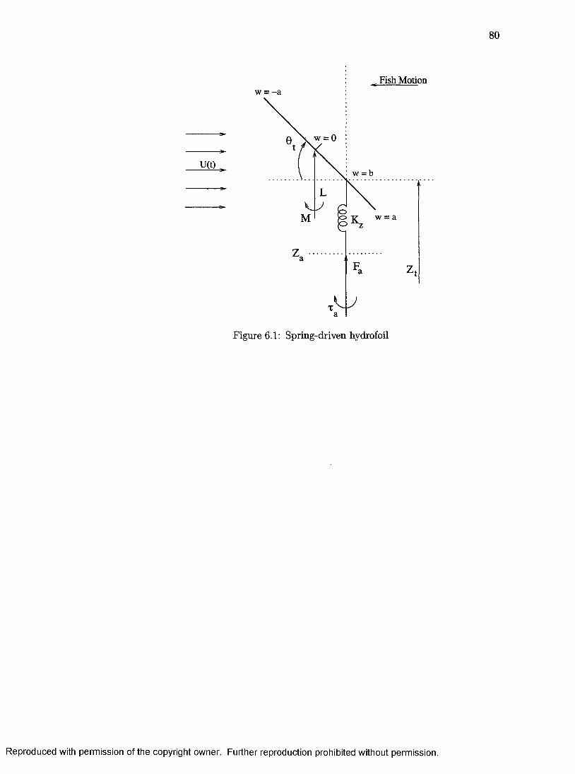
80

U(t)

Fish Motionw = -a

w = 0

w = b

oR K . w = a

Figure 6 .1 : Spring-driven hydrofoil


81

0.05

III

s-0.05

Thne(sec)

t 0

I

n

0.5 1 1.5 2Time(s8C)0.02

0.01

® - 0.01

1 -0.02

= 4 )0 3

-0.04

-0.050.5 1 1.5

Time (deg)

0.05

I

-0.05

Time{sec}

I

Time (sec)

0.05

In"

-0.05

-0.1

Time(s)

I

0.5Time


82

Time{sec)

- 0 5

- 1 5

0 0 5 1 15Tlme(sec)

0 5 1 1 5 2Time(8ec)

Figure 6.2: Oscillation Control: Case 1

-0.04

0 5 1 15Time(sec)

0 5 1 1.5Time(sec)

0.04

S 0.02

g -0.02

H -0.04

-0.06

Time(sec)

I

Time (deg)


83

0.051

I

4).D5'

Time(sec)

I

Time (» c)

0.15|

0.05

-0.05

-0.1

-0.15

-0.2

■ntne(s)

«

Time

>r-0 .5

0 .041

0.02

-0.02

-0.04J

Time(sec)

-20

Figure 6.3: Oscillation Control: Case 2


CHAPTER 7

CONCLUSION

The design of control systems for the dive plane maneuver using pectoral fins was

considered in the third and fourth chapters. Pectoral fins have lead-lag, feathering

and flapping modes of oscillations and have ability to produce maneuvering forces

and moments which are functions of oscillation parameters (frequency, amplitude,

bias angle and phase angle). The periodic forces and moments can be uniquely

characterized by the associated Fourier coefficients. An open-loop control law was

derived which determine a set of Fourier coefficients (i.e; fin forces and moment)

for finite time maneuver of the vehicle in the depth plane. Besides the open-loop

controller, a feedback control system was designed by utilizing periodically varying

bias angle of the fins as control input. The closed-loop controller was designed using a

discrete-time form of the model incorporating integral feedback. The complete open-

loop and closed-loop systems were simulated for various types of dive-plane maneuvers

which showed that using pectoral fins, one can perform precise and rapid maneuvers

using the open-loop and feedback controllers.

In the fifth chapter, biologically-inspired maneuvering of a biorobotic AUV using

pectoral-like fins was considered. The pitch-bias was updated at regular intervals

84


85

(multiple of the fundamental period). CFD and Fourier Series Expansion were used to

parameterize the effect of this control input on the hydrodynamical force and moment

produced by the flapping foil. For the purpose of design, a discrete-time model

was obtained and a nonminimum phase representation was derived for controller

design. Then an inverse control law for the trajectory control of the modified output

was derived. In the closed-loop system, the modified output and the actual depth

trajectory are sufficiently close to the desirable depth commands. Numerical results

for the exponential and sinusoidal reference trajectory tracking were obtained. From

these results, one concludes that accurate depth control along time-varying paths with

desirable pitch angle response can be accomplished using oscillating fins. Interestingly,

the control system gave better performance when the fins were attached away from

the eg toward the nose.

The sixth chapter has considered the control of oscillations of a 2-D hydrofoil

for the purpose of producing maneuvering and propulsive forces. Two springs for

transmitting forces to the foil have been used which are like the tail tendons of

fishes. Based on the servomechanism theory, a control law has been derived for the

asymptotic pitch and plunge oscillatory trajectory control. Simulation results showed

that in the closed-loop system the plunge and pitch can precisely follow sinusoidal

trajectories of distinct magnitudes and frequencies.


86

APPENDIX

SYSTEM PARAMETERS

The system parameters for simulation in chapters 2,3 and 4 have been taken from

[7]. The uniform forward velocity of the vehicle is 0.7 (m/s). The key vehicle param

eters are

/ = 1.282 (m) mass=4.1548 (kg) Iy= 0.5732 (kgm^)

ZG = 0 ZG = 0.578802e - 8

z( = -0 .8 2 5 e - 5 z: = -0 .8 2 5 e - 5

The hydrodynamic parameters are taken asz; = -0 .2 3 8 e - 2 z(, = -0 .7 3 8 e - 2

MÎ = -0.16e - 3 M4 = -0.825e - 5

M'g - -0.117e - 2 M ; = 0.314e - 2

The system parameters for simulation in chapter 5 have been taken from [7]. The

key vehicle parameters are

a =.02 m 6 = .02 m U — O.d m /s

p = 1000 Kg/m^ Kz = 124 N/m^ Kt= 10000 N/rad

m = 0 J = 0


REFERENCES

1 . A. Azuma, The Bio-Kinetics of Flying and Swimming. Springer-Verlag, New

York, 1992.

2. M. Sfakiotakis, D. M. Lane, and J. B. C. Davies, “Review of Fish Swimming

Modes for Aquatic Locomotion’’, IEEE Jl. Oceanic Engg., Vol.24,No. 2, April

1999. pp 237-253.

3. P. R. Bandyopadhyay, J. M. Castano, J. Q. Rice, R. B. Philips, W. H. Nedder-

man, and W. K. Macy, “Low-Speed Maneuvering Hydrodynamics of Fish and

Small Underwater Vehicles” , ASME Jl. Fluids Eng.,Vol.119, 1997, pp. 136-144.

4. G. S. Triantafyllou and M. S. Triantafyllou, “An efficient swimming machine” ,

Sci. Amer., 272. pp 64-70, 1995.

5. C. B. Martin, F. S. Hover and M. S. Triantafyllou, “Maneuvering Perfomance Of

A Rolling and Pitching Wing untethered Submersible Technology” , Proceedings

of the 12th International Symposium on UAVs, Durham, NH. 2001.

6 . P. R. Bandyopadhyay. J. M. Castano and J. Dick, “Biologically-inspired bodies

under surface waves - Part 1 : Load Measurement” , ASME Journal of Fluids

Engineering. June 1999, Vol. 121,pp. 469-478.


88

7. P. R. Bandyopadhyay, S. N. Singh and F. Chockalingam, “Biologically-Inspired

Bodies Under Surface Waves - Part 2:Theoretical control of maneuvering” ,

ASME Journal of Fluids Engineering, June 1999, Vol. 121, pp. 479-487

8 . P. R. Bandyopadhyay, “Manuevering Hydrodynamics of Fish and Small Under

water Vehicles” , Integ. And Comp. Biol., 42, pp. 102-117, 2002

9. I. Yamamoto, Y. Terada, T. Nagamatu and Y. Imaizumi, “Propulsion System

with Flexible/Rigid Oscillating Fin” , IEEE Jl. Oceanic Engg., Vol. 20,No. 1,

April 1995, pp 23-30.

10. N. Kato, Pectoral Fin Controllers, Neurotechnology for Biometric Robots, 2002.

11. N. Kato, “Perfomance in the Horizontal Plane of a Fish Robot with Mechanical

Pectoral Fins” , IEEE Jl. Oceanic Engg., Vol. 25,No. 1, April 2000, pp 121-129.

1 2 . R. Mittal, Y. Utturkar, H. S. Udaykumar, “Computational Modeling and Anal

ysis of Biometric Flight Mechanisms” , AIAA 2002-0865

13. H. S. Udaykumar, R. Mittal, P. Rampunggoon and A. Khanna, “ A Sharp

Interface Cartesian Grid Method for Simulating Flows with Complex Moving

Boundaries” , J. Comput. Phys. 174, 345-380, 2001.

14. T. Ye, R. Mittal, H. S. Udaykumar and W. Shyy, “ An accurate Cartesian grid

method for simulation of viscous incompressible flows with complex immersed

boundaries” , J. Comput. Phys. 156. 209-240. 1999.


89

15. F. M. Najjar, R. Mittal, P. Rampunggoon and A.Khanna, “ Simulations of

Complex Flows and Fluid-Structure Interaction Problems on Fixed Cartesian

Grids” , FEDSM2003-45577.

16. R.Ramamurti, R.Lohner. and W.Sandberg, “Computation of the unsteady-flow

past a tuna with caudal fin oscillation” , Adv. Fluid Mech. Series, vol 9, pp.

169-178, 1996.

17. J-S.Lee, C.Kim, and 0-H.Rho, The Modification of Airfoil Shape For Optimal

Aerodynamic Perfomance On Flapping-Airfoil In Low-Reynolds Number Flow,

AIAA 2003-421.

18. K.A.Harper, M.D.Berkemeier, and S.Grace. “Modeling the Dynamics of Spring-

Driven Oscillating-Foil Propulsion”, IEEE Jl.Oceanic Engg., Vol. 23,No. 3,

July 1998, pp 285-296.

19. S. N. Singh and A. Simha, “ Open-loop and Feedback Pectoral Fin Control

of Biorobotic AUV” , The 12th International Symposium on Untethered Sub

mersible Technology (UUST03), Durham. NH, 2003.

20. S. N. Singh and W. J. Rugh, “ Decoupling in a Class of Nonlinear systems

by state variable feedback” , Transactions ASME Journal of Dynamic System,

Measurement and Control, Vbl 94, Dec 1972. pp 323-329.

21. A. Isidori, Nonlinear Control Systems, Springer-Verlag, New York, 1989.

22. J-J. E. Slotine and W. Li, Applied Nonlinear Control, Prentice-Hall, 1991.


90

23. L. Benvenut, M. D. DI. Bendetto and J. W. Grizzle, “ Approximate output

tracking for nonlinear non-minimum phase system with an application to flight

control” . International Jl. Robust and Nonlinear Control, Vol 4, pp 397-414,

1994.

24. R. Cristi, F. A. Papoulias and A. J. Healy, “Adaptive sliding mode control of au

tonomous underwater vehicles in the dive plane,” IEEE J. Oceanic Engineering,

Vol. 15, No. 3, pp. 152-160.

25. S. N. Singh and L. Wang, “ Output Feedback form and adaptive stabilization of

a Nonlinear Aeroelastic System” , Journal of Guidance, Control and Dynamics,

Vol. 25, No. 4, pp. 725-733, 2002.

26. C. P. Ellington, “ The aerodynamics of hovering insect flight” . I \ ' Aerodynamic

mechanisms, Phil. Trans. Roy. Soc. Lon. Ser. B, 305, 79-113, 1984.

27. M. H. Dickinson, F. O. Lehmann and S. P. Sane, “ Wing Rotation and the

Aerodynamic Basics of Insect Flight” , Science 284:1954-1960, 1999.

28. M. Triantafyllou, A. Tech et, F. Hover “Review of Experimental Work in Biomimetic

Foils.” 13th International Symposium on Unmanned Untethered Submersible

Technology (UUST) New England Center, Durham, New Hampshire, USA,

August 2003.

29. R.Mittal. “Computational Modeling in Bio-Hydrodynamics: Trends. Chal

lenges and Recent Advances.” 13th International Symposium on Unmanned


91

Untethered Submersible Technology (UUST) New England Center, Durham,

New Hampshire, USA. August 2003.

30. H. H. Rosenbrock, State-space and multivariable theory. New York, Wiley In

terscience Division, 1970.

31. T.Kailath, Linear Systems,Prentice-Hall Inc.,1980.

32. M. M. Koochesfahani, “Vertical Patterns in the wake of an Oscillating Airfoil,”

AIAA 87-0111, AIAA 25th Aerospace Sciences Meeting, Reno, NV, Jan. 12-15.

1987.

33. K.Harper, Modeling the Dynamics of Carrangiform Swimming for application

to underwater robot locomotion, M.S. Thesis, 1997.

34. C.M.Breder, “The Locomotion of Fishes.” Zoologica, 4:159-297, 1926.

35. A.Kotta, “On the inverse of discrete-time linear analytic system,” Control-theory

and Advanced Technology , (4), 619-625, 1986.

36. K.T.Astrom, P.Hagander, and J.Sternby, “Zeros of sampled systems.” Automat-

ica, 20, 31-38, 1984.

37. K.Ogata,“Discrete-Time Control Systems” Prentice-Hall Inc, 1987.


VITA

Graduate College University of Nevada, Las Vegas

Aditya Simha

Local Address:4235 Cottage Circle, Apt 3 Las Vegas, NV 89119

Home Address:No. 14, Old No 11

2nd Temple Road, 15th Cross, Malleswaram Bangalore, Karnataka India 560003

Degrees:Bachelors of Engineering, Electrical and Electronics Engineering, 2002 B.M.Sreenivasaiah College of Engineering, (Bangalore)Visvesvaraiah Institute of Technology, Karnataka, India

Publications:S.N.Singh, A.Simha, R.Mittal, Biorobotic AUV Maneuvering by Pectoral Fins: Inverse Control Design based on CFD Parameterization,Vol. 29, No. 3, July 2004.

S.N.Singh, A.Simha, Open-loop and Feedback Pectoral Fin Control of Biorobotic AUV, The 12th International Symposium on Untethered Submersible Technology (UUST03), Durham, NH, 2003.

Thesis Title:

92


93

Pectoral Fin Control of a biorobotic AUV in the dive plane

Thesis Examination Committee:Chairperson, Dr. Sahjendra Singh, Ph.D.Committee Member, Dr. Shahram Latifi, Ph.D., P.E. Committee Member Dr. Emma Regentova, Ph.D.Graduate Faculty Representative, Dr. Woosoon Yim, Ph.D.


pectoral fin control of a biorobotic auv in the dive plane

Documents