generation of long bunches in the lhc -...

Chapter 5

Generation of Long Bunches in theLHC

Whereas the benefits of different kinds of long and flat bunches have been discussed withrespect to the strong incoherent beam-beam limit, this chapter is devoted to the creation ofthese bunches by means of longitudinal RF manipulations as introduced in Chapter 3.

The generation of the beam for the nominal LHC scheme and especially its bunch patterndefines the initial conditions for the long bunch creation. It is therefore described in the firstpart of this chapter. Secondly, schemes to combine several, nearly nominal LHC bunches tolong and flat bunches are examined. It is shown that the straightforward approach to confinethe long bunches between barrier buckets has inherent disadvantages.

An RF manipulation scheme based on well-proven RF gymnastics, namely batch compres-sion and bunch pair merging, is proposed and worked out in detail in the last part of thischapter. The discussion of high intensity effects will be addressed in a separate chapter.

5.1 Generation of the nominal and ultimate LHC beam

The parameters of the proton beam and its final parameters during injection into the LHC atan energy of 450GeV strongly depend on the parameters of the upstream accelerators in theinjector chain. Before entering the LHC, the protons have to pass through a linear acceleratorand three synchrotrons of different size and properties. Albeit extensive upgrades have beencarried out [145, 146, 147, 148], these accelerators have intrinsic limitations like direct spacecharge in the low energy regime, which cannot be circumvented. Basic parameters like injectionand ejection energy or the circumference require unreasonable effort or are even impossibleto be implemented at existing accelerators. Furthermore, the beam structure delivered by anaccelerator depends on the parameters of the various subsystems with which it is equipped,e.g. the frequency of the RF system that defines the possible bunch spacings which can beaccelerated.

A brief overview on the different accelerators in the LHC injector chain is given in thesubsequent sections. Their fundamental limitations will also be introduced to sketch their basiccapabilities of delivering modified beam parameters so that the bunches at the SPS ejectioncould be used as an starting point for the generation of long and flat bunches in the LHC.

77

78 CHAPTER 5. GENERATION OF LONG BUNCHES IN THE LHC

5.1.1 Proton injectors for the LHC

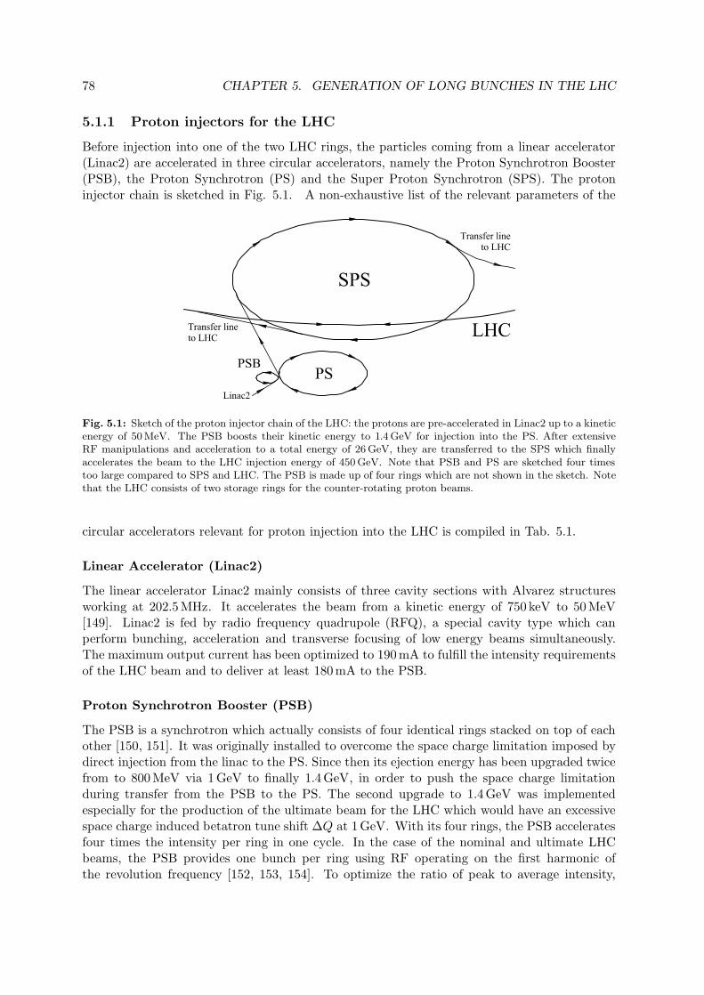
Before injection into one of the two LHC rings, the particles coming from a linear accelerator(Linac2) are accelerated in three circular accelerators, namely the Proton Synchrotron Booster(PSB), the Proton Synchrotron (PS) and the Super Proton Synchrotron (SPS). The protoninjector chain is sketched in Fig. 5.1. A non-exhaustive list of the relevant parameters of the

Fig. 5.1: Sketch of the proton injector chain of the LHC: the protons are pre-accelerated in Linac2 up to a kineticenergy of 50MeV. The PSB boosts their kinetic energy to 1.4 GeV for injection into the PS. After extensiveRF manipulations and acceleration to a total energy of 26 GeV, they are transferred to the SPS which finallyaccelerates the beam to the LHC injection energy of 450 GeV. Note that PSB and PS are sketched four timestoo large compared to SPS and LHC. The PSB is made up of four rings which are not shown in the sketch. Notethat the LHC consists of two storage rings for the counter-rotating proton beams.

circular accelerators relevant for proton injection into the LHC is compiled in Tab. 5.1.

Linear Accelerator (Linac2)

The linear accelerator Linac2 mainly consists of three cavity sections with Alvarez structuresworking at 202.5MHz. It accelerates the beam from a kinetic energy of 750 keV to 50MeV[149]. Linac2 is fed by radio frequency quadrupole (RFQ), a special cavity type which canperform bunching, acceleration and transverse focusing of low energy beams simultaneously.The maximum output current has been optimized to 190mA to fulfill the intensity requirementsof the LHC beam and to deliver at least 180mA to the PSB.

Proton Synchrotron Booster (PSB)

The PSB is a synchrotron which actually consists of four identical rings stacked on top of eachother [150, 151]. It was originally installed to overcome the space charge limitation imposed bydirect injection from the linac to the PS. Since then its ejection energy has been upgraded twicefrom to 800MeV via 1GeV to finally 1.4GeV, in order to push the space charge limitationduring transfer from the PSB to the PS. The second upgrade to 1.4GeV was implementedespecially for the production of the ultimate beam for the LHC which would have an excessivespace charge induced betatron tune shift ∆Q at 1GeV. With its four rings, the PSB acceleratesfour times the intensity per ring in one cycle. In the case of the nominal and ultimate LHCbeams, the PSB provides one bunch per ring using RF operating on the first harmonic ofthe revolution frequency [152, 153, 154]. To optimize the ratio of peak to average intensity,

5.1. GENERATION OF THE NOMINAL AND ULTIMATE LHC BEAM 79

Machine: PSB PS SPS(four rings)

Circumference, 2πR [m] 157.1 628.3 6911.5(normalized to PS) 1/4 1 11Injection energy, Einj [GeV] 0.05 + E0 1.4 + E0 26.0Ejection energy, Eej [GeV] 1.4 + E0 26.0 450Filling scheme 1bunch 2PSB batches 2/3/4PS bats.Number of bunches, nb 1 4 + 2 −→ 72 144/216/288Bunch spacing, tb [ns] 327 −→ 25 25RF harmonics, h 1+2 7→ 21→ 84 4620Fund. RF frequencies, fRF [MHz] 0.6–1.7 3.1/9.3–10/40 200.4Long. emittance at inj. [eVs] 0.35Long. emittance at ej. [eVs] 1 0.35 0.70Nominal scheme:Beam int. at inj., Ntot 1.87 · 1012 /rg. 9.66 · 1012 1.66/2.48/3.31 · 1013

IL = 180mABeam int. at ejection, Ntot 1.63 · 1012 /rg. 8.28 · 1012 1.66/2.48/3.31 · 1013

Ultimate scheme:Beam int. at inj., Ntot 2.76 · 1012 /rg. 1.43 · 1012 2.45/3.67/4.90 · 1013

IL = 180mABeam int. at ejection, Ntot 2.41 · 1012 /rg. 1.22 · 1013 2.45/3.67/4.90 · 1013

Tab. 5.1: Relevant parameters of the circular accelerators in the LHC injector chain.

a second harmonic RF system is used to flatten the bunches and thus to decrease the peakintensity [155, 156]. For the LHC beam each PSB bunch has an intensity of some 1.6 · 1012

protons, slightly more than twelve times the intensity of an LHC bunch because of losses duringtransfer and capture in the PS. The transfer between the four rings of the PSB and the PS issketched in Fig. 5.2. During the first transfer, bunches from all four booster rings are stringed

Fig. 5.2: Double batch transferscheme from PSB to PS. For the in-jection into the PS all four boosterrings are used, each delivering onebunch. The second injection is per-formed with two booster bunchesonly.

up in the PS. One PSB machine cycle later (corresponding to 1.2 s), half of the rings are usedto deliver two more bunches. Finally, six of seven PS buckets are populated. The empty bucketis needed for the transfer from the PS to the SPS to preserve a gap for the beam ejection.

Proton Synchrotron (PS)

The PS is a combined function alternating gradient synchrotron which accelerates the protonbeam to a total energy of up to 26GeV [157, 158, 159]. However, acceleration is not the onlyfunction of the PS in the LHC injector chain [160]. It also has to prepare the bunch structure forthe LHC: bunches with an intensity of slightly more than 1.15·1011 protons with a bunch spacingof 25 ns. Successive longitudinal splitting procedures are performed to meet these requirements.


The longitudinal emittance at ejection from the PS must be around 0.35 eVs, much below thefinal nominal emittance of 2.5 eVs in the LHC, to fit the bunches into the rather small bucketsof the 200MHz RF system in the SPS.

As the six bunches coming from the PSB are injected at h = 7, the bunch spacing atfinal energy would be some 300 ns, and the longitudinal emittance would be much too largeto capture these bunches in the SPS. Therefore each bunch is split into twelve equal fractions,which reduces the longitudinal emittance per bunch to a value that is acceptable for the SPS.The bunch spacing is also divided by twelve to the nominal LHC parameter of 25 ns. Thesplitting factor can be decomposed to 12 = 3 · 2 · 2, so that one triple-splitting and two bunchpair splittings are performed (see Sec. 3.2.2). To keep the RF frequencies during accelerationwithin the capabilities of the main RF system in the PS (2.8 to 10MHz) [161, 162], the triplesplitting is initiated during the injection flat-bottom at 1.4GeV [163]. Thereafter the beam isaccelerated on h = 21 and subsequently the bunches are split twice to h = 42 and finally toh = 84. The RF gymnastics for the preparation of the LHC beam in the PS is illustrated inFig. 5.3. Finally one ends with a batch of 72 bunches and, as the empty bucket splits exactly

Fig. 5.3: Acceleration and bunch splitting scheme of the nominal LHC beam in the PS. Starting from 4 + 2bunches from the PSB each of them is split twelve times in total so that on ends up with a batch of 72 bunchesat h = 84 with 25 ns. The empty bucket is also multiplied, and the gap is therefore 12 bunch positions long.

like the bunches, a gap of 12 non-populated buckets. This gap is sufficiently long to allow theextraction kicker magnet to be switched on without perturbing the beam.

However, the bunches after the last double bunch splitting are held with some 100 kV at40MHz, where their bunch length of 12 ns is still too long to fit into the SPS 200MHz buckets.Since the voltage required in the PS to shorten them adiabatically would be unreasonably large,a non-adiabatic rotation (see Sec. 3.3.1) of the bunches in the longitudinal phase space is usedfor bunch compression before extraction [164, 165]. By rapidly switching the RF amplitude at40MHz (h = 84) to 300 kV and additionally applying some 600 kV at 80MHz (h = 168), thebunch length is reduced to 4 ns [166] after some 600 turns in the PS, well below the bucketlength of 5 ns in the SPS. Fast extraction delivers the batch of 72 bunches to matched 200MHzbuckets in the SPS.


Super Proton Synchrotron (SPS)

The batches coming from the PS are accumulated and accelerated in the SPS up to the injectionenergy of the LHC at 450GeV. As mentioned in App. A, the SPS is a separated functionalternating gradient synchrotron [167] equipped with a special traveling wave RF system foracceleration. Its circumference of 6.9 km is exactly eleven times as long as the circumference ofthe PS. However, eleven PS batches consisting of 72 bunches cannot be accelerated in the SPSbecause the total beam intensity is presently limited to some 5 · 1013 by the maximum powerthat can be transferred to the proton beam during its passage through the RF cavities.

Two, three or four PS batches are therefore accumulated at flat-bottom in the SPS, corre-sponding to an intensity of 1.7, 2.5 or 3.3·1013 protons (see Tab. 5.1). No special RF gymnasticsduring the injection procedure is necessary, as the beam is prepared by the PS to fit in matched200MHz buckets. It is worth noting that the whole intensity is confined within 2/11, 3/11 or4/11 of the circumference, and that the RF power must be delivered to the beam within thisfraction of the revolution period during each turn.

After an injection flat-bottom of some 3.6/7.2/10.8 s, the beam is accelerated to 450GeVwithin some 8.3 s and ejected to the LHC. During acceleration the bunch emittance is inten-tionally blown-up to twice its initial value to avoid longitudinal instabilities. This blow-up ineffective longitudinal emittance is achieved by either introducing noise to the RF amplitude at200MHz or by an additional RF amplitude at 800MHz, the fourth harmonic of the fundamen-tal RF system [168]. The bunches with nominal intensity have a longitudinal emittance below0.6 eVs at extraction from the SPS [169].

Large Hadron Collider (LHC)

Each of the LHC rings will be filled by 12 injections at 450GeV. The two rings will be equippedwith a superconducting RF system consisting of eight cavities per ring that are capable to deliverup to 16MV to the beam [170]. As the 400.8MHz buckets in the LHC cannot be exactly matchedto the bunch length to energy spread ratio of the injected bunches, a longitudinal emittanceblow-up of some 25% to 0.8 eVs hast to be accepted. On the one hand, the maximum voltageof the 200.4MHz RF system is not enough to match the beam to the LHC buckets, and on theother hand, the RF voltage in the LHC cannot be lowered because of insufficient bucket area.A detailed analysis of the injection procedure can be found in [118].

After injection, the two beams are accelerated to the collision energy of 7TeV. As longitu-dinal instabilities are expected during acceleration for low-emittance bunches, the longitudinalemittance is again intentionally blown up to 1 . . . 1.5 eVs. Due to the long ramping time of20min that is limited by the ramp rate of the superconducting magnets, acceleration takesplace at a moderate rate of 485 keV/turn.

The expected final bunch parameters at 7TeV, which are the basis for the RF gymnasticsfor long and flat bunches, are presented in Fig. 5.4 and Tab. 5.2. The longitudinal emittanceof the bunches will be deliberately blown up to 2.5 eVs during acceleration to prevent fromunwanted emittance dilution due to intra-beam scattering at collision energy. However, 1 eVsat the end of the acceleration cycle should be within reach.

It should be mentioned that synchrotron radiation can be neglected for the calculation of thenominal bunch parameters. Although it is important for the heat load on the superconductingmagnets, the average energy loss as calculated in Sec. 2.8 is with 6.71 keV per turn negligiblecompared to the external RF voltage of 16MV. The resulting synchronous phase angle becomesφ0 = (180 − 0.024)0.


-1 -0.5 0 0.5 1t @nsD

-2

-1

0

1

2

DE

@GeVD

Fig. 5.4: LHC bunch at 7TeVenergy with εl = 1.5 eVs.

Small emittance NominalBucket area, A 7.62 eVsBucket length 0.748m (2.5 ns)Bucket height 2.4GeVLong. emittance, εl 1.0 eVs 2.5 eVsBunch length 0.20m (0.66 ns) 0.32m (1.08 ns)Energy spread 0.97GeV 1.51GeV(relative) (0.13 · 10−3) (0.22 · 10−3)Peak current (par.) 42.3A 26.5A

Tab. 5.2: Relevant parameters of a nominal LHC bucket and bunchwith a longitudinal emittance of 1.0 or 2.5 eVs.

Nominal bunch pattern in the LHC

For the filling of one LHC ring, twelve SPS cycles containing three or four PS batches each willbe required. At a bunch spacing of 25 ns the LHC has 3564 possible bunch positions, but not allof these bunch positions can be populated by a bunch, as there are several restriction imposedby the injector chain as presented above and by the LHC itself [171, 172]:

Firstly, the transfer of multiple batches from PS to SPS demands for a gap of at least 8bunch positions as the SPS injection kicker magnet needs to be switched on between subsequentbatches. It should be mentioned that the gap between two batches in the SPS is shorter thanthe extraction kicker gap in PS. Secondly, a gap of 38 or 39 empty bunch positions, dependingon the number of PS batches delivered from the PS, must be provided for the injection kickermagnet in the LHC. The largest gap in the LHC bunch pattern assigns the time for the so-calledbeam dump kicker. As this kicker magnet must be activated at the collision energy of 7TeV,its rise time is significantly longer than those of the kicker magnets considered above. At least119 bunch positions (3µs) must be kept free from particles to allow save abort of beam at fullenergy to the dump.

Various bunch patterns for the different operation modes, i.e. different bunch spacing orions instead of proton beams, have been analyzed. As an example for a standard bunch pattern,the nominal filling scheme for high luminosity operation with 25 ns bunch spacing is describedbelow. The filling procedure is sketched in Fig. 5.5. Following the bunch pattern notation

Fig. 5.5: Nominal filling scheme from PS to LHC for luminosity production with 25 ns bunch spacing. Thebunch patterns in SPS and LHC are drawn to scale whereas the PS bunch pattern is magnified.


in [173, 174] where b denotes a populated bucket and e an empty bunch position, the fillingscheme in the PS can be simply written as

fsPS ⊕ 4⊗ e = (72 ⊗ b⊕ 8⊗ e)⊕ 4⊗ e ,

so that fsPS denotes the PS bunch pattern that reappears in SPS and LHC (see Fig. 5.5, topleft). The operators marked by a circle can be regarded as non-commutative additions andmultiplications. The pattern in the SPS can be composed of a string of PS patterns and ofpadding with empty buckets to end up with 924 possible bunch positions.

The full bunch pattern in the LHC can be described by the a sequence of digits defining thenumber of PS batches per SPS cycle, namely

234 334 334 334 .

Resolving this pattern according to the notation introduced above, the full nominal fillingscheme for the LHC becomes

fsLHC = 2⊗ fsPS ⊕ 30 ⊗ e⊕ 3⊗ fsPS ⊕ 30⊗ e⊕ 4⊗ fsPS ⊕ 31⊗ e⊕ 3⊗ 2⊗ [fsPS ⊕ 30⊗ e]⊕ 4⊗ fsPS ⊕ 31⊗ e ⊕ 80⊗ e ,

where the curly brackets are set corresponding to the bunch pattern above. The complete fillingscheme can thus be written as

fsLHC = 2⊗ (72 ⊗ b⊕ 8⊗ e)⊕ 30⊗ e⊕ 3⊗ (72 ⊗ b⊕ 8⊗ e)⊕ 30⊗ e⊕ 4⊗ (72 ⊗ b⊕ 8⊗ e)⊕ 31⊗ e

⊕ 3⊗ 2⊗ [3⊗ (72⊗ b⊕ 8⊗ e)⊕ 30⊗ e]⊕ 4⊗ (72⊗ b⊕ 8⊗ e)⊕ 31⊗ e ⊕ 80⊗ e . (5.1)

By setting b and e to unity it can easily been shown that the total number of bunch positionsis 3564. Furthermore, setting b = 1, e = 0 shows that the number of bunches per LHC ring is2808.

The bunch pattern can by modified as long as the bunch train structure fsPS remains un-changed. However, the generation of long bunches in the LHC as described below alreadyrequires modifications of the bunch pattern in the PS.

5.1.2 Limitations of the LHC injector chain

Several limitations of the existing accelerator complex may restrict the performance of an up-graded LHC, as the injector chain will already have a hard time providing the protons requiredfor the ultimate scheme.

At low energy, the total beam intensity is limited by the tune shift induced by the transverseself-field of the beam. The space charge force acts incoherently on the individual particlesdepending on their position inside the beam. A short derivation of the space charge tune shiftis given in App. F. Similar to beam-beam tune spread in high energy colliders, the so-calledspace charge limit is extremely difficult to compensate and, in analogy to the beam-beam limit,it is regarded as the fundamental current limitation for circular hadron accelerators in the lowenergy regime.

Furthermore, extremely high beam intensities may result in a significant radioactive irradi-ation of the accelerators if beam losses are not well under control. As most of the uncontrolled


beam losses take place at low energies where lost particles deposit their energy almost com-pletely within the accelerator components, this is of special concern for the injector chain of theLHC.

Various options for increasing the beam intensity as well as reducing the uncontrolled beamlosses in the LHC injector chain are under discussion [175] to remove its limitations at low beamenergy. Although the maximum bunch intensity within the beam quality requirements for theLHC is presently limited to 1.5 · 1011 protons per bunch (about 20% above the bunch intensityneeded for the nominal LHC scheme) in the PS, especially the installation of a new high energyinjector linear accelerator, the so-called Superconducting Proton Linac (SPL), would increasethe available bunch intensity to some 4 · 1011 protons [175]. This improvement comes from thefact that such a linear accelerator would allow injection into the PS at an energy of 2.2GeVwhere the direct space charge limitation is suppressed by a factor of βγ2|2.2GeV/βγ

2|1.4 GeV ' 1.9compared to the present transfer energy between PSB and PS.

For the further analysis in this report it is assumed that the injector chain does not imposea strict intensity limitation for the LHC, and that it is capable of delivering a beam similar tothe nominal LHC beam but with intensities up to three to four times its bunch population atejection from the SPS.

5.2 Generation of long and flat bunches

Starting from an almost standard LHC beam configuration with 25 ns bunch spacing, differ-ent schemes to confine batches of nominal bunches to long and flat bunches or even singlesuperbunches per beam have been discussed in Chapter 4.

5.2.1 Direct approach

A straightforward approach to form long and flat bunches at flat-top energy in the LHC wouldbe the merging of each PS batch with its length of 72 bunches at a time distance of 25 nseach into one long bunch held by barrier buckets [176]. According to the total number of PSbatches in the LHC, 39 long and flat bunches would finally remain. It should be mentionedthat synchrotron radiation is assumed to be properly compensated at 7TeV by a dedicated RFinstallation during the manipulations described below.

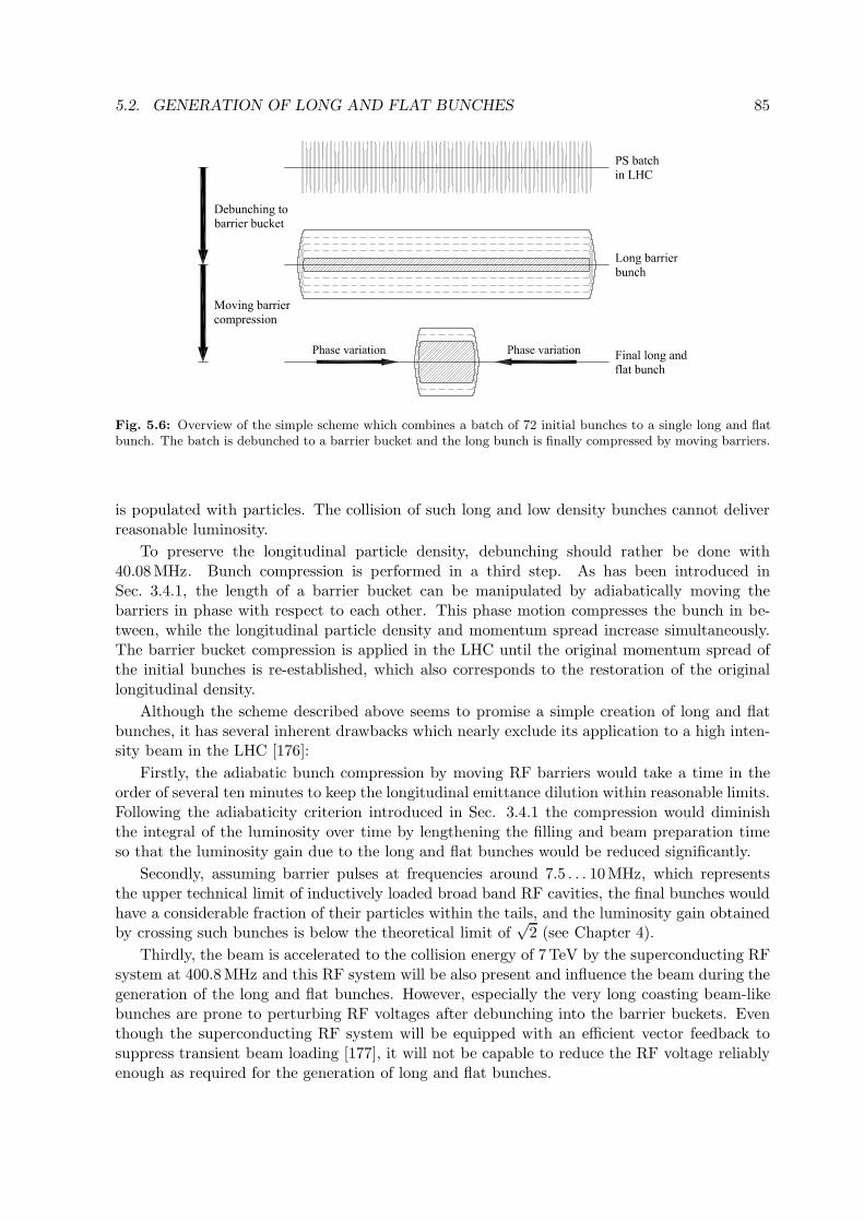
Fig. 5.6 illustrates the longitudinal phase space during the subsequent steps of the scheme.Before the generation of long and flat bunches, the beam is injected and accelerated according tothe scheme for the nominal LHC beam. At the injection flat-top, barrier buckets are positionedin the 9 · 25 ns = 225ns long gaps between two adjacent PS batches in a first step. In a secondstep the amplitude of the harmonic RF system holding the beam is decreased adiabaticallyso that the bunch trains are debunched to the barrier bucket placed around the batch. Thisdebunching procedure can be performed either directly starting from the 400.8MHz RF system,or the bunches could be handed over to an RF system at 40.08MHz. An RF system at 40.08MHzwould be compatible with the nominal bunch spacing of 25 ns and could serve as a mediatorbetween the 400.8MHz RF buckets and the RF barriers pulses whose pulse length correspondsto a frequency of some 10MHz.

After debunching, coasting beam-like flat bunches with a length of approximately 1.8µs areconfined by the barrier pulses (Fig. 5.6, center). It is worth mentioning that debunching with400.8MHz would lead to a much reduced longitudinal density because only every tenth bucketat an RF frequency is occupied in the nominal scheme so that less than 10% of the batch length

5.2. GENERATION OF LONG AND FLAT BUNCHES 85

Fig. 5.6: Overview of the simple scheme which combines a batch of 72 initial bunches to a single long and flatbunch. The batch is debunched to a barrier bucket and the long bunch is finally compressed by moving barriers.

is populated with particles. The collision of such long and low density bunches cannot deliverreasonable luminosity.

To preserve the longitudinal particle density, debunching should rather be done with40.08MHz. Bunch compression is performed in a third step. As has been introduced inSec. 3.4.1, the length of a barrier bucket can be manipulated by adiabatically moving thebarriers in phase with respect to each other. This phase motion compresses the bunch in be-tween, while the longitudinal particle density and momentum spread increase simultaneously.The barrier bucket compression is applied in the LHC until the original momentum spread ofthe initial bunches is re-established, which also corresponds to the restoration of the originallongitudinal density.

Although the scheme described above seems to promise a simple creation of long and flatbunches, it has several inherent drawbacks which nearly exclude its application to a high inten-sity beam in the LHC [176]:

Firstly, the adiabatic bunch compression by moving RF barriers would take a time in theorder of several ten minutes to keep the longitudinal emittance dilution within reasonable limits.Following the adiabaticity criterion introduced in Sec. 3.4.1 the compression would diminishthe integral of the luminosity over time by lengthening the filling and beam preparation timeso that the luminosity gain due to the long and flat bunches would be reduced significantly.

Secondly, assuming barrier pulses at frequencies around 7.5 . . . 10MHz, which representsthe upper technical limit of inductively loaded broad band RF cavities, the final bunches wouldhave a considerable fraction of their particles within the tails, and the luminosity gain obtainedby crossing such bunches is below the theoretical limit of

√2 (see Chapter 4).

Thirdly, the beam is accelerated to the collision energy of 7TeV by the superconducting RFsystem at 400.8MHz and this RF system will be also present and influence the beam during thegeneration of the long and flat bunches. However, especially the very long coasting beam-likebunches are prone to perturbing RF voltages after debunching into the barrier buckets. Eventhough the superconducting RF system will be equipped with an efficient vector feedback tosuppress transient beam loading [177], it will not be capable to reduce the RF voltage reliablyenough as required for the generation of long and flat bunches.


Fourthly, the effect of the average energy loss of the particles at collision energy caused bysynchrotron radiation must be compensated. This requires an RF system generating a constantvoltage of some 6.7 kV along the full PS batch length of 1.8µs. As the RF systems have to befree from of DC components, the long positive pulse must be followed by a short negative pulseof large amplitude which is generated within the gap of two PS batches. Such a compensation,which is necessary in addition to the barrier bucket system to confine the long bunches, presentsa challenging and expensive task.

Finally, the momentum spread after debunching to the barrier bucket is small comparedto the spread of the nominal LHC bunches. The thresholds for the microwave instability (seeChapter 6) are therefore much below the estimated longitudinal impedance in the LHC. As aresult, the beam is unstable during the creation of the long and flat bunches.

These major disadvantages of the straightforward scheme of long bunch generation in theLHC demand new approaches to perform the necessary RF manipulations. A more promisingscheme is therefore presented below.

5.2.2 Overview of the long bunch generation scheme

The RF gymnastics to generate long and flat bunches, about one order of magnitude longer thanthe nominal LHC bunches, mainly consists of three ingredients. Two of them, batch compressionand bunch pair merging, have been briefly introduced in Chapter 3. The third ingredient, thefinal formation of the long and flat bunch, is very similar to a bunch pair merging with threeor more harmonics which is just stopped in the middle of the process.

Batch compression serves to increase the harmonic number in a circular accelerator fromh1 to h2. The difference of the two harmonics is chosen small enough so that the bunchescan follow the buckets during the harmonic hand-over (see Sec. 3.2.3). The bunch spacingdecreases and it is therefore used to push the batches of bunches together more closely. In thenominal LHC scheme, only every tenth bucket is a possible bunch position. Starting the batchcompression at the nominal RF harmonic of h = 35640 would be inconvenient, because thenumber of empty buckets between two bunches remains the same. Therefore, the generationof long and flat bunches starts from an RF system at ten times lower RF harmonic h = 3564(40.08MHz), where every bucket serves as a bunch position. Stepwise increase of the harmonicnumber up to h = 7128 (80.16MHz) causes the bunch spacing to shrink by a factor of two to12.5 ns, whereas the number of bunches stays constant throughout the procedure.

To re-establish the original bunch spacing and to reduce the number of bunches, the com-plementary procedure, bunch pair merging, is applied where the RF amplitude at h = 7128 isadiabatically decreased while simultaneously increasing the amplitude at h = 3564. The bunchspacing increases again to 25 ns but the number of bunches is halved with respect to the initialstate.

Repetitive application of this sequence of batch compression and bunch pair merging allowsto progressively confine dense bunches as illustrated in Fig. 5.7. It is obvious that thenumber of initial bunches must be a power of two so that the confinement is restricted to4, 8, 16, 32, 64 . . . 2n bunch batches. A reasonable choice of this batch length is explained inwhat follows.

Choice of batch length

Two main arguments determine the number of initial bunches to be combined to one long andflat bunch in the LHC:


Fig. 5.7: Subsequent application of batch compression and bunch pair merging gradually reduces the numberof bunches and increases the intensity per bunch.

Firstly, assuming a constant emittance per bunch, the required RF voltage for the creationand the storage of the long and flat bunches is proportional to the square of the numberof combined bunches. The absolute voltages necessary to store the final bunches after thecombination of batches of 16 bunches can be found in Tab. 4.3. A reasonable RF voltageproviding sufficient bucket area during the creation of these bunches is somewhat larger, namelyabout 1.5MV.

Secondly, the number of remaining bunches, multiplied by their bunch length, can be con-sidered as an effective beam length. Following the derivations in Sec. 4.2.5, this effective beamlength nblb should be chosen so that the maximum beam-beam tune shift is reached with themaximum available average beam current (see Fig. 4.3).

The relevant beam parameters for different numbers of bunches confined to one long bunchare given in Tab. 5.3.

Number of initial bunches 1 4 8 16 32 64per long and flat bunchTotal number of bunches, nb 2808 624 312 156 78 39Effective beam length, nblb [m] 531 2613 1306 653 327 163(rectangular equivalent, 3 harmonics)Average current for ∆Q = −0.01, I0 [A] 0.94 12.8 6.4 3.2 1.6 0.8(alternate beam crossings)RF voltage for the generation [MV] 0.1 0.4 1.5 6 24of long bunches, URF

Tab. 5.3: Parameters for the choice of the number of initial bunches to generate a long and flat bunch. Thelongitudinal emittance per initial bunch is taken to be 1 eVs at the LHC injection flat-bottom. The total numberof long and flat bunches per beam is based on the empty to occupied bucket factor 2808/3564 of the nominalLHC beam.

As already pointed out in Sec. 4.3.6, a very high luminosity could be achieved with optionsconfining less than 16 initial bunches, but at the expense of excessively high and unpracticaltotal beam currents.

On the other hand, compressing more than 32 LHC bunches requires a considerable RFvoltage to generate the long bunches, and the beam-beam limit restricts the beam intensity inthe range of the intensity of the ultimate LHC scheme (see Tab. 4.2). However, it will be verydifficult for the experiments to cope with the event rate associated with this very small number


of superbunches in the LHC.Therefore, the only remaining two options of combining either 16 or 32 almost nominal LHC

bunches to one long bunch are considered realistic and worth being discussed in more detail.

Total batch length in the LHC

Direct batch compression of batches of 16 or 32 bunches close to each other without any gapin between is excluded for two reasons: firstly, because the harmonic number 3564 is neitherdivisible by 16 nor 32, and secondly because, during batch compression, the effective RF ampli-tude is modulated along the batch so that at least the edge buckets cannot be populated withparticles.

As the harmonic number h = 3564 decomposes to 22 · 34 · 11, the favorable batch lengthsleaving at least one empty bucket at each end are nbatch = 2 · 32 = 18 for 16 respectivelynbatch = 22 · 32 = 36 for 32 bunches. The fundamental harmonic of the batch confinementRF gymnastics is thus 198 or 99 which corresponds to the number of available bunch positionsfor the final long and flat bunches. Furthermore, the step width in harmonic number of thehand-overs during batch compression is also defined by this step of ∆h = 198 or ∆h = 99.

The complete schedule for the harmonic number changes during batch compression as wellas the increase of the number of buckets per batch is illustrated in Figs. 5.8 and 5.9. The bunch

nbatch Pattern h Merge18 16⊗ b⊕ 2⊗ e 3564 3564

19?

16⊗ b⊕ 3⊗ e?

3762+198?

20?

16⊗ b⊕ 4⊗ e?

3960+198?

· · ·? · · ·? · · ·?

36?

16⊗ b⊕ 20⊗ e?

7128?

- 7128

/2

6

Fig. 5.8: Schedule of harmonic numbers and bunchpatterns during long bunch combination of 16 initialbunches.

nbatch Pattern h Merge36 32⊗ b⊕ 4⊗ e 3564 3564

37?

32⊗ b⊕ 5⊗ e?

3663+99?

38?

32⊗ b⊕ 6⊗ e?

3762+99?

· · ·? · · ·? · · ·?

72?

32⊗ b⊕ 40⊗ e?

7128?

- 7128

/2

6

Fig. 5.9: Same harmonic schedule as in Fig. 5.8 butfor a batch of 32 initial bunches. The bunch patternnotation is introduced at the end of Sec. 5.1.1.

patterns are given for the first batch compression. For subsequent compressions the number ofbunches is less while the number of empty bucket positions is larger.

It can be seen from the harmonic schedule that the RF systems for the batch compressionhave to cover the frequency range from 40.08 (h = 3564) to 80.16MHz (h = 7128), no matterwhether 16 or 32 bunches are combined. However, no more than two RF harmonics are actingon the beam simultaneously so that the complete RF gymnastics can be covered by two tunablegroups of RF systems. It should be mentioned that the final formation of the long and flatbunches may require additional fixed frequency RF systems if more than two harmonics areapplied to flatten the bunch shape.


The new LHC cycle

At the collision energy of 7TeV, each beam with nominal intensity contains some 362MJ(2808 · 1.15 · 1011 protons), which makes the machine extremely sensitive to any kind of beamlosses. At injection energy, the acceptable losses are 15 times larger. As complicated RFgymnastics can cause small beam losses, it is clearly preferable to perform most of the beamgymnastics at the injection flat-bottom of the LHC.

Neglecting the effects of bucket area reduction during batch compression, a change of theharmonic number at constant RF voltage causes the bucket area to shrink according to 1/h3/2

so that the smallest bucket area occurs at the end of the batch compressions. The bucket areafor relevant harmonic numbers together with the bunch emittances are shown in Fig. 5.10. It

3564 4158 4752 5346 5940 6534 7128Harmonic number

5

10

15

20

25

30

35

40

A@eVsD

32 bunches

16 bunches

8 bunches

4 bunches

6.0 MV

1.5 MV

LHC, 450 GeV

Fig. 5.10: Bucket area versus harmonicnumber for relevant RF frequencies be-tween 40.08 and 80.16 MHz at constantvoltage of 1.5 and 6MV at the injec-tion flat-bottom in the LHC. The dashedlines show the total emittance of 2n initialbunches.

becomes clear that in the 16 bunch scheme as well as in the 32 bunch scheme the initial batchcan be combined to two remaining buckets held at h = 3564 at injection energy.

While the bunch emittance stays virtually constant during acceleration, the bucket areagrows proportionally to

√E/|η| ' γtr

√E ∝ √E so that it is 3.9 times larger at collision energy.

Therefore the last batch compression and the final formation of the long and flat bunches mustbe carried out at the LHC flat-top.

Batches of two bunches according to the bunch pattern of 2⊗b⊕16⊗e (16 initial bunches) or2⊗b⊕34⊗e (32 initial bunches) are accelerated with the 40.08MHz RF system. The moderateaverage energy gain of 485 keV/turn results in a synchronous phase of φ0 = (180 − 18.8)0

respectively (180 − 4.6)0, and the bucket area reduction as sketched in Fig. 2.5 due to thesynchronous phase is not critical during acceleration.

It is important to point out that an additional benefit of shifting as much of the RF manip-ulations to the injection flat-top is offered by the scaling of the synchrotron frequency propor-tional to

√|η|/E ' 1/(γtr

√E) ∝ 1/

√E. To keep the same adiabaticity during the process, the

manipulation can be executed four times faster at 450GeV.


5.2.3 Beam transfer from SPS to LHC

As the batch confinement RF gymnastics is based on RF systems at harmonic numbers between3564 and 7128, the beam from the SPS is injected into large 40.08MHz buckets at the LHCflat-bottom. Furthermore, the estimation of the beam loading voltage induced to the supercon-ducting 400.8MHz cavities (see Sec. 6.5) shows that they even have to be removed for operationwith long bunches. Parallel operation of both the standard superconducting RF system and a40.08MHz RF installation is impossible with reasonable power capabilities.

The condition for a longitudinally matched bunch to bucket transfer between two circularaccelerators has been derived in Sec. 3.5 so that the voltage ratio optimum between SPS andLHC is given by

VSPS

VLHC=(RSPS

RLHC

)2 ∣∣∣∣ ηSPS

ηLHC

∣∣∣∣ hLHC

hSPS= 0.38 · hLHC

hSPS. (5.2)

For matched injection into 40.08MHz buckets the voltage ratio becomes 0.29. However, as anadditional constraint, the bucket area must be sufficient in both accelerators.

The bucket area of the 200MHz SPS buckets at extraction flat-top is plotted in Fig. 5.11versus the available RF voltage. Assuming a bunch emittance of 0.6 to 0.7 eVs at 450GeV, the

0 1 2 3 4URF @MV D

0.9

1.3

1.7

2.1

A@eVsD

1.2 eVs

1.8 eVs

SPS, 450 GeV

Fig. 5.11: Bucket area of the 200 MHz RF sys-tem in the SPS versus its RF amplitude.

bucket area should be at least three times as large as the bunch emittance to keep the bunchwithin the linear region of the bucket. Therefore, the minimum RF voltage limitation in theSPS for extraction into a 40.08MHz RF system in the LHC is about 3MV. The upper voltagelimit is simply given by the available RF power, which limits the maximum RF voltage to some8MV.

Beam transfer by bunch rotation

Depending on whether 16 or 32 initial bunches should be combined to one long and flat bunch,the available RF voltage at 40.08MHz in the LHC will be either 2 · 1.5MV or 2 · 6MV.

In the case of 3MV, the corresponding RF voltage in the SPS according to Eq. (5.2) is only0.87MV so that the bucket area would be insufficient. Therefore, a virtual reduction of theRF voltage by bunch rotation is foreseen, to obtain a ratio of bunch length to energy spread ofabout 0.87MV at extraction. The bunches are rotated in the longitudinal phase space in theSPS, and the extraction to the LHC takes place when the bunch length is largest, respectivelyafter a rotation by a quarter of a turn.

Following the analysis in Sec. 3.3.1, the maximum bunch lengthening factor reachable byan instantaneous voltage step down from 8 to 3MV is 1.63. After rotation in the longitudinal


phase plane, when the bunch is longest, it has similar parameters as a bunch kept in a stationarybucket with 1.1MV, except that such a bunch would be significantly stretched out in the non-linear regions of the bucket as its emittance is close to the bucket area (see Fig. 5.11).

Tracking calculations of the beam transfer scheme by bunch rotation show that a small butnon-negligible emittance blow-up occurs. Starting from a matched bunch of 0.65 eVs longitudi-nal emittance in the SPS, the RF amplitude is raised adiabatically from 3MV to 8MV and thensuddenly switched back to 3MV. After one quarter of a period at the synchrotron frequency,the bunch is transferred to the LHC and tracked for further 0.2 s to observe residual mismatch.The longitudinal emittance blow-up caused by such a transfer between SPS and LHC with opti-mized parameters is illustrated in Fig. 5.12. As expected, the longitudinal emittance remains

0 0.1 0.2 0.3 0.4Time @sD

0.2

0.4

0.6

0.8

1

¶ l@eVsD

SPS

200 MHz, 3 to 8 MV200 MHz, 2.48 MV

LHC

40 MHz, 3 MV40 MHz, 12 MV

Fig. 5.12: Longitudinal emittance during abunch transfer from SPS to LHC includingbunch lengthening by bunch rotation in theSPS (continuous line). The dashed line rep-resents the transfer to 12 MV at 40.08 MHzin the LHC. The longitudinal emittance isdefined as the area of the encircling ellipsecontaining 99 % of the bunch particles nor-malized to 0.65 eVs at the beginning of theprocess.

constant during the adiabatic voltage increase within the first 200ms. The bunch rotation itselfis by far too fast to be visible on the timescale of Fig. 5.12; the bunch is extracted some 2.5msafter the instantaneous voltage reduction. After injection into the LHC, an oscillation of theeffective longitudinal emittance with the synchrotron frequency can be observed. It is caused bythe residual longitudinal mismatch of the injected bunch. After filamentation, the final bunchhas an emittance of some 0.8 eVs and the transfer blow-up is about 23%. It should be pointedout that the residual longitudinal mismatch comes from a non-ideal bunch rotation: a signif-icant fraction of particles suffers from the reduced synchrotron frequency at large oscillationamplitudes. Therefore, the optimum rotation time must be 1.25 · π/(2ωs) to obtain minimumtransfer blow-up, slightly longer than a quarter period of the linear synchrotron frequency.

Direct transfer

In the case of 32 initial bunches combined to one long and flat bunch, the available RF voltagehas to be about 2 · 6MV at 40.08MHz and, according to Eq. (5.2), the corresponding RFvoltage in the SPS is about 3.5MV. It is expected that the matched transfer causes virtuallyno longitudinal emittance blow-up (see Fig. 5.12, dashed line).

However, the bucket area of a 40.08MHz RF system in the LHC is much larger than theemittance of the injected bunches resulting in low synchrotron frequency spread and virtuallyno Landau damping. This might restrict the maximum RF amplitude during injection, and thebunch rotation scheme might be favorable even if more RF voltage would be available.

Albeit the ideal longitudinal emittance after beam transfer to the LHC is estimated to bebelow 0.8 eVs, an additional blow-up caused by a higher harmonic RF system to re-establish


Landau damping (see Sec. 6.3.6) must be taken into account. Therefore the subsequent analysisof the RF gymnastics assumes a longitudinal emittance of 1 eVs.

It is important to point out that the transfer of nominal bunches from the SPS (8MV)to the 400.8MHz RF system (8MV) also causes a longitudinal emittance blow-up. Instead ofstretching the bunches as suggested above, a bunch rotation might be an option to shorten thebunches and to suppress the mismatch [178].

5.2.4 Batch compression

After beam injection, the RF manipulation to generate the long and flat bunches commences.The harmonic number is raised in steps of 198, respectively 99, which corresponds to a stepof unity with respect to the local harmonic number of the batch (see Figs. 5.8 and 5.9). Thelower harmonic RF amplitude at h1 is adiabatically decreased while the higher harmonic RFat h1 + 198 or h1 + 99 is increased simultaneously.

When both harmonics are of equal RF voltage, the beat frequency at h2 − h1 has the sameamplitude as the two main carriers so that the effective RF focusing is large at the center ofthe batch but decreases to nearly zero at the very ends of the batch. This problem is mostcritical at the beginning of the first harmonic hand-over as only the last (16 initial bunches) orthe last two (32 initial bunches) buckets are kept empty at both ends of the batch. An exampleof the separatrices and bucket areas for the worst case during the first harmonic hand-over ofthe combination of 32 bunches is shown in Fig. 5.13. In the case of 16 initial bunches, the

0 Π4 Π2 3Π4 ΠΦ @radD

-1

0

1

DE

@GeVD 36.8 36.5 36.1 35.6 34.9 34.1 33.1 32.0 30.7 29.3 27.7 25.9 23.8 21.5 18.8 15.7 11.8 6.0

Fig. 5.13: Separatrices in the middle of the first harmonic hand-over from h = 3564 to 37/36 · 3564 = 3663when both RF voltages are equal and at half of their maximum amplitude, namely 3MV each. The separatricesof empty buckets are plotted with dashed lines. As the stationary trajectories are symmetric around φ = 0 onlyone half is shown. The buckets areas (in the center of the separatrices) are given in units of eVs.

situation is similar. The bucket area of the populated buckets varies from 8.1 to 17.9 eVs inthis case, and the empty bucket at the end of batch has an area of 4.1 eVs.

The analysis above seems to suggest that the gaps in between the batches are not mandatory.However, despite of their function to make the bunch pattern compatible with the LHC withits global harmonic of 3564, it is important to point out that the bucket area dynamicallyoscillates from the stationary value as shown in Fig. 5.10 to the minimum value (Fig. 5.13)within each single harmonic hand-over. In the adiabatic limit, the bunch inside the bucket mustbe able to follow this quadrupole excitation caused be the bucket motion without dilution inthe longitudinal phase space. The development of the bucket areas of center (dashed line) andtail buckets is presented in Figs. 5.14 and 5.15. While the area of the center bucket shrinkssmoothly, the outer buckets, especially the last one, are strongly modulated. This behaviour


0.0 0.2 0.4 0.6 0.8 1.0Time @a.u.D0

10

20

30

40

A@eVsD

LHC, 450 GeV, bunch #1 and #18

Fig. 5.14: Development of the bucket area duringbatch compression from h = 3564 to 7128 in steps of∆h = 99. While the center bunch mainly shrinks pro-portional 1/h3/2 (dashed line), the last bunch showsa strong modulation of the bucket area with each har-monic hand-over (continuous).

0.0 0.2 0.4 0.6 0.8 1.0Time @a.u.D0

10

20

30

40

A@eVsD


Fig. 5.15: Comparison of the bucket area de-velopment of center (dashed line) and last popu-lated bucket (continuous). The bucket area is stillstrongly modulated, but the variation is already sig-nificantly reduced compared to the last, empty bucket(Fig. 5.14).

can cause emittance dilution if the bucket area is modulated so fast that the bunch is not ableto follow the rapid changes of the bucket.

For the calculation of Figs. 5.14 and 5.15 the time for each harmonic hand-over was assumedto be constant. Since the degree of modulation is largest for the first sub-steps of the batchcompression, they should be lengthened so that the time derivative of the effective RF focusingdoes not surpass a certain limitation during the batch compression manipulation.

Time optimization

From the analytical calculation of RF potential or separatrices during batch compression, onecould get the impression that the RF manipulation is symmetric in the sense that both ends ofthe batch move to the center simultaneously. However, it should be kept in mind that, abovetransition, the bunch at the front of the batch must be slightly accelerated while the bunch atthe back must be decelerated to initiate their relative phase motion with respect to the batchcenter.

Therefore a batch compression can also be regarded as sketched in Fig. 5.16. Each

Fig. 5.16: During batch compression, each bunch of the batch has to be slightly accelerated or decelerated tomove them towards the center. The offset energy of this acceleration or deceleration increases with the distanceof the bunch from the center of the batch.

bunch is slightly displaced in energy where it drifts in phase to reach its new position after the


batch compression. It becomes clear that the bunch motion of the front and the back half arereflections in a point around the batch compression center.

It is worth noting that this view of the batch compression manipulation is not taken intoaccount in the calculations of buckets via the Hamiltonian theory. A simple harmonic hand-over between two harmonics, where the lower harmonic is decreased linearly while the higherharmonic is also increased linearly, the motion of the bucket center switches non-adiabaticallyfrom dφ0/dt = 0 to dφ0/dt 6= 0. This effect excites a dipole oscillation of the bunch, whichcauses emittance dilution and thus a blow-up of the effective longitudinal emittance. Especiallythe bunches at the tails of the batch suffer from this effect.

Therefore, a simple equilibration of the voltage ramps is presented in what follows. Thisequilibration ensures that the bunches are slowly accelerated and decelerated at the beginningand at the end of the batch compression.

For the optimization, the following parameters are assumed at the beginning and at the endof the batch compression:

before afterHarmonic, h h0 −→ 2h0

Total batch length, l l0 −→ l0/2Time, t 0 −→ τbc .

For simplicity it is assumed that the harmonics number does not change stepwise, but thatthe effective harmonic number varies smoothly with time, namely

h(t) = h0

(t

τbc+ 1), (5.3)

so that the length of the batch develops according to

l(t) = l0

/(t

τbc+ 1). (5.4)

This function has a gradient at t = 0 and t = τbc so that the buckets switch from stationaryto moving instantaneously, which is strongly non-adiabatic. Especially at the beginning of theprocess a large energy offset of the tail bunches is required.

An optimized function of the time dependent bunch length l(t) should be smooth and havevanishing derivatives at t = 0 and t = τbc. Trigonometric functions can fulfill these requirements,and a reasonable choice can be written as

lopt(t) =[34

+14

cos(πt

τbc

)]l0 . (5.5)

The improved batch length function is plotted in Fig. 5.17. One can observe that the batchlength starts to shrink smoothly.

The time scaling function to achieve the improved batch length shrinkage can be foundeasily by demanding that lopt(t) = l(t1), where t1 is the new time function which itself dependson the original time t. Finally, this function becomes

t1(t) =[

13/4 + 1/4 · cos(πt/τbc)

− 1]τbc . (5.6)

The time function can be used to convert the linear amplitude ramp functions of the batchcompression to such amplitude where the end of the batch moves according to Eq. (5.5).


0 Τbc2 Τbc

Time

0

l02l0

Bat

chle

ngth

lHtL loptHtLFig. 5.17: Improved batch length function versustime (continuous line). As a reference, the batchlength function of a non-equilibrated batch compres-sion is also shown.


T

ime

@a.u.D

Fig. 5.18: Movement of the bucket centers during the first batch compression for a simple scheme. The thicklines mark the center positions of the buckets while the shaded areas enclosed by thin lines represent the totallongitudinal extent of the buckets. Only one half of the batch is shown.


T

ime

@a.u.D

Fig. 5.19: Same representation of bucket centers and bucket lengths as in Fig. 5.18 but for an improved schemewith a batch length variation according to Eq. (5.5).

The resulting movement of the buckets in the case of non-equilibrated voltage ramps duringbatch compression of 16 bunches is sketched in Fig. 5.18, while the optimized case is presentedin Fig. 5.19. Clearly, especially the edge bunches are accelerated respectively deceleratedsmoothly at the beginning and at the end of the batch compression.

The harmonic program and the RF amplitude ramps for an equilibrated batch compression ofa batch of 16 bunches with 2 empty buckets in between are illustrated in Fig. 5.20. Essentiallythe first and the last harmonic hand-over from h = 3564 to 3564+198 and from h = 7128−198to 7128 have to be performed with non-linear amplitude ramps because the acceleration and


0 2 4 6 8 10Time @sD

3564

4158

4752

5346

5940

6534

7128

0

0.2

0.4

0.6

0.8

1

Am

plitu

[email protected]

Har

mon

ic

40.1

46.8

53.4

60.1

66.8

73.5

80.2

RF

freq

uenc

y@MHzD

1 2 3 4 5 6 7 8 9

10 11 12 13 14 15 16 17 18

Hand-over:

Fig. 5.20: Harmonic and voltage ramps for an optimized batch compression of the bunch pattern 16⊗ b⊕ 2⊗ efrom h = 3564 to 7128 by 18 stepwise harmonic hand-overs. The lower harmonic and the related amplitude areplotted as continuous lines while the higher harmonic and amplitude are represented as a dashed line.

deceleration of the tail bunches needs to be initiated. The intermediate harmonic hand-oversstill have almost linear variation of the RF amplitudes; they are just shifted together in time.

Tracking studies demonstrate the effect of the equilibration during batch compression onthe longitudinal emittance: Figs. 5.21 and 5.22 show the development of the longitudinal RMSemittance during the first batch compression of a batch of 16 bunches with a gap of two emptybuckets between adjacent batches. The initial bunches have a parabolic distribution with atotal emittance of 1 eVs. Each of them consists of some 2000 macro particles. Collective effectsare not taken into account. In the case of a constant time for each harmonic hand-over, theemittance of the tail bunch is diluted significantly due to the non-adiabatic modulation of theRF focusing. It is worth noting that the subsequent bunch mergings become asymmetric evenif only the last bunch suffers from this excitation. This leads to additional emittance dilution.However, in the case of the equilibrated batch compression with amplitude ramps according toFig. 5.20, virtually no longitudinal emittance dilution is visible although the batch compressionhas the same total duration as assumed in the non-optimized case.

Amplitude modulation

It is shown in Fig. 5.13 that the effective RF focusing is strongly modulated along the batchwhen the two RF system acting on the beam have the same amplitude. This modulation,from which especially the tail buckets may suffer, has a negative effect on the bunches at theends of the batch because, as mentioned above, the fast variation in RF focusing can excite aquadrupole oscillations if the RF manipulation is not perfectly adiabatic. The possible benefitof an additional amplitude modulation to counteract the bucket area variation along the batch


0 2 4 6 8 10Time @sD

0.20

0.25

0.30

¶ RM

S@eVsD

Bunch 1 HcenterLBunch 7

Bunch 8 HtailL

Fig. 5.21: Emittance development of center andtail bunches during batch compression of a 16 bunchbatch in the LHC from h = 3564 to 7128. Each har-monic hand-over has the same duration. The track-ing calculation was performed starting with 1 eVsbunches at an energy of 450 GeV (emittance conver-sion from total to RMS see Tab. 2.3).

0 2 4 6 8 10Time @sD

0.20

0.25

0.30

¶ RM

S@eVsD

Bunch 1 HcenterLBunch 8 HtailL

Fig. 5.22: Same representation as in Fig. 5.21 butfor the equilibrated batch compression. There is vir-tually no longitudinal emittance dilution visible any-more although the manipulation takes the same timeas in the bare case. The alternating white and graystriped regions indicate the harmonic hand-overs.

is therefore analyzed in this paragraph.Assuming that the bunches are handed over from the harmonic h1 to h2, both RF amplitudes

are modulated with the batch frequency given by (h2 − h1)ω0. In the frequency domain, anamplitude modulated signal consists of a main carrier at e.g. h1ω0 with the batch frequency ω0

and of two carriers which are just (h2 − h1)ω0 apart. RF cavities with a high quality factor donot have sufficient bandwidth to follow the fast amplitude modulation at the batch frequencywith reasonable drive power, and additional RF systems would have to be installed to generatethe modulation side bands. The technical implementation would thus be an approach in thefrequency domain, too.

Adding the side band amplitudes Us1 and Us2 to the unmodulated combination of two RFcarriers at h1 and h2 as stated in Eq. (3.7) results in a total RF amplitude which can be writtenas

U(t) = −Us1 sin [(2h1 − h2)ω0t]︸︷︷︸lower side band of h1

+ (U1 − Us2) sin(h1ω0t)︸︷︷︸main carrier h1 and lower side band of h2

+ (U2 − Us1) sin(h2ω0t)︸︷︷︸main carrier h2 and upper side band of h1

− Us2 sin [(2h2 − h1)ω0t]︸︷︷︸upper side band of h2

, (5.7)

where the terms are given in the order of ascending frequency. The upper side band of thecarrier at h1 coincides with the carrier at h2. The lower side band of the main carrier atthe harmonic h2 has the same frequency as the carrier at h1. Finally, only two additionalRF systems operating on the harmonics 2h1 − h2 and 2h2 − h1 are required to generate theamplitude modulation of both carriers at the batch frequency.

The modulation amplitude of the side bands Us = Us1 = Us2 is calculated numerically fromthe condition that the center and the last occupied bucket have identical areas. In analogy tothe bucket area distribution along the batch as sketched in Fig. 5.13 for the first harmonichand-over, Fig. 5.23 illustrates the same situation, but with additional side bands according toEq. (5.7). The areas of center and tail bucket are equal by definition. However, center andtail buckets now have the smallest areas while the largest buckets are situated in the center ofeach half of the batch.



-1

0

1

DE

@GeVD 20.2 20.3 21.1 22.3 23.9 25.5 27.1 28.6 29.9 30.8 31.1 30.2 28.7 26.7 23.8 20.2 15.2 7.8

Fig. 5.23: Separatrices and bucket areas as in Fig. 5.13, but with amplitude modulation of both RF amplitudesso that the bucket area of the center and the tail bunches is identical. Again only one half of the 32 buckets ofthe batch is shown. The optimum voltage ratio is Us1/U1 = Us2/U2 = 0.348.

The maximum modulation amplitude is only needed at the instant when both RF amplitudesare equal during a harmonic hand-over. It must be zero in between, when the beam is heldby one RF frequency only. The modulation side bands are therefore increased during eachharmonic hand-over until both main RF amplitudes are equal. Then the modulation amplitudereaches its maximum to equilibrate the bucket areas as shown in Fig. 5.23. The side bandamplitudes are decreased again towards the end of the harmonic hand-over so that they vanishwhen a higher harmonic main RF carrier holds the beam.

Analyzing the development of the longitudinal emittance with numerical tracking calcula-tions shows that the additional amplitude modulation has a positive effect on the longitudinaldilution of the tail bunches (see Fig. 5.24). Even though the additional amplitude modulation

0 2 4 6 8 10Time @sD

0.20

0.25

0.30

¶ RM

S@eVsD

Bunch 1 HcenterLBunch 8 HtailL Fig. 5.24: Emittance development of center andtail bunches during batch compression as shown inFig. 5.21 but with additional amplitude modulationduring the harmonic hand-over. The center bunchesare not affected significantly by the quadrupole oscil-lations of their buckets.

causes a variation of the effective RF focusing of the center buckets during each harmonic hand-over, no significant dilution of the bunches in those buckets can be observed. However, whenthe batch has a total length of four bunches and the remaining bunches have large emittances,all bucket areas are equal with amplitude modulation but slightly smaller than the bucket areaswithout modulation. The tracking calculations show that this results in a bucket area limita-tion so that particles get lost during the last batch compression with four remaining buckets at450GeV.

Keeping in mind that two additional RF systems with non-negligible voltage demands ofsome 40% of the two main RF system would have to be installed, amplitude modulation mightbe an option when the batch compression is limited by insufficient area of the tail buckets.As this is not the case for analyzed batch compressions which are performed during the longand flat bunch combination scheme in the LHC (see Fig. 5.13), amplitude modulation is not


necessary. The reduced blow-up of the tail bunches as illustrated in Fig. 5.24 is not significantas it is compensated by the time optimization scheme anyway.

Modified amplitude functions

For all schemes considered so far (see also Sec. 3.2.3) it was assumed that the higher harmonicamplitude would be increased while decreasing the lower harmonic amplitude simultaneously.In this case, both amplitudes are equal and have half of their maximum value at the middle ofeach harmonic hand-over.

An increase of the minimum bucket area during the harmonic hand-overs of√

2 is achievedby the voltage ramps as sketched in Fig. 5.25 [81]. It should be mentioned that it is notmandatory that the amplitude ramps are linear. Time equilibration of the procedure for smoothacceleration and deceleration of the tail bunches can be reached as in the case of bare batchcompression. Firstly, the RF amplitude at the larger harmonic h2 is increased while the

Time @a.u.D0.0

0.5

1.0

Am

plitu

[email protected] Uh1

U0

Uh2U0

Fig. 5.25: Amplitude ramps (continuous and dashed)for harmonic hand-overs with increased bucket areaduring the process. The linear voltage functions (dot-ted) are shown for comparison only.

0.0 0.2 0.4 0.6 0.8 1.0Time @a.u.D0

10

20

30

40

50

A@eVsD


Fig. 5.26: Comparison of the bucket area develop-ment of center (dashed) and last populated bucket(continuous). Each of the 36 harmonic hand-overs isperformed by voltage curves as shown in Fig. 5.25.Compared to Fig. 5.15 both buckets have a stronglymodulated effective RF focusing.

amplitude at h1 stays constant. In the middle of the process, both voltages are equal and attheir maximum values. Secondly, the amplitude at the lower harmonic is decreased to zero sothat the bunches are held by the RF system at h2 alone.

Fig. 5.26 presents the modulation of center (dashed) and tail (continuous) bucket for acomplete compression of 32 bunches with four empty buckets between the batches. In directcomparison to Fig. 5.15 one can clearly see that the bucket area modulation of the tail bucketsis reduced by a factor of

√2. However, the area of the center buckets is now also modulated

significantly. Even if only at reduced strength, all other buckets are additionally modulated bythe special amplitude ramps as shown in Fig. 5.25.

Batch compression with the amplitude ramping scheme discussed above has been in op-eration for the preparation of the primary proton beam in PS for antiproton production atCERN [73, 82]. As the bunch emittance becomes close to the bucket area limitation, one canprofit from the increased effective RF focusing. For the batch combination scheme proposedfor the LHC, the buckets are sufficiently large compared to the small bunch emittance at thebeginning of the procedure so that the application of these modified amplitude functions duringharmonic hand-over is not necessary. The bunches would even suffer from increased longitudinal


emittance dilution.

Summary of batch compression options

Several possible options to improve the batch compression manipulation are analyzed in thepreceding sections. Tab. 5.4 gives an overview of these options with the bare batch compressionas reference. While the standard batch compression with harmonic hand-overs having linear

Bucket area Long. Emittance Add. Hardware

Bare scheme reference reference none

Time optimization unchanged reduced blow-up of nonetail bunches

Amplitude modulation first and last reduced blow- two additionalbucket equilibrated up of tail bunches RF systems

Modified amplitude bucket area slight blow-up of nonefunctions increased center bunches

Tab. 5.4: Benefits of different optimization options of the long and flat bunch combination RF gymnastics.

RF amplitude ramps results in reasonable performance with respect to the dilution of the longi-tudinal emittance, the effect can be reduced significantly by time optimization. It is importantto point out that this optimization requires no additional hardware installations.

Adding amplitude modulation during each sub-step of the harmonic increment also reducesthe longitudinal dilution of the tail bunches. However, a supplementary RF system capable ofgenerating some 40% of the amplitude of the RF systems for the main carriers must be installedto generate the amplitude modulation side bands.

The choice of a special amplitude function during each harmonic hand-over has a negligibleeffect on the longitudinal emittance of the beam. As the bucket areas generated by a 40.08MHzlong and flat bunch combination RF system in the LHC are sufficiently large compared to thebunch emittance during the first steps of batch compression, there are no strong arguments toapply it for the proposed scheme to gain the factor of

√2 in bucket area. However, it might be

an option if the RF amplitude must be kept small for beam stability reasons during the firstbatch compression.

5.2.5 Bunch pair merging

After each compression, the batch is held by an RF system operated at 80.16MHz (h = 7128).To reduce the number of bunches by a factor of two and to re-establish the initial RF frequencyof 40.08MHz (h = 3564), bunch pair merging is applied (see. Figs. 5.8 and 5.9). This typeof RF manipulation has already been introduced as an example for an adiabatic procedure inSec. 3.2.2. An improvement option to optimize the voltage ramps with respect to adiabaticityduring the process analogous to the optimization of the batch compression is discussed in whatfollows.

Time optimization of bunch pair merging

An equivalent time optimization as presented for the batch compression in the preceding sectioncan be performed for bunch pair merging because the initial bunches have to be accelerated


and decelerated towards the common center of gravity. According to Eq. (3.5) and (3.6), theRF potential during bunch pair merging is given by

W (φ) =1h0

[t

τbmsinh0φ+

12

(1− t

τbm

)(cos 2h0φ− 1)

], (5.8)

where τbm denotes the time duration of the bunch merging. The position of the bucket centersis derived from the minima of the potential, namely

φ0

(t

τbm

)=

±

1h0

arccost/τbm

2(t/τbm − 1), t/τbm < 2/3

0 , elsewhere(5.9)

The motion of the bucket centers is illustrated in Fig. 5.27 (thick lines). After two thirds

-Π -Π2 0 Π2 ΠΦ @radD

T

ime

@a.u.D

Fig. 5.27: Phase motion of the bucket centers(thick line) and the region of the sub-buckets (en-closed by the thin lines) during bunch pair mergingwith linear voltage ramps (h0 = 1).

of the process, the separated sub-buckets vanish completely, and a single bucket reaching from−π to π remains (Fig. 5.27, thin lines). The positions of the sub-bucket centers vary quickly,resulting in a large energy offset of the particles inside. This energy offset may cause emittancedilution when the phase velocity dφ0/dt abruptly decreases to zero at t/τbm = 2/3.

Demanding that the motion of the sub-buckets should follow a cosine function so that thebunches are smoothly accelerated and decelerated during the first two thirds of the mergingprocess

φopt

(t

τtm

)= ± π

4h0

[3− cos

(3π2

t

τtm

)](5.10)

the time function to get the desired bucket motion is obtained as

t1(t) =τbm

1− 12

/cos

π

4

[3− cos

(3π2

t

τbm

)] (5.11)

by equating Eqs. (5.10) and (5.9). The equilibrated bucket motion is shown in Fig. 5.28; infact, the buckets are now smoothly accelerated and decelerated toward each other. The timedependent voltage ramps are derived inserting Eq. (5.11) into Eq. (3.6) and can be finallywritten as

U1(t) = U0 ·

1

1− 12

/cos

π

4

[3− cos

(3π2

t

τbm

)] , t/τbm < 2/3

t/τbm , elsewhere

and

U2(1) = 1− U1(t) .

(5.12)



T

ime

@a.u.D

Fig. 5.28: Phase motion of the bucket centers(thick line) and the region of the sub-buckets (en-closed by the thin lines) during bunch pair merg-ing as in Fig. 5.27 but with optimized voltageramps (h0 = 1).

Fig. 5.29 illustrates these amplitude ramps (continuous) together with the simple, linear

0 0.2 0.4 0.6 0.8 1Time @a.u.D0

0.2

0.4

0.6

0.8

1

Am

plitu

[email protected]

U1U0

U2U0

Fig. 5.29: Optimized amplitude ramps duringbunch pair merging according to Eq. (5.12) for asmooth bucket motion (continuous, see Fig. 5.28)compared to linear amplitude functions (dashed,see Fig. 5.27).

amplitude functions (dashed). Comparing both functions shows a lack of adiabaticity in themiddle of the process which is compensated by the time equilibration. After two thirds of theprocess, the sub-buckets vanish, and linear amplitude curves can be applied as the bucket centerdoes not move anymore. The scheme has also been checked by numerical tracking calculationsbut no beneficial effect on the longitudinal emittance is observed. As long as the bunch mergingis carried out sufficiently adiabatically, the final emittance of the merged bunch is almost thesame for linear and time optimized amplitude ramps. In case of a fast bunch merging for whicha longitudinal emittance blow-up is observed, the time optimized amplitude ramps sometimeseven have an adverse effect on the longitudinal emittance. Therefore, the linear amplitudefunctions are kept for the long and flat bunch combination scheme for the LHC.

5.2.6 Final formation of long and flat bunches

The final formation of the long and flat bunch is supposed to be a rather simple RF manipulationwith which the last two remaining buckets held at the harmonic 7128 (80.16MHz) are transferredto a single flattened bucket. In fact, this RF gymnastics is very similar to a bunch pair mergingwhich is halted in the middle of the process, except that more RF systems contribute. Forsimplicity the optimum final amplitudes as given in Tab. 4.3 are set linearly. Neglectingsynchrotron radiation, the final longitudinal phase space of a long and flat bunch held by tworespectively three different RF harmonics is illustrated in Fig. 5.30 and 5.31. Even for threeRF harmonics, the resulting bunches approximates the rectangular shape reasonably well. Itis worth noting that the maximum longitudinal density starting from bunches with a fixed



DE

@a.u.D

Lin

ede

nsity

@a.uDFig. 5.30: Longitudinal phase space and line den-sity of a final long and flat bunch held by a doubleharmonic RF system.


DE

@a.u.D

Lin

ede

nsity

@a.uD

Fig. 5.31: Same representation as is Fig. 5.31 butfor three multiple RF harmonics at 40.08, 80.16 and120.24 MHz. The peak current is lowered for fixedintensity because of the longer bunches.

intensity decreases with increasing number of harmonics due to an increase of the bunch length(see Tab. 4.3).

5.2.7 The complete combination scheme

Arranging the RF manipulations successively results in a complete manipulation scheme tocombine 16 or 32 bunches to one long and flat bunch. An overview of the bunch patternduring the procedure is given in Tab. 5.5, while the development of the buckets is illustrated inFigs. 5.32 and 5.33. From the bucket motion the time optimization of the batch compression

Manipulation 16 initial bunches 32 initial bunches EnergyInitial bunch pattern 16⊗ b⊕2⊗ e 32⊗ b⊕4⊗ e

450GeV

Batch compression 16⊗ b⊕20⊗ e 32⊗ b⊕40⊗ eBunch merging 8⊗ b⊕10⊗ e 16⊗ b⊕20⊗ eBatch compression 8⊗ b⊕28⊗ e 16⊗ b⊕56⊗ eBunch merging 4⊗ b⊕14⊗ e 8⊗ b⊕28⊗ eBatch compression 4⊗ b⊕32⊗ e 8⊗ b⊕64⊗ eBunch merging 2⊗ b⊕16⊗ e 4⊗ b⊕32⊗ eBatch compression 4⊗ b⊕68⊗ eBunch merging 2⊗ b⊕34⊗ eAcceleration 2⊗ b⊕16⊗ e 2⊗ b⊕34⊗ eBatch compression 2⊗ b⊕34⊗ e 2⊗ b⊕70⊗ e

7TeVFinal formation 1⊗ b⊕35⊗ e 1⊗ b⊕71⊗ e

Tab. 5.5: Bunch pattern during the LHC combination scheme for 16 and 32 initial bunches.

manipulations becomes clearly visible as expected: the buckets are slowly accelerated anddecelerated during each process to avoid the excitation of a dipole mode at the transition fromstationary to moving bucket.

To check the performance of the RF manipulation, batches of bunches consisting of some2000 particles each have been tracked in the longitudinal phase space through the completeprocedure in the LHC. To save calculation time, the acceleration itself was replaced by a simple

104C

HA

PT

ER

5.G

EN

ER

AT

ION

OF

LO

NG

BU

NC

HE

SIN

TH

ELH

C

-Π198 0 Π198Θ @radD

Tim

[email protected],no

tto

scal

eD

E

-2Π3564 0 2Π3564

450

GeV

7T

eV

Compression

Merging

Compression

Merging

Compression

MergingAcceleration

Compression

Formation

Fig. 5.32: Development of the buckets during the complete combina-tion RF gymnastics of 16 bunches. The color scale is proportional tothe height of the separatrix in energy. The final separatrix is shownon the top.

-Π99 -Π198 0 Π198 Π99Θ @radD

Tim

[email protected],no

tto

scal

eD

E

-2Π3564 0 2Π3564

450

GeV

7T

eV

Compression

Merging

Compression

Merging

Compression

Merging

Compression

MergingAcceleration

Compression

Formation

Fig. 5.33: Development of the buckets during the complete combi-nation RF gymnastics of 32 bunches. The representation is equivalentto Fig. 5.32.


-0.015 -0.01 -0.005 0 0.005 0.01 0.015Θ @radD-0.8

-0.4

0

0.4

0.8

DE

@GeVD

12.5 13 13.5Θ @mradD-0.8

-0.4

0

0.4

0.8

DE

@GeVD

-0.015 -0.01 -0.005 0 0.005 0.01 0.015Θ @radD-0.8

-0.4

0

0.4

0.8

DE

@GeVD

2 2.5 3Θ @mradD-0.8

-0.4

0

0.4

0.8

DE

@GeVD

-0.015 -0.01 -0.005 0 0.005 0.01 0.015Θ @radD-0.8

-0.4

0

0.4

0.8

DE

@GeVD

0 0.5 1Θ @mradD-0.8

-0.4

0

0.4

0.8

DE

@GeVDFig. 5.34: Longitudinal phase space during the generation of a long and flat bunch at the beginning (top), inthe middle (center) and at the end of the RF manipulation at the LHC flat-bottom. The last bunch of the batch(dark gray), which suffers most from the RF gymnastics, is magnified in the right plots.

-0.015 -0.01 -0.005 0 0.005 0.01 0.015Θ @radD

-2

-1

0

1

2

DE

@GeVD

0 0.5 1Θ @mradD-2

-1

0

1

2

DE

@GeVD

-0.015 -0.01 -0.005 0 0.005 0.01 0.015Θ @radD

-2

-1

0

1

2

DE

@GeVD

-1 -0.5 0 0.5Θ @mradD-2

-1

0

1

2

DE

@GeVD

Fig. 5.35: Longitudinal phase space at beginning and end of the RF manipulation at flat-top. It is worth notingthat the vertical scale is changed with respect to Fig. 5.34.

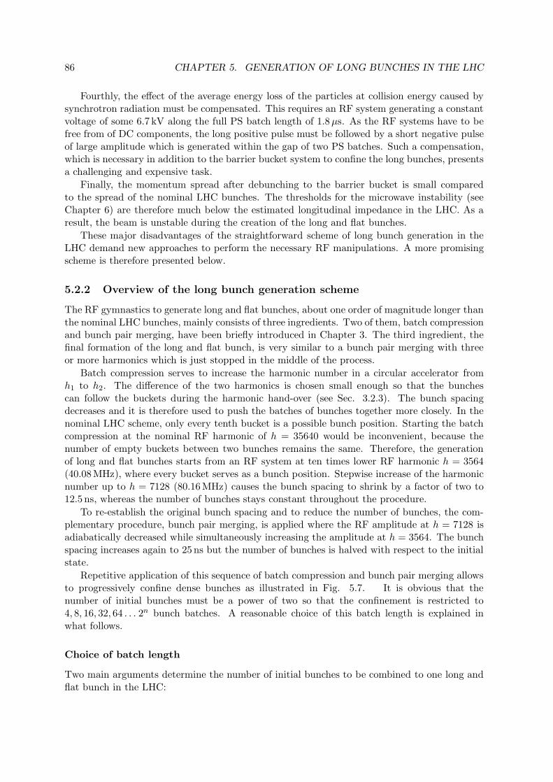
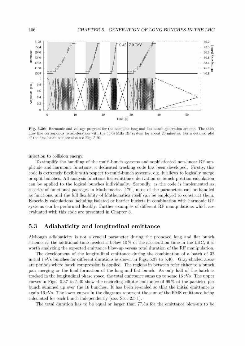
energy scaling of all particles. For the same reason, only particles within half of the batchhave been taken into account as the second half of the batch is symmetric. The complete timeoptimized harmonic and RF amplitude program used for tracking is shown in Fig. 5.36. Theacceleration in the LHC (represented by the dark gray line) will last some 20 minutes, which ismore than an order of magnitude longer than the time needed for the generation of long andflat bunches. Virtually no longitudinal emittance blow-up is expected during acceleration from


0 10 20 30 40 50Time @sD

3564

4158

4752

5346

5940

6534

7128

0

0.2

0.4

0.6

0.8

1

Am

plitu

[email protected]

Har

mon

ic

40.1

46.8

53.4

60.1

66.8

73.5

80.2

RF

freq

uenc

[email protected] 7.0 TeV

Fig. 5.36: Harmonic and voltage program for the complete long and flat bunch generation scheme. The thickgray line corresponds to acceleration with the 40.08 MHz RF system for about 20 minutes. For a detailed plotof the first batch compression see Fig. 5.20.

injection to collision energy.To simplify the handling of the multi-bunch systems and sophisticated non-linear RF am-

plitude and harmonic functions, a dedicated tracking code has been developed. Firstly, thiscode is extremely flexible with respect to multi-bunch systems, e.g. it allows to logically mergeor split bunches. All analysis functions like emittance derivation or bunch position calculationcan be applied to the logical bunches individually. Secondly, as the code is implemented asa series of functional packages in Mathematica [179], most of the parameters can be handledas functions, and the full flexibility of Mathematica itself can be employed to construct them.Especially calculations including isolated or barrier buckets in combination with harmonic RFsystems can be performed flexibly. Further examples of different RF manipulations which areevaluated with this code are presented in Chapter 3.

5.3 Adiabaticity and longitudinal emittance

Although adiabaticity is not a crucial parameter during the proposed long and flat bunchscheme, as the additional time needed is below 10% of the acceleration time in the LHC, it isworth analyzing the expected emittance blow-up versus total duration of the RF manipulation.

The development of the longitudinal emittance during the combination of a batch of 32initial 1 eVs bunches for different durations is shown in Figs. 5.37 to 5.40. Gray shaded areasare periods where batch compression is applied. The regions in between refer either to a bunchpair merging or the final formation of the long and flat bunch. As only half of the batch istracked in the longitudinal phase space, the total emittance sums up to some 16 eVs. The uppercurves in Figs. 5.37 to 5.40 show the encircling elliptic emittance of 99% of the particles perbunch summed up over the 16 bunches. It has been re-scaled so that the initial emittance isagain 16 eVs. The lower curves in the diagrams represent the sum of the RMS emittance beingcalculated for each bunch independently (see. Sec. 2.5.1).

The total duration has to be equal or larger than 77.5 s for the emittance blow-up to be

5.3. ADIABATICITY AND LONGITUDINAL EMITTANCE 107

0 20 40 60Time @sD0

5

10

15

20

25

30

35

Ú¶ l@eVsD

450 GeV 7 TeV

Fig. 5.37: Development of the elliptic (continuous)emittance containing 99 % of the particles and theRMS emittance (dashed) during the combination ofbatches of 32 bunches. The shaded areas indicate theregions of batch compression.

0 10 20 30Time @sD0

5

10

15

20

25

30

35

Ú¶ l@eVsD

450 GeV 7 TeV

Fig. 5.38: Same representation as Fig. 5.37 buttwice faster. An increased blow-up of the effectiveemittance becomes visible.

0 5 10 15 20 25Time @sD0

5

10

15

20

25

30

35

Ú¶ l@eVsD

450 GeV 7 TeV

Fig. 5.39: Same representation as Fig. 5.37 butthree times faster. The increased emittance growth issignificantly stronger than in the figures above. Dur-ing the last batch compression, particles get lost fromtheir buckets.

0 5 10 15Time @sD0

5

10

15

20

25

30

35Ú¶ l@eV

sD

450 GeV 7 TeV

Fig. 5.40: Same representation as Fig. 5.37 but fourtimes faster. Already during the second batch com-pression, particles get lost from their buckets whichvirtually leads to an exponential growth of the ellipticemittance because the particle distribution becomesnon-elliptic.

negligible and the process quasi-adiabatic. It is worth mentioning that the apparent emittancegrowth at the end of the final long bunch formation comes from artifacts of the calculationmethod. As only half of the batch is taken into account for the tracking, the batch is virtuallymerged with empty bunches. This leads to an artificial blow-up of the RMS emittance by afactor of two whereas the effect on the elliptic emittance is even more severe because the finalbunches have a non-elliptic longitudinal distribution.

In Fig. 5.38, where the sequence is executed in less than 39 s, first signs of emittance dilutionduring the RF manipulations become visible. The situation gets clearly worse when the totalduration is reduced to 25.8 s (Fig. 5.39). During the last batch compression at 7TeV particlesstart to escape and are lost. In the last case (Fig. 5.40) the result becomes even useless.Particles lost from the buckets cause an enormous emittance dilution, where the bunches arevirtually distributed all along the circumference of the LHC and finally lost.

Therefore a total time duration of 77.5 s seems adequate. The first 52.4 s of this durationare spent on the flat-bottom at 450GeV, while the remaining time is spent on the last batch


compression and bunch merging at 7TeV. This additional time needed to prepare the beamhas a negligible effect on the integrated luminosity.

5.4 Summary

After the detailed analysis of the RF manipulations necessary for the combination of 16 or 32nearly nominal bunches to a long and flat bunch, the expected performance with respect to thelongitudinal emittance is summarized for the 16 bunch scheme in Tab. 5.6.

RF parameters Emit., εl εl/ε0SPS ejection, 450GeV 8MV at 200MHz (SPS) 0.8 eVsBunch rotation and LHC injection 3MV at 40MHz (LHC) 1.0 eVs 25%Blow-up by 400.8MHz RF system 3MV at 40MHz 1.1 eVs 10%Batch compression to two bunches 2× 1.5MV at 40 . . . 80MHz 12.3 eVs 40%Acceleration to flat-top, 7TeV 3MV at 40MHz 12.9 eVs 5%Final formation of the long bunch 2× 1.5MV at 40 . . . 80MHz 28.5 eVs 10%Collision mode with long bunches 0.8/0.8/0.4MV at 40/80/120MHz 28.5 eVs

Tab. 5.6: Emittance development during the long and flat bunch generation scheme for the LHC (16⊗b⊕2⊗e).The last column εl/ε0 presents the relative blow-up of the effective longitudinal emittance estimated for themanipulation concerned. The necessity of an additional 400.8 MHz RF system causing about 10 % emittanceblow-up is due to preservation of Landau damping which is analyzed in Chapter 6.

In case of combining 32 bunches, the emittance growth is expected to be slightly larger asan additional batch compression and bunch pair merging is inserted to the RF gymnastics: thefinal emittance can be estimated to be around 2 · 28.5 eVs ' 57 eVs. The RF amplitudes inTab. 5.6 must be multiplied by a factor of four. The bunch rotation in the SPS to lengthen thebunches before extraction is not required for the combination of 32 bunches, as the RF voltage issufficient to allow a matched bunch to bucket transfer. The batch combination scheme analyzedin this chapter has several advantages compared to a superbunch scheme with barrier buckets:

Although the RF manipulations are sophisticated, RF amplitudes at no more than twoharmonics have to act on the beam simultaneously. The whole scheme can be performed withtwo or preferably three tunable RF systems in the frequency range of 40.08 to 80.16MHzdelivering about 1.5MV (16 initial bunches) or 6MV (32 initial bunches). As the LHC will befilled once or twice per day, a large tuning speed is not required, and it is thus reasonable topropose the use of vacuum cavities with high quality factor tuned by a mechanically movinggap for the large frequency variation. The PS is equipped with RF cavities at 40MHz [180, 181]and 80MHz [182] which make use of a special pneumatic gap switch operated in the ultra highvacuum of the beam pipe physically closing the accelerating gap. These cavities are operatedvery reliably and could serve as a starting point for the design of the cavities needed in the LHC.The large tuning range combined with a mechanical tuning element excludes the constructionof superconducting RF cavities.

Furthermore, the two basic ingredients for the batch combination RF manipulation, batchcompression and bunch pair merging are well-proven to work with a reasonable performance.Finally, the proposed scheme is fast in the sense that it can be performed adiabatically withinless than a few minutes. A decrease of the integrated luminosity due to the long-winded RFgymnastics is thus not expected.

5.4. SUMMARY 109

The scheme has been optimized neglecting collective beam effects like instabilities before,during or after the batch combination scheme. This important issue is addressed in the subse-quent chapter.

Chapter 6

Collective Effects and Beam Loading

In Chapter 4 the optimum luminosity conditions are calculated under the assumption thatno other collective effects than beam-beam interactions limit the longitudinal performance ofthe LHC. Also the optimization of the RF manipulations to create the long and flat bunchesis presented with main focus on single particle dynamics. Therefore, the following chapteraddresses two major longitudinal effects provoked by high intensity bunches: collective beaminstabilities and beam loading.

During storage and collision of the final long and flat bunches, the region of homogeneous linedensity is considered as a coasting beam, and consequently the Keil-Schnell criterion is derivedfrom first principles and applied to the expected long bunch parameters in the first part of thischapter. Secondly, criteria for bunched beams are introduced to estimate the beam stabilityduring the injection plateau and during acceleration of the dense bunches by the 40.08MHzRF system. Counter-measures, like the increase of the synchrotron frequency spread, are basicingredients to improve longitudinal stability being discussed thereafter. Finally, the influenceof steady-state and transient beam loading is analyzed to ensure that the new RF system couldbe controlled similarly as the superconducting 400.8MHz cavities.

6.1 Vlasov equation and Keil-Schnell criterion

A simple estimate for the longitudinal stability of a particle beam of given intensity and a welldefined momentum distribution is the so-called Keil-Schnell criterion. It has been originallydeveloped from the stability of intense coasting proton beams in the Intersecting Storage Rings(ISR) at CERN [183, 184, 185]. However, if the growth rate of the longitudinal instability islarge compared to the synchrotron frequency, the synchrotron motion of particles in a bunchedbeam can be considered as frozen on the time scale of the instability. The criterion derived inthe following section may be applied to a bunched beam as a first guess in such cases.

6.1.1 Vlasov equation and dispersion relation

The longitudinal phase space density in its most general form can be expressed by the distri-bution function g = g(θ,∆E/ω). The two independent variables are chosen as a canonicallyconjugated pair (see Sec. 2.2.2). According to Liouville’s theorem each infinitesimal longitudi-nal density fraction described by g can move in the phase space, but the total time derivative

111

112 CHAPTER 6. COLLECTIVE EFFECTS AND BEAM LOADING

of the distribution function stays constant:

d

dtg

(θ,

∆Eω

)= 0 .

Expanding the total derivatives leads to the general equation of motion

∂g(θ,∆E/ω)∂θ

θ +∂g(θ,∆E/ω)∂(∆E/ω)

˙(∆Eω

)+∂g(θ,∆E/ω)

∂t= 0 , (6.1)

which is also called Vlasov equation. The dotted variables represent total time derivatives. Asthe revolution frequencies of the individual particles ω in a high energy beam are close to theaverage revolution frequency of the beam so that ω ' ω0, the Vlasov equation reduces to [186]

∂f(θ,E)∂θ

θ +∂f(θ,E)∂E

E +∂f(θ,E)

∂t= 0 , (6.2)

where f = f(θ,E) is the adapted longitudinal distribution function.To drive the longitudinal instability, a perturbation voltage U1 at an arbitrary frequency ω1

is introduced according to U(t) = U1 exp(−iω1t) and an individual particle gains or looses acertain amount of energy per turn given by (see Eqs. 2.2 and 2.6)

∆E =eωU1

2πei(nθ−ω1t) ' eω0U1

2πei(nθ−ω1t) , (6.3)

wherein n denotes the mode number of the excitation with respect to the revolution frequency.In the case of small perturbations it, can be assumed that the perturbation of the longitudinaldensity shows the same form as the excitation itself so that

f(θ,E) = f0(E) + f1(E)ei(nθ−ω1t) (6.4)

is chosen as an ansatz representing the energy distribution of the unperturbed coasting beamf0(E) with a corresponding perturbation caused by U(t).

Inserting the derivatives of Eq. (6.4) into the Vlasov equation under the assumption thatthe perturbation amplitude f1 is much smaller than f0, the unperturbed distribution can bewritten as

i(nω − ω1)f1(E)ei(nθ−ω1t) +df0(E)dE

eω0U1

2πei(nθ−ω1t) = 0 . (6.5)

Separation of the perturbation and energy integration of Eq. (6.5) gives∫f1(E) dE︸︷︷︸I1/(eω0)

ei(nθ−ω1t) = − ieω0U1

2πei(nθ−ω1t)

∫df0(E)/dEω1 − nω dE , (6.6)

where the left side is identified by the perturbing beam current. It is worth noting that thenormalization of f(θ,E) is chosen according to∫ 2π

0

∫ ∞

−∞f(θ,E) dE = N .

The integral on the right side of Eq. (6.6) can be written in a more convenient form byconsidering that

f0(E) =dω

dEf∗0 (ω) = − η

β2

ω0

Ef∗0 (ω) ,

6.1. VLASOV EQUATION AND KEIL-SCHNELL CRITERION 113

and the Vlasov equation becomes

I1ei(nθ−ω1t) =

ie2ω30η

2πEβ2U1e

i(nθ−ω1t)

∫df∗0 (ω)/dωω1 − nω dω . (6.7)

The term on the right side contains in fact the spectral component of the beam transfer functionof a coasting beam at ω1. Introducing a complex longitudinal coupling impedance between beamcurrent U1 = −Z‖I1 to feedback the beam current perturbation as an excitation, the dispersionrelation of the coasting beam reduces to [61, 187]

1 = − ie2ω3

0ηZ‖2πEβ2

∫df∗0 (ω)/dωω1 − nω dω . (6.8)

This dispersion relation is used as a starting point to derive a criterion for longitudinal beamstability.

6.1.2 Stability diagrams

For the calculation of stability diagrams and algebraic conditions for longitudinal beam stabilitythe transformation of the dispersion relation to normalized variables is convenient. The widthof one half of the half maximum frequency spread is defined by S = −ηω0∆p/p, where ∆p/p isreferred to as half momentum spread at half maximum height1. Furthermore, the normalizedfrequency deviation of beam harmonic and excitation frequency from the average harmonic ofthe revolution frequency are defined by

nω − nω0 = xnSand ω1 − nω0 = x1nS

ω1 − nω = (x1 − x)nS .

The distribution in revolution frequencies f∗0 (ω) is converted according to

F0(x) =2πSN

f∗0 (x) ,

which is then normalized properly. For energy distributions F0(x) being symmetric aroundx = 0, the normalization conditions can be written as [189]∫ ∞

−∞F0(x) dx = 1 and F0(x = ±1) =

12F0(x = 0) . (6.9)

Finally, the normalized dispersion relation Eq. (6.8) in the new variables x, x1 becomes

1 =ieI0Z‖

2πEβ2η(∆p/p)2n

∫dF0(x)/dxx− x1

dx , (6.10)

where I0 denotes the average beam current. As the longitudinal impedance Z‖ is complex ingeneral, Eq. (6.10) can be also represented in terms of a normalized impedance:

1 = (U ′ − iV ′)∫dF0(x)/dxx− x1

dx and

U ′ − iV ′ = − eI02πEβ2η(∆p/p)2

(ImZ‖/n − iReZ‖/n

). (6.11)

1Some authors define ∆p/p as full momentum spread at half height [188] which is e.g. more convenient forthe analysis of stacked beams.


This relation couples the normalized impedance U ′ − iV ′ to the normalized complex frequencyshift x1 induced by the perturbation. The regions of impedances where the beam is stable orunstable can be explored by expressing the perturbing part of the beam distribution f(θ,E) interms of this induced frequency shift x1. As this contribution is proportional to exp[i(nθ−ω1t)],its frequency can be written as nθ = nω − ω1 = nx1S so that

exp[i(nθ − ω1t)] = exp(iRex1nηω0

∆ppt

)· exp

(−Imx1nηω0

∆ppt

).

In fact, the real part of the complex frequency shift x1 leads to a frequency displacement, whilethe imaginary part of x1 defines whether the excitation is damped (Imx1 < 0 for γ > γtr)or exponentially excited (Imx1 > 0 for γ > γtr). The trajectory in the complex impedanceplane, for which the imaginary part of x1 is zero, defines the limitation of longitudinal stability.Frequency shift and growth rate are given by

∆ω1 = −ηω0∆pp

Rex1 and1τ

= −ηω0∆pp

Imx1 . (6.12)

The full stability diagram of a given distribution is generated by evaluating the parametersU ′(x1) and V ′(x1) from Eq. (6.11) for different complex normalized frequency shifts x1; prefer-ably the parameter x1 is chosen so that either its real or imaginary part is held constant. Anexample for such a stability diagram of a quartic distribution

F (x) =15a16

(1− a2x2)2 for |x| < 1a

and a =√

1− 1/√

2

is given in Fig. 6.1. The gray shaded area is the region of normalized impedances U ′ − iV ′,

-3 -2 -1 0 1 2 3V’

-1

0

1

2

3

U’

Region ofstability

0.1 0.2 0.3 0.4 0.5

-0.2 -0.6 -1.0

-1.4

-1.8

-2.2

Im8x1<

Re8x1<F0HxL

Fig. 6.1: Stability diagram of a coast-ing beam with a quartic energy distri-bution, F0(x) ∝ (1 − a2x2)2. The grayshaded area represents the region of sta-bility as Imx1 is negative (γ > γtr)and an excitation of the beam is thusdamped. The imaginary part of x1 iskept constant along the continuous lines,while the real part remains unchangedalong the dashed lines.

which are tolerable for a stable beam. To simplify the calculation of stability diagrams, the

6.1. VLASOV EQUATION AND KEIL-SCHNELL CRITERION 115

dispersion integral from Eq. (6.11) can be integrated partially for distribution functions F0(x)which vanish at x = ± ∞ so that

U ′ − iV ′ = 1/∫

dF0(x)/dxx− x1

dx = 1/∫

F0(x)(x− x1)2

dx . (6.13)

As the integral from Eq. (6.11) contains a singularity within its integration limits are furthermoresplit into real and imaginary part according to∫

dF0(x)/dxx− x1

dx = PV∫dF0(x)/dxx− x1

dx+ sign (Imx1) iπ ∂F0(x)∂x

∣∣∣∣x=x1

(6.14)

so that a numerical computation of the stability diagrams can be performed straightforward.The principal value is defined according to

PV∫ ∞

−∞

dF0(x)/dxx− x1

dx = limε→0

[∫ x1−ε

−∞

dF0(x)/dxx− x1

dx+∫ ∞

x1+ε

dF0(x)/dxx− x1

dx

].

6.1.3 Keil-Schnell criterion

Although the explicit form of the region of beam stability is different for each distributionfunction F0(x), it is essentially centered around the origin of the stability diagram for reasonabledistributions. The stability limitation being defined by Imx1 = 0, as shown for a quarticdistribution in Fig. 6.1, is illustrated for different functions F0(x) in Fig. 6.2 [189, 190, 191].A common, stable region which is shared by most of the momentum distribution functions is

-2 -1 0 1 2V’

-0.5

0

0.5

1

1.5

2

2.5

3

U’

Gaussian

Quartic

Parabolic

Keil-Schnell

Fig. 6.2: Stability limitation for differ-ent momentum distributions in the com-plex impedance plane. The stable regionof a Gaussian beam (dotted) is signifi-cantly larger than that of a beam withquartic distribution (continuous). Theparabolic distribution shows the small-est area of stability. The gray shadedcircle illustrates the stability assumptionfor the Keil-Schnell criterion.

represented by a simple circle (gray shaded area), whose radius can be described by F · 2/π,where F is a from factor of the order of unity and the circle in Fig. 6.2 has a radius of 2/π. Itis important to point out that the tails of the momentum distribution F0(x) have a significant


influence on the longitudinal beam stability. The stability region shrinks for distributionswithout tails like parabolic or elliptic compared to Gaussian or quartic beams.

By replacing the inverse of the dispersion integral in Eq. (6.11) by the circular approximationleads to a stability limitation for the absolute tolerable impedance, namely [192]∣∣∣∣Z‖

n

∣∣∣∣ ≤ F 4Eβ2|η|(∆p/p)2eI0

. (6.15)

Originally published to estimate the beam stability in the ISR [188], this criterion has beenproven to be very useful and is therefore known as Keil-Schnell criterion. In fact, the stabilitylimitation depends inversely on the total beam current, and it is proportional to the square of themomentum spread. Beams with a sharp momentum spread are therefore prone to longitudinalinstabilities.

Although the Keil-Schnell criterion has been derived for coasting beams only, its range ofvalidity can be extended by considering the stability criterion as a local condition applied to alocal fraction of the beam. If the growth rate of the instability (see Eq. 6.12) is much fasterthan the synchrotron motion, the external RF forces can be neglected and, as a first estimation,it may even be applied to bunched beams [193, 194, 195]. Consequently, the average beamcurrent I0 as well as the momentum spread ∆p/p have to be exchanged by their local values.This effect of a very fast growing bunch excitation is referred to as microwave instability as itspresence is accompanied by a bunch signal in the microwave range above several hundred MHz,well above the bunch frequency [196]. It is worth noting that the term microwave instability isalso used for several other instabilities having a high frequency bunch signal as its characteristicsignature.

6.1.4 Stability of the LHC beam during long and flat bunch collision

By definition, the long and flat bunches or superbunches in collision mode have a region ofnearly homogeneous line density with a length of at least some 10ns. This coasting beamsection can be treated as such if the inverse instability growth rate is faster than the drift timeof the particles between the two bunch ends and if the coasting beam section is excited atfrequencies well above 100MHz.

The effective threshold impedance according to the Keil-Schnell criterion for coasting beamsfrom Eq. (6.15) is illustrated in Fig. 6.3 for the long and flat bunches and compared to the maxi-mum longitudinal density of nominal and low emittance nominal bunches. The total longitudinalimpedance in an accelerator is evaluated by summing up all contributing elements installed inthe vacuum chamber, each of which is analyzed by means electromagnetic field calculations forits specific geometry. A complete table of impedance estimations for the contributing elementsis given in [197] and the total longitudinal impedance is estimated to |Z‖/n| = 0.076Ω.

Compared to the instability thresholds in Fig. 6.3, even the case of a superbunch with alongitudinal density at the beam-beam limit corresponding to a local current of some 131Ais stable with respect to the Keil-Schnell criterion. The limit is found to be around |Z‖/n| =0.165Ω. It is worth noting that the local density of the nominal bunches as well as those of thelow emittance nominal bunch has more than one order of magnitude of safety margin.

6.2 Landau damping

The so-called Landau damping is an effect of apparent natural damping which occurs whenan ensemble of oscillators with slightly different resonant frequencies is excited by a coherent

6.2. LANDAU DAMPING 117

0 0.2 0.4 0.6 0.8 1 1.2 1.4Dpp @10-4D0

0.2

0.4

0.6

0.8

1

1.2

1.4

ÈZ þnÈ@WD M

inim

umsu

perb

unch

Smal

lem

ittan

ce:1

eVs

Nom

inal

:2.5

eVsI0 = 26.5 A

42.3 A

131 AFig. 6.3: The graphs represent the Keil-Schnell limit of the tolerable, effective lon-gitudinal broad band impedance to pre-serve the stability of the coasting beamsection of a long and flat bunch or a su-perbunch at collision energy. It is givenfor a local beam current of 26.5 (dot-ted), 42.3 (dashed) and 131 A (continu-ous) which corresponds to the local densityof the nominal, the low emittance nomi-nal (see Tab. 5.2 and the minimum emit-tance long or superbunch (see Tabs. 4.5and 4.6). The momentum spread as halfwidth half maximum of the correspondingparabolic distribution is indicated by thevertical lines.

signal [198]. In fact, a particle bunch treated in the longitudinal phase space plane is such asystem: the individual particles oscillate around the center of gravity of the bunch while theirindividual oscillation frequencies vary with their maximum phase deviation from the center.This distribution of frequencies is calculated in Sec. 2.2.6 and in App. D. As becomes clearfrom Fig. 6.4, the beam behaviour of the individual particles depends on the RF configuration,even though the bunch projections might be identical. Therefore, only a small fraction ofthe particles in a bunch with a large synchrotron frequency spread (Fig. 6.4) are excited byan harmonic excitation, whereas a bunch with a small synchrotron frequency spread may beexcited easily as a whole.

Landau damping of the longitudinal dipole motion can be investigated by calculating theaverage bunch motion from the subset of individual particles within the bunch [199]. Thesynchrotron oscillation of a single particle driven by a harmonic excitation is described by

φ+ ω2sφ = e−iωt , (6.16)

where φ denotes the phase deviation from the bucket center and ω is the frequency of the drivingterm. The driving amplitude is arbitrarily normalized to unity. The single particle solution ofEq. (6.16) proportional to the driving term can be written as

φ(t) =φ

ω2s − ω2

e−iωt .

The distribution of resonance frequencies of N particles in the bunch is represented by thefunction G(ω) = 1/N dN/dωs and is normalized so that the integral over all frequencies givesunity. It is worth mentioning that this frequency distribution is also symmetric with respect tonegative frequencies: G(ωs) = G(−ωs). In fact, G(ωs) dωs is the fraction of individual oscillatorshaving a resonance frequency between ωs and ωs + dωs.


-Π 0 ΠΦ @radD

-2

-1

0

1

2

DE

@GeVD400.8 MHz,16 MV

-Π 0 ΠΦ @radD

-2

-1

0

1

2

DE

@GeVD

400.8 MHz,16 MV

-Π 0 ΠΦ @radD

-2

-1

0

1

2

DE

@GeVD

40.08 MHz,160 MV

Fig. 6.4: Tracking of particles on a net to illustrate a stationary bunch during one period of the linear synchrotronfrequency. The left phase space shows the initial bunch. After one synchrotron period in a 400.8 MHz bucketwith an RF voltage of 16 MHz (center) it becomes obvious that the synchrotron frequency in the outer regionsof the bunch is reduced. The right phase space shows the same bunch in a matched 40.08 MHz bucket. Theseparatrix is not visible as it is far away from the bunch. The whole bunch can be considered to be within thelinear region of the bucket so that no dispersion is visible. It is important to point out that the RF amplitudeof 160 MV has only been chosen as an example to obtain matched bunches under the same conditions as for the400.8 MHz system.

The average dipole motion of the whole ensemble of oscillators is expressed by

<φ(ω)>=[∫ ∞

−∞

G(ωs)ω2s − ω2

dωs

]e−iωt , (6.17)

where the integration over negative frequencies is included for convenience. Part of the integrandcan be expanded according to [200, 201]

1ω2s − ω2

=12ω

(1

ωs − ω −1

ωs + ω

)

so that the average bunch motion Eq. (6.17) reduces to

<φ(ω)>=12ω

[∫ ∞

−∞

G(ωs)ωs − ω dωs −

∫ ∞

−∞

G(ωs)ωs + ω

dωs

]e−iωt =

[1ω

∫ ∞

−∞

G(ωs)ωs − ω dωs

]e−iωt .

(6.18)The singularity of the integrand at ω = ωs leads to a complex solution of the integral in Eq. 6.18which can be split into real and imaginary part according to

<φ(ω)>=1ω

[PV

∫ ∞

−∞

G(ωs)ωs − ω ± iπG(ω)

]e−iωt , (6.19)

where PV is again the principal value excluding the singularity. From the velocity variation ofthe bunch center, namely

d

dt<φ(ω)>= −iω <φ(ω)>=

[πG(ω)− iPV

∫ ∞

−∞

G(ωs)ωs − ω dωs

]e−iωt , (6.20)

it becomes clear that the first term is in phase with the initially applied driving term (seeEq. 6.17), whereas the second term always has a phase deviation of π/2. Therefore, the inphase contribution absorbs energy from the driving force and leads to a virtual damping of

6.3. LONGITUDINAL BUNCHED BEAM STABILITY IN THE LHC 119

the average dipole motion of the bunch. However, only the average motion of the ensembleof oscillating particles is damped and individual particles may be excited enormously. It isinteresting to note that the damping term is proportional to the value of the density functionat the excitation frequency and that it vanishes once the excitation frequency is outside ofthe synchrotron frequency spread so that G(ω) = 0. The preservation of Landau damping istherefore mandatory to prevent particle beams from exciting themselves due to self-inducedperturbations. Comparing Eq. (6.20) with the dispersion integral Eq. (6.8) for coasting beamsreveals that coasting beam stability is based on Landau damping.

6.3 Longitudinal bunched beam stability in the LHC

There are two different classes of longitudinal bunched beam instabilities. On the one hand,single bunch instabilities are based on the excitation of longitudinal oscillations of the particledistribution within the bunch. On the other hand, multi-bunch instabilities arise because of acoupling between different bunches within a batch so that different bunches oscillate in phasewith respect to each other. The order of the single bunch oscillation mode is identified by themode number m whereas the mode along the bunch train of M equal bunches in the acceleratoris denoted as n = 1 . . .M [202]. The phase advance between two bunches is described by2π n/M . Considering that the bunch shape oscillation is in fact a rotation of the perturbedlongitudinal distribution with the synchrotron frequency and that the coupled bunches circulatewith the revolution frequency, the excitation frequency for all possible modes can be written as

ω = hω0 ±mωs ± nω0 = ωRF ±mωs ± nω0 . (6.21)

The following analysis of bunched beam stability is limited to equidistant bunches held by singleharmonic RF system and is not applicable to the bunches during RF gymnastics, where moreRF systems act on the bunches simultaneously.

6.3.1 Bunch shape oscillations

The first six single bunch modes are illustrated in Fig. 6.5. One can observe that the number ofnodes in the line density plots corresponds to the mode number. The oscillation frequencies ofthe modes are directly given by ω = mωs, which becomes obvious considering that a distorteddistribution of the mode m just needs to be rotated by 2π/m to reproduce itself.

6.3.2 Coupled bunch oscillation modes

The second kind of possible oscillations of a bunch train in a circular accelerator are coupledbunch modes. These modes are mostly excited by resonators with a high quality factor, andtherefore a narrow bandwidth, which are coupled to the beam. The long time constant of thefield decay in the resonators bridges the time distance between two or even more bunches. Infact, the cavity is excited by a bunch passing through and the excited electromagnetic fieldsact back on the subsequent bunch train. The number of possible oscillation modes is identicalto the number of bunches in the accelerator. An illustration of the four longitudinal coupledbunch modes of a bunch train consisting of four bunches is given in Fig. 6.6. For the modenumber n the phase position of the M bunches is calculated according to [203]

∆φi(t) = ∆φ0 cos(ωt− 2π

n

Mi), (6.22)


m = 0 m = 1 m = 2 m = 3 m = 4 m = 5

Fig. 6.5: Illustration of the single bunch oscillation modes m = 0 . . . 5. Whereas the upper row shows the bunchoutline for two different phases of the oscillation, the center row presents the longitudinal distribution assumingparabolic bunches. The resulting line density is sketched in the bottom row. The zeroth mode just results in astationary parabolic bunch.

where i is the number of the bunch and ∆φ0 its maximum phase excursion. The Landaudamping time constant of single bunch higher order oscillation modes as well as coupled bunchmodes can be larger or smaller as their inverse growth rate resulting in stable, damped orexponentially growing oscillations.

6.3.3 Narrow band resonator impedances

The complex synchrotron tune shift for bunched beams and finally a criterion for the longitu-dinal stability of bunched beam can be derived similarly to the calculation of the Keil-Schnellcriterion for coasting beams as shown in Sec. 6.1. However, adding the synchrotron motion in-troduces considerable complexity to the calculation so that only the basic ideas shall be given inthis report. The full derivations and the underlying theory can be found in [204, 205, 206, 207].The procedure to derive longitudinal bunched beam instabilities is summarized as follows [208]:

As shown for the case of a coasting beam, a reasonable unperturbed beam distribution ischosen firstly and a small perturbation is added to it. Secondly, the local density f(τ,E, z) isderived and inserted into the Vlasov equation, wherein the external force due to the synchrotronmotion is also taken into account. The ansatz for the perturbed local density function, namely

f(τ,∆E, z) = f0(τ,∆E) + f1(τ,∆E, z) , (6.23)

is chosen in such a way that only the perturbed part depends on the longitudinal position z.The unperturbed part is not influenced by the excitation caused by preceding beam particles,however is contributes to the excitation of subsequent beam. It is worth noting that the coordi-nate system can be defined so that the unperturbed synchrotron motion of the single particles istransformed to circles in a normalized longitudinal phase space. This allows an easy separation


Fig. 6.6: Illustration of the possible coupled bunch modes of four bunches in a circular accelerator. Besides ofa phase difference of π, the first and the third mode are identical in this case.

of the radial modes (illustrated in Fig. 6.5), and the local density can be written as

f0(r) dτ dE = Ng0(r)r dr dφ (6.24)

where g0(r) is the radial distribution normalized according to∫ 2π

0

∫ ∞

0g0(r)r dr dφ = 1 . (6.25)

It should be pointed out that the radius is defined in time units [r] = [time] = s. Finallyone ends up with a dispersion relation similar to the dispersion relation of coasting beams butincluding a general longitudinal force. This force must be expressed in such a way that theinfluence of preceding on subsequent particles passing through the accelerator is incorporated.

The dispersion relation for a perturbation excited by a narrow band cavity with the shuntimpedance Rs at the resonance frequency ωr can be written as [207]

1 = −ie2NRsmMηω2

0

2πEβ2ωsωrD(ατsep)

∫ ∞

0

dg0(r)dr

J2m(ωrr)

ω −mωs(r) dr , (6.26)

where Jm denotes the m-th Bessel function of the first kind. The parameter α represents theinverse filling time ωr/(2Q) of the cavity and the function

D(ατsep) = −i2ατsep∞∑k=0

e2πikn/M−k(α−iω)τsep sin(kωrτsep)

describes the coupling between the bunches and the resonator, taking the bunch spacing fielddecay within the bunch spacing into account [202]. In case of a small relative synchrotronfrequency spread [ωs(r)− ωs]/ωs 1, the complex synchrotron frequency shift is expressed by

∆ω = ω −mωs = ie2NMRsηω

20

8π2Eβ2ωsτD(ατsep)Fm(2ωr τ) (6.27)


withFm(2ωr τ) = −4πmτ

ωr

∫ ∞

0

dg0(r)dr

J2m(ωrr) dr .

The form factor Fm is plotted for a parabolic (left) and quartic (right) distribution in Fig. 6.7.The bunches have a total length of 2τ . It is worth noting that Eq. (6.27) is consistent with the

0 5 10 15 20ΩrH ΒcL × total bunch length

0.2

0.4

0.6

0.8

1

1.2

F

m = 1

2

34

5

0 5 10 15 20ΩrH ΒcL × total bunch length

0.2

0.4

0.6

0.8

1

1.2

F

m = 1

2

34

5

Fig. 6.7: Form factor F (2ωr τ ) for parabolic (left) and quartic (right) radial distribution function g0(r).

synchrotron tune shift given in [202].In analogy to the calculations for coasting beam stability a simple stability criterion based

on circles in the complex stability diagram can be given from the analysis of the dispersionintegral in Eq. (6.26). Landau damping is preserved as long as [202]

1τ<

√m

4∆ω , (6.28)

and the excited mode of coupled bunch oscillations remains stable. This means for dipoleoscillations that the tune spread in synchrotron frequency should be four times wider than thetune shift due to the narrow band resonance.

For a first estimation of longitudinal stability considering the most sensitive mode, thecoupling function D(ατsep) can be replaced by its maximum value as illustrated in Fig. 6.8.Clearly, the coupling function becomes small for driving impedances having small field decay

0.01 0.05 0.1 0.5 1 5 10ΑΤsep

0

0.2

0.4

0.6

0.8

1

ÈDÈ max broadband

narrowband

Fig. 6.8: Maximum of the coupling function versusατsep = πωr/(QMω0). The number of equally dis-tributed bunches is defined by M .

durations compared to the bunch frequency. Consequently, a preceding bunch has almost no


influence on the subsequent particles. However, for resonators with a large quality factor, asit is mostly the case for higher order mode resonances of RF cavities or parasitic resonance inmetallic objects within the accelerator like pumping slots, the coupling function D(ατsep) canbe approximated to unity.

Following the stability criterion imposed by Landau damping from Eq. (6.28), the maximumtolerable narrow band impedance is derived considering that the growth rate is defined as theinverse imaginary frequency shift (see Sec. 6.1.2). Landau damping is thus preserved as longas the shunt impedance of the driving resonance fulfills the relation

Rs .√mU0 cos φ0ω0

2I0τh

M

∆ωsωs

/[D

(πωrQMω0

)F (2ωr τ)

], (6.29)

where I = NMeω0/(2π) denotes the total beam current, and where M equidistant bunches areassumed. The total bunch length is given by 2βcτ . The azimuthal dipole mode m = 1 is mostprone to a coupled bunch instability due to a narrow band excitation as the tolerable thresholdimpedance increases proportionally to

√m, and also the maximum height of the bunch form

factor Fm(2ωr τ) as shown in Fig. 6.7 decreases with the mode number.

6.3.4 Broad band impedance

In the preceding section, the narrow band resistive impedance driving the coupled bunch insta-bility is assumed to be the only impedance present in the accelerator. However, in real machinesa so-called broad band impedance, which is in fact the contribution of all components, like bel-lows, monitors or kicker magnets seen by the beam, is modeled as broad band resonance. Thisbroad band resonator directly has a negligible effect on the coupled bunch instabilities, as thefields in this virtual resonator decay much faster than the bunch spacing (see Fig. 6.8). How-ever, it contributes to the synchrotron tune shifts, displacing them in such a way that Landaudamping can be lost for coupled bunch modes which would be well damped according to Eq.(6.28) neglecting the broad band impedance.

Following the analysis in [205, 206], the absolute tune shift due to the longitudinal broadband impedance can be written as

∆ω = −i π3I03τ3ω3

0U0 cos φ0

1Mh

mωsm+ 1

∞∑p=−∞

Z(p)p

hmm(p)

/ ∞∑p=−∞

hmm(p)

︸︷︷︸(Z‖/n)eff

, (6.30)

where the coefficients hmm(p) denote the relative spectral power of the bunches at the frequencypω0. It is convenient to define an effective longitudinal impedance (Z‖/n)eff including thespectral distribution [209]. Landau damping for the m-th mode is preserved as long as

1τ

= −Im∆ω < 12

m

m+ 1∆ωs .

It is worth noting that longitudinal coupled bunch modes are driven by the imaginary part ofthe effective impedance only. The threshold impedance can be derived by inserting Eq. (6.30)into the criterion for Landau damping, namely2(

ImZ‖n

)eff

. 32π2

Mh3U0 cos φ0

I0

∆ωsωs

τ3ω30 . (6.31)

2A different derivation of the criterion finally ends up with the same result as Eq. (6.31) for π ' 3 [210].


It should be pointed out that the instability threshold criteria for longitudinal narrow as wellas broad band impedances are, due to the formulation of the Landau damping criterion, pro-portional to the synchrotron frequency spread of the bunch. An artificial increase of the spreadnormally results in improved bunched beam stability.

6.3.5 Stability of the LHC beam during long and flat bunch scheme

The longitudinal stability of the nominal LHC beam during injection flat-bottom, accelerationand collision mode held by the superconducting RF system operated at 400.8MHz has beenanalyzed in detail by several authors [209, 211, 212, 213, 214, 215, 216]. Basically, the stabilitycriteria introduced above have been applied to the relevant beam parameters. However, duringthe RF manipulation at injection and collision energy, multiple RF harmonics act on the beamsimultaneously and the criteria are not strictly valid anymore. They may only give a firstestimation of stability as the bunches are held by a single harmonic RF in between the sub-steps of the batch combination scheme.

The longitudinal stability during the long and flat bunch generation scheme presented inChapter 5, as well as during acceleration of partly combined bunches with a 40.08MHz RFsystem, is estimated in this section.

The longitudinal beam parameters during acceleration in the LHC are derived on the basisof the realistic magnetic cycle [217] of the LHC dipole magnets, which is assumed to remainunchanged with respect to the nominal scheme. The magnetic dipole induction correspondingto the particle energy and its first derivative are sketched in Fig. 6.9. The ramp rate is varied

0 400 800 1200 1600Acceleration time @sD0

2

4

6

8

B@TD

0

2

4

6

8

10

dBdt@mT

sD

Fig. 6.9: Magnetic cycle of the LHC dipolemagnets during acceleration (continuous). Thefirst derivative is shown as a dashed line.

smoothly at the beginning as well as at the end of the acceleration. The maximum ramp rateof 7.3mT/s is limited by the voltage capabilities of the main power converters. It is importantto point out that the average energy gain of the particles during acceleration does not exceed485 keV/turn.

Fig. 6.10 shows the longitudinal emittance development during the cycle according toTab. 5.6 as well as the available bucket area. The bucket area during acceleration is pre-sented for a constant RF amplitude of 3MV throughout the cycle. In fact, 2 · 1.5MV would beavailable in a scheme where 16 bunches are combined to one long and flat bunch. At the injec-tion flat-bottom, a linear increase from about 1 eVs to the emittance of the combined bunchesof 12.9 eVs is assumed for simplicity. During this linear increase, the time scale in Fig. 6.10has no validity, as the combination scheme is performed within one minute, too fast to be vis-ible in the plot. Furthermore, the longitudinal emittance does not increase linearly due to there-combination of bunches but rather stepwise with each bunch pair merging.



20

40

60

80

100

¶,A

@eVsD450 GeV 7 TeV

Bucket area, A

Bunch emittance,¶

Fig. 6.10: Bucket area (upper curve) andbunch emittance (lower curve) during the LHCacceleration cycle including the combinationscheme of 16 initial bunches to a long and flatbunch. The area shaded in dark gray representspossible bucket areas at 40.08 MHz (h = 3564)for an RF amplitude between 1.5 and 3MV.The light gray shaded area below shows thebucket area for 1.5 MV RF voltage in the fre-quency range from 40.08 to 80.16 MHz thatmeans during the combination RF gymnastics(see also Fig. 5.10).

The qualitative behaviour of bucket area and beam emittance of the second long and flatbunch option combining 32 bunches is equivalent to the graphs shown in Fig. 6.10. The quadru-pled RF voltage of 2·6MV results in twice the bucket area, and the longitudinal beam emittanceis assumed to grow to some 26 eVs; twice the bunch emittance of the 16 bunch scheme due tothe further bunch merging at flat-bottom. At collision energy one also finally ends up with twicethe bunch emittance. It is however worth mentioning that the filling factor, the ratio betweenbunch emittance and bucket area, remains constant for the 16 and the 32 bunch combinationoption.

Tolerable narrow band impedance

For a worst-case estimation of the tolerable resonator impedances to preserve Landau dampingof coupled bunches bunch modes in the LHC, the form factors in Eq. (6.29) can be substitutedby their maximum values: according to Figs. 6.8 and 6.7 the coupling function D(πωr/[QMω0])is set to unity and the form factor F (2ωr τ) is approximated to 1.05 for the dipole mode m = 1.

Evaluating Eq. (6.29) according to these simplifications, and with respect to the set of beamparameters introduced above, results in the development of the impedance threshold during theLHC cycle as plotted in Fig. 6.11. Even though the bunch intensity was assumed to be only

0 400 800 1200 1600Acceleration time @sD0.00

0.1

0.20

0.30

0.40

Rs

@MWD

450 GeV 7 TeV450 GeV 7 TeV

Fig. 6.11: Worst case estimation of the tol-erable narrow band impedance along the LHCcycle for a constant RF amplitude of 3MV at40.08 MHz (16 bunch scheme, continuous) and4 · 3MV (32 bunch scheme, dotted). The ini-tial bunch intensity is assumed to be nominal inboth cases: 1.15 ·1011 ppb. The stability criteriacan be only applied rigorously during accelera-tion, as multiple harmonic RF systems act onthe beam otherwise.

1.15 · 1011 ppb, the minimum threshold impedance is more than an order of magnitude belowthe threshold for operation with the 400.8MHz RF system [212]. In fact, two problematicregions can be determined: firstly, during injection, when the bunches with a small emittanceare injected to the huge buckets at 40.08MHz. Secondly, when approaching the collision energy


due to the energy dependence of the threshold impedance. A potential cure for the former isproposed in Sec. 6.3.6. Analyzing the scaling of the threshold impedance indicates the mainreason for the severe stability limitations of the beam held by a 40.08MHz RF system. Forenergies well above transition, so that the phase slip factor η remains constant and for ultra-relativistic beams, it scales according to

Rs ∝ε3/2l h9/4U

1/40

E3/4∝ U0

(εlA

)2,

where εl/A denotes the bucket filling factor. Consequently the bunches are prone to becomeunstable if the buckets are sparsely filled. This is the case for the tiny bunches at injectionand at the end of the acceleration, when the bucket area increases proportional to

√E times

the area reduction factor due to the non-zero synchronous phase (see 2.2.5). Furthermore, thethreshold scales as h9/4U1/4 so that higher harmonics of the revolution frequency are preferableto hold and accelerate low longitudinal emittance bunches.

Tolerable broad band impedance

A similar analysis can be performed to estimate the threshold of the longitudinal broad bandimpedance as derived in Eq. (6.31). Fig. 6.12 shows this threshold (ImZ‖/n)eff along theacceleration cycle. The graph looks qualitatively similar to the narrow band impedance


2

4

6

8

10

HIm8Z þ<nL eff@W

D

450 GeV 7 TeV450 GeV 7 TeV

Fig. 6.12: Worst case estimation of the tol-erable broad band impedance along the LHCcycle for a constant RF amplitude of 3MV at40.08 MHz (16 bunch scheme, continuous) and4 · 3MV (32 bunch scheme, dotted). The bunchintensity is assumed to be nominal.

limitation as illustrated in Fig. 6.11. The problematic phases can again be identified duringinjection and at the end of the injection cycle. The former region during injection wouldimpose a severe limitation of (ImZ‖/n)eff ' 0.0058Ω for the nominal bunch intensity tothe tolerable broad band impedance so that bunches would certainly become unstable withoutcounter measures. As soon as the longitudinal emittance increases during the combinationprocedure, the threshold stays well above the estimated broad band impedance of 0.076Ω inthe LHC. The scaling of the threshold impedance can be written as(

ImZ‖n

)eff

∝ ε5/2l h7/4

E5/4U1/40

∝ U0

h2

(εlA

)5/2,

wherein the strong dependence on the bucket filling factor becomes apparent. Furthermore, thethreshold decreases rapidly with growing beam energy.

The reduced threshold is partly attributed to the small synchrotron frequency spread of lowemittance bunches in large RF buckets. Applying means to increase the synchrotron frequency


spread avoiding unreasonable blow-up, the longitudinal emittance improves the stability thresh-old for broad band as well as for narrow band impedances directly proportionally (see Eqs. 6.29and 6.31). This counter measure is discussed in the subsequent section.

The installation of an additional RF system to capture and hold the beam during the fillingprocedure of the LHC rings could be envisaged as a second counter measure; e.g. a capture RFsystem operated at 200.4MHz in the LHC has already been considered and designed [218] upto the construction of the required normal conducting cavities, but has been finally postponed[219, 220]. This system would be potentially available for the upgrade. Filling the two LHCrings by injecting into 200.4MHz bucket would provide stable beams until the hand-over tothe 40.08MHz RF system. The bunch combination scheme to generate long and flat bunchescould commence immediately and the sojourn time of the small emittance bunches in the largebuckets could be reduced to the order of a few seconds. This might be sufficient if the instabilitycannot grow fast enough during this period.

6.3.6 Increase of the synchrotron frequency spread

Both narrow band and broad threshold impedances for longitudinal bunched beam stability aredirectly proportional to the relative spread of the synchrotron frequencies within the bunch.In the case of bunches in stationary buckets (see Eq. 2.43), the relative synchrotron frequencyspread in the single harmonic RF system is expressed in terms of the longitudinal emittance εlas

∆ωsωs

=116

√2|η|ω2

0h3

πEβ2eU0· εl , (6.32)

where the emittance is given in units of eV ·s. In fact, decreasing the RF harmonic by one orderof magnitude from h = 35640 to 3564, as proposed for the long and flat bunch generation scheme,and decreasing the RF voltage by a factor of approximately another order of magnitude, reducesthe synchrotron frequency spread by a factor of ten. This results in an unstable beam during thegeneration of long and flat bunches. Inserting the stationary bucket area into Eq. (6.32) reducesit to ∆ωs/ωs = 1/

√π · εl/AeVs so that the spread is actually proportional to the relative filling

factor of the bucket. Consequently, the synchrotron frequency spread of bunches in 40.08MHzbuckets is lowest during the injection of the small bunches from the SPS, where the bucket areais large compared to the tiny bunch emittance in the range of 1 eVs. After the combination ofseveral of these bunches, the situation becomes less critical. Adding some higher harmonic RFamplitude is a well known technique to increase the synchrotron frequency spread of a bunch[168, 169], which shall be analyzed in what follows.

Synchrotron frequency spread including a higher harmonic RF system

For an arbitrary RF amplitude function, the synchrotron frequency of a particle oscillatingon a closed trajectory can be written in integral form according to Eq. (2.41), and analyticapproximations for a stationary as well as for an accelerating harmonic bucket are given inSec. 2.2.6 and App. D.

The influence of increasing the synchrotron frequency spread of the low emittance bunchesto the large RF buckets at 40.08MHz can be analyzed numerically. The following assumptionsfor the higher harmonic RF system have been made: firstly, the synchrotron frequency spreadof a 1 eVs bunch should be increased by at least one order of magnitude. Secondly, the higherharmonic RF systems should be compatible with the RF manipulations so that it can stay activealso during the first combination steps of the long and flat bunch generation procedure. This


implies that the increase in synchrotron frequency must be sufficient for any phase relationbetween main RF focusing. The longitudinal emittance dilution due to the additional RFsystem should be below 25% to keep the degradation of the longitudinal beam quality withinreasonable limits.

The frequency of the higher harmonic has be chosen so that it results in a significant slopevariation of the effective RF focusing along the bunch. Considering that the initial bunch lengthin the LHC is of the order of 4 ns, the use of 200.4MHz and 400.8MHz is investigated. Therelative synchrotron frequency versus single particle emittance is plotted in Figs. 6.13 and 6.14.It is interesting to note that the influence on particles with a certain emittance is compensated

0 2 4 6 8 10 12 14Single particle emittance @eVsD

-0.2

-0.1

0

0.1

0.2

-D

ΩΩ s

LHC, 40.08 MHz, 1.5 MV400.8 MHz, 0.15 MV

Fig. 6.13: Relative synchrotron frequency deviationversus single particle emittance for a combination of40.08 and 400.8 MHz RF amplitude in the LHC atinjection flat-bottom. The ensemble of continuouscurves is calculated for phase relations between thetwo RF systems, varying from 0 to π in steps ofπ/10. The dashed line shows the unperturbed relativesynchrotron frequency of the 40.08 MHz RF systemalone.

0 2 4 6 8 10 12 14Single particle emittance @eVsD

-0.2

-0.1

0

0.1

0.2

-D

ΩΩ s

LHC, 40.08 MHz, 1.5 MV200.4 MHz, 0.15 MV

Fig. 6.14: Same representation as in Fig. 6.13 butfor the combination of 40.08 and 200.4 MHz. The rel-ative spread for bunches with an emittance smallerthan 1.5 eVs is significantly reduced compared tothe higher harmonic RF system operated at twice200.4 MHz. The gray shaded area represents the nom-inal bunch emittance.

so that they oscillate with the single harmonic synchrotron frequency, unaffected by the phaseof the higher harmonic RF.

As shown in Fig. 6.13, only some 150 kV at 400.8MHz would suffice to restore a relative syn-chrotron frequency spread comparable to ∆ωs/ωs = 0.1 of the nominal LHC bunch. However,the large frequency ratio between the main and the higher harmonic system is mandatory toobtain large synchrotron frequency spreads within small bunches, independent from the phaserelationship of the two RF amplitudes (see Fig. 6.13). It is important to point out that thesuperconducting 400.8MHz RF installations cannot be employed directly as higher harmonicRF system. Due to their large shunt impedance, the beam induces too much voltage in theeight cavities to control the RF amplitude down the level of 150 kV (see Sec. 6.5).

Emittance blow-up

Following the analysis in the preceding section, the synchrotron frequency spread of smallbunches in large buckets can be increased significantly by adding some higher harmonic RFvoltage to the main bucket. However, bunches with in elliptic boundary injected to such adouble harmonic RF system are not perfectly matched anymore, resulting in emittance blow-up depending on the frequency and the amplitude of the higher harmonic system. After someinitial emittance dilution, the bunch matches itself to the perturbed trajectories of the bunch so

6.4. RF PHASE STABILITY IN LONG BUNCH COLLISION MODE 129

that virtually no further emittance increase is expected after a few periods of the synchrotronfrequency.

The emittance blow-up of a bunch held in a 40.08MHz bucket caused by some RF voltageat 400.8MHz is presented in Fig. 6.15. It can be obtained by tracking a parabolic bunch with

0 500 1000 1500 2000RF voltage at 400.8 MHz @kVD0

0.5

1

1.5

2

2.5

¶ l@eVsD

1.5 MV at 40.08 MHz

3.0 MV

Fig. 6.15: Blow-up after full dilution of aparabolic bunch injected into a double harmonicRF system 40.08/400.8 MHz, where the higherharmonic RF amplitude increases the spread ofsynchrotron frequencies within the bunch. Themain RF voltage is set to 1.5 and 3MV.

an initial elliptic contour under the influence of the two RF systems. The emittance dilutionincreases proportionally to voltage at 400.8MHz and up to some 0.5MV it remains well below25%. Under these conditions, it is therefore justified to assume an increase of the synchrotronfrequency spread by one order of magnitude for the longitudinal stabilization at the cost ofsome 25% in emittance (see Tab. 5.6).

Non-harmonic RF system

Up to now the ratio of fundamental and higher harmonic RF system has been assumed to bewhole numbered so that both contributions to the RF buckets are symmetric to the referenceenergy. Setting the higher harmonic system to a non-integer harmonic shifts the energy ofthe sub-buckets with respect to the average beam energy in the main RF buckets. In fact,the frequency offset causes a phase slippage of main and sub-bucket, leading to a continuousvariation of the local synchrotron frequency within the bunch.

However, as can be seen in Fig. 6.16, the application of such a scheme can introduceparametric resonances due to the phase slippage of the higher harmonic RF system, whichmoves in the same direction as individual particles in spheres of influence of the off-energysub-buckets.

Tracking calculations like the example above show that the development of the effectivelongitudinal emittance is very sensitive to energy offset and amplitude of the higher harmonic.During batch compression, the RF focusing of the individual bunches varies along the batchso that also the coupling between main and higher harmonic RF system changes continuously.Therefore, such a scheme cannot be applied straightforward in combination with the long andflat bunch generation scheme in the LHC.

6.4 Synchrotron frequency distribution with respect to RF

phase stability in long bunch collision mode

The synchrotron frequency distribution during storage of the final long bunches in bucket gen-erated by multiple RF harmonics is of special interest as the bunches are stored in this mode for


-Π 0 ΠΦ

-0.75

-0.50

-0.25

0

0.25

0.50

0.75

DE

@GeVD

-Π 0 ΠΦ

-0.75

-0.50

-0.25

0

0.25

0.50

0.75

DE

@GeVD-Π 0 Π

Φ

-0.75

-0.50

-0.25

0

0.25

0.50

0.75

DE

@GeVD

Fig. 6.16: Development of a 1 eVs bunch held by an RF voltage of 1.5 MV at 40.08 MHz under the influence oftwo additional higher harmonic RF systems at 400.8 MHz. The higher harmonic RF systems have an amplitudeof some 150 kV. They are operated symmetrically slightly below and above the integer harmonic. Their centerenergy is indicated by the continuous horizontal lines, and their bucket height is illustrated as gray stripes. Thegray shaded macro-particles are tracked for reference only. The dashed emittance ellipse contains 99 % of theparticles. The phase space on the left shows the initial phase space while center and right plot illustrate thebunch after 0.64 and 2.1 periods of the synchrotron frequency.

several hours. Studies in the SPS with bunches held by a double harmonic RF bucket generatedby the 200 and 800MHz have shown that the phase stability between both RF systems mustbe kept within tight tolerances if the bunches should be stretched [168].

The synchrotron frequency distribution for the final long bunches held by two, three and fourmultiples of 40.08MHz is illustrated in Fig. 6.17. The synchrotron frequencies of particles with

0 0.2 0.4 0.6 0.8 1 1.2 1.4Norm. trajectory emittance

0

0.2

0.4

0.6

0.8

1

ΩΩ s

Fig. 6.17: Relative synchrotron frequency versus single par-ticle emittance normalized to bucket area of the single har-monic bucket for the voltage ratios given in Tab. 4.3. Thedistribution for three RF harmonics is represented by thecontinuous line while dashed and dotted lines show the casefor two and four RF harmonics. The phase relation betweenthe different harmonics is assumed to be ideal.

large oscillation amplitudes are very similar to those of an ideal barrier bucket (see Fig. 2.12,graph for φ0 = 0). However, few particles in the bunch center may be captured in the sub-buckets so that their synchrotron frequency increases. This effect causes the increase of thesynchrotron frequency distribution for small single particle emittances.

The phase relation between different RF systems is not perfectly defined in a real acceleratorenvironment. Transient beam loading due to gaps in the bunch pattern of the LHC maycause small phase variations from bucket to bucket. The effect of such phase variations onthe synchrotron frequency distribution for a bunch held by three RF harmonics is presentedin Figs. 6.18 and 6.19. The lowest curves are consistent with the continuous line shown

6.5. BEAM LOADING 131

0 0.2 0.4 0.6 0.8 1 1.2Norm. trajectory emittance

0

0.2

0.4

0.6

0.8

1

ΩΩ s

Fig. 6.18: Ensemble of frequency distribu-tions versus single particle emittance normal-ized to the single harmonic bucket area ina three harmonic RF system according toTab. 4.3. The phase of the two RF systemsat h = 3564 and h = 10692 is kept constant,while the phase of the harmonic h = 7128 isvaried up to 200 from its ideal value in stepsof 20.

0 0.2 0.4 0.6 0.8 1 1.2Norm. trajectory emittance

0

0.2

0.4

0.6

0.8

1

ΩΩ s

Fig. 6.19: Same representation as in Fig. 6.18but for the variation of the third harmonic ath = 10692 while the phase relation betweenh = 3564 and h = 7128 is kept constant. Thedistributions are calculated for the phase oflargest bucket height. The phase units are de-fined with respect to the RF harmonic whosephase is varied.

in Fig. 6.17. For the phase shift under consideration the synchrotron frequency distributionchanges significantly for particles in the center of the bunch. For particles in the outer regionswith a normalized single particle emittance above 0.2, the phase deviations between the differentRF harmonics are not critical in this case.

6.5 Beam loading

As discussed above, the bunches in an accelerator can communicate via narrow bandimpedances, which may cause excitation of coupled bunch modes. Not only the succeedingbunches suffer from the field induced by particles before them, but also the element repre-senting the impedance, mostly a cavity, is obviously influenced and this phenomenon is calledbeam loading. As the RF cavities couple the beam to an RF power source, their impedance isintentionally made as large as possible and they are thus most prone to beam induced voltage.

In fact, there are two resulting effects: firstly, the cavity is detuned by a long chain ofequal bunches and secondly, transient RF voltages may be induced by an asymmetric bunchpattern including gaps or intensity variations from bunch to bunch. After comparing the effectof stationary beam loading in the LHC for the 400.8MHz and a 40.08MHz RF system underbasic assumptions, calculations on transient beam loading during generation and storage of longand flat bunches in the LHC shall be presented. It is shown that the transient voltages in thesuperconducting 400.8MHz cavities cannot be suppressed effectively enough so that the RFmanipulation to generate long and flat bunches would be severely deteriorated. Consequently,the superconducting RF system must be removed for the LHC operation with long bunches.


6.5.1 Stationary beam loading: steady state

Neglecting transients due to gaps in the bunch pattern or intensity variations of the individualbunches, a simple RF system, consisting of an RF amplifier as power generator and the cavityto couple the RF power to the beam (Fig. 6.20), can be represented as sketched in Fig. 6.21by a circuit of lumped elements to model its behaviour. As the large stored energy of a high

Fig. 6.20: Simple RF system consisting of an RF am-plifier protected by a circulator and an RF cavity. Thecoupler matches the high impedance of the cavity to thelow impedance of the amplifier.

Fig. 6.21: The right part of Fig. 6.20 sketched asa lumped element circuit. The coupler is already in-cluded in the generator impedance Rg [221].

intensity beam can create enormous instantaneous RF power compared to the capabilities ofthe power amplifier, it is approximated as a pure current generator. The cavity is replaced byits parallel resonant circuit and the power generator by a current source having a finite internalresistance. It is important to point out that its internal resistance is already converted by thetransformation ratio of the coupling system in the lumped element circuit in Fig. 6.21 .

To optimize the effective generator power needed to drive the beam, the generator currentmust be decomposed into a forward component I+

g , flowing from the generator to the cavity,and a reflected component I−g in the opposite direction. Minimizing the reflected power P−

g =1/2R|I−g | back to generator assures that most of its power drives the combination of cavity andbeam.

In the following analysis all voltages and currents are assumed to oscillate with the excitationfrequency ω defined by the generator. According to Fig. 6.21 the relation between currents isexpressed by

Ig + Ib − Ir = 0 or I+g − I−g + Ib − Ir = 0 .

Application of Ohm’s law to the generator as well as to the resonant circuit, assuming that itsresonant frequency is given by ω2

0 = 1/(LC) and the loss resistor is large so that the resonantcircuit has a small bandwidth compared to ω0, the current relation can be written as [222]

2I+g + Ib =

[(1R

+1Rg

)+ 2i∆ω C

]U , (6.33)

where ∆ω = ω−ω0 denotes the frequency difference between generator and resonant frequencyof the lumped element resonator. The lumped elements L and C still have to be exchangedby their equivalent cavity parameters, the resonant frequency ω0 and the so-called R/Q, ageometrical parameter of the cavity, namely

C =1

ω0(R/Q)and L =

(R/Q)ω0

.


Eq. (6.33) is thus transformed to

2I+g + Ib =

[(1Q0

+1Qg

)+ 2i

∆ωω0

]U

(R/Q), (6.34)

whereQ0 andQg are defined to give the resonator shunt impedance R and the internal resistanceof the generator Rg respectively, when multiplied by the geometry parameter R/Q.

Keeping in mind that all current and voltage vectors rotate in the complex plane, the currentphase ψ is chosen so that the center phase of the bunch coincides with a real voltage at thesynchronous phase φ0:

Ueiωt ←→ Ibeiωteiψ (6.35)

Ueiωt sinφ0 = Ueiωt(cosψ − i sinψ) ←→ Ibeiωt . (6.36)

The current phase is determined by the relation sinφ0 = cosψ so that the current can be writtenas Ib = |Ib|(sinφ0 + i cos φ0). It is worth noting that the synchronous phase at constant energyis defined as φ0 = 0 below and φ0 = π above transition. Additionally, Ib denotes the Fouriercomponent of the beam current at the RF frequency as this spectral line represents the onlycomponent which can excite the narrow band impedance. Its absolute value may be replacedby 2I0fb, where the form factor fb becomes unity for infinitely short bunches and decreases withincreasing bunch length.

Finally, the forward and reflected generator currents are expressed by [223]

I+g =

[1Qg

+1Q0

]U

2(R/Q)− I0fb sinφ0

+ i

[∆ωω0

U

(R/Q)− I0fb cos φ0

], (6.37)

I−g =[

1Qg− 1Q0

]U

2(R/Q)+ I0fb sinφ0

− i[∆ωω0

U

(R/Q)− I0fb cos φ0

], (6.38)

and the RF power reflected back to the generator is now derivated easily according to P−g =

1/2(R/Q)Qg |I−r |2. In fact, there are two parameters to reduce the reflected power: the detuning∆ω of the cavity and the external load Qg of the generator. The former acts on the imaginarypart of the generator current and the latter on its real one so that the conditions for minimumRF power requirements can be written as

∆ωω

= −I0fb cos φ0(R/Q)U

and1Qg

=2(R/Q)I0fb sinφ0

U− 1Q0

. (6.39)

It is interesting to note that both the optimum detuning as well as the optimum generator Qgdepend on beam current and RF voltage. It is thus desirable to operate the RF system withvariable power couplers as foreseen for the superconducting RF system in the LHC [224].

As the superconducting resonators have an unloaded Q0 in the order of 109 being muchlarger than the external generator Qg, the second condition reduces to

Qg =U

2(R/Q)I0fb sinφ0.

In case of constant particle energy so that the synchronous phase is either 0 or π, the optimumexternal Qg should be infinite so that there is negligible coupling between generator and cavity.However, this represents only an idealized solution if no transient beam loading is presentbecause virtually small changes of the RF amplitude in the cavity would take infinitely long.


Therefore, superconducting cavities are generally coupled much stronger so that the poweramplifier can act against transient effects within reasonable time.

The situation changes for a normal conducting RF system, operated at 40.08MHz foreseenfor the long and flat bunch scheme in the LHC. At constant beam energy, the cavity mustbe theoretically coupled critically to the power generator by choosing Q0 = Qg so that thegenerator just compensates the resistive losses in the resonator. However, as in the case of thesuperconducting RF system, more power must be installed coupled more strongly to compensatefor transient effects, whose influence is discussed in the subsequent section.

The steady state beam loading parameters neglecting all gaps in the LHC bunch pattern issummarized in Tab. 6.1 to illustrate their order of magnitude. Even though the superconducting

RF frequency, ω/(2π) [MHz] 400.8 40.08RF amplitude, U [MV] 16 1.5 6Characteristic impedance, R/Q [Ω] 8 · 44.5 2 · 5 · 30 2 · 20 · 30Unloaded quality factor, Q0 > 109 2 · 104 2 · 104

External quality factor, Qg 105 2 · 104

Beam induced voltage per bunch [kV] -16.5 -1.4 -5.6(short bunch limit, fb = 1)Cavity detuning, ∆ω/(2π) [kHz] 6.6 6

Tab. 6.1: Comparison of the steady state beam loading parameters of the superconducting 400.8 MHz and anormal conducting 40.08 MHz. Gaps in the bunch train are neglected. The assumptions for the cavity parametersof the RF system at 40.08 MHz, twice 5 or 20 cavities per beam, is based on simple extrapolation of similar RFsystems operational the PS [180, 182]. The estimations assume the nominal bunch intensity, but can be scaledproportionally to a higher beam current.

cavities are compared to a completely normal conducting RF system, the detuning by the beamis rather similar as the total quality factor of the former RF system is determined by the externalquality factor contributed by power amplifier and coupler.

6.5.2 Transient beam loading

It is shown above that in the absence of transient effects, corresponding to a machine filledby a uniform chain of equal bunches, the generator would just have to compensate losses inthe normal conducting RF cavities. As the suggested long and flat bunch scheme is based onbatches of 16 or 32 bunches with gaps in between, transient effects cannot be avoided.

A charge passing through an RF cavity induces a certain amount of voltage and thus depositsenergy inside the cavity. According to the so-called fundamental theorem of beam loading, itcan be proven in general [225] that the deposited energy is given by

∆W =12qUb .

Consequently, the charge q experiences half of the RF voltage induced by itself. Due to thefinite quality factor of the combination of cavity and power amplifier, the induced energy decaysexponentially. For the case of short bunches compared to the RF wavelength, it is justified toreplace the cavity by its lumped element capacity (see Sec. 6.5.1) so that the induced amplitudebecomes Ub = Rω0q/Q.

The simple analysis is not restricted to a single charge passing through the resonator butcan be generalized easily to a complete chain of point-like bunches with arbitrary distances in


between the bunches. The resulting RF amplitude is composed of the contribution from thepower generator plus the summed up contributions of all bunches having passed the cavity untilthat instant.

This can be formulated by a tracking like algorithm [177, 226], where the bunches areconsecutively moved through the cavity, while calculating the voltage for the subsequent bunch,starting at the passage of the previous one. Additionally, the generator counteracts the inducedbeam induced voltages. The total voltage at the gap of the RF cavity is derived starting fromthe real part of

U(t) = Ugeiωt + const. · ei(ω−∆ω)te−(t−t0)/τ , (6.40)

where τ = 2Q/ω0 denotes the characteristic field decay time in the cavity, and the constantrepresents a parameter defined by the initial condition given by the instantaneous gap voltageU0 at the previous bunch passage t0. Replacing the constant in Eq. (6.40) results in the generalbunch-to-bunch tracking equation:

U(t) = U0

[ei(ω−∆ω)(t−t0)e−(t−t0)/τ

]︸︷︷︸

beam and generator

+U0eiωt[1− e−i∆ω(t−t0)e−(t−t0)/τ

]︸︷︷︸

generator

. (6.41)

The free parameters, generator voltage Ug, generator frequency ω and cavity detuning ∆ω, arechosen as input variables including a set of initial conditions for bunch positions and energies.

It is important to point out that the extension of the algorithm to multiple RF system can beperformed straightforward: the chain of bunches is tracked sequentially through the ensembleof RF systems.

Some examples of the time variation of the gap voltage U(t) are sketched in Fig. 6.22. The

Fig. 6.22: Illustration of the effective voltage vector in the cavity. On the left, the cavity is exactly tuned to theharmonic of the revolution frequency, causing a jump in the absolute RF voltage during each bunch passage [227].The center diagram represents a partly compensated situation, where the absolute beam induced jump is alreadyreduced. The completely compensated and thus steady state case is shown on the right. The cavity is detunedso that the passing bunch causes a phase jump but the absolute voltage remains constant. Above transition,the unperturbed synchronous phase is located at the positive to negative zero crossing of the U , respectively atReU = 0 and ImU = |U |.

right plot shows a periodic solution, where the beam induced jump of the voltage vector iscompensated by a cavity detuning so that the absolute value of the vector remains constant.For small beam induced voltages compared to the contribution of the generator, this resultreproduces in fact the steady state solution for beam loading compensation by cavity detuningas introduced by the first relation of Eq. (6.39).


Furthermore it becomes obvious from Fig. 6.22 (right) why small RF amplitudes in order ofmagnitude of the beam induced voltage can be hardly produced with a reasonable amount of RFpower. An enormous detuning is required even in the steady state case, which is mostly outsidethe tuning range of the cavities. Although the steady state beam-loading can be compensatedtheoretically, this becomes unfeasible in the presence of beam gaps causing large transients as inthe case of the LHC. The maximum tolerable residual voltage at 400.8MHz during the long andflat bunch generation is limited to some 50 . . . 100 kV, which would lead to a cavity detuningof 6.4 . . . 3.2MHz to compensate for steady state beam loading, by far out of the tuning rangeof the superconducting cavities. Furthermore, any beam gap induces huge transients whichcannot be compensated. As presently no technique to compensate the transients is available,the 400.8MHz RF cavities have to be removed or short-circuited for the operation for thecreation and storage of long bunches. Transients induced by beam gaps also represent animportant issue for the 40.08MHz alone, however stable periodic solutions can be found forrealistic bunch patterns:

An averaged cavity detuning as from Eq. (6.39) can be taken as a starting point for thenumerical calculation. Then, the full bunch train is shifted sequentially through the RF systemand the influence of the combination between generator and beam induced voltage is appliedto the passing bunch according to Eq. (6.41). The average bunch energy is adjusted accordingto its energy loss or gain while traversing the cavity. Finally, this tracking scheme is repeatedmultiple times and the bunch positions are memorized for each turn. Actually, the bunchesperform synchrotron oscillations around their optimum positions, which can be reconstructedfrom the synchrotron oscillations seen on the simulated bunch position data.

The optimum bunch phase deviation with respect to its nominal position is shown inFig. 6.23, for a bunch train having nominal LHC filling pattern (see Sec. 5.1.1) held by thesuperconducting RF system at 16MV. The result of the analogous simulation, for the samebunch pattern held by a 1.5MHz RF system at 40.08MHz, is found in Fig. 6.24. The param-

0 500 1000 1500 2000 2500 3000 3500Bunch position

-0.04

-0.02

0.00

0.02

0.04

0.06

DΦ

@radD

16 MV400.8 MV, nominal bunch pattern

Fig. 6.23: Periodic solution of the steady state phaseposition for the nominal LHC bunch pattern held bythe superconducting RF system with 16 MV. Theexternal quality factor Qg is assumed to be 105.

0 500 1000 1500 2000 2500 3000 3500Bunch position

-0.60

-0.40

-0.20

0.00

0.20

0.40

0.60

DΦ

@radD

1.5 MV40.08 MHz, nominal bunch pattern

Fig. 6.24: Periodic solution of the steady state phaseposition for the nominal LHC bunch pattern as inFig. 6.23 but for a normal conducting 40.08 MHz RFsystem with 1.5 MV. The phase deviation is given inradians with respect to 400.8 MHz.

eters of the 40.08MHz system have been set according to Tab. 6.1. The operation of the LHCwith such an RF system results in almost ten times larger phase deviations of the bunches. Ifthis causes too large jitter of the collision point of a pair of bunches, it could be compensated bystronger coupling of the generator to the cavity at the expense of an increase in instantaneousRF power [227].


The corresponding RF amplitude is, for the 400.8 as well as for the 40.08MHz system, nearlyconstant and the residual variation together with the bunch pattern is plotted in Figs. 6.25and 6.26. It should be pointed out that both RF systems show a very similar time dependence

Fig. 6.25: Residual RF amplitude variation at400.8 MHz along one turn due to beam loading ac-cording to the bunch position deviations shown inFig. 6.23.

Fig. 6.26: Same representation as in Fig. 6.25 butfor the normal conducting RF system at 40.08 MHz.The beam dump kicker gap is located from bunchposition 3446 to 3564.

concerning beam loading. This can be attributed to the fact that both RF systems have analmost identical filling time of some 50µs. This time constant is of the order of half therevolution time which explains in fact the periodicity of the RF voltage illustrated in Figs. 6.25and 6.26.

The analysis of transient beam loading effects therefore shows that the behaviour of anLHC operated with normal conducting 40.08MHz cavities would be similar to the nominalsituation. The requirements for beam loading compensation are comparable and no specialproblems are expected. However, the operation of the superconducting 400.8MHz during the RFmanipulations to create and store long and flat bunches causes intolerable transient RF voltages,which cannot be compensated with present technology, and the superconducting cavities willhave to be removed from the ring. Although it is clear that the cavities will be of coaxial type,no detailed design is available so far and the beam loading parameters certainly have to berevised according to more elaborated cavity parameters.

Chapter 7

Summary and Outlook

The choice of the longitudinal beam parameters, such as bunch length or bunch form, has aconsiderable influence on the final performance of the high energy proton-proton collider LHC.Various upgrade options to improve the luminosity of the LHC have been considered so far.This study presents an analysis of the possibilities to operate the collider with long and flatbunches.

After an introduction of the fundamentals of longitudinal beam dynamics, a survey of thelarge variety of longitudinal beam manipulations is made. This overview includes classical, wellestablished beam manipulation techniques, but also RF gymnastics with barrier buckets, shortRF pulses commonly generated in broadband cavities. The conditions for longitudinal matchingat beam transfer between two synchrotrons are described.

In the following section, the possibilities of luminosity improvements using long and flatbunches are explored, with respect to the strong beam-beam limit. Three different optionsare compared. Firstly, short rectangular bunches with a length comparable to nominal LHCbunches intersecting at large crossing angles of some 5mrad could partially remove the beam-beam limitation far away from any realistic average beam current. However, for a given numberof protons per bunch, a large crossing angle is associated with a significant reduction of theluminosity so that the intensity already has to be increased by a large factor to simply recoverthe nominal and ultimate luminosities. Secondly, long and flat bunches of intermediate length,about an order of magnitude longer than nominal bunches and containing either 16 or 32 nearlynominal bunches each, could push the beam-beam limit by fractional tune spread compensationin the crossing plane. These bunches are held in collision mode by multiples of 40.08MHz toreproduce a flat line density. Finally, the scenario of operating the LHC with a single superbunchper beam, held by barrier buckets, is investigated for comparison.

The result of these comparisons is that, in terms of beam dynamics, the scheme with bunchesof intermediate length has quite competitive performance to the single superbunch case. Addi-tionally, the technical implementation of the former scenario is much more realistic, because ofthe numerous inherent disadvantages of superbunches, like the need for synchrotron radiationcompensation and for broadband cavities.

Based on the final long and flat bunch parameters, a realistic RF manipulation to createthem, starting from a nearly nominal bunch pattern, is described and optimized in detail. Thismanipulation consists of a series of batch compression and bunch pair merging RF gymnastics.Both of these basic ingredients have been amply demonstrated in a real accelerator environment.

Finally, the influence of longitudinal collective effects and beam loading is analyzed. Thebunches held by the 40.08MHz RF system are prone to coupled bunch instabilities, especially

139

140 CHAPTER 7. SUMMARY AND OUTLOOK

during the period of LHC filling, as their longitudinal emittance is much smaller than the bucketarea. The tolerable impedance limitations are at least an order of magnitude more tight thanfor the storage of the nominal LHC beam. Two cures can be envisaged to suppress longitudinalinstabilities: firstly, Landau damping can be improved by superimposing some RF amplitudeat a higher harmonic and thus increasing the synchrotron frequency spread within the bunches.The induced emittance growth by such an additional RF system could be kept within reasonablelimits. Secondly, a longitudinal coupled bunch feedback, as has been initially considered for theLHC [228, 229], could stabilize the beam. This feedback would have to cover a bandwidth ofsome 20MHz since the bunch frequency remains 40.08MHz during injection.

It is important to point out that the challenge for the detectors of the physics experiments isas large as for the accelerator. However, from the point of view of the experiments, the differentscenarios do not have equal interest, even if they can theoretically deliver the same luminosity.Extrapolating from today’s detector and data handling technologies, more numerous bunchesare clearly preferable in the framework of a first stage LHC upgrade.

In any case, this report shows that long and flat bunches offer potentially valuable solutionsfor upgrading the LHC luminosity and proposes a challenging but feasible method for creatingthem.

generation of long bunches in the lhc -...

Documents