applications of engineering seismology in urban areas of engineering...then performed dix conversion...

U r b a n g e o p h y s i c s

936 The Leading Edge March 2013

SPECIAL SECTION: U r b a n g e o p h y s i c s

Applications of engineering seismology in urban areas

I present two case studies which describe applications of engineering seismology in urban areas:

1) High-resolution shallow offshore 3D seismic survey for the Bosphorus Subsea Road Tunnel Project, and

2) Seismic, geotechnical, and earthquake engineering site characterization for a residential project in Istanbul.

In Case study 1, I conducted a 3D high-resolution shal-low seismic survey in 2011 to confirm the geometry of the future Bosphorus Subsea Road Tunnel traverse. I processed the data to obtain 3D PSTM and PSDM volumes, and inter-preted these image volumes and correlated the interpretation results with the offshore borehole data. With the recoverable signal band of 30-960 Hz, I attained a vertical resolution of less than 1 m.

The image volume from 3D PSTM exhibits the presence of an erosional channel associated with a Palaeo-Bosphorus waterway. The eastern (Asian side) slope of the channel can be delineated in many of the inline sections. Nevertheless, the western slope (European side) can only be faintly inferred from some of the inline sections. The reason is that the west-ern slope is occupied by a zone of highly weathered Trakya bedrock debris with weak impedance contrast with the soil column above and within the channel. Prior to the flooding of the erosional channel by the Palaeo-Bosphorus, the river bed consisted of gravel.

There are no faults that can be traced within the seismic image volume with potential capability to generate an earth-quake of a magnitude (> 6) that would be of concern in the tunnel design.

The planned tunnel traverse is within the Trakya Forma-tion except for a middle segment, 806 m in length, within the soil column composed of interbedded sand-clay-silt deposits

Oz Yilmaz, Anatolian Geophysical

with varying percentages of fines content.In Case study 2, I determined the seismic model of the

soil column within a residential project site in Istanbul. To ac-complish this, I conducted shallow seismic surveys at 20 loca-tions and estimated the P- and S-wave velocity-depth profiles down to a depth of 30 m. I then combined the seismic veloci-ties with the geotechnical borehole information regarding the lithology of the soil column and determined the site-specific geotechnical earthquake engineering parameters. Specifically, I computed the maximum soil amplification ratio, maximum surface-bedrock acceleration ratio, depth interval of signifi-cant acceleration, maximum soil-rock response ratio, and de-sign spectrum periods TA-TB.

Additionally, I conducted shallow reflection seismic and resistivity surveys to delineate the geometry of landslide sur-faces with potential susceptibility to failure.

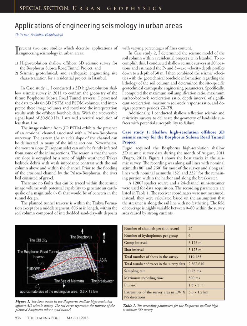
Case study 1: Shallow high-resolution offshore 3D seismic survey for the Bosphorus Subsea Road Tunnel ProjectFugro acquired the Bosphorus high-resolution shallow 3D seismic survey data during the month of August, 2011 (Fugro, 2011). Figure 1 shows the boat tracks in the seis-mic survey. The recording was along sail lines with nominal azimuths 80˚ and 260˚ for most of the survey and along sail lines with nominal azimuths 152˚ and 332˚ for the remain-ing portion within the harbor and along the breakwater.

A 1200J sparker source and a 24-channel mini-streamer were used for data acquisition. The recording parameters are listed in Table 1. The receiver coordinates were not measured; instead, they were calculated based on the assumption that the streamer is along the sail line with no feathering. The fold of coverage is highly variable between 0–80 within the survey area caused by strong currents.

Figure 1. The boat tracks in the Bosphorus shallow high-resolution offshore 3D seismic survey. The red curve represents the traverse of the planned Bosphorus subsea road tunnel.

Table 1. The recording parameters for the Bosphorus shallow high-resolution 3D survey.

Number of channels per shot record 24

Number of hydrophones per group 6

Group interval 3.125 m

Shot interval 3.125 m

Total number of shots in the survey 119,485

Total number of traces in the survey data 2,867,640

Sampling rate 0.25 ms

Maximum recording time 500 ms

Bin size 1.5 × 5 m

Extremities of the survey area in EW X NS directions

3.6 × 1.2 km

March 2013 The Leading Edge 937

U r b a n g e o p h y s i c s U r b a n g e o p h y s i c s

and then created the stacking velocity field along the traverse of the inline under consideration. I used the inline velocity fields to create the 3-D velocity field shown in Figure 3. I then performed Dix conversion of the 3-D stacking velocity field to create the 3-D interval field for 3-D PSDM as shown in Figure 4.

Next, I stacked the data using the 3-D stacking velocity field shown in Figure 3. The strong water-bottom multiples could not have been attenuated by the velocity discrimina-tion between primaries and multiples since a short streamer was used in data acquisition. Instead, I used the periodicity of multiples and applied poststack spiking deconvolution with a long operator length to attenuate strong water-bottom and peg-leg multiples. Spiking deconvolution (160-ms operator length and 0.25 ms prediction lag) followed by bandpass fil-tering (30,60–800,960 Hz) also was aimed at restoring the flat spectrum within the recoverable signal band.

I performed 3-D prestack Kirchhoff time migration of the signal-processed shot gathers using the 3-D stacking velocity field shown in Figure 3, and 3-D prestack Kirchhoff depth migration using the 3-D interval velocity field shown in Fig-ure 4. The highly variable fold of coverage, the uncertainties associated with the assumptions made regarding the receiver coordinates, and the failure of the Kirchhoff method to image ultra-shallow events had a detrimental effect on the quality of the image volumes obtained from both migrations.

Albeit I eventually did use the depth image volume in

Data analysisThe data were processed using the recording sampling rate of 0.25 ms. The signal processing sequence includes:

1) trace balancing of all the traces in the shot records to a common rms level,

2) wide bandpass filtering (30,60–800,960 Hz) to remove the low-frequency swell noise caused by strong currents, water waves and intensive maritime traffic, and high-fre-quency ambient noise,

3) geometric spreading correction by t-squared scaling, 4) bottom tapering of amplitudes to reduce the ambient

noise at late times, 5) spiking deconvolution (48-ms operator length and 0.25

ms prediction lag) to compress the source wavelet to a spike at zero lag and flatten the spectrum within the recov-erable signal band, and

6) wide bandpass filtering (30,60–800,960 Hz).

Figure 2 shows a field record before and after the applica-tion of the signal processing sequence. The central frequency of the recoverable signal band is about 400 Hz after signal processing; thus, I attained a vertical resolution of less than 1 m.

Following signal processing, I performed velocity analy-sis. I applied NMO correction to prestack data using a range of constant velocities and created stacking velocity cubes (Yilmaz, 2001) for selected inlines (in the E-W direction) at 100-m intervals in the crossline direction. Based on the highest-stack-amplitude criterion, I picked the stacking ve-locities from the three cross-sections of each velocity cube,

Figure 2. A 24-trace shot gather from the 3D survey before (a) and after (b) signal processing. The noise associated with point scatterers at the water bottom or marine vessels can have linear or curved moveout as indicated by the red arrows, depending on the location with respect to the streamer. Such noise is difficult to remove and can also manifest itself in the migrated data.

Figure 3. The 3D stacking velocity field viewed from south to north.

Figure 4. The 3D interval velocity field viewed from south to north derived from Dix conversion of the 3D velocity field in Figure 3.



visualizing the interpreted horizons, the actual interpretation was made using the image volume from 3-D poststack Stolt migration. I performed 3-D constant-velocity Stolt migration to ensure preserving the relative amplitudes and signal band, and collapse diffractions and image steeply dipping events at ultra-shallow depths.

InterpretationI began the interpretation session by reviewing the borehole data along the planned tunnel traverse. The simplified soil column description and well tops from one of the boreholes are listed in Table 2. The borehole information (Fugro, 2010) indicates a soil column of sand-clay-silt with varying percent-ages, both vertically and laterally. Most of the geotechnical borings have reached the soil-bedrock interface and entered the bedrock Trakya formation composed of primarily grey-wacke sandstone.

I correlated the well-tops with the major seismic events —Top-Trakya bedrock, Top-gravel, and Top-slope-gravel. (Figure 5). The erosional channels for the present-day Bos-phorus waterway and the Palaeo-Bosphorus waterway are clearly observed in most inline sections. Maximum depth of the channel at the trough is about 150 m from the sea level. Maximum water depth of the present-day Bosphorus water-way within the survey area is 60 m.

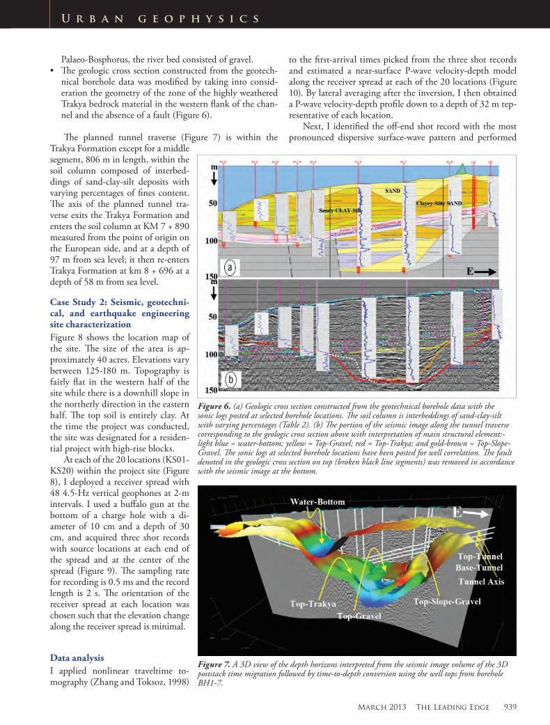
The main structural elements were also interpreted from the image section along the tunnel traverse extracted from the image volume. Figure 6 shows the portion of the seismic image along the tunnel traverse corresponding to the geo-

logic cross section constructed from the borehole data with the sonic logs posted at selected borehole locations and with interpretation of main structural elements—water-bottom, Top-Trakya, Top-Gravel, and Top-Slope-Gravel. The soil column is composed of interbeddings of sand-clay-silt with varying percentages (Table 2). The top of the zone associated with the highly weathered sandstone Trakya bedrock mate-rial has also been marked. The sonic logs at selected borehole locations indicate a seismically monotonous soil column with insignificant vertical velocity variations, but exhibit a strong contrast at Top-Gravel and Top-Trakya levels.

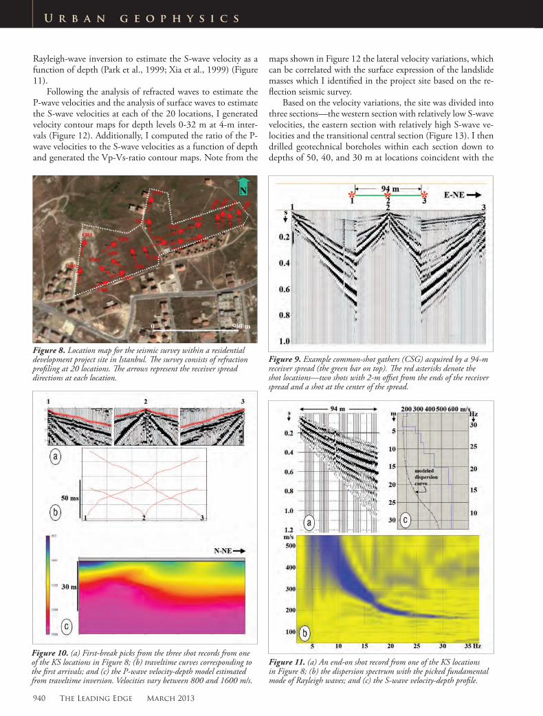
Time horizons were interpreted for the water-bottom, top-Trakya, Top-Gravel, and Top-Slope-Gravel from the seis-mic image volume of 3D poststack time migration. The well-tops from Borehole BH1-7 were then used to convert these time horizons to depth horizons. Figure 7 show a 3D view of the depth horizons.

Conclusions• The image volume exhibits the presence of an erosional

channel associated with a Palaeo-Bosphorus waterway. Maximum depth of the channel is about 150 m from sea level. Prior to the flooding of the erosional channel by the

Table 2. Simplified BH1-6 borehole data. The left column represents the layer thickness (m). The center column represent the top of the layer (m) measured from sea level.

Layer thick-ness (m)

Top Layer (m)

0.0-5.1 23.5 calcareous silica fine-to-medium SAND

5.1-12.4 28.6 firm sandy calcareous lean SILT12.4-30.2 35.9 silty calcareous silica fine SAND30.2-38.5 53.7 sandy calcareous lean SILT38.5-46.2 62.0 dense silicious carbonate fine

SAND46.2-51.6 69.7 calcareous lean CLAY with sand51.6-75.3 75.1 dense calcareous fine SAND75.3-77.5 98.8 GRAVEL77.5-85.0 101.0 stiff calcareous lean CLAY with

sand85.0-92.7 108.5 dense SAND92.7-112.1 116.2 calcareous fat CLAY with coarse

gravel112.1-117.7 135.6 dense calcareous silica medium

SAND117.7-120.0 140.5 SANDSTONE

143.5 End of boreholeFigure 5. (a) An inline section from the 3D Stolt migration volume that shows the present-day Bosphorus Channel and the Palaeo-Bosphorus Channel. The lateral extent of the section is about 2000 m and the time interval shown is 0-200 ms which corresponds to depth interval 0–150 m. (b) Zoomed-in portion of the inline section in (a), interpreted for the main structural elements—top-Trakya, top-gravel, and top-slope gravel. The dotted red horizon segment represents the top of the zone associated with the in-situ highly weathered Trakya bedrock material. The lateral extent of the section is more than 1000 m. The time interval shown is 0-200 ms which corresponds to depth interval 0-150 m.



Palaeo-Bosphorus, the river bed consisted of gravel.• The geologic cross section constructed from the geotech-

nical borehole data was modified by taking into consid-eration the geometry of the zone of the highly weathered Trakya bedrock material in the western flank of the chan-nel and the absence of a fault (Figure 6). The planned tunnel traverse (Figure 7) is within the

Trakya Formation except for a middle segment, 806 m in length, within the soil column composed of interbed-dings of sand-clay-silt deposits with varying percentages of fines content. The axis of the planned tunnel tra-verse exits the Trakya Formation and enters the soil column at KM 7 + 890 measured from the point of origin on the European side, and at a depth of 97 m from sea level; it then re-enters Trakya Formation at km 8 + 696 at a depth of 58 m from sea level.

Case Study 2: Seismic, geotechni-cal, and earthquake engineering site characterizationFigure 8 shows the location map of the site. The size of the area is ap-proximately 40 acres. Elevations vary between 125-180 m. Topography is fairly flat in the western half of the site while there is a downhill slope in the northerly direction in the eastern half. The top soil is entirely clay. At the time the project was conducted, the site was designated for a residen-tial project with high-rise blocks.

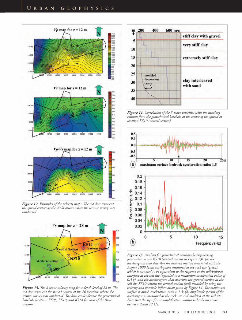
At each of the 20 locations (KS01-KS20) within the project site (Figure 8), I deployed a receiver spread with 48 4.5-Hz vertical geophones at 2-m intervals. I used a buffalo gun at the bottom of a charge hole with a di-ameter of 10 cm and a depth of 30 cm, and acquired three shot records with source locations at each end of the spread and at the center of the spread (Figure 9). The sampling rate for recording is 0.5 ms and the record length is 2 s. The orientation of the receiver spread at each location was chosen such that the elevation change along the receiver spread is minimal.

Data analysisI applied nonlinear traveltime to-mography (Zhang and Toksoz, 1998)

to the first-arrival times picked from the three shot records and estimated a near-surface P-wave velocity-depth model along the receiver spread at each of the 20 locations (Figure 10). By lateral averaging after the inversion, I then obtained a P-wave velocity-depth profile down to a depth of 32 m rep-resentative of each location.

Next, I identified the off-end shot record with the most pronounced dispersive surface-wave pattern and performed

Figure 6. (a) Geologic cross section constructed from the geotechnical borehole data with the sonic logs posted at selected borehole locations. The soil column is interbeddings of sand-clay-silt with varying percentages (Table 2). (b) The portion of the seismic image along the tunnel traverse corresponding to the geologic cross section above with interpretation of main structural element:- light blue = water-bottom; yellow = Top-Gravel; red = Top-Trakya; and gold-brown = Top-Slope-Gravel. The sonic logs at selected borehole locations have been posted for well correlation. The fault denoted in the geologic cross section on top (broken black line segments) was removed in accordance with the seismic image at the bottom.

Figure 7. A 3D view of the depth horizons interpreted from the seismic image volume of the 3D poststack time migration followed by time-to-depth conversion using the well tops from borehole BH1-7.



Figure 11. (a) An end-on shot record from one of the KS locations in Figure 8; (b) the dispersion spectrum with the picked fundamental mode of Rayleigh waves; and (c) the S-wave velocity-depth profile.

Figure 8. Location map for the seismic survey within a residential development project site in Istanbul. The survey consists of refraction profiling at 20 locations. The arrows represent the receiver spread directions at each location.

Figure 9. Example common-shot gathers (CSG) acquired by a 94-m receiver spread (the green bar on top). The red asterisks denote the shot locations—two shots with 2-m offset from the ends of the receiver spread and a shot at the center of the spread.

Figure 10. (a) First-break picks from the three shot records from one of the KS locations in Figure 8; (b) traveltime curves corresponding to the first arrivals; and (c) the P-wave velocity-depth model estimated from traveltime inversion. Velocities vary between 800 and 1600 m/s.

Rayleigh-wave inversion to estimate the S-wave velocity as a function of depth (Park et al., 1999; Xia et al., 1999) (Figure 11).

Following the analysis of refracted waves to estimate the P-wave velocities and the analysis of surface waves to estimate the S-wave velocities at each of the 20 locations, I generated velocity contour maps for depth levels 0-32 m at 4-m inter-vals (Figure 12). Additionally, I computed the ratio of the P-wave velocities to the S-wave velocities as a function of depth and generated the Vp-Vs-ratio contour maps. Note from the

maps shown in Figure 12 the lateral velocity variations, which can be correlated with the surface expression of the landslide masses which I identified in the project site based on the re-flection seismic survey.

Based on the velocity variations, the site was divided into three sections—the western section with relatively low S-wave velocities, the eastern section with relatively high S-wave ve-locities and the transitional central section (Figure 13). I then drilled geotechnical boreholes within each section down to depths of 50, 40, and 30 m at locations coincident with the



Figure 12. Examples of the velocity maps. The red dots represent the spread centers at the 20 locations where the seismic survey was conducted.

Figure 13. The S-wave velocity map for a depth level of 28 m. The red dots represent the spread centers at the 20 locations where the seismic survey was conducted. The blue circles denote the geotechnical borehole locations KS05, KS10, and KS14 for each of the three sections.

Figure 14. Correlation of the S-wave velocities with the lithology column from the geotechnical borehole at the center of the spread at location KS10 (central section).

Figure 15. Analysis for geotechnical earthquake engineering parameters at site KS10 (central section in Figure 13): (a) the accelerogram that describes the bedrock motion associated with the August 1999 Izmit earthquake measured at the rock site (green), which is assumed to be equivalent to the response at the soil-bedrock interface at the soil site (upscaled to a maximum acceleration value of 0.3 g), and the accelerogram that describes the ground motion at the soil site KS10 within the central section (red) modeled by using the velocity and borehole information given by Figure 14. The maximum surface-bedrock acceleration ratio is 1.5; (b) amplitude spectra of the accelerograms measured at the rock site and modeled at the soil site. Note that the significant amplification within soil column occurs between 0 and 12 Hz.



Table 3. Geotechnical earthquake engineering parameters.

Section Maximum soil amplification ratio

Nautral period of the soil col-umn (s)

Maximum surface-bedrock accelera-tion ratio

Depth interval with significant acceleration (m)

Maximumsoil-rock re-sponse

Design spectrum periods TA–TB (s)

Western 2.2 0.4 1.3 0–10 1.3 0.05–0.60Central 2.4 0.3 1.5 0–15 2.4 0.05–0.55Eastern 2.8 0.15 1.7 0–10 2.1 0.05–0.65

center of the spreads KS05, KS10, and KS14, respectively.

Estimation of geotechnical earthquake engineering pa-rametersFor each section within the project site (western, central, and eastern as shown in Figure 13), the S-wave velocities within the soil column combined with the borehole lithology (Fig-ure 14) were used to determine the geotechnical earthquake engineering parameters.

I began with a rock-site SH accelerogram that describes the time history of the strong ground motion associated with the August 1999 Izmit earthquake (Yilmaz et al., 2006). Given the S-wave velocity-depth profile, the geotechnical borehole information, and the accelerogram that describes the ground motion at the rock site, I calculated the accelero-gram that simulates the ground motion at the soil site (Figure 15) for each of the three sections within the site. This one-dimensional site-response analysis was performed using a fre-quency-domain algorithm that models the nonlinear material behavior of the soil column as an equivalent linear system (Bardet et al., 2000).

In earthquake engineering, the soil response to an earthquake mo-tion is calculated based on the sce-nario that corresponds to a maximum possible peak ground acceleration that may occur at a location (Kram-er, 1996). Hence, the accelerogram at the rock site (equivalently, at the soil-bedrock interface), was actually upscaled to a maximum value of 0.3g before the modeling of the accelero-gram at the soil sites within each sec-tion (KS05, KS10, and KS14).

From Figure 15, I determined for each section (Figure 13) the ratio of the maximum ground acceleration at the soil site to the maximum ac-celeration at the soil-bedrock inter-face—often referred to as maximum surface-bedrock acceleration ratio. For each section, I also computed the maximum acceleration as a function of depth, and determined the depth range for which surface-bedrock ac-celeration ratio is significant (Figure 16). Specifically, as the bedrock mo-tion is upward propagated through

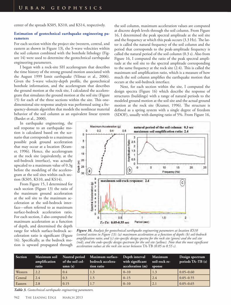
the soil column, maximum acceleration values are computed at discrete depth levels through the soil column. From Figure 16, I determined the peak spectral amplitude at the soil site and the frequency at which this peak occurs (3.3 Hz). The lat-ter is called the natural frequency of the soil column and the period that corresponds to the peak-amplitude frequency is called the natural period of the soil column (0.3 s). Also from Figure 16, I computed the ratio of the peak spectral ampli-tude at the soil site to the spectral amplitude corresponding to the same frequency at the rock site (2.4). This is called the maximum soil amplification ratio, which is a measure of how much the soil column amplifies the earthquake motion that occurs at the soil-bedrock interface.

Next, for each section within the site, I computed the design spectra (Figure 16) which describe the response of structures (buildings) with a range of natural periods to the modeled ground motion at the soil site and the actual ground motion at the rock site (Kramer, 1996). The structure is defined as a spring system with a single degree of freedom (SDOF), usually with damping ratio of 5%. From Figure 16,

Figure 16. Analysis for geotechnical earthquake engineering parameters at location KS10 (central section in Figure 13): (a) maximum acceleration as a function of depth; (b) soil-bedrock amplification ratio; and (c) site-specific design spectra for the rock site (green) and the soil site (red), and the code-specific design spectrum for the soil site (yellow). Note that the most significant acceleration values at the rock site occur between TA-TB (0.05 to 0.55 s).



Figure 17. Location map for the shallow reflection seismic and resistivity surveys conducted within a residential development project site in Istanbul. The survey consists of reflection profiling along the line traverses YS05-10. The RS locations represent the center of the resistivity spreads. The two yellow curves represent the boundaries of the landslide masses delineated from the survey.

Figure 18. Seismic image from prestack depth migration of shot gathers along line traverse YS09 (Figure 17). The broken events inside the ellipses represent sand lenses embedded in the predominantly clay soil column. The sand lenses sealed by the clay form excellent aquifers for groundwater. Note the migration smiles near the left and right edges of the section.

Figure 19. The velocity-depth models along the YS line traverses in Figure 17. The white line segments represent the landslide failure surfaces and the layers above represent the landslide masses with susceptibility to be triggered by an earthquake or heavy rainfall.

I determined the maximum of the response spectra at the ground level and soil-bedrock interface, and computed the maximum soil-rock response as the spectral acceleration ra-tio (2.4). I also determined the design spectrum periods TA-TB (0.05-0.55 sec). TA and TB correspond to the minimum and maximum periods for which the spectrum is nearly flat. Outside the TA-TB bandwidth, the spectrum ramps down rapidly.

Listed in Table 3 are the geotechnical earthquake engi-neering parameters for each of the three sections within the site. Combined with the parameters for the soil dynamics, such as the bearing capacity, these parameters were used by

the geotechnical engineer for soil classification and by the civil engineer for structural design of buildings.

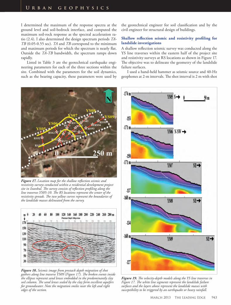
Shallow reflection seismic and resistivity profiling for landslide investigationsA shallow reflection seismic survey was conducted along the YS line traverses within the eastern half of the project site and resistivity surveys at RS locations as shown in Figure 17. The objective was to delineate the geometry of the landslide failure surfaces.

I used a hand-held hammer as seismic source and 40-Hz geophones at 2-m intervals. The shot interval is 2 m with shot



locations interleaved with the receiver locations. Example of a seismic image along a line traverse is shown in Figure 18. This image was generated by prestack depth migration of the shot gathers using the velocity-depth model estimated by trav-eltime tomography applied to the first-arrival times picked from the shot gathers (Figure 19). I delineated several land-slide failure surfaces from the velocity-depth models along the YS line traverses. Additionally, I observed low resistivity values at depths that correspond to the potential failure sur-faces. This suggests that the failure surfaces are saturated with water and therefore susceptible being trigerred by an earth-quake or a heavy rainfall.

ConclusionsSite investigations require multidisciplinary participation by the geologist, seismologist, geotechnical and earthquake en-gineers (Figure 20). The geotechnical earthquake engineer-ing parameters for each of the three sections within the site (Table 3) combined with the parameters for the soil dynam-ics, such as the bearing capacity, were used by the geotechni-cal engineer for soil classification and by the civil engineer for structural design of buildings. Based on the reflection

seismic survey at the residential project site, the geotechnical engineer was able to develop a geotechnical soil remediation program that involved building a drainage system to circum-vent potential landslide hazards.

The two case studies presented in this paper demonstrate successful applications of engineering seismology in urban ar-eas. Specifically, in major urban projects, geophysical methods help the geotechnical engineer design a geotechnical model of the soil column that can be used for soil remediation, and the civil engineer perform structural design of buildings by tak-ing into consideration the seismic properties and, if required, the earthquake engineering parameters of the soil column.

ReferencesBardet J., K. Ichii, and C. Lin, 2000, Manual of EERA: a computer

program for equivalent-linear earthquake site response analysis of layered soil deposits: University of Southern California.

Fugro, 2010, The Bosphorus geotechnical borings report: Avrasya Tüneli İşletme İnşaat ve Yatırım AŞ (ATAŞ), Istanbul.

Fugro, 2011, The Bosphorus 3-D seismic data acquisition report: Avrasya Tüneli İşletme İnşaat ve Yatırım AŞ (ATAŞ), Istanbul.

Kramer, S. L., 1996, Geotechnical earthquake engineering: Prentice-Hall.

Park, C. B., R. D. Miller, and J. Xia, 1999, Multichannel analysis of surface waves: Geophysics, 64, no. 3, 800–808, http://dx.doi.org/10.1190/1.1444590.

Xia, J., R. D. Miller, and C. B. Park, 1999, Estimation of near-surface shear-wave velocity by inversion of Rayleigh waves: Geophysics, 64, no. 3, 691–700, http://dx.doi.org/10.1190/1.1444578.

Yilmaz, O., 2001, Seismic data analysis: SEG, http://dx.doi.org/10.1190/1.9781560801702.

Yilmaz, O., M. Eser, and M. Berilgen, 2006, A case study for seis-mic zonation in municipal areas: The Leading Edge, 25, no. 3, 319–330, http://dx.doi.org/10.1190/1.2184100.

Zhang, J., and M. N. Toksoz, 1998, Nonlinear refraction traveltime tomography: Geophysics, 63, no. 5, 1726–1737, http://dx.doi.org/10.1190/1.1444468.

Acknowledgments: Thanks to Avrasya Tüneli İşletme İnşaat ve Yatırım AŞ (ATAŞ) for permission to publish this paper, to the Hanyapi Real Estate Development Corp., Istanbul and Professor Ahmet M. Işıkara for the opportunity to conduct the integrated site investigation project and for permission to publish the results.

Corresponding author: [email protected]

Figure 20. Site investigations require multidisciplinary participation by the geologist, seismologist, geotechnical and earthquake engineers. The seismologist defines the geometry and the seismic velocities of the soil column, the geomorphologist determines the soil pedology, and the geotechnical engineer determines the dynamic properties of the soil column. The soil geometry, the soil pedology, and the soil dynamics constitute the geotechnical model of the soil column, which is then used by the geotechnical engineer for geotechnical design for soil remediation.

applications of engineering seismology in urban areas of engineering...then performed dix conversion...

Documents