pdf, 407kb - crawford school of public policy - australian national
TRANSCRIPT

Working Papers in Trade and Development
Gasoline prices, gasoline consumption, and
new-vehicle fuel economy: Evidence for a large
sample of countries
Paul J. Burke and
Shuhei Nishitateno
December 2011 Working Paper No. 2011/15
Arndt-Corden Department of Economics Crawford School of Economics and Government
ANU College of Asia and the Pacific


Gasoline prices, gasoline consumption, and new-vehicle fuel economy: Evidence for a large
sample of countries
Paul J Burke Arndt-Corden Department of Economics
Crawford School of Economics and Government The College of Asia and the Pacific
And
Shuhei Nishitateno
Arndt-Corden Department of Economics Crawford School of Economics and Government
The College of Asia and the Pacific
Corresponding Address : Paul J Burke
Arndt-Corden Department of Economics Crawford School of Economics and Government
The College of Asia and the Pacific The Australian National University
Coombs Building 9 Canberra ACT 0200
Email: [email protected]
December 2011
Working Paper No. 2011/15

This Working Paper series provides a vehicle for preliminary circulation of research results in the fields of economic development and international trade. The series is intended to stimulate discussion and critical comment. Staff and visitors in any part of the Australian National University are encouraged to contribute. To facilitate prompt distribution, papers are screened, but not formally refereed.
Copies may be obtained at WWW Site http://www.crawford.anu.edu.au/acde/publications/

1
Gasoline prices, gasoline consumption, and new-vehicle fuel economy: Evidence for a large sample of countries
Paul J. Burke* and Shuhei Nishitateno
Crawford School of Economics & Government, Australian National University, Canberra,
ACT 0200, Australia
* Corresponding author. E-mail: [email protected]. Telephone: +61 2 6125 6566
December 2011
Abstract
Countries differ considerably in terms of the price drivers pay for gasoline. This paper uses data for a large sample of countries to provide new evidence on the implications of these differences for the consumption of gasoline for road transport and the fuel economy of new vehicles. To address the potential for simultaneity bias in ordinary least squares estimation, we use a country’s oil reserves as an instrument for its average gasoline pump price. We obtain estimates of the long-run price elasticity of gasoline demand of between –0.2 and –0.4, a smaller elasticity than most existing estimates. The results also indicate that higher gasoline prices induce consumers to substitute to vehicles that are more fuel-efficient, with an estimated elasticity of +0.2. While gasoline demand and fuel economy are both inelastic with respect to gasoline prices, there is considerable scope for low-price countries to achieve gasoline savings and vehicle fuel economy improvements via reducing gasoline subsidies and/or increasing gasoline taxes.
Keywords: vehicle, gasoline demand, fuel use, fuel economy, gasoline price
JEL classification: N70, L91, Q43, Q48
2
Gasoline prices, gasoline consumption, and new-vehicle fuel economy: Evidence for a large sample of countries
1. Introduction
By sales, the most popular new vehicles in Japan in 2008 were the Suzuki Wagon R and the
Daihatsu Move, which are both classed as mini cars. The most popular vehicles in the United
States (US) were the Ford F-Series and the Chevrolet Silverado, both classed as “pickup”
trucks (Marklines 2011). The Wagon R and Move have much higher fuel economy ratings
than the F-Series and the Silverado. Per capita consumption of gasoline for driving in Japan is
only 29% of that in the US (World Bank 2011a). This paper focuses on the importance of
differentials in gasoline pump prices in explaining these large differences in both gasoline use
and vehicle fuel economy between countries.
The large variation in gasoline pump prices between countries is shown in Figure 1, which
uses data from a survey of international gasoline prices carried out by GTZ (2009). Gasoline
tends to be cheapest in oil-rich countries, which are represented by the shaded dots in the
Figure. The average gasoline pump price was only 2 US cents per liter in Venezuela in 2008,
a small fraction of the price prevailing in the median country (111 US cents per liter) or the
country with the highest price (Eritrea, 253 US cents per liter). The gasoline price in Japan
(142 US cents per liter in 2008) is more than double the average price in the US (56 cents).
-Fig. 1 here-
This paper presents estimates of the price elasticity of demand for both gasoline use and new-
vehicle fuel economy for a large sample of countries. Both cross-sectional and pooled cross-

3
section time-series models are estimated using data covering the period 1995-2008. To
address the potential simultaneity bias present in ordinary least squares (OLS) estimation, we
present specifications that use a country’s in-ground proved oil reserves as an instrument for
the local gasoline price. Oil reserves are negatively correlated with the gasoline pump price
across countries, and serve as a “supply-curve shifter” capable of allowing the identification
of the parameters of the demand equations.1
In line with expectations, the results suggest that
higher gasoline prices both reduce per capita road-sector gasoline consumption and see
consumers substitute toward more fuel-efficient automobiles. The estimated price elasticities
are relatively small, but indicate that countries with very low gasoline prices could see
substantial gasoline savings and vehicle fuel efficiency gains by moving toward
internationally-normal gasoline price levels.
This paper adds to a large literature on measuring the price elasticity of demand for gasoline
and also the gasoline-price elasticity of vehicle fuel economy. The primary contributions are
the employment of a new instrumental variable (IV) approach and the use of newly-compiled
data on the fuel economy of new passenger vehicles. The use of an IV approach means that
this paper has a greater focus on obtaining an internally-valid causal estimate of price impacts
than most papers in the literature (which typically use single-equation estimation techniques
such as OLS which ignore the potential endogeneity of gasoline prices). The fuel economy
data are country averages for large samples of new vehicles at the make-model-configuration
level of detail, as calculated by the IEA (2011). Estimations in this paper are also for a larger
sample of countries than used in prior contributions (132 in total for the gasoline consumption
1 The approach is similar to estimates of the elasticity of demand for agricultural products which use weather
conditions as an instrument for the price (see Angrist and Krueger 2001). Our strategy relies on exploiting cross-
country supply curve differences to identify the demand curve rather than intertemporal supply shocks.
4
specifications, including countries rarely included in gasoline demand studies, such as
Venezuela and Iran). The estimations cover recent years (to 2008) and control for additional
potential determinants of gasoline demand, such as vehicle fuel economy standards, vehicle
import tariff rates, and a measure of the importance of other forms of transport.
Road transport is an increasingly important sector, accounting for 14% of global energy use,
40% of global oil use, and 17% of global carbon dioxide (CO2) emissions from energy in
2008 (International Energy Agency [IEA] 2010a, 2010b). Evidence on the responsiveness of
consumers to gasoline price levels is of relevance to policymakers in light of heightening
concerns about oil scarcity and the environmental impacts of oil use, including global climate
change. Evidence on the importance of gasoline prices for gasoline use is of particular policy
relevance because gasoline prices have traditionally been subject to substantial government
influence. Indeed, taxes contribute a large share of the gasoline pump price in many countries,
and differences in tax rates make up a sizeable share of cross-country differences in gasoline
pump prices (Rietveld and van Woudenberg 2005).2 In other countries, such as Venezuela,
Saudi Arabia, Iran, and Indonesia, gasoline price subsidies represent a large drain on the
government budget.3
The results in this paper have implications for the potential efficacy of
price-based approaches for managing energy use in the transport sector, and more broadly.
The remainder of this paper is organized as follows. Section 2 presents an initial look at the
data on gasoline pump prices, gasoline consumption, and new-vehicle fuel economy. The
empirical approach is presented and the data are introduced in section 3. Section 4 presents 2 For instance, in 2008, taxes made up 63% of the final gasoline pump price in Germany, 56% in Portugal, 49%
in Korea, 39% in Japan, and 16% in the United States (IEA 2010c).
3 The international price for crude oil was 30 US cents per liter in November 2008. Countries with gasoline
prices below this level are applying very large subsidies to the use of gasoline for driving.

5
the results and discusses robustness issues. Section 5 relates our results to prior estimates. The
final section concludes.
2. Gasoline prices and consumption: Initial evidence
Figure 2 plots per capita road-sector gasoline consumption against the gasoline pump price
for 131 countries for the year 2008 (with both variables measured in natural logarithms). An
inverse association between the two variables is apparent: countries with higher gasoline
prices tend to consume less gasoline within their road sectors. Nevertheless, the Figure also
reveals that per capita gasoline consumption varies notably even among countries with similar
gasoline pump prices. Additional variables, such as per capita income and a country’s
population density, need to be considered in explaining this variation.
-Fig. 2 here-
It should be expected that consumers react to high fuel prices by purchasing vehicles that are
more economical in their use of fuel. Yet there is much less information on average new-
vehicle fuel economy at the country level than there is on gasoline consumption. This paper
uses recently-released data on the fuel economy of newly-purchased vehicles, which are
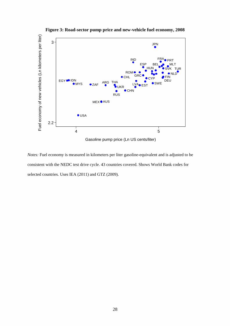
available for 43 countries (see section 3). The cross-country relationship between fuel
economy (measured by kilometers per liter gasoline-equivalent) and the gasoline pump price
for these countries in 2008 is presented in Figure 3. A positive association between the
variables is apparent: consumers in countries with higher gasoline prices appear to purchase
vehicles that have relatively higher fuel economy ratings. The US has the lowest average fuel
economy rating in the sample, consistent with our observation that some of the most popular

6
vehicles in the US are large vehicles. Japan has the highest fuel economy rating. Appendix A
presents lists of the ten most popular new vehicles by sales for both Japan and the US.
- Fig. 3 here-
This initial evidence is suggestive of an important effect of gasoline prices on both gasoline
consumption and new-vehicle fuel economy. Yet the scatterplots in Figures 2 and 3 do not
establish directional causality from gasoline prices to the y-axis variables and do not control
for other determinants of fuel use and passenger car fuel economy. The estimation framework
employed in this paper focuses on identifying the causal impact of gasoline prices on both
gasoline use and vehicle fuel economy.
3. Empirical approach and data
We model gasoline demand in the road sector (G) as follows:
, , , , ,( , , , )c t c t c t c t c tG f P Y D= X (1)
where P is the pump price for gasoline in country c in year t, Y is income per capita, D is
population density, and X is a vector of additional determinants. We adopt a log-log approach
so as to be able to estimate elasticities. The estimation equation is:
, , , , , ,ln ln ln lnc t c t c t c t c t c tG P Y Dα β γ δ φ ε= + + + + +X (2)
Our focus is on the price elasticity of demand for gasoline, β. Most prior studies on this price
elasticity have employed OLS estimation or other single-equation estimation approaches such
as generalized least squares. A potential problem with such approaches is that gasoline prices
are not exogenous: it is well known that OLS regression of quantities on prices fails to

7
identify either the demand curve or the supply curve (Angrist and Krueger 2001). While
gasoline is an internationally tradable commodity, within individual countries gasoline
markets are typically oligopolistic in nature. In such imperfectly competitive markets, the
supply curve is unlikely to be perfectly elastic, and so price levels may be affected by the
level of demand. The degree of competition in a country’s fuel distribution sector is difficult
to control for. Government gasoline tax/subsidy policies, which account for a large share of
cross-country differences in gasoline prices, may also be affected by the quantity of gasoline
being consumed. For example, a government may levy a higher gasoline tax if car
dependence is not particularly high (Hammar et al. 2004). Reverse causality from gasoline
consumption to the gasoline price would mean that OLS estimation of equation (2) will not
provide a consistent estimate of the price elasticity of demand for gasoline.
Econometric estimation is further complicated by the fact that the error term in equation (2)
may include other difficult-to-control-for variables which are correlated with the gasoline
price. One such variable may be the occurrence of political disturbances or civil conflicts,
which may disrupt oil supply chains and affect both the gasoline price and overall
consumption of gasoline. Other variables, such as the ruggedness of the terrain, are also hard
to adequately control for, but may influence both gasoline consumption (by affecting driving
requirements) and pump prices (by affecting gasoline distribution costs). In any of these
cases, OLS estimation of equation (2) would not be expected to provide a consistent estimate
of the causal impact of gasoline prices on gasoline consumption.
This paper employs IV estimation to address the potential endogeneity of gasoline pump
prices in equation (2) and obtain consistent coefficient estimates. We use a country’s in-
ground proved reserves of oil as an instrument for the gasoline price. As far as we are aware,

8
this is the first time oil reserves have been used as an instrument for gasoline pump prices.
Prior gasoline demand studies using IV approaches include Hughes et al. (2008), who use
supply-side production disruptions as sources of temporal variation in gasoline prices, and
Davis and Kilian (2010), who instrument for the gasoline price in the US using monthly
changes in gasoline tax rates at the state level. Our IV approach is better suited to obtaining
estimates of the long-run price elasticity of gasoline demand.
To serve as a good instrument, oil reserves must meet several conditions. First, they must be
strongly correlated with the gasoline price. As observed in Figure 1, oil-rich countries tend to
underprice gasoline on the domestic market, often as a means of sharing the rents from oil
extraction (Rietveld and van Woudenberg 2005). Oil-poor countries are more likely to impose
higher taxes on petrol because oil taxes provide a reliable revenue source, and to discourage
overconsumption of imported oil. We hypothesize that oil reserves are negatively correlated
with the gasoline pump price across countries.
The second requirement for oil reserves to act as a suitable instrument is that the proved
reserves of individual countries are not affected by annual road-sector gasoline consumption
in these countries. Proved oil reserves differ from actual oil endowments because oil
discovery requires exploration investment. It is unlikely that the level of gasoline
consumption in a country’s road sector has a strong impact on exploration activity in that
country, however, because countries’ marginal returns to oil discovery are similar given that
oil is an internationally traded commodity. Supply-side factors such as development level and
the security of property rights are likely to be much more important than transport-sector
demand conditions in explaining differences in exploration across countries. Current oil

9
reserves are affected by historical extraction in a country, but we obtain similar estimates
instrumenting with historical reserves estimates.
The final requirement for oil reserves to be a suitable instrument for pump prices is that they
are only correlated with gasoline consumption via the pump price (i.e. they are a supply-curve
shifter, but do not directly affect the demand curve; Angrist and Krueger 2001). We
acknowledge that oil reserves might affect gasoline consumption via other channels, and
control for measures of these channels where possible (see section 4.3). It is also possible that
citizens of oil-rich countries feel an additional entitlement to gasoline consumption which
influences their consumption decisions over and above the price they face. Despite the
difficulty of fully meeting the IV exclusion restriction, we believe that our IV estimates are a
worthwhile addition to the literature on modelling gasoline consumption.
We estimate equation (2) for a sample of 132 countries for each of the years 1995, 1998,
2000, 2002, 2004, 2006, and 2008, and for a pooled cross-section time-series dataset. (These
are the years for which gasoline price data are available for a reasonable number of countries
from GTZ (2009); data for some countries are missing for individual years.) The countries in
the sample represent 95% of the global population and 99% of global road-sector energy use
in 2008 (World Bank 2011a). To our knowledge, this is the largest sample of countries to be
included in a study on the determinants of vehicle gasoline demand. Many studies utilize
single-country time-series data (e.g. Akinboade et al. 2008 for South Africa). Some prior
studies also utilize data for samples of countries, with the largest sample we are aware of
consisting of 90 countries (Storchmann 2005).

10
Because our instrument does not display strong temporal variation, we focus primarily on the
cross-sectional estimations. We assume that countries are in long-run equilibrium and
interpret coefficient estimates from the cross-country specifications as long-run elasticities
(Baltagi and Griffin 1983). Because we have a relatively small-T panel and our instrument
does not vary much over time, we do not present estimates using country fixed effects. We
supplement our OLS and IV estimates with estimates using the between estimator, which can
provide consistent estimates of long-run relationships given standard assumptions about the
error term and its relationship with the explanatory variables (Stern 2010). We also present
estimates using historical gasoline price averages in recognition of the possibility that
gasoline demand and fuel economy adjust over time to price changes in a way that is not fully
picked up by a static specification.
Our estimation of the determinants of new-vehicle fuel economy (F) employs a similar
functional specification:
, , , , , ,ln ln ln ln Fc t c t c t c t c t c tF P Y Dϕ η κ λ τ ε= + + + + +X (3)
A strength of our analysis is that we use new data on new-vehicle fuel economy collated by
the IEA (2011) to measure F. The data are indicative country-level fuel economy averages
based on test drive results for samples of new vehicles at the make-model-configuration level.
The samples cover around three-quarters of new vehicle registrations in each country.
Because the fuel economy averages use ratings by vehicle configuration (i.e. sub-model), the
data provide a more accurate measure of average new-vehicle fuel economy than those used
in some prior studies (e.g. Wheaton 1982). (Fuel economy ratings of automobiles can vary
widely among vehicle models with different configurations e.g. engine and transmission
types.) The fuel economy data allow estimation for cross-sections of 42 countries in 2005 and

11
43 countries in 2008, and also a pooled sample using data for both years. The sample
represents around 90% of global vehicle sales, and includes more countries than prior studies
on the determinants of fuel economy (e.g. Clerides and Zachariadis 2008 used a sample of 18
countries). The IEA (2011) fuel economy data have not been used in prior regression
analyses.
There are several different test drive cycles in use internationally, and fuel economy readings
differ depending on the testing procedure used. To account for this, we adjust the IEA data for
differences in vehicle testing procedures using conversion factors provided by An and Sauer
(2004). The fuel economy data employed in this study are consistent with the New European
Drive Cycle (NEDC). We also convert the fuel economy ratings from liters per 100
kilometers to kilometers per liter to be consistent with the dominant approach to measuring
fuel economy in the literature (output/input).
Other data sources include the U.S. Energy Information Agency [EIA] (2011) and the World
Bank (2011a). Average income is measured using gross domestic product (GDP) per capita in
purchasing power parity (PPP) terms. The gasoline price data are in 2008 US dollars per liter,
and are not converted to PPP terms in keeping to the standard practice (and because PPP
differences between countries are taken into account by the GDP control). Summary statistics
for the year-2008 estimation dataset are presented in Table 1. A full list of data sources and
definitions for all variables is provided in Appendix B.
-Table 1 here-

12
Existing evidence indicates that gasoline prices affect gasoline consumption via influencing
vehicle ownership rates and driving distance, in addition to vehicle fuel economy choices
(Brons et al. 2008). Unfortunately, data availability currently precludes a full decomposition
of the channels via which gasoline prices affect gasoline consumption for a many-country
sample of the size used in this paper (see Small and van Dender 2007 for the case of the US).
(As for fuel economy, data on average driving distance at the country level are available for
less than one-third of countries in our sample, for example.)
Gasoline consumption and vehicle choice are part of a joint decision from among various
(transport and non-transport) consumption alternatives. Yet because the same explanatory
variables are included in equations (2) and (3), the efficient estimator is single-equation OLS
rather than system estimation (Greene 2000). Robust standard errors are presented. Standard
errors for the pooled cross-section time-series estimates are clustered at the country level to
account for within-country serial correlation.
4. Results
4.1. Results: Gasoline consumption
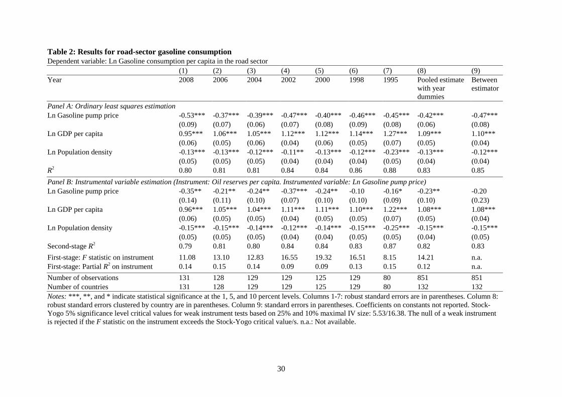
Results for estimations of equation (2) are presented in Table 2. Gasoline prices, GDP per
capita, and population density explain around 80% of the cross-country variation in gasoline
consumption. The OLS estimates (Panel A) suggest that the price elasticity of gasoline
demand is –0.4 to –0.5. Generally similar estimates are obtained for each of the seven years
and for the pooled OLS estimation and the between estimation for the period 1995-2008.
-Table 2 here-

13
The IV specifications (Panel B) provide slightly smaller price elasticity estimates, with a
range of –0.2 to –0.4 (for all years apart from 1995 and 1998). The IV estimations are also
less precise (i.e. have higher standard errors), although most are statistically different from
zero at the 5% significance level. The first stage of the IV regressions is satisfactory: the
coefficient on oil reserves per capita is negative (as expected), and oil reserves provide
sufficiently strong first-stage identification to allow confidence in the results. Specifically, the
null hypothesis of the Stock-Yogo weak instrument test of 25% maximal IV size is rejected
for each specification, and the stronger null of 10% maximal IV size is rejected for some
specifications. Similar estimates of the elasticities are obtained using IV estimators that are
robust to weak instruments, such as the Fuller (1977) estimator.
The results suggest an income elasticity of gasoline demand of +1.0 to +1.3. As found
elsewhere in the literature, the cross-country variation in per capita gasoline consumption is
thus much more sensitive to income differences than differences in gasoline pump prices. The
estimates also provide evidence that higher population density is associated with lower per
capita gasoline consumption, holding the gasoline price and per capita GDP constant.
4.2. Results: New-vehicle fuel economy
Results on the fuel economy of new vehicles are presented in Table 3. The OLS estimates
(Panel A) indicate that higher gasoline prices are associated with better fuel economy of new
vehicles, with an elasticity of +0.2. This confirms the positive association observed in Figure
3. The results also indicate that more densely-populated countries tend to use more fuel-
efficient vehicles. This accords with the intuition that drivers in countries with high
population density are likely to have to deal with narrower and more congested streets and

14
scarcer opportunities for vehicle parking than otherwise comparable countries, and so are
more likely to opt for smaller cars.
-Table 3 here-
Simultaneity bias is likely to be a smaller issue for the fuel economy regressions than for the
gasoline consumption regressions because fuel-economy choices are one step removed from
the gasoline price (whereas gasoline price and quantity are determined in the same market).
Nevertheless, results for fuel economy with the log gasoline price instrumented by oil
reserves per capita are presented in Panel B of Table 3. Unfortunately, per capita oil reserves
are a weak instrument for the log gasoline pump price for the smaller sample for which the
fuel economy data are available, as this sample excludes many oil-endowed countries. The
instrument fails to pass the Stock-Yogo weak instrument test in both the cross-sectional and
pooled samples. The second-stage estimates continue to indicate that higher gasoline prices
result in the purchase of vehicles with higher fuel economy ratings, yet these estimates are
associated with a high level of imprecision. Accordingly, our discussion of the results on fuel
economy will focus on the OLS estimations.
4.3. Robustness
It is important to consider robustness issues. The first is that the process of adjustment to price
changes requires time, and so a static representation might underestimate long-run price
elasticities. To consider this issue, we estimate the specifications for the cross-sectional
sample using the 1998-2008 average price instead of the 2008 price.4
4 Additional lags of the log gasoline price are statistically insignificant if included in the year-2008 regression.
The results for gasoline
consumption are reported in columns 1-2 of Table 4. The estimated elasticities are slightly

15
larger in this estimation, with the IV estimate of the long-run price elasticity of gasoline
consumption being –0.4. The second issue to consider is that in many countries drivers are
increasingly using diesel to fuel their vehicles. Columns 3-4 of Table 4 present estimates of
the combined demand for gasoline and diesel, using the average of the gasoline and diesel
pump prices as the primary explanatory variable. The estimated elasticities are somewhat
smaller than those presented in column 1 of Table 2, most likely because drivers are left with
fewer substitution possibilities once diesel is also included in the demand equation. Columns
5-6 of Table 4 include OLS results for new-vehicle fuel economy using the historical and
gasoline-diesel average price variables. These fuel economy results are similar to those
obtained in Table 3.
-Table 4 here-
An important issue with respect to the IV results in Table 2 is that oil reserves may affect
gasoline consumption through channels other than the gasoline price, and so violate the IV
exclusion restriction. Oil reserves may affect government policies related to the transport
sector, such as vehicle import tariffs or the use of alternative fuels, for instance. (Oil-poor
countries may seek to restrict car imports and/or support biofuels to reduce gasoline import
requirements.) To attempt to minimize this possibility, Table 5 presents estimates for the
year-2008 cross-section that control for additional variables that might be correlated with
gasoline consumption and also potentially correlated with oil reserves. Specifically, Table 5
controls for measures of national new-vehicle fuel economy standards (using data provided by
the International Council on Clean Transportation [ICCT] 2011), a measure of the availability
of alternative transport options (proxied by the non-road sector share of transport energy), a
measure of the availability of alternative sources of fuel for the road sector, the average tariff

16
level for new vehicle imports, and a dummy for whether the country was an early ratifier of
the Kyoto Protocol (a proxy of environmental policies). Table 5 also uses alternative
measures of income: gross national income (GNI) and gross domestic income, terms-of-trade
adjusted (GDI).
-Table 5 here-
The OLS and IV estimates of the price elasticity of gasoline demand and of new-vehicle fuel
economy remain generally similar across the specifications in Table 5, and remain
significantly different from zero in all but the IV estimate for gasoline consumption using
GDI per capita (column 6). Interestingly, we find no evidence that countries with higher fuel
economy standards are likely to have more fuel-efficient vehicles or use less gasoline in road
transport, although because fuel economy standards are not exogenous, the estimates on this
variable are unlikely to represent a causal effect. (The effect of standards is better identified in
time-series studies, which need to focus on smaller groups of countries due to limitations on
gasoline price data; see Clerides and Zachariadis 2008, for instance.) Countries in which
drivers have alternative fuel options (e.g. Brazil, which uses a large amount of bio energy as a
transport fuel) tend to have lower per capita demand for gasoline. The estimates also indicate
that higher border tariffs are associated with lower gasoline demand, most likely because
fewer people are able to afford their own vehicle. We find no evidence that early ratification
of the Kyoto Protocol affected year-2008 gasoline consumption or vehicle fuel economy
decisions.
A final issue to consider with respect to the IV estimates is that current oil reserves are
affected by historical extraction within a country, and extraction is likely to be higher in

17
countries with high gasoline demand. If this is the case, the exogeneity of the instrument
could be called into question. To address this, we ran additional specifications using historical
(1980) reserves as an instrument for the 2008 log gasoline pump price. We obtain very similar
estimates using this approach, with an estimated price elasticity of gasoline demand of –0.4.
(Results available on request.)
5. Relating the results to prior studies
There is a voluminous literature on the price responsiveness of gasoline consumption.
Reviews and meta-analyses of this literature include Espey (1998), Graham and Glaister
(2002), Goodwin et al. (2004), Basso and Oum (2007), Brons et al. (2008), Dahl (in press),
and Havranek et al. (in press). Existing evidence indicates that road-sector gasoline demand is
inelastic, reflecting the relative lack of alternatives to gasoline use. Our estimates are smaller
than the median long-run price elasticity of gasoline demand reported in most studies, with
most estimates being in the range –0.6 to –0.9 (Graham and Glaister 2002, Goodwin et al.
2004, Brons et al. 2008). Nevertheless, our estimates are not dissimilar to the long-run price
elasticity estimates obtained in some papers using cointegration techniques, such as Bentzen
(1994), Eltony and al-Mutairi (1995), Ramanathan (1999), and Akinboade et al. (2008).
Espey’s (1998) meta-analysis reports that the median estimate of the long-run price elasticity
of gasoline demand is –0.4, which is similar to our OLS estimates (but, in absolute value
terms, larger than most of our IV estimates). Dahl (in press) finds a median gasoline price
elasticity of –0.3 for models employing static estimation equations as we have here, which is
similar to our IV estimates. Our estimates are also consistent with recent meta-analysis
evidence from Havranek et al. (in press), who estimate an average long-run price elasticity of
gasoline demand of –0.3 after adjusting for publication bias. Our results thus serve to shore-

18
up Havranek et al.’s inference that gasoline consumption is more price inelastic than is
regularly believed.
Our estimate of the elasticity of new-vehicle fuel economy with respect to the gasoline pump
price is similar to that obtained in an eight-country study by Espey (1996), although Espey
uses fleet-wide fuel economy generated using top-down data based on kilometers travelled
and recorded fuel use. Our estimate is smaller than the gasoline price elasticities for fleet-wide
fuel economy of Wheaton (1982) and Johansson and Schipper (1997), and is also smaller than
some of the long-run gasoline price elasticities of vehicle fuel economy reported by Clerides
and Zachariadis (2008). The estimate here is consistent with the long-run gasoline price
elasticity of new-vehicle CO2 emissions intensity in European countries [+0.2] estimated by
Ryan et al. (2009), and exceeds Klier and Linn’s (2010) short-run estimate for new-vehicle
fuel economy of +0.1 using US data. The evidence that higher gasoline pump prices increase
the incentive to purchase vehicles that are more fuel-efficient is consistent with recent
evidence that higher fuel prices encourage the purchase of hybrid vehicles in the US
(Beresteanu and Li 2011, Gallagher and Muehlegger 2011).
6. Conclusion
This study has presented estimates of the impact of gasoline pump prices on road-sector
gasoline demand and the fuel economy of new passenger vehicles for a large sample of
countries. An IV estimation approach has been employed in order to identify a causal estimate
of the impact of gasoline prices on gasoline demand. The IV results suggest a long-run price
elasticity of gasoline demand of –0.2 to –0.4, which is smaller than many of the estimates in
the existing literature. The results suggest that gasoline pump prices affect vehicle choice
decisions also: a country with gasoline prices 10% higher than an otherwise similar country is

19
likely to have new vehicles of 2% higher fuel economy. Underlying country characteristics
such as population density and income level were also found to have important implications
for road-sector gasoline consumption and fuel economy.
While the estimated price elasticities of gasoline demand and fuel economy are relatively
small, the large differences in fuel prices between countries account for an important share of
the differences in gasoline consumption and fuel economy. A simple counterfactual is
informative: the estimation in column 1 of Table 3 indicates that a shift to Japan-level
gasoline prices in the US would result in an improvement in the fuel economy of new vehicles
in the US of around one-quarter, for instance (all else held constant). Because the US
accounts for 40% of global road-sector gasoline consumption (IEA 2010a), the estimates also
indicate that higher gasoline prices in the US would translate to a sizeable reduction in the
quantity of global oil demand.
There are a number of countries with gasoline prices much lower than those in the US, and on
a per capita basis these countries also tend to be relatively large consumers of gasoline.
Increasing gasoline prices is politically challenging, and would likely reduce the welfare of
some motorists. Nevertheless, the results in this study indicate that moves toward
internationally-normal gasoline prices in countries such as Venezuela and Iran would result in
substantial energy efficiency improvements in the transport sectors of these countries. Cutting
fossil fuel subsidies would also free up resources that could be used for other purposes.
Several international agencies have joined together in a Global Fuel Economy Initiative,
which has the aim of doubling new light-duty vehicle fuel economy (in terms of kilometers
per liter) globally by 2050 (see www.globalfueleconomy.org). The results in this paper

20
provide a timely reminder of the importance of price effects in stimulating the adoption of
energy-efficient technologies. Upward pressure on fuel prices over time would create an
impetus for vehicle fuel efficiency improvements and would complement other policy efforts
aimed at improving the energy efficiency of the transport fleet. Future research for large-N
country samples focusing on the effects of vehicle tax/subsidy policies on the adoption of
fuel-efficient cars would complement the focus on the importance of pump prices here.
Acknowledgements
We are grateful for comments from Prema-Chandra Athukorala, David Stern, and participants
at the 10th International Conference of the Japan Economic Policy Association. Funding was
received from the ANU Research School of Asia and the Pacific.

21
References
Akinboade, O., Emmanuel, Z., Kumo, W., 2008. The demand for gasoline in South Africa:
An empirical analysis using co-integration techniques. Energy Economics 30, 3222–3229.
An, F., Sauer, A., 2004. Comparison of Passenger Vehicle Fuel Economy and Greenhouse
Gas Emission Standards Around the World. Pew Center on Global Climate Change, Arlington
VA.
Angrist, J.D., Krueger, A.B., 2001. Instrumental variables and the search for identification:
From supply and demand to natural experiments. Journal of Economic Perspectives 15, 69–
85.
Baltagi, B.H., Griffin, J.M., 1983. Gasoline demand in the OECD: An application of pooling
and testing procedures. European Economic Review 22, 117–137.
Basso, L.J., Oum, T.H., 2007. Automobile fuel demand: A critical assessment of empirical
methodologies. Transport Reviews 27, 449–484.
Bentzen, J. 1994., An empirical analysis of gasoline demand in Denmark using cointegration
techniques. Energy Economics 16, 139–143.
Beresteanu, A., Li, S., 2011. Gasoline prices, government support, and the demand for hybrid
vehicles in the United States. International Economic Review 52, 161–182.
Brons, M., Nijkamp, P., Pels, E., Rietveld, P., 2008. A meta-analysis of the price elasticity of
gasoline demand. A SUR approach. Energy Economics 30, 2105–2122.
22
Clerides, S., Zachariadis, T., 2008. The effect of standards and fuel prices on automobile fuel
economy: An international analysis. Energy Economics 30, 2657–2672.
Dahl, C., In press. Measuring global gasoline and diesel price and income elasticities. Energy
Policy.
Davis, L.W., Kilian, L., 2011. Estimating the effect of a gasoline tax on carbon emissions.
Journal of Applied Econometrics 26, 1187–1214.
Eltony, M., al-Mutairi, N.H., 1995. Demand for gasoline in Kuwait: An empirical analysis
using cointegration techniques. Energy Economics 17, 249–253.
Espey, M., 1996. Watching the fuel gauge: An international model of fuel economy. Energy
Economics 18, 93–106.
Espey, M., 1998. Gasoline demand revisited: An international meta-analysis of elasticities.
Energy Economics 20, 273–295.
Fuller, W.A., 1977. Some properties of a modification of the limited information
estimator. Econometrica 45, 939–953.
Gallagher, K.S., Muehlegger, E., 2011. Giving green to get green? Incentives and consumer
adoption of hybrid vehicle technology. Journal of Environmental Economics and
Management 61, 1–15.

23
Goodwin, P., Dargay, J., Hanly, M., 2004. Elasticities of road traffic and fuel consumption
with respect to price and income: A review. Transport Reviews 34, 275–292.
Graham, D.J., Glaister, S., 2002. The demand for automobile fuel: A survey of elasticities.
Journal of Transport Economics and Policy 36, 1–25.
Greene, W.H., 2000. Econometric Analysis. 4th ed. Prentice Hall, New Jersey.
GTZ., 2009. International Fuel Prices 2009. 6th ed. Eschborn, Frankfurt.
Hammar, H., Lofgren, A., Sterner, T., 2004. Political economy obstacles to fuel taxation.
Energy Journal 25, 1–17.
Havranek, T., Irsova, Z., Janda, K., In press. Demand for gasoline is more price-inelastic than
commonly thought. Energy Economics.
Heston, A., Summers, R., Bettina, A., 2011. Penn World Table Version 7.0. Center for
International Comparisons of Production, Income and Prices, University of Pennsylvania.
Hughes, J.E., Knittel, C.R., Sperling, D., 2008. Evidence of a shift in the short-run price
elasticity of gasoline demand. Energy Journal 29, 113–134.
International Council on Clean Transportation., 2011. Global Comparison of Light-Duty
Vehicle Fuel Economy/GHG Emissions Standards. Washington DC.
International Energy Agency., 2010a. Energy Balances of Non-OECD Countries. Paris.

24
International Energy Agency., 2010b. CO2 Emissions from Fuel Combustion. Paris.
International Energy Agency., 2010c. Energy Prices and Taxes: Quarterly Statistics. Fourth
Quarter. Paris.
International Energy Agency., 2010d. Energy Balances of OECD Countries. Paris.
International Energy Agency., 2011. International comparison of light-duty vehicle fuel
economy and related characteristics. Working Paper 5/10. Paris.
Johansson, O., Schipper, L., 1997. Measuring the long-run fuel demand of cars: Separate
estimations of vehicle stock, mean fuel intensity, and mean annual driving distance. Journal of
Transport Economics and Policy 31, 277–292.
Klier, T., Linn, J., 2010. The price of gasoline and new vehicle fuel economy: Evidence from
monthly sales data. American Economic Journal: Economic Policy 2, 134–153.
Marklines., 2011. Automotive Information Platform. http://www.marklines.com.
Ramanathan, R., 1999. Short- and long-run elasticities of gasoline demand in India: An
empirical analysis using cointegration techniques. Energy Economics 21, 321–330.
Rietveld, P., van Woudenberg, S., 2005. Why fuel prices differ. Energy Economics 27, 79–
92.

25
Ryan, L., Ferreira, S., Convery, F., 2008. The impact of fiscal and other measures on new
passenger car sales and CO2 emissions intensity: Evidence from Europe. Energy Economics
31, 365–374.
Small, K.A., van Dender, K., 2007. Fuel efficiency and motor vehicle travel: The declining
rebound effect. Energy Journal 28, 25–51.
Stern, D.I., (2010). Between estimates of the emissions-income elasticity. Ecological
Economics 69, 2173–2182.
Storchmann, K., 2005. Long-run gasoline demand for passenger cars: The role of income
distribution. Energy Economics 27, 25–58.
U.S. Energy Information Administration., 2010. International Energy Statistics.
http://tonto.eia.doe.gov/cfapps/ipdbproject/IEDIndex3.cfm.
Wheaton, W.C., 1982. The long-run structure of transportation and gasoline demand. Bell
Journal of Economics 13, 439–454.
World Bank., 2011a. World Development Indicators. http://data.worldbank.org/data-
catalog/world-development-indicators.
World Bank., 2011b. World Integrated Trade Solution. http://wits.worldbank.org/wits/.

26
Figures
Figure 1: Gasoline pump price by country, 2008
Notes: 131 countries included, as per regression sample in Table 2. Uses GTZ (2009). Gasoline pump
prices are those collected in a mid-November survey. Shows World Bank codes for selected countries.

27
Figure 2: Road-sector pump price and gasoline consumption, 2008
Notes: Gasoline consumption is in the road sector. 131 countries covered. kgoe: kilogram of oil
equivalent. Shows World Bank codes for selected countries. Uses World Bank (2011a) and GTZ
(2009).
28
Figure 3: Road-sector pump price and new-vehicle fuel economy, 2008
EGY IDNMYS
USA
ZAF
AUSMEX
ARG THAUKR
RUS
CHL
CHN
IND
ROM
LVA EST
GRC
ESPHUN
CYPSWE
JPN
BEL
FRA
DEUFIN
SVK
PRTMLT
NLDTUR
2.2
3Fu
el e
cono
my
of n
ew v
ehic
les
(Ln
kilo
met
ers
per l
iter)
4 5
Gasoline pump price (Ln US cents/liter)
Notes: Fuel economy is measured in kilometers per liter gasoline-equivalent and is adjusted to be
consistent with the NEDC test drive cycle. 43 countries covered. Shows World Bank codes for
selected countries. Uses IEA (2011) and GTZ (2009).

29
Tables
Table 1: Summary statistics for 2008 dataset Variable Mean Standard
deviation Median Minimum Maximum Countries of
data availability
Ln Gasoline consumption per capita in the road sector (kilograms of oil equivalent)
4.42 1.47 4.65 0.01 7.05 131
Ln Gasoline pump price (current US cents per liter)
4.51 0.65 4.71 0.69 5.53 131
Ln GDP per capita (2005 international PPP dollars, chain series)
9.03 1.29 9.19 4.91 11.92 131
Ln Population density (per squared kilometer of land area)
4.20 1.42 4.36 0.53 8.84 131
Oil reserves per capita (tonnes oil equivalent)
119.40 560.11 0.45 0.00 5199.92 131
Ln Fuel economy of new vehicles (kilometers per liter)
2.65 0.12 2.67 2.27 2.95 43
Ln GNI per capita (international PPP dollars)
9.09 1.20 9.26 5.67 11.12 126
Ln GDI per capita (terms of trade adjusted, 2005 PPP dollars)
9.05 1.30 9.16 4.96 11.66 131
New-vehicle fuel economy standard (km per liter)
3.93 6.87 0.00 0.00 16.67 131
Non-road sector share of transport energy (%)
8.93 11.42 6.01 0.00 53.51 131
Other energy use in road transport (%) 7.45 5.60 5.43 2.09 35.50 131
Average tariff on vehicle imports (%) 16.83 17.16 10.00 0.00 100.00 127
Kyoto Protocol ratification prior to 2003 (dummy)
0.55 0.50 1.00 0.00 1.00 131
30
Table 2: Results for road-sector gasoline consumption Dependent variable: Ln Gasoline consumption per capita in the road sector (1) (2) (3) (4) (5) (6) (7) (8) (9) Year 2008 2006 2004 2002 2000 1998 1995 Pooled estimate
with year dummies
Between estimator
Panel A: Ordinary least squares estimation Ln Gasoline pump price -0.53*** -0.37*** -0.39*** -0.47*** -0.40*** -0.46*** -0.45*** -0.42*** -0.47***
(0.09) (0.07) (0.06) (0.07) (0.08) (0.09) (0.08) (0.06) (0.08) Ln GDP per capita 0.95*** 1.06*** 1.05*** 1.12*** 1.12*** 1.14*** 1.27*** 1.09*** 1.10***
(0.06) (0.05) (0.06) (0.04) (0.06) (0.05) (0.07) (0.05) (0.04) Ln Population density -0.13*** -0.13*** -0.12*** -0.11** -0.13*** -0.12*** -0.23*** -0.13*** -0.12*** (0.05) (0.05) (0.05) (0.04) (0.04) (0.04) (0.05) (0.04) (0.04) R2 0.80 0.81 0.81 0.84 0.84 0.86 0.88 0.83 0.85 Panel B: Instrumental variable estimation (Instrument: Oil reserves per capita. Instrumented variable: Ln Gasoline pump price) Ln Gasoline pump price -0.35** -0.21** -0.24** -0.37*** -0.24** -0.10 -0.16* -0.23** -0.20
(0.14) (0.11) (0.10) (0.07) (0.10) (0.10) (0.09) (0.10) (0.23) Ln GDP per capita 0.96*** 1.05*** 1.04*** 1.11*** 1.11*** 1.10*** 1.22*** 1.08*** 1.08***
(0.06) (0.05) (0.05) (0.04) (0.05) (0.05) (0.07) (0.05) (0.04) Ln Population density -0.15*** -0.15*** -0.14*** -0.12*** -0.14*** -0.15*** -0.25*** -0.15*** -0.15*** (0.05) (0.05) (0.05) (0.04) (0.04) (0.05) (0.05) (0.04) (0.05) Second-stage R2 0.79 0.81 0.80 0.84 0.84 0.83 0.87 0.82 0.83 First-stage: F statistic on instrument 11.08 13.10 12.83 16.55 19.32 16.51 8.15 14.21 n.a. First-stage: Partial R2 on instrument 0.14 0.15 0.14 0.09 0.09 0.13 0.15 0.12 n.a. Number of observations 131 128 129 129 125 129 80 851 851 Number of countries 131 128 129 129 125 129 80 132 132 Notes: ***, **, and * indicate statistical significance at the 1, 5, and 10 percent levels. Columns 1-7: robust standard errors are in parentheses. Column 8: robust standard errors clustered by country are in parentheses. Column 9: standard errors in parentheses. Coefficients on constants not reported. Stock-Yogo 5% significance level critical values for weak instrument tests based on 25% and 10% maximal IV size: 5.53/16.38. The null of a weak instrument is rejected if the F statistic on the instrument exceeds the Stock-Yogo critical value/s. n.a.: Not available.

31
Table 3: Results for the fuel economy of new vehicles Dependent variable: Ln Fuel economy of new vehicles (kilometers per liter) (1) (2) (3) (4) Year 2008 2005 Pooled
estimate with year dummy
Between estimator
Panel A: Ordinary least squares estimation Ln Gasoline pump price 0.20*** 0.15*** 0.16*** 0.19***
(0.06) (0.05) (0.05) (0.04) Ln GDP per capita -0.03 -0.08** -0.05* -0.06***
(0.03) (0.03) (0.03) (0.02) Ln Population density 0.04*** 0.06*** 0.05*** 0.05*** (0.01) (0.01) (0.01) (0.01) R2 0.61 0.60 0.57 0.62
Panel B: Instrumental variable estimation (Instrument: Oil reserves per capita. Instrumented variable: Ln Gasoline pump price) Ln Gasoline pump price 0.22 0.10 0.15 0.14
(0.14) (0.08) (0.09) (0.17) Ln GDP per capita -0.03 -0.06 -0.05 -0.05
(0.04) (0.04) (0.04) (0.06) Ln Population density 0.04* 0.06*** 0.05*** 0.05** (0.02) (0.01) (0.01) (0.02) Second-stage R2 0.61 0.58 0.57 0.61
First-stage: F statistic on instrument 0.96 3.76 2.33 n.a. First-stage: Partial R2 on instrument 0.03 0.08 0.05 n.a.
Number of observations 43 42 85 85 Number of countries 43 42 43 43 Notes: ***, **, and * indicate statistical significance at the 1, 5, and 10 percent levels. Estimates for year 2005 use the one-year lag of Ln Gasoline pump price due to the absence of data for 2005 for this variable. Columns 1, 2: robust standard errors are in parentheses. Column 3: robust standard errors clustered by country are in parentheses. Column 4: standard errors in parentheses. Coefficients on constants not reported. Stock-Yogo 5% significance level critical values for weak instrument tests based on 25% and 10% maximal IV size: 5.53/16.38. The null of a weak instrument is rejected if the F statistic on the instrument exceeds the Stock-Yogo critical value/s. n.a.: Not available.

32
Table 4: Results using alternative price measures, 2008 (1) (2) (3) (4) (5) (6) Dependent variable Ln Gasoline
consumption per capita in the road
sector
Ln (Gasoline + diesel) consumption per capita
in the road sector
Ln Fuel economy of new vehicles
OLS IV OLS IV OLS OLS Ln Gasoline pump price (historical real average)
-0.56*** -0.38*** 0.20** (0.10) (0.15) (0.06)
Ln Pump price (year-2008 gasoline and diesel average)
-0.24*** -0.22*** 0.17** (0.05) (0.08) (0.06)
Ln GDP per capita 1.00*** 0.99*** 0.96*** 0.96*** -0.05* -0.03 (0.06) (0.06) (0.05) (0.05) (0.03) (0.03)
Ln Population density -0.13*** -0.14*** -0.09*** -0.09*** 0.05*** 0.05*** (0.04) (0.05) (0.03) (0.03) (0.01) (0.01) R2 0.79 0.79 0.86 0.86 0.62 0.56 First-stage: F statistic on instrument - 13.21 - 12.06 - - First-stage: Partial R2 on instrument - 0.15 - 0.12 - - Number of countries 130 130 129 129 43 43 Notes: ***, **, and * indicate statistical significance at the 1, 5, and 10 percent levels. Robust standard errors are in parentheses. Coefficients on constants not reported. Stock-Yogo 5% significance level critical values for weak instrument tests based on 25% and 10% maximal IV size: 5.53/16.38. The null of a weak instrument is rejected if the F statistic on the instrument exceeds the Stock-Yogo critical value/s. IV estimations use oil reserves per capita as an instrument for the relevant price variable. The historical gasoline pump price averages the real pump price in the years 1998, 2000, 2002, 2004, 2006, and 2008, and uses linear interpolations of the log price in the case of missing price data. Early historical or diesel prices are not available for several countries in the sample.

33
Table 5: Results with additional controls and alternative income measures, 2008 (1) (2) (3) (4) (5) (6) (7) (8) (9) Dependent variable Ln Gasoline consumption per capita in the road sector Ln Fuel economy of new vehicles OLS IV OLS IV OLS IV OLS OLS OLS Ln Gasoline pump price -0.70*** -0.43** -0.71*** -0.43*** -0.68*** -0.26 0.21*** 0.22*** 0.21***
(0.14) (0.22) (0.15) (0.11) (0.14) (0.21) (0.08) (0.08) (0.08) Ln GDP per capita 0.83*** 0.88*** -0.05
(0.08) (0.09) (0.03) Ln GNI per capita 0.93*** 0.97*** -0.06
(0.07) (0.08) (0.04) Ln GDI per capita 0.82*** 0.90*** -0.05 (0.07) (0.10) (0.03) Ln Population density -0.13*** -0.15*** -0.11** -0.13** -0.11*** -0.14*** 0.04** 0.04* 0.04** (0.04) (0.04) (0.05) (0.05) (0.04) (0.04) (0.02) (0.02) (0.02) New-vehicle fuel economy standard (km per liter) 0.02* 0.01 0.00 -0.00 0.02* 0.01 -0.00 -0.00 -0.00 (0.01) (0.01) (0.01) (0.01) (0.01) (0.01) (0.00) (0.00) (0.00) Non-road sector share of transport energy (%) 0.00 -0.00 0.00 0.00 0.00 -0.00 -0.00 -0.00 -0.00 (0.01) (0.01) (0.01) (0.01) (0.01) (0.01) (0.00) (0.00) (0.00) Other energy use in road transport (%) -0.02** -0.02** -0.02* -0.02** -0.02* -0.02** -0.00 -0.00 -0.00 (0.01) (0.01) (0.01) (0.01) (0.01) (0.01) (0.00) (0.00) (0.00) Average tariff on vehicle imports (%) -0.01** -0.01 -0.01*** -0.01* -0.01** -0.00 -0.00 -0.00 -0.00 (0.00) (0.00) (0.00) (0.00) (0.00) (0.00) (0.00) (0.00) (0.00) Kyoto Protocol ratification prior to 2003 (dummy) 0.04 -0.04 0.15 0.08 0.07 -0.05 0.03 0.03 0.03 (0.14) (0.15) (0.13) (0.13) (0.14) (0.16) (0.04) (0.04) (0.04) R2 0.82 0.81 0.83 0.82 0.82 0.80 0.63 0.63 0.63 First-stage: F statistic on instrument - 9.49 - 9.55 - 8.67 - - - First-stage: Partial R2 on instrument - 0.08 - 0.20 - 0.07 - - - Number of countries 127 127 122 122 127 127 43 43 43 Notes: ***, **, and * indicate statistical significance at the 1, 5, and 10 percent levels. Robust standard errors are in parentheses. Coefficients on constants not reported. Stock-Yogo 5% significance level critical values for weak instrument tests based on 25% and 10% maximal IV size: 5.53/16.38. The null of a weak instrument is rejected if the F statistic on the instrument exceeds the Stock-Yogo critical value/s. IV estimations use oil reserves per capita as an instrument for the Ln Gasoline pump price.

34
Appendix A – Most popular passenger vehicles in Japan and the United States, 2008
Rank Make Model Vehicle type Sales (volume, '000) Japan 1 Suzuki Wagon R Mini car 205 2 Daihatsu Move Mini car 190 3 Honda Fit (Jazz) Car 175 4 Daihatsu Tanto Mini car 159 5 Toyota Vitz (Yaris) Car 123 6 Toyota Corolla Car 115 7 Honda Life Mini car 97 8 Daihatsu Mira (Cuore) Mini car 85 9 Toyota Prius Car 73 10 Toyota Passo Car 73 Share of all sales (%) 26 United States 1 Ford Ford F-Series Light truck 516 2 Chevrolet Silverado Light truck 465 3 Toyota Camry Car 437 4 Honda Accord Car 373 5 Toyota Corolla Car 351 6 Honda Civic Car 339 7 Nissan Altima Car 270 8 Chevrolet Impala Car 266 9 Dodge Ram Light truck 246 10 Honda CR-V Light truck 197 Share of all sales (%) 26 Notes: Uses Marklines (2011).

35
Appendix B – Variable descriptions
Ln Gasoline consumption per capita in the road sector: Natural logarithm of road-sector
gasoline consumption per capita (kilograms of oil equivalent). World Bank (2011a).
Ln Gasoline pump price: Natural logarithm of the average gasoline retail pump price in year-
2008 US cents per liter of gasoline. Prices were collected in a survey carried out in mid-
November. GTZ (2009). The US GDP deflator from the World Bank (2011a) is used to
deflate prices.
Ln GDP per capita: Natural logarithm of GDP per capita in 2005 international purchasing
power parity dollars (chain series). Heston et al. (2011).
Ln Population density: Natural logarithm of the population per squared kilometer of land area.
World Bank (2011a).
Oil reserves per capita: Proved reserves of crude oil, tonnes oil equivalent per capita. U.S.
EIA (2011).
Ln Fuel economy of new vehicles (kilometers per liter): Natural logarithm of the average fuel
economy of new passenger vehicles in kilometers per liter gasoline-equivalent based on data
from fuel economy tests. Averages were calculated for representative samples of new vehicle
registrations by the IEA (2011), using data at the make-model-configuration level. For
Australia and the US, the fuel economy average covers some light commercial vehicles that
are commonly used as passenger vehicles. We have made the data NEDC-consistent by

36
adjusting the fuel economy ratings of Japan, Mexico, and the US using conversion factors
from An and Sauer (2004).
Ln GNI per capita: Natural logarithm of GNI per capita in international purchasing power
parity dollars. World Bank (2011a).
Ln GDI per capita: Natural logarithm of GDI per capita (terms of trade adjusted, 2005
international purchasing power parity dollars). Heston et al. (2011).
New-vehicle fuel economy standard (km per liter): Fuel economy standard for new passenger
vehicles, normalized to the NEDC test drive cycle. Includes both voluntary and regulatory
standards. ICCT (2011).
Non-road sector share of transport energy (%): Share of transport energy use for forms of
transport other than road transport (e.g. aviation, rail). IEA (2010a, 2010d).
Other energy use in road transport (%): Share of road-sector energy use that comes from
sources other than gasoline and diesel. World Bank (2011a).
Average tariff on vehicle imports (%): Simple average of most-favored-nation tariff rates for
passenger motor vehicles (HS 870321 through 870390). World Bank (2011b).
Kyoto Protocol ratification prior to 2003 (dummy): A dummy equal to 1 if a country ratified
the Kyoto Protocol in 2002 or earlier; 0 otherwise.

Working Papers in Trade and Development List of Papers (including publication details as at 2011)
07/01 KELLY BIRD, SANDY CUTHBERTSON and HAL HILL, ‘Making Trade Policy in a New
Democracy after a Deep Crisis: Indonesia 07/02 RAGHBENDRA JHA and T PALANIVEL, ‘Resource Augmentation for Meeting the
Millennium Development Goals in the Asia Pacific Region’ 07/03 SATOSHI YAMAZAKI and BUDY P RESOSUDARMO, ‘Does Sending Farmers Back to
School have an Impact? A Spatial Econometric Approach’ 07/04 PIERRE VAN DER ENG, ‘De-industrialisation’ and Colonial Rule: The Cotton Textile
Industry in Indonesia, 1820-1941’ 07/05 DJONI HARTONO and BUDY P RESOSUDARMO, ‘The Economy-wide Impact of
Controlling Energy Consumption in Indonesia: An Analysis Using a Social Accounting Matrix Framework’
07/06 W MAX CORDEN, ‘The Asian Crisis: A Perspective after Ten Years’ 07/07 PREMA-CHANDRA ATHUKORALA, ‘The Malaysian Capital Controls: A Success
Story? 07/08 PREMA-CHANDRA ATHUKORALA and SATISH CHAND, ‘Tariff-Growth Nexus in
the Australian Economy, 1870-2002: Is there a Paradox?, 07/09 ROD TYERS and IAN BAIN, ‘Appreciating the Renbimbi’ 07/10 PREMA-CHANDRA ATHUKORALA, ‘The Rise of China and East Asian Export
Performance: Is the Crowding-out Fear Warranted? 08/01 RAGHBENDRA JHA, RAGHAV GAIHA AND SHYLASHRI SHANKAR, ‘National
Rural Employment Guarantee Programme in India — A Review’ 08/02 HAL HILL, BUDY RESOSUDARMO and YOGI VIDYATTAMA, ‘Indonesia’s Changing
Economic Geography’ 08/03 ROSS H McLEOD, ‘The Soeharto Era: From Beginning to End’ 08/04 PREMA-CHANDRA ATHUKORALA, ‘China’s Integration into Global Production
Networks and its Implications for Export-led Growth Strategy in Other Countries in the Region’
08/05 RAGHBENDRA JHA, RAGHAV GAIHA and SHYLASHRI SHANKAR, ‘National Rural
Employment Guarantee Programme in Andhra Pradesh: Some Recent Evidence’ 08/06 NOBUAKI YAMASHITA, ‘The Impact of Production Fragmentation on Skill Upgrading:
New Evidence from Japanese Manufacturing’ 08/07 RAGHBENDRA JHA, TU DANG and KRISHNA LAL SHARMA, ‘Vulnerability to
Poverty in Fiji’

08/08 RAGHBENDRA JHA, TU DANG, ‘ Vulnerability to Poverty in Papua New Guinea’ 08/09 RAGHBENDRA JHA, TU DANG and YUSUF TASHRIFOV, ‘Economic Vulnerability
and Poverty in Tajikistan’ 08/10 RAGHBENDRA JHA and TU DANG, ‘Vulnerability to Poverty in Select Central Asian
Countries’ 08/11 RAGHBENDRA JHA and TU DANG, ‘Vulnerability and Poverty in Timor- Leste′ 08/12 SAMBIT BHATTACHARYYA, STEVE DOWRICK and JANE GOLLEY, ‘Institutions and
Trade: Competitors or Complements in Economic Development? 08/13 SAMBIT BHATTACHARYYA, ‘Trade Liberalizaton and Institutional Development’ 08/14 SAMBIT BHATTACHARYYA, ‘Unbundled Institutions, Human Capital and Growth’ 08/15 SAMBIT BHATTACHARYYA, ‘Institutions, Diseases and Economic Progress: A Unified
Framework’ 08/16 SAMBIT BHATTACHARYYA, ‘Root causes of African Underdevelopment’ 08/17 KELLY BIRD and HAL HILL, ‘Philippine Economic Development: A Turning Point?’ 08/18 HARYO ASWICAHYONO, DIONISIUS NARJOKO and HAL HILL, ‘Industrialization
after a Deep Economic Crisis: Indonesia’ 08/19 PETER WARR, ‘Poverty Reduction through Long-term Growth: The Thai Experience’ 08/20 PIERRE VAN DER ENG, ‘Labour-Intensive Industrialisation in Indonesia, 1930-1975:
Output Trends and Government policies’ 08/21 BUDY P RESOSUDARMO, CATUR SUGIYANTO and ARI KUNCORO, ‘Livelihood
Recovery after Natural Disasters and the Role of Aid: The Case of the 2006 Yogyakarta Earthquake’
08/22 PREMA-CHANDRA ATHUKORALA and NOBUAKI YAMASHITA, ‘Global Production
Sharing and US-China Trade Relations’ 09/01 PIERRE VAN DER ENG, ‘ Total Factor Productivity and the Economic Growth in
Indonesia’ 09/02 SAMBIT BHATTACHARYYA and JEFFREY G WILLIAMSON, ‘Commodity Price Shocks
and the Australian Economy since Federation’ 09/03 RUSSELL THOMSON, ‘Tax Policy and the Globalisation of R & D’ 09/04 PREMA-CHANDRA ATHUKORALA, ‘China’s Impact on Foreign Trade and Investment
in other Asian Countries’ 09/05 PREMA-CHANDRA ATHUKORALA, ‘Transition to a Market Economy and Export
Performance in Vietnam’

09/06 DAVID STERN, ‘Interfuel Substitution: A Meta-Analysis’ 09/07 PREMA-CHANDRA ATHUKORALA and ARCHANUN KOHPAIBOON, ‘Globalization
of R&D US-based Multinational Enterprises’ 09/08 PREMA-CHANDRA ATHUKORALA, ‘Trends and Patterns of Foreign Investments in
Asia: A Comparative Perspective’ 09/09 PREMA-CHANDRA ATHUKORALA and ARCHANUN KOHPAIBOON,’ Intra-
Regional Trade in East Asia: The Decoupling Fallacy, Crisis, and Policy Challenges’ 09/10 PETER WARR, ‘Aggregate and Sectoral Productivity Growth in Thailand and Indonesia’ 09/11 WALEERAT SUPHANNACHART and PETER WARR, ‘Research and Productivity in
Thai Agriculture’ 09/12 PREMA-CHANDRA ATHUKORALA and HAL HILL, ‘Asian Trade: Long-Term
Patterns and Key Policy Issues’ 09/13 PREMA-CHANDRA ATHUKORALA and ARCHANUN KOHPAIBOON, ‘East Asian
Exports in the Global Economic Crisis: The Decoupling Fallacy and Post-crisis Policy Challenges’.
09/14 PREMA-CHANDRA ATHUKORALA, ‘Outward Direct Investment from India’ 09/15 PREMA-CHANDRA ATHUKORALA, ‘Production Networks and Trade Patterns: East
Asia in a Global Context’ 09/16 SANTANU GUPTA and RAGHBENDRA JHA, ‘Limits to Citizens’ Demand in a
Democracy’ 09/17 CHRIS MANNING, ‘Globalisation and Labour Markets in Boom and Crisis: the Case of
Vietnam’ 09/18 W. MAX CORDEN, ‘Ambulance Economics: The Pros and Cons of Fiscal Stimuli’ 09/19 PETER WARR and ARIEF ANSHORY YUSUF, ‘ International Food Prices and Poverty in
Indonesia’ 09/20 PREMA-CHANDRA ATHUKORALA and TRAN QUANG TIEN, ‘Foreign Direct
Investment in Industrial Transition: The Experience of Vietnam’ 09/21 BUDY P RESOSUDARMO, ARIEF A YUSUF, DJONI HARTONO and DITYA AGUNG
NURDIANTO, ‘Implementation of the IRCGE Model for Planning: IRSA-INDONESIA15 (Inter-Regional System of Analysis for Indonesia in 5 Regions)
10/01 PREMA-CHANDRA ATHUKORALA, ‘Trade Liberalisation and The Poverty of Nations:
A Review Article’ 10/02 ROSS H McLEOD, ‘Institutionalized Public Sector Corruption: A Legacy of the Soeharto
Franchise’

10/03 KELLY BIRD and HAL HILL, ‘Tiny, Poor, Landlocked, Indebted, but Growing: Lessons for late Reforming Transition Economies from Laos’
10/04 RAGHBENDRA JHA and TU DANG, ‘Education and the Vulnerability to Food
Inadequacy in Timor-Leste’ 10/05 PREMA-CHANDRA ATHUKORALA and ARCHANUN KOHPAIBOON, ‘East Asia in
World Trade: The Decoupling Fallacy, Crisis and Policy Challenges’ 10/06 PREMA-CHANDRA ATHUKORALA and JAYANT MENON, ‘Global Production
Sharing, Trade Patterns and Determinants of Trade Flows’ 10/07 PREMA-CHANDRA ATHUKORALA, ‘Production Networks and Trade Patterns in East
Asia: Regionalization or Globalization? 10/08 BUDY P RESOSUDARMO, ARIANA ALISJAHBANA and DITYA AGUNG
NURDIANTO, ‘Energy Security in Indonesia’ 10/09 BUDY P RESOSUDARMO, ‘Understanding the Success of an Environmental Policy: The
case of the 1989-1999 Integrated Pest Management Program in Indonesia’ 10/10 M CHATIB BASRI and HAL HILL, ‘Indonesian Growth Dynamics’ 10/11 HAL HILL and JAYANT MENON, ‘ASEAN Economic Integration: Driven by Markets,
Bureaucrats or Both? 10/12 PREMA-CHANDRA ATHUKORALA, ‘ Malaysian Economy in Three Crises’ 10/13 HAL HILL, ‘Malaysian Economic Development: Looking Backwards and Forward’ 10/14 FADLIYA and ROSS H McLEOD, ‘Fiscal Transfers to Regional Governments in
Indonesia’ 11/01 BUDY P RESOSUDARMO and SATOSHI YAMAZAKI, ‘Training and Visit (T&V)
Extension vs. Farmer Field School: The Indonesian’ 11/02 BUDY P RESOSUDARMO and DANIEL SURYADARMA, ‘The Effect of Childhood
Migration on Human Capital Accumulation: Evidence from Rural-Urban Migrants in Indonesia’
11/03 PREMA-CHANDRA ATHUKORALA and EVELYN S DEVADASON, ‘The Impact of
Foreign Labour on Host Country Wages: The Experience of a Southern Host, Malaysia’ 11/04 PETER WARR, ‘Food Security vs. Food Self-Sufficiency: The Indonesian Case’ 11/05 PREMA-CHANDRA ATHUKORALA, ‘Asian Trade Flows: Trends, Patterns and
Projections’ 11/06 PAUL J BURKE, ‘Economic Growth and Political Survival’ 11/07 HAL HILL and JUTHATHIP JONGWANICH, ‘Asia Rising: Emerging East Asian
Economies as Foreign Investors’

11/08 HAL HILL and JAYANT MENON, ‘Reducing Vulnerability in Transition Economies: Crises and Adjustment in Cambodia’
11/09 PREMA-CHANDRA ATHUKORALA, ‘South-South Trade: An Asian Perspective’ 11/10 ARMAND A SIM, DANIEL SURYADARMA and ASEP SURYAHADI, ‘The
Consequences of Child Market Work on the Growth of Human Capital’ 11/11 HARYO ASWICAHYONO and CHRIS MANNING, ‘Exports and Job Creation in
Indonesia Before and After the Asian Financial Crisis’ 11/12 PREMA-CHANDRA ATHUKORALA and ARCHANUN KOHPAIBOON, ‘Australia-
Thailand Trade: Has the FTA Made a Difference? 11/13 PREMA-CHANDRA ATHUKORALA, ‘Growing with Global Production Sharing: The
Tale of Penang Export Hub’ 11/14 W. MAX CORDEN, ‘The Dutch Disease in Australia: Policy Options for a Three-Speed
Economy’ 11/15 PAUL J BURKE and SHUHEI NISHITATENO, ‘Gasoline prices, gasoline consumption,
and new-vehicle fuel economy: Evidence for a large sample of countries’