pattern discovery techniques for music audio./rbd/papers/patterndiscovery-jnmr-web.pdf · pattern...

Originally published as: Dannenberg and Hu. “Pattern Discovery Techniques for Music Audio” in ISMIR 2002 Conference Proceedings, Paris, France: IRCAM, 2002, pp. 63-70. This revision appears in Journal of New Music Research, June, 2003, pp. 153-164.

Pattern Discovery Techniques for Music Audio Roger B. Dannenberg and Ning Hu

School of Computer Science Carnegie Mellon University Pittsburgh, PA 15213 USA

+1-412-268-3827

{rbd,ninghu}@cs.cmu.edu

ABSTRACT Human listeners are able to recognize structure in music through the perception of repetition and other relationships within a piece of music. This work aims to automate the task of music analysis. Music is “explained” in terms of embedded relationships, especially repetition of segments or phrases. The steps in this process are the transcription of audio into a representation with a similarity or distance metric, the search for similar segments, forming clusters of similar segments, and explaining music in terms of these clusters. Several pre-existing signal analysis methods have been used: monophonic pitch estimation, chroma (spectral) representation, and polyphonic transcription followed by harmonic analysis. Also, several algorithms that search for similar segments are described. Experience with these various approaches suggests that there are many ways to recover structure from music audio. Examples are offered using classical, jazz, and rock music.

1. Introduction Digital sound recordings of music can be considered the lowest level of music representation. These audio representations offer nothing in the way of musical or sonic structure, which is problematic for many tasks such as music analysis, music search, and music classification. Given the current state of the art, virtually any technique that reveals structure in an audio recording is interesting. Techniques such as beat detection (Dixon, 2000; Goto & Muraoka, 1998), key detection (Sapp, 2001; Yli-Harja, Shmulevich, & Lemstrom, 1999), chord identification (Fujishima, 1999), monophonic and polyphonic transcription (Klapuri, 1998), melody and bass line detection (Goto, 2001), source separation (Ottaviani & Rocchesso, 2001), and instrument identification (Brown, 1999; Fujinaga, 2000) all derive some higher-level information from music audio. There is some hope that by continuing to develop these techniques and combine them, we will be better able to reason about, search, and classify music, starting from an audio representation.

In this work, we examine ways to discover patterns in music audio and to translate this into a structural analysis. The main idea is quite simple: musical structure is signaled by repetition. Of course, “repetition” means similarity at some level of abstraction above that of audio samples. We must process sound to obtain a higher-level representation before comparisons are made, and must allow approximate matching to allow for variations in performance, orchestration, lyrics, etc. In a number of cases, our techniques have been able to describe the main structure of music compositions.

We have explored several representations for comparing music. Monophonic transcription can be used for music where a single voice predominates (even in a polyphonic recording). Spectral frames can be used for more polyphonic material. We have also experimented with a polyphonic transcription system.

For each of these representations, we have developed heuristic algorithms to search for similar segments of music. We identify pairs of similar segments. Then, we attempt to simplify the potentially large set of pairs to a smaller set of clusters. These clusters identify “components” of the music. We can then construct an explanation or analysis of the music in terms of these components. The goal is to derive structural descriptions such as “AABA.”

We believe that the recognition of repetition is a fundamental activity of music listening. In this view, the structure created by repetition and transformation is as essential to music as the patterns themselves. In other words the structure AABA is important regardless of what A and B represent. At the risk of oversimplification, the first two A’s establish a pattern, the B generates tension and expectation, and the final A confirms the expectation and brings resolution. Structure is clearly important to music listening. Structure can also contribute expectations or prior

Pattern Discovery Techniques for Music Audio

2

probabilities for other analysis techniques, such as transcription and beat detection, where knowledge of pattern and form might help to improve accuracy. It follows that the analysis of structure is relevant to music classification, music retrieval, and other automated processing tasks.

Although this work needs further development, there are potentially many applications to Music Information Retrieval. Structure can be used to locate themes that might be most salient to listeners as in MME (Meek & Birmingham, 2001). Music browsers might use structure to select the most important segments of music for listeners, perhaps skipping an introduction to get to more memorable sections quickly. Browsers might also use structure to provide a visual abstract of music, helping users to locate sections of interest. For some applications such as musicology, structure might be the object of search, e.g. “are there any popular songs of the form “AABB”? Finally, identifying the differences between similar sections within a performance might tell us something about the expected variability between performances. This information could then be used to improve systems that identify performers.

2. Related Work It is well known that music commonly contains patterns and repetition. Any music theory book will discuss musical form and introduce notation, such as “AABA,” for describing musical structures. Many researchers in computer music have investigated techniques for pattern discovery and pattern search. Cope (Cope, 1996) searches for “signatures” that are characteristic of composers, and Rolland and Ganascia describe search techniques (Rolland & Ganascia, 2000). Interactive systems have been constructed to identify and look for patterns (Stammen & Pennycook, 1993), and much of the work on melodic similarity (Hewlett & Selfridge-Field, 1998) is relevant to the analysis of music structure.

Simon and Sumner wrote an early paper on music listening and its relationship to pattern formation and memory (Simon & Sumner, 1968), proposing that we encode melody by referencing patterns and transformations. This has some close relationships to data compression, which has also inspired work in music analysis and generation. (Lartillot, Dubnov, Assayag, & Bejerano, 2001) Narmour describes a variety of transformative processes that operate in music to create structures that listeners perceive. (Narmour, 2000)

A fundamental idea in this work is to compare every point of a music recording with every other point. This naturally leads to a matrix representation in which row i, column j corresponds to the similarity of time points i and j. A two-dimensional grid to compute and display self-similarity has been used by Wakefield and Bartsch (Birmingham et al., 2001) and by Foote and Cooper (Foote & Cooper, 2001). Aucouturier and Sandler also use this representation to find patterns in music audio. (Aucouturier & Sandler, 2002) They find patterns in sequences of spectra, which are labeled using a hidden Markov model classifier (Aucouturier & Sandler, 2001) to form a “texture score.” They handle approximate matching using two techniques adapted from image processing: convolution to “blur” the discrete match patterns, and the Hough transform to locate approximately diagonal lines in the matrix. Our work is closely related, but we use more pitch based representations, develop alternative algorithms for pattern induction, and further explore the idea of structural analysis.

Mont-Reynaud and Goldstein (1985) proposed rhythmic pattern discovery as a way to improve music transcription. Conklin and Anagnostopoulou (2001) examine a technique for finding significant exactly identical patterns in a body of music, with a focus on probabilistic methods to eliminate insignificant patterns. A different approach is taken by Meek and Birmingham (2001) to search for commonly occurring melodies or other sequences, using an efficient algorithm based on sorting.

A previous, shorter version of this paper (Dannenberg & Hu, 2002b) was presented at ISMIR 2002 (Fingerhut, 2002). This work was preceded by a publication on monophonic pitch-based analysis (Dannenberg, 2002) using what we describe here as Algorithm 1 and a paper on the spectrum-based analysis (Dannenberg & Hu, 2002a) using Algorithm 2. These papers include a few more examples.

3. Pattern Search In this section, we describe the general problem of searching for similar sections of music. We assume that music is represented as a sequence si, i = 0…n–1, where each element of the sequence is either a note or a fixed-duration


3

frame of audio analysis. A segment of music is denoted by a starting and ending point: (i, k), 0 ≤ i ≤ k < n. Similar sections are denoted by a pair of segments: ((i, k), (j, l)), 0 ≤ i ≤ k < j ≤ l < n. For convenience, we do not allow overlapped segments1, hence k < j. Depending on the length of detected similar segments, they can indicate single notes, motives, phrases, or sections of music. In general, longer segments are most useful for the analysis of overall musical structure. In our work, for example, we discover a structure such as AABA by finding three similar sections (the A’s) in the music.

There are O(n4) possible pairs of segments. To compute a similarity function of two segments, one would probably use a dynamic programming algorithm with a cost proportional to the lengths of the two segments. This increases the cost to O(n6) if each pair of segments is evaluated independently. However, given a pair of starting points, i,j, the dynamic programming alignment step can be used to evaluate all possible pairs of segment endpoints. There are O(n2) starting points and the average cost of the full alignment computation is also O(n2), so the total cost is then O(n4). Using frame sizes from 0.1 to 0.25 seconds and music durations of several minutes, we can expect n to be in the range of 200 to 2000. This implies that a brute-force search of the entire segment pair space will take hours or even days. This has led us to pursue heuristic algorithms.

In our work, we assume a distance function between elements of the sequence si. To compute the distance between two segments, we use an algorithm for sequence alignment based on dynamic programming. A by-product of the alignment is a sum of distances between corresponding sequence elements. This measure has the property that it generally increases with length, whereas longer patterns are generally desirable. Therefore, we divide distance by length (in Algorithm 2, see below) to get an overall distance rating.

Typically there are many overlapping candidates for similar segments. Extending or shifting a matching segment by a frame or two will still result in a good rating. Therefore, the problem is not so much to find all pairs of similar segments but the locally “best” matches. In practice, all of our algorithms work by extending promising matches incrementally to find the “best” match. This approach reduces the computation time considerably, but introduces heuristics that make formal descriptions difficult. Nevertheless, we hope this introduction will help to explain the following solutions. Other approaches to this problem are presented by Aucourturier and Sandler (Aucouturier & Sandler, 2002).

4. Monophonic Analysis Our first approach is based on monophonic pitch estimation, which is used to transcribe music into a note-based representation. Notes are represented as a pitch (represented on a continuous rather than quantized scale), starting time, and duration (in seconds). The pitch estimation is performed using autocorrelation (Roads, 1996) and some heuristics for rejecting false peaks and outliers, as described in an earlier paper. (Dannenberg, 2002) It should be noted that monophonic pitch analysis from polyphonic audio is not generally practical, and if the transcription error rates are high, our approach will fail to find patterns. Nevertheless, it is interesting that some music is amenable to this approach.

We worked with a saxophone solo, “Naima,” written and performed by John Coltrane (Coltrane, 1960) with a jazz quartet (sax, piano, bass, and drums). To find matching segments in the transcription, we construct a matrix M where Mi,j is the length of a segment2 starting at note i and matching a segment at note j.

The search algorithm in this case is a straightforward search of every combination of i, j such that i < j. For n notes, there are n(n−1)/2 pairs. The search proceeds only if there is a close match between pitch i and pitch j. Although we could use dynamic programming for note alignment (Hewlett & Selfridge-Field, 1998; Sankoff & Kruskal, 1983), we elected to try a simple iterative algorithm. The algorithm repeatedly extends the current pair of similar segments as long as the added notes match in pitch and approximate duration. In addition to direct matches, the algorithm is allowed to skip one note after either segment and look for a match, skip one short note in both segments and look for a match, consolidate (Mongeau & Sankoff, 1990) two consecutive notes with matching pitches to form one with a greater duration and match that to a note, or match consolidated note pairs following both segments. These rules might be extended or altered to search for rhythmic patterns or to allow transpositions.


4

If segment (i, k) matches (j, l), then in many cases, (i + 1, k) will match (j + 1, l) and so on. To eliminate the redundant pairs, we make a pass through the elements of M, clearing cells contained by longer similar segments. For example if (i, k) matches (j, l), we clear all elements of the rectangular submatrix Mi..k,j..l except for Mi,j.

Finally, we can read off pairs of similar segments and their durations by making another pass over the matrix M. Although this approach works well if there is a good transcription, it is not generally possible to obtain a useful melodic transcription from polyphonic audio. In the next section, we consider an alternative representation.

5. Spectrum-Based Analysis When transcription is not possible, a lower-level abstraction based on the spectrum can be used. In previous work by Bartsch and Wakefield (2001), the chroma representation was used to locate repetition in music audio in order to find automatically the chorus in popular music. Because our task of finding matching segments of music is similar and we were familiar with chroma (Birmingham, et al., 2001), we decided to try the chroma representation to search for patterns in polyphonic music audio. Other choices (Slaney, 1998), including the amplitude spectrum, auditory transform, and mel-cepstrum, would also be reasonable choices, but they have not been investigated in this application.

The chroma vector is a 12-element vector where each element represents the energy associated with one of the 12 pitch classes. Essentially, the spectrum “wraps around” at each octave and bins are combined to form the chroma vector. Distance is then defined as Euclidean distance between vectors normalized to have a mean of zero and a standard deviation of one. (This particular distance function was adopted from Bartsch and Wakefield. It seems to work at least as well as various alternatives, including simple Euclidean distance, although there is no formal basis for this choice.)

A sequence of chroma vectors forms a discrete chromagram. For our work, the most important feature of the chromagram is that the music is divided into equal-duration frames rather than notes. A frame represents the chroma vector averaged over 0.1 to 0.25 seconds of audio. Typically, there will be hundreds or thousands of frames as opposed to tens or hundreds of notes. Matching will tend to be more ambiguous because the data is not segmented into discrete notes. Therefore, we need to use more robust (and expensive) sequence alignment techniques and therefore more clever algorithms.

5.1 Brute-Force Approach At first thought, observing that dynamic programming computes a global solution from incremental and local properties, one might try to reuse local computations to form solutions to our similar segments problem. A typical dynamic programming step computes the distance at cell i,j in terms of cells to the left (j−1), above (i−1), and diagonal (i−1, j−1). The value at i,j is:

Mi,j = di,j + min(Mi,j−1, Mi−1,j, Mi−1,j−1)

In terms of edit distances, we use di,j, the distance from frame i to frame j as either a replacement cost, insertion cost, or deletion cost, although many alternative cost/distance functions are possible within the dynamic programming framework. (Hu & Dannenberg, 2002) Unfortunately, even if we precompute the full matrix, it does not help us in computing the distance between two segments because of initial boundary conditions, which change for every combination of i and j. Smith and Waterman’s algorithm (Smith & Waterman, 1981) computes a single best common subsequence, but in our case that would simply be the perfect match along the diagonal. Other related algorithms for biological sequence matching include FASTA (Pearson, 1990) and BLAST (Altschul, Gish, Miller, Myers, & Lipman, 1990), but these would also report the diagonal as the longest matching sequence. There are similarities between these algorithms and ours (presented below). It seems likely that better and faster music similarity algorithms could be derived from these and other biological sequence matching algorithms.

As mentioned in the introduction, the best we can do is to compute a submatrix starting at i,j for every 0 ≤ i < j < n. This leaves us with an O(n4) algorithm to compute the distance for every pair ((i, k), (j, l)). To avoid very long computation times, we developed a faster, heuristic search.


5

5.2 Heuristic Search We compute the distance between two segments by finding a path from i,j to k,l that minimizes the distance function. Each step of the path takes one step to the right, downward, or diagonally. In practice, similar segments are characterized by paths that consist mainly of diagonal segments because tempo variation is typically small. Thus we do not need to compute a full rectangular array to find good alignments. Alternatively, we can compute several or even all paths with a single pass through the matrix. This method is described here.

5.3 Algorithm 2 The main idea of this algorithm is to identify path beginnings and to follow paths diagonally across a matrix until the path rating falls below some threshold. The algorithm uses three matrices we will call distance (D), path (P), and length (L). D and L hold real (floating point) values, and P holds integers. P is initialized to zero so that we can determine which cells have been computed. If Pi,j = 0, we say cell i,j is null. The algorithm scans the matrix along diagonals of constant i+j as shown in Figure 1, filling in corresponding cells of D, P, and L. (The matrix can also be computed row by row or column by column.) A cell is computed in terms of the cells to the left, above, and diagonal. First, compute distances and lengths as follows:

if Pi,j−1≠0 then dh = Di,j−1+di,j, else dh = ∞; lh = L i,j−1+√2/2

if Pi−1,j≠0 then dv = Di−1,j+di,j, else dv = ∞; lv = L i−1,j+√2/2

if Pi−1,j−1≠0 then dd = Di−1,j−1+di,j, else dd = ∞; ld = L i−1,j−1+1

The purpose of the infinity (∞) values is to disregard distances computed from null cells as indicated by P. The reader familiar with dynamic programming for string comparison may recognize dh, dv, and dd as horizontal, vertical, and diagonal extensions of precomputed paths. In contrast to dynamic programming, we also compute path lengths lh, lv, and ld. Now, let c = min(dh/lh, dv/lv, dd/ld). If c is greater than a threshold, the cell at i,j is left null. Otherwise, we define Di,j = c, Li,j = lm, and Pi,j =Pm, where the subscript m represents the cell that produced the minimum value for c, either (i,j−1), (i−1,j), or (i−1,j−1).

i j

Figure 1. In Algorithm 2, the similarity matrix is computed along diagonals as shown.

Because of the length terms, this algorithm may not find optimal paths. However, we found that when we defined distance without the length terms, the algorithm was difficult to tune and would find either paths that are too short or many spurious paths.

As described so far, this computation will propagate paths once they are started, but how is a path started? When Pi,j is left null by the computation described in the previous paragraph and di,j is below a threshold (the same one used to cut off paths), Pi,j is set to a new integer value to denote the beginning of a new path. We also define Di,j = di,j and Li,j = 1 at the beginning of the path.


6

After this computation, regions of P are partitioned according to path names. Every point with the same name is a candidate endpoint for the same starting point. We still need to decide where paths end. We can compute endpoints by reversing the sequence of chroma frames, so that endpoints become starting points. Recall that starting points are null cells where di,j is below a threshold. To locate endpoints, scan the matrix in reverse from the original order (Figure 1 shows the original order). Whenever a new path name is encountered, and the distance di,j is below threshold, find the starting point and output the path. An array can keep track of which path names have been output and where paths begin. By scanning along diagonals in this fashion, we tend to find the longest possible extent of each path.

6. Polyphonic Transcription Polyphonic transcription offers another approach to similarity. Although automatic polyphonic transcription has rather high error rates, it is still possible to recover a significant amount of musical information. We use Marolt’s SONIC transcription program (Marolt, 2001), which transcribes audio files to MIDI files. SONIC does not attempt to perform source separation, so the resulting MIDI data combines all notes into a single track. Although SONIC was intended for piano transcription, its author has discussed its performance on non-piano music and includes examples on his web site (Marolt, 2003). Sonic gets good results with arbitrary music sources, probably because the most important spectral feature it uses is a set of harmonics, a general feature that is also present in non-piano tones. Transcriptions inevitably have spurious notes, so we reduce the transcriptions to a chord progression using the Harman program by Pardo (Pardo & Birmingham, 2002). Harman is able to ignore passing tones and other non-chord tones, so in principle, Harman can help to reduce the “noise” introduced by transcription errors.

After computing chords with Harman, we generate a sequence of frames si, 0 < i < n, where each frame represents an equal interval of time and si is a set of pitch classes corresponding to the chord label assigned by Harman.

In our experiments with polyphonic transcription, we developed yet another algorithm for searching for similar segments. This algorithm is based on an adaptation of dynamic programming for computer accompaniment (Dannenberg, 1984). In this accompaniment algorithm, a score is matched to a performance not by computing a full n×m matrix but by computing only a diagonal band swept out by a moving window, which is adaptively centered on the “best” current score position.

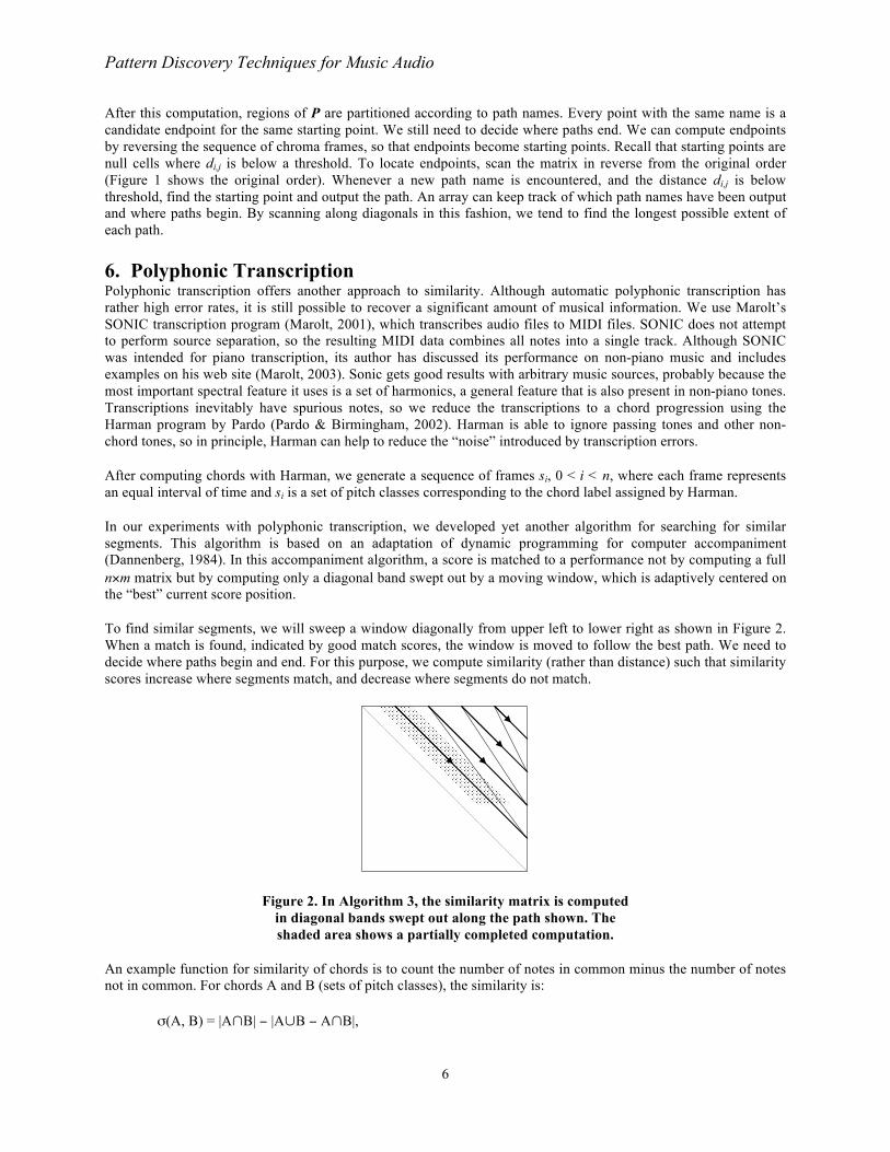
To find similar segments, we will sweep a window diagonally from upper left to lower right as shown in Figure 2. When a match is found, indicated by good match scores, the window is moved to follow the best path. We need to decide where paths begin and end. For this purpose, we compute similarity (rather than distance) such that similarity scores increase where segments match, and decrease where segments do not match.

Figure 2. In Algorithm 3, the similarity matrix is computed in diagonal bands swept out along the path shown. The shaded area shows a partially completed computation.

An example function for similarity of chords is to count the number of notes in common minus the number of notes not in common. For chords A and B (sets of pitch classes), the similarity is:

σ(A, B) = |A∩B| − |A∪B − A∩B|,


7

where |X| is the number of elements in (cardinality of) set X. Other functions were tried, including a count of the number of common pitches, but this has the problem that a dense chord will match almost anything. (A similarity function based on probabilities might work better than our ad hoc approach. This is left for future work.) We will write σi,j to denote σ(si, sj), the similarity between chords at frames i and j.

When we compute the matrix, we initialize cells to zero (again representing null cells) and store only positive values. A path begins when a window element becomes positive and ends when the window becomes zero again. The computation for a matrix cell is:

Mi,j = max(Mi,j−1 − p, Mi−1,j − p, Mi−1,j−1) + σi,j − c

where p is a penalty for insertions and deletions, and c is a bias constant, chosen so that matching segments generate increasing values along the alignment path, and non-matching segments quickly decrease to zero.

The computation of M proceeds as shown by the shaded area in Figure 2. This evaluation order is intended to find locally similar segments and follow their alignment path. The reason for computing in narrow diagonal bands is that if M were computed entire row by entire row, all paths would converge to the main diagonal where all frames match perfectly. At each iteration, cells are computed along one row to the left and right of the current path, spanning data that represents a couple of seconds of time. Because of the limited width of the path, references will be made to null cells in M. These cells and their values are ignored in the maximum value computation.

This algorithm can be further refined. The score along an alignment path will be high at the end of the similar segments, after which the score will decrease to zero. Thus, the algorithm will tend to compute alignment paths that are too long. We can improve on the results by trimming a frame from either end of the path as long as the similarity/length quotient increases. This does not always work well because of local maxima. Another heuristic we use is to trim the final part of a path where the slope is substantially off-diagonal, as shown in Figure 3.

Figure 3. The encircled portion of the alignment path is trimmed because it represents an extreme difference in tempo. The remainder determines a pair of similar segments.

Because the window has a constant size, this algorithm runs in O(n2) time, and by storing only the portion of the matrix swept by the window, O(n) space. The algorithm is quite efficient in practice.

7. Clustering After computing pairs of similar segments with any of the three previously described algorithms, we need to form clusters to identify where segments occur more than twice in the music. For example, if segment A is similar to segment B (as determined by algorithm 1, 2, or 3), and B is similar to C, we expect A to be similar to C, forming the cluster {A, B, C}. Essentially, we are computing the transitive closure of a “similarity” relation over these segments, where “similarity” means either the segments are identified as similar by Algorithm 1, 2, or 3, or the segments overlap significantly. The transitive closure operation produces sets of similar segments, which are the clusters. Our “similarity” relation is not truly transitive, so we may end up with clusters where not every element is “similar” to every other element in the cluster.


8

The algorithm is simple: Start with a set of similar pairs, as computed by Algorithms 1, 2, or 3. For the sake of example, assume the initial set of similar pairs is {(A, B), (B, C), (D, E)}. Remove any pair from the set to form the first cluster. For example, the initial cluster might be the set {A, B}. Then search the set for pairs (a, b) such that either a or b (or both) is an approximate match to a segment in the cluster. If a (or b) is not already in the cluster, add it to the cluster. In the example we would find (B, C), where B is in the cluster {A, B}. Therefore, we add C to the cluster, obtaining {A, B, C}. Continue extending the cluster in this way until all pairs have been examined. (In the example, there are no further additions to the first cluster.) Now, repeat this process to form the next cluster, etc., until the set of pairs is empty. Continuing the example, the final clusters are {A, B, C} and {D, E}.

Recall that segments are defined by their starting times and durations. When clustering actual data, segments will not generally form exact matches. For example, the initial set of pairs might be {(A, B), (B', C), (D, E)}, where B only approximately matches B'. Two segments are considered to be “an approximate match” if their starting times and durations match approximately. We currently require starting times within 10 percent of the duration, and duration matches within 40 percent. These numbers are thought to be reasonable and non-critical, but we have not yet experimented with different values.

Sometimes, a segment in a cluster will correspond to a subsegment of a pair, e.g. the segment (10, 20) overlaps half of the first segment of the pair ((10, 30), (50, 70)). We do not want to add (10, 30) or (50, 70) to the cluster because these have length 20, whereas the cluster element (10, 20) only has length 10. However, it seems clear that there is a segment similar to (10, 20) starting at 50. In this situation, we split the pair proportionally to synthesize a matching pair. In this case, we would create the pair ((10, 20), (50, 60)) and add (50, 60) to the cluster.

8. Analysis as Explanation The final step is to produce an analysis of the musical structure implied by the clusters. We like to view this as an “explanation” process. For each section of music, we “explain” the music in terms of its relationship to other sections. If we could determine relationships of transposition, augmentation, and other forms of variation, these relationships would be part of the explanation. With only similarity, the explanation amounts to labeling music with clusters.

To build an explanation, recall that music is represented by a sequence si, 0 ≤ i < n. Our goal is to fill in an array Ei, 0 ≤ i < n, initially nil, with cluster names, indicating which cluster (if any) contains a note or frame of music. The explanation E serves to describe the music as a structure based on the repetition and organization of patterns.

Recall that a cluster is a set of intervals. For each i in some member of the cluster, we set Ei to the name of the cluster. (Names are arbitrary, e.g. “A”, “B”, “C”, etc.) We then continue searching for the next i such that Ei = nil and i is in some new cluster. We then label additional points in Ei with this new cluster. However, once a label is set, we do not replace it. This gives priority to musical material that is introduced the earliest, which seems to be a reasonable heuristic to resolve conflicts when clusters overlap.

9. Examples We present results from monophonic pitch estimation and chroma-based analyses, and we describe some preliminary results using polyphonic transcription.


9

9.1 Transcription and Algorithm 1 Figure 4 illustrates an analysis of “Naima” using monophonic transcription and Algorithm 1 to find similar segments. Audio is shown at the top to emphasize the input/output relationships for the casual reader. (The authors realize that very little additional information is revealed by these low-resolution waveforms.) Clusters are shown as heavy lines, which show the location of segments, connected by thin lines. The analysis is shown at the bottom of the figure. The simple “textbook” analysis of this piece would be a presentation of the theme with structure AABA, followed by a piano solo. The saxophone returns to play BA followed by a short coda. In the computer analysis, further structure is discovered within the B part (the bridge), indicated in the figure as B1-B1-B2. The transcription failed to detect more than a few notes of the piano solo, but there are a few spurious matching segments here. After the solo, the analysis shows a repetition of the bridge and the A part: B1-B1-B2-A. This is followed by the coda in which there is some repetition. Aside from the solo section, the computer analysis corresponds quite closely to the “textbook” analysis. It can be seen that the A section is half the duration of the B part, which is atypical for an AABA song form. If the program had additional knowledge of standard forms, it might easily guess that this is a slow ballad and uncover additional structure such as the tempo, number of measures, etc. Note, for example, that once the piece is subdivided into segments, further subdivisions are apparent in the RMS amplitude of the audio signal, indicating a duple meter. Additional examples of monophonic analysis are presented in another paper. (Dannenberg & Hu, 2002a)

9.2 Chroma and Algorithm 2 Figure 5 illustrates an analysis of Beethoven’s “Minuet in G” (performed on piano) using the chroma representation and Algorithm 2 for finding similar segments. Because the repetitions are literal and the composition does not involve improvisation, the analysis is definitive, revealing that the structure is: AABBCCDDAB.

Figure 6 applies the same techniques to a pop song (Bagge, Birgisson, & Mumba, 2001) with considerable repetition. Not all of the song structure was recovered because the repetitions are only approximate; however, the analysis shows a structure that is clearly different from the earlier pieces by Coltrane and Beethoven. The repetition was discovered only in sections of audio that are very similar, with identical lyrics and instrumentation. There are

0 2 0 4 0 6 0 8 0 1 0 0 1 2 0 1 4 0 T im e ( s )

Figure 5. Analysis of Beethoven’s Minuet in G performed on piano. The structure, shown at the bottom, is clearly AABBCCDDAB.

A B B’ A A C B A’ A A A A E E A A A A

0 2 0 4 0 6 0 8 0 1 0 0 1 2 0 1 4 0 1 6 0 1 8 0 T im e ( s )

Figure 6. Analysis of a pop song (Samantha Mumba, “Baby Come On Over”). Letters (middle) give a subjective analysis. Bars (bottom) give the machine analysis, showing many repetitions of the A segment. Repetitions of the B and E segments

were not detected, possible because of changes in orchestration and lyrics.


10

some additional musically related sections where the singer is featured and the lyrics are different in each section. Apparently, the changes in lyrics and phrasing give rise to significant differences in the chroma vectors. We would need some other representation that better captures the textural or harmonic similarities in order to discover more musical structure in this example.

9.3 Polyphonic Transcription & Algorithm 3 So far, polyphonic transcription has not yielded good results as anticipated. Recall that we first transcribe a piece of music and then construct a harmonic analysis, so the final representation is a sequence of frames, where each frame is a chord. When we listen to the transcriptions, we can hear the original notes and harmony clearly even though many errors are apparent. Similarly, the harmonic analysis of the transcription seems to retain the harmonic structure of the original music. However, the resulting representation does not seem to have clear patterns that are detectable using Algorithm 3. For example, Algorithm 3 detected 43 pairs of similar segments in Beethoven’s Minuet in G. Many of these represent truly similar segments, but often only fractions, e.g. 5 seconds out of a 15-second repetition. The data contains too many errors to make a successful structural analysis. On the other hand, using synthetic data, Algorithm 3 successfully finds matching segments.

The observed problems are probably due to many factors. The analysis often reports different chords when the music is similar; for example, an A minor chord in one segment and C major in the other. Since these chords have 2 pitch classes in common and 2 that are different, σ(Amin, Cmaj) = 0, whereas σ(Cmaj, Cmaj) = 3. Perhaps there is a better similarity function that gives less penalty for plausible chord substitutions. In addition, chord progressions in tonal music tend to use common tones and are based on the 7-note diatonic scale. This tends to make any two chords chosen at random from a given piece of music more similar, leading to false positives. Sometimes Algorithm 3 identifies two segments that have the same single chord, even though the segments are not otherwise similar. A better similarity metric that requires more context might help here. Also, there is a fine line between similar and dissimilar segments, so finding a good value for the bias constant c is difficult, or perhaps we should use overall length as in Algorithm 2. Finally, the harmonic analysis may be removing useful information along with the “noise.” Overall, the current analysis seems to be too sensitive to small changes in the audio. We believe that we need to alter both the transcriber and the harmonic analysis to achieve a more robust harmonic “summary” of the music information.

To get a better idea of the information content of this representation, Figure 7 is based on an analysis of “Let it Be” performed by the Beatles (McCartney, 1970), using polyphonic analysis and chord labeling. This is the most difficult piece we have studied because the lyrics, instrumentation, and solo lines change with every repetition. After a piano introduction, the vocal melody starts at about 13.5s and finishes the first 4 measures at about 27s. This phrase is repeated throughout the song, so it is interesting to match this known segment against the entire song. Starting at every possible offset, we can search for the best alignment with the score and plot the distance (negative similarity). The distance is zero at 13.5s because the segment matches itself perfectly. The segment repeats almost exactly at about 27s, which appears as a downward spike at 27s. From the graph, it is apparent that the segment also appears with the repetition several other times, as indicated by pairs of downward spikes in the figure.

Correlation With First 4 Bars

0

20

40

60

80

100

120

0 50 100 150 200 250

Time Offset (s)

Dis

tanc

e

Figure 7. The segment from 13.5s to 27s is aligned at every point in the score and the distance is plotted. Downward spikes indicate similar segments, of which there are several.


11

Figure 7 gives a clear indication that the representation contains information and in fact is finding structure within the music; otherwise, the figure would appear random. In this case, we are given the similar segment and only ask “where else does this occur?” We can conclude that the combination of polyphonic transcription followed by harmonic analysis retains significant structural information. Further work is required to use this information to reliably detect similar segments, where the segments are not given a priori.

10. Summary and Conclusions Music audio presents very difficult problems for music analysis and processing because it contains virtually no structure that is immediately accessible to computers. Unless we solve the complete problem of auditory perception and human intelligence, we must consider more focused efforts to derive structure from audio. In this work, we constructed programs that “listen” to music, recognize repeated patterns, and explain the music in terms of these patterns.

Several techniques can be used to derive a music representation that allows similarity comparison. Monophonic transcription works well if the music consists primarily of one monophonic instrument. Chroma is a simplification of the spectrum and applies to polyphonic material. Polyphonic transcription simplified by harmonic analysis offers another, higher-level representation. Three algorithms for efficiently searching for similar patterns were presented. One of these works with note-level representations from monophonic transcriptions and two work with frame-based representations. We demonstrate through examples that the monophonic and chroma analysis techniques recover a significant, and in some cases, essentially complete top-level structure from audio input.

We find it encouraging that these techniques apply to a range of music, including jazz, classical, and popular recordings. Of course, not all music will work as well as our examples. In particular, through-composed music that develops and transforms musical material rather than simply repeating it cannot be analyzed with our systems. This includes improvised jazz and rock soloing, many vocal styles, and most art music. In spite of these difficulties, we believe the premise that listening is based on recognition of repetition and transformation is still valid. The challenge is to recognize repetition and transformation even when it is not so obvious.

Several areas remain for future work. We are working to better understand the polyphonic transcription data and harmonic analysis, which offer great promise for finding similarity in the face of musical variations. We believe the analysis can be made less sensitive to small variations in audio, resulting in a better “harmonic summary” and leading to more successful structural analysis. In the work described here, we built several independent systems and tested them with (mostly) different musical examples, so it is hard to attribute success or failure to specific components (the features from signal analysis, the similarity algorithms, parameter settings, and the music example). In general, when analyses fail, we are unable to make much improvement simply by adjusting parameters, and we did not use different parameter settings for the results described here. Although we are continuing work to resolve some basic questions and better understand our results, we think it is even more important to develop more formal models of structure and similarity. For example, a model could enable us to search for patterns and clusters that give the “best” global explanation for observed similarities. The distance metrics used for finding similar segments could also use a more formal approach. Distance metrics should reflect the probability that two segments are not similar. A formal model of structure might help us to be more precise about assumptions made in our work, important characteristics of music signals for analysis, and requirements of various representations to achieve success in music analysis.

Another enhancement to our work would be the use of hierarchy in explanations. This would, for example, support a two-level explanation of the bridge in “Naima.” It would be interesting to combine data from beat tracking, key analysis, and other techniques to obtain a more accurate view of music structure. A reviewer also suggested the interesting possibility of using Algorithms 1, 2, and 3 in combination rather than as alternatives. Finally, it would be interesting to find relationships other than repetition. Transposition of small phrases is a common relationship within melodies, but we do not presently detect anything other than repetition. Transposition often occurs in very short sequences, so a good model of musical sequence comparison that incorporates rhythm, harmony, and pitch seems to be necessary to separate random matches from intentional ones.

In conclusion, we offer a set of new techniques and our experience using them to analyze music audio, obtaining structural descriptions. These descriptions are based entirely on the music and its internal structure of similar


12

patterns. Our results suggest this approach is promising for a variety of music processing tasks, including music search, where programs must derive high-level structures and features directly from audio representations.

Acknowledgments This work was supported by the National Science Foundation under award number 0085945. Ann Lewis assisted in the preparation and processing of data. Matija Marolt offered the use of his SONIC transcription software, which enabled us to explore the use of polyphonic transcription for music analysis. Mark Bartsch and Greg Wakefield provided chroma analysis software. We would also like to thank Bryan Pardo for his Harman program and assistance using it. Finally, we thank our other colleagues at the University of Michigan for their collaboration and many stimulating conversations.

References Altschul, S. F., Gish, W., Miller, W., Myers, E. W., & Lipman, D. J. (1990). "A Basic Local Alignment Search

Tool." Journal of Molecular Biology, 215, 403-410.

Aucouturier, J.-J., & Sandler, M. (2001). Segmentation of Musical Signals Using Hidden Markov Models. Proceedings of the 110th Audio Engineering Society Convention. AES.

Aucouturier, J.-J., & Sandler, M. (2002). Finding Repeating Patterns in Acoustic Musical Signals: Applications for Audio Thumbnailing. AES22 International Conference on Virtual, Synthetic and Entertainment Audio (pp. 412-421). Audio Engineering Society.

Bagge, A., Birgisson, A., & Mumba, S. (2001). Baby Come On Over, Baby Come On Over (CD Single): Polydor.

Bartsch, M., & Wakefield, G. H. (2001). To Catch a Chorus: Using Chroma-Based Representations For Audio Thumbnailing. Proceedings of the Workshop on Applications of Signal Processing to Audio and Acoustics. IEEE.

Birmingham, W. P., Dannenberg, R. B., Wakefield, G. H., Bartsch, M., Bykowski, D., Mazzoni, D., Meek, C., Mellody, M., & Rand, W. (2001). MUSART: Music Retrieval Via Aural Queries. International Symposium on Music Information Retrieval (pp. 73-81).

Brown, J. (1999). "Computer Identification of Musical Instruments." Journal of the Acoustical Society of America, 105(3), 1933-1941.

Coltrane, J. (1960). Naima, Giant Steps: Atlantic Records.

Conklin, D., & Anagnostopoulou, C. (2001). Representation and Discovery of Multiple Viewpoint Patterns. Proceedings of the 2001 International Computer Music Conference (pp. 479-485). San Francisco: International Computer Music Association.

Cope, D. (1996). Experiments in Musical Intelligence (Vol. 12). Madison, Wisconsin: A-R Editions, Inc.

Dannenberg, R. B. (1984). An On-Line Algorithm for Real-Time Accompaniment. Proceedings of the 1984 International Computer Music Conference (pp. 193-198). San Francisco: International Computer Music Association. (http://www.cs.cmu.edu/~rbd/bib-accomp.html#icmc84)

Dannenberg, R. B. (2002). Listening to "Naima": An Automated Structural Analysis from Recorded Audio. Proceedings of the 2002 International Computer Music Conference (pp. 28-34). San Francisco: International Computer Music Association.

Dannenberg, R. B., & Hu, N. (2002a). Discovering Musical Structure in Audio Recordings. In C. Anagnostopoulou,M. Ferrand & A. Smaill (Eds.), Music and Artificial Intelligence, Second International Conference, ICMAI 2002 (pp. 43-57). Berlin: Springer-Verlag.

Dannenberg, R. B., & Hu, N. (2002b). Pattern Discovery Techniques for Music Audio. ISMIR 2002 Conference Proceedings (pp. 63-70). IRCAM.

Dixon, S. (2000). A Lightweight Multi-agent Musical Beat Tracking System. Proceedings of the Pacific Rim International Conference on Artificial Intelligence (pp. 778-788).


13

Fingerhut, M. (Ed.). (2002). ISMIR 2002 Conference Proceedings. Paris: IRCAM.

Foote, J., & Cooper, M. (2001). Visualizing Musical Structure and Rhythm via Self-Similarity. Proceedings of the 2001 International Computer Music Conference (pp. 419-422). International Computer Music Association.

Fujinaga, I. (2000). Realtime Recognition of Orchestral Instruments. Proceedings of the 2000 International Computer Music Conference (ICMC) (pp. 141-143). International Computer Music Association.

Fujishima, T. (1999). Realtime Chord Recognition of Musical Sound: a System Using Common Lisp Music. Proceedings of the 1999 International Computer Music Conference (pp. 464-467). San Francisco: International Computer Music Association.

Goto, M. (2001). A Predominant-F0 Estimation Method for CD Recordings: MAP Estimation using EM Algorithm for Adaptive Tone Models. 2001 IEEE International Conference on Acoustics, Speech, and Signal Processing (pp. V-3365-3368). IEEE.

Goto, M., & Muraoka, Y. (1998). Music Understanding at the Beat Level: Real-Time Beat Tracking of Audio Signals. In D. Rosenthal & H. Okuno (Eds.), Computational Auditory Scene Analysis. New Jersey: Lawrence Erlbaum Associates.

Hewlett, W., & Selfridge-Field, E. (Eds.). (1998). Melodic Similarity: Concepts, Procedures, and Applications (Vol. 11). Cambridge: MIT Press.

Hu, N., & Dannenberg, R. B. (2002). A Comparison of Melodic Database Retrieval Techniques Using Sung Queries. Joint Conference on Digital Libraries. Association for Computing Machinery.

Klapuri, A. (1998). Automatic Transcription of Music. M.Sc. Thesis, Tampere University of Technology, Finland. (http://www.cs.tut.fi/~klap/iiro/contents.html)

Lartillot, O., Dubnov, S., Assayag, G., & Bejerano, G. (2001). Automatic Modeling of Musical Style. Proceedings of the 2001 International Computer Music Conference (pp. 447-454). San Francisco: International Computer Music Association.

Marolt, M. (2001). SONIC: Transcription of Polyphonic Piano Music With Neural Networks. Workshop on Current Research Directions in Computer Music (pp. 217-224). Barcelona, Spain: Audiovisual Institute, Pompeu Fabra University.

Marolt, M. (2003). SONIC: Transcription of Polyphonic Piano Music. (web page). http:// http://lgm.fri.uni-lj.si/~matic/SONIC.html.

McCartney, P. (1970). Let It Be, Let It Be: Apple Records.

Meek, C., & Birmingham, W. P. (2001). Thematic Extractor. 2nd Annual International Symposium on Music Information Retrieval (pp. 119-128). Bloomington: Indiana University.

Mongeau, M., & Sankoff, D. (1990). Comparison of Musical Sequences. In W. Hewlett & E. Selfridge-Field (Eds.), Melodic Similarity Concepts, Procedures, and Applications (Vol. 11). Cambridge: MIT Press.

Mont-Reynaud, B., & Goldstein, M. (1985). On Finding Rhythmic Patterns in Musical Lines. Proceedings of the International Computer Music Conference 1985 (pp. 391-397). San Francisco: International Computer Music Association.

Narmour, E. (2000). "Music Expectation by Cognitive Rule-Mapping." Music Perception, 17(3), 329-398.

Ottaviani, L., & Rocchesso, D. (2001). Separation of Speech Signal from Complex Auditory Scenes. Proceedings of the COST G-6 Conference on Digital Audio Effects (DAFX). (http://www.csis.ul.ie/dafx01/proceedings/navig/toc.htm)

Pardo, B., & Birmingham, W. P. (2002). "Algorithms for Chordal Analysis." Computer Music Journal, 26(2), 27-49.

Pearson, W. R. (1990). "Rapid and Sensitive Sequence Comparison with FASTP and FASTA." Methods in Enzymology, 183, 63-98.


14

Roads, C. (1996). Autocorrelation Pitch Detection, The Computer Music Tutorial (pp. 509-511). Cambridge: MIT Press.

Rolland, P.-Y., & Ganascia, J.-G. (2000). Musical pattern extraction and similarity assessment. In E. Miranda (Ed.), Readings in Music and Artificial Intelligence (pp. 115-144). New York: Harwood Academic Publishers.

Sankoff, D., & Kruskal, J. B. (1983). Time Warps, String Edits, and Macromolecules: The Theory and Practice of Sequence Comparison. Reading, MA: Addison-Wesley.

Sapp, C. S. (2001). Harmonic Visualization of Tonal Music. Proceedings of the 2001 International Computer Music Conference (pp. 423-430). San Francisco: International Computer Music Association.

Simon, H. A., & Sumner, R. K. (1968). Pattern in Music. In B. Kleinmuntz (Ed.), Formal Representation of Human Judgment. New York: Wiley. Reprinted in S. Schwanauer and D. Levitt, eds., Machine Models of Music, MIT Press, pp. 83-112.

Slaney, M. (1998). Auditory Toolbox. Palo Alto: Interval Research Corporation. (http://rvl4.ecn.purdue.edu/~malcolm/interval/1998-010/)

Smith, T. F., & Waterman, M. S. (1981). "Identification of Common Molecular Subsequences." Journal of Molecular Biology, 147(1), 195-197.

Stammen, D., & Pennycook, B. (1993). Real-Time Recognition of Melodic Fragments Using the Dynamic Timewarp Algorithm. Proceedings of the 1993 International Computer Music Conference (pp. 232-235). San Francisco: International Computer Music Association.

Yli-Harja, O., Shmulevich, I., & Lemstrom, K. (1999). Graph-based Smoothing of Class Data with Applications in Musical Key Finding. Proceedings of IEEE-EURASIP Workshop on Nonlinear Signal and Image Processing. IEEE.

FOOTNOTES

1 To understand why, assume there are similar segments, ((i, k), (j, l)), that overlap, i.e. 0 ≤ i < j ≤ k < l < n. Then, there is some subsegment of (i, k) we will call (i, m) , m < k, corresponding to the overlapping region (j, k) and some subsegment of (k, l) we will call (p, l), p > j, corresponding to (j, k). Thus, there are three similar segments (i, m), (j, k), and (p, l) that provide an alternate structure to the original overlapping pair. In general, a shorter, more frequent pattern is preferable, so we do not search for overlapping patterns.

2 An implementation note: for each pair of similar segments, the starting points are implied by the coordinates i, j, but we need to store durations. Since we only search half of the matrix due to symmetry, we store one duration at location i, j and the other at j, i.

pattern discovery techniques for music audio./rbd/papers/patterndiscovery-jnmr-web.pdf · pattern...

Documents