FuncICA for time series pattern discovery

Nishant Mehta and Alexander Gray

Georgia Institute of Technology

The problem

Given a set of inherently continuous time series (e.g. EEG)

Find a set of patterns that vary independently over the data

Existing solutions:

1 Standard independent component analysis (ICA)

2 Functional principal component analysis

2 / 29

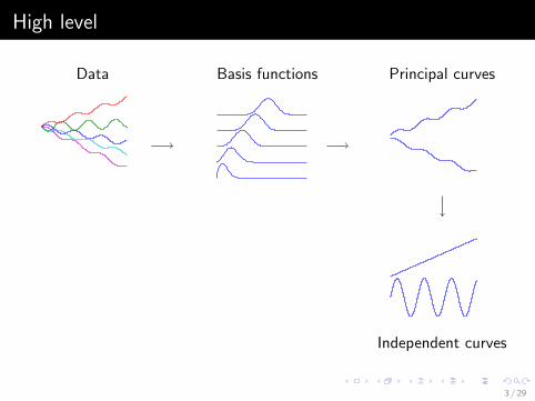
High level

Data Basis functions Principal curves

Independent curves

3 / 29

High level

FuncICA - Functional independent component analysis

• ICA for time series data

1 Express the data using a set of basis functions.

2 Functional PCA - Find the k curves of maximum variation across thedata, subject to smoothness constraint

3 Rotate functional principal components to maximize independence andyield independent components Y

4 Optimize an independence objective Q(Y ) with respect to asmoothness regularization term

4 / 29

Towards automating science

• ICA used in pattern discovery in natural domains like neuroscience,genetics, and astrophysics, but patterns are often smooth

• Many domains created by humans, including financial markets andchemical processes, involve smooth variation

• FuncICA offers a way to find optimally smoothed patterns in thesedomains.

• Automatic identification of event-related potentials in EEG• Automatic discovery of gene signaling mechanisms from microarray

gene expression data• Identifying spatiotemporal activation patterns in fMRI

5 / 29

Independent component analysis

• Observe multiple signals X (t) over time

• Univariate signal X(t)i is mixture of independent sources S (t)

• Linear instantaneous mixing model: X (t) = AS (t)

• Find unmixing transformation that maximizes statistical independenceof recovered sources

Sources Mixtures

0 5 10 15 20 25 30 35−1

−0.5

0

0.5

1

0 5 10 15 20 25 30 35−0.4

−0.2

0

0.2

0.4

0.6

0 5 10 15 20 25 30 35−0.5

0

0.5

1

0 5 10 15 20 25 30 35−0.4

−0.2

0

0.2

0.4

0.6

6 / 29

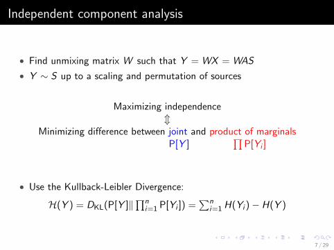
Independent component analysis

• Find unmixing matrix W such that Y = WX = WAS

• Y ∼ S up to a scaling and permutation of sources

Maximizing independencem

Minimizing difference between joint and product of marginalsP[Y ]

∏P[Yi ]

• Use the Kullback-Leibler Divergence:

H(Y ) = DKL(P[Y ]‖∏ni=1 P[Yi ]) =

∑ni=1 H(Yi )− H(Y )

7 / 29

ICA duality

Primal Dual

IC1 varies in loading over samples of x

x1

x2

sample 1

IC1

IC1 loadingvaries oversamples

sample 1

sample 2

〈sample 1

,

IC1

〉

8 / 29

Why functional data?

• Higher sampling rate ⇒ Higher dimensional data• No principled way of dimensionality reduction

• Subsampling?

• No principled way to handle asynchronous observations• Missing data from occasionally offline sensors• Each observation lives in different space

• Alternative?Generative (parametric) models - HMM, dynamic Bayesian network

ORFunctional representation

9 / 29

Functional data

• Set of n curves X = {X1(t), . . . ,Xn(t)},Xi ∈ X• Set of m basis functions β = {β1, . . . , βm}• Decompose data as Xi (t) =

∑mj=1 ψi ,jβj(t)

• X ⊂ L2 (Hilbert space), with inner product 〈f , g〉 =∫

f (t)g(t)dt

0 0.1 0.2 0.3 0.4 0.5 0.6 0.7 0.8 0.9 10

0.1

0.2

0.3

0.4

0.5

0.6

0.7

13

15

17

10 / 29

Functional PCA

Functional PCA to get principal curves

Ei (t) =m∑

j=1

ρi ,jβj(t)

Principal components (curve loadings) over the data

σ(E)i ,j = 〈Ei ,Xj〉 =

m∑k=1

m∑l=1

ρi ,k〈βk , βl〉ψj ,l

σ(E) = ρBψT

11 / 29

Functional ICA

Independent curves are rotation W of principal curves

Yi (t) =m∑

j=1

[W ρ]i ,jβj(t)

Independent components

σ(Y )i ,j = 〈Yi ,Xj〉 =

m∑k=1

m∑l=1

[W ρ]i ,k〈βk , βl〉ψj ,l

σ(Y )= Wσ(E)

Now, just solve for W to find IC basis weights φ = W ρ

12 / 29

Independence objective

KL-divergence objective

H(Y ) =n∑

i=1

H(Yi )− H(Y )

After FPCA, we have

H(E ) =n∑

i=1

H(Ei )− H(E )

Y = WE and W orthogonal yield minimum marginal entropy objective

H∗(Y ) =n∑

i=1

H(Yi )

13 / 29

Entropy estimator to evaluate H(Yi)

Vasicek entropy estimator

• nonparametric entropy estimator that considers order statistics

1 Order samples in non-decreasing order Z (1) ≤ Z (2) . . . ≤ Z (N)

2 m-spacing is Z (i+m) − Z (i)

3 HN(Z 1,Z 2, . . . ,ZN) =

1

N

N−mN∑i=1

log

(N

mN(Z (i+mN) − Z (i)

)

14 / 29

Optimizer

Plug-in ICA estimator: RADICAL ICA[Learned-Miller and Fisher 2003]

• RADICAL uses Vasicek entropy estimator

• For ICA in D dimensions (D eigenfunctions), do pairwise separation.

• 2-D rotation matrix is parameterized by one angle parameter θ:(cos θ sin θ− sin θ cos θ

)Since θ ∈ [−π

2 ,π2 ], use brute-force to optimize HN(θ)

15 / 29

Smoothing

• FPCA chooses smoothing level α∗p minimizing leave-one-outcross-validation error

• α∗p not optimal for source recovery

• FuncICA balances reconstruction error while avoiding Gaussiancomponents

16 / 29

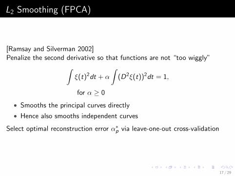
L2 Smoothing (FPCA)

[Ramsay and Silverman 2002]Penalize the second derivative so that functions are not “too wiggly”∫

ξ(t)2dt + α

∫(D2ξ(t))2dt = 1,

for α ≥ 0

• Smooths the principal curves directly

• Hence also smooths independent curves

Select optimal reconstruction error α∗p via leave-one-out cross-validation

17 / 29

Inverse negentropy smoothing (FuncICA)

Motivation - Penalize Gaussian componentsWhy?

• ICA fails if there is more than 1 Gaussian component

• Oversmoothing ⇒ components become noisy ⇒ non-Gaussiancomponents may become Gaussian

How? Inverse negentropy objective function:

Q(Y ) =

p∑i=1

1

J(Yi )

where J(Yi ) = H(N (0, 1))− H(Yi ) is the negentropy of unit-variance Yi

18 / 29

Optimal FuncICA inverse negentropy smoothing

Algorithm

1 α = α∗p, τ = 0, Q(0) =∞2 repeat

3 τ = τ + 1

4 (Y ,Q(τ)) = FuncICA(X , α(τ))

5 α(τ+1) = γα(τ)

6 until Q(τ) > Q(τ−1)

7 return α(τ−1)

Intuition:

• α∗p optimally smooths for reconstruction error

• Can further smoothing be beneficial for source recovery?

Yes! Can effectively dampen Gaussian noise components

19 / 29

Synthetic data results

• Perfect source recovery for mixtureof Laplace-distributed harmonics

0 0.1 0.2 0.3 0.4 0.5 0.6 0.7 0.8 0.9 1−2

−1.5

−1

−0.5

0

0.5

1

1.5

2

t

f(t)

• Successful isolation of single high-frequency Gaussian source• FuncICA performs well for α ≥ 0• FPCA blends high-frequency source into all recovered curves

• Dampening of two high-frequency Gaussian sources• Q statistic performs well in recovering Laplacian sources

20 / 29

Synthetic data results

Source curves DistributionsS1(t) = 1√

2sin(10πt) ← Laplace

S2(t) = 1√2

cos(10πt) ← Laplace

S3(t) = sin(40πt) ← GaussianS4(t) = cos(40πt) ← Gaussian

10−10 10−9 10−895

100

105

110

115

120

125

130Effect of smoothing on Q

α

Q

10−10 10−9 10−80.988

0.99

0.992

0.994

0.996

0.998

1

1.002Effect of smoothing on accuracy

α

accu

racy

21 / 29

Event-related potential discovery results

column row letter0

0.1

0.2

0.3

0.4

0.5

0.6

0.7A

ccur

acy

FuncICAICAFPCAEmpirical P300

22 / 29

Microarray gene expression results

• 6178 genes observed at 18 times in7 minute increments

• Goal: identify co-regulated genesrelated to specific phases of the cellcycle

• G1 phase regulated vs non-G1

phase regulated

IC PC

Top 11 7.1% 9.2%

Filtered 6.2% 8.2%

23 / 29

Conclusion

• Functional ICA offers a way to find smooth, independent modes ofvariation in time series and other continuous-natured data

• Alternative to FPCA when components of interest may not beGaussian

• Applicable for EEG, gene expression, finance, and other domains

24 / 29

Questions?

25 / 29

Perhaps not functional PCA

Let’s see what FPCA does for our ERP data

0 0.1 0.2 0.3 0.4 0.5 0.6 0.7 0.8 0.9 1−2

−1.5

−1

−0.5

0

0.5

1

1.5

2

t

f(t)

Looks like a Fourier basisMakes sense

• α rhythm

• β rhythm

• µ rhythm

26 / 29

Let’s see what Functional ICA (FuncICA) extracts

0 0.1 0.2 0.3 0.4 0.5 0.6 0.7 0.8 0.9 1−3

−2

−1

0

1

2

3IC closest to P300 ERP for α = 5E−8

t

IC6(t)

0 0.1 0.2 0.3 0.4 0.5 0.6 0.7 0.8 0.9 10.5

1

1.5

2

2.5

3

3.5Empirical P300 waveform

t

P300

(t)

0 0.1 0.2 0.3 0.4 0.5 0.6 0.7 0.8 0.9 1−2.5

−2

−1.5

−1

−0.5

0

0.5

1

1.5

2IC closest to P300 ERP for α = 1E−7

t

IC3(t)

Closest IC to P300 for α = 5 · 10−5

Empirical P300 waveform calculatedfrom 2550 trials

Closest IC to P300 for α = 1 · 10−7

27 / 29

Event-related potential discovery results

10−8

10−7

10−6

750

800

850

900

950

1000

1050

1100

1150

1200

1250Effect of smoothing on Q

α

Q

10−8

10−7

10−6

0.44

0.46

0.48

0.5

0.52

0.54

0.56

0.58

0.6Effect of smoothing on accuracy

α

accu

racy

28 / 29

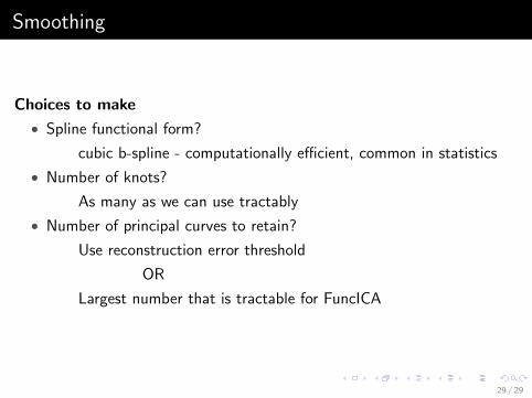
Smoothing

Choices to make

• Spline functional form?

cubic b-spline - computationally efficient, common in statistics

• Number of knots?

As many as we can use tractably

• Number of principal curves to retain?

Use reconstruction error threshold

OR

Largest number that is tractable for FuncICA

29 / 29