Energy Procedia 59 ( 2014 ) 90 – 96

Available online at www.sciencedirect.com

ScienceDirect

1876-6102 © 2014 The Authors. Published by Elsevier Ltd. This is an open access article under the CC BY-NC-ND license (http://creativecommons.org/licenses/by-nc-nd/3.0/).Peer-review under responsibility of the Austrian Academy of Sciencesdoi: 10.1016/j.egypro.2014.10.353

European Geosciences Union General Assembly 2014, EGU 2014

Passive seismic ambient noise correlation: an example from the Ketzin experimental CO2 storage site, GermanyFengjiao Zhanga,b*, Christopher Juhlinb, and Daniel Sopherb

aJilin University, Changchun 130026, ChinabDepartment of Earth Sciences, Uppsala University, Uppsala 75236, Sweden

Abstract

Passive seismic ambient noise correlation is potentially a new tool to monitor carbon dioxide storage sites. Unlike conventional monitoring tools, such as time-lapse active seismic surveys, the passive seismic ambient noise correlation method is a relatively low cost method and can be performed together with microseismic and reservoir monitoring. In this study, we test the method atthe Ketzin CO2 storage site, Germany. A new passive seismic survey was performed in August 2013 together with an active

geophones spaced at 24 m intervals and Line 2 contained 23 DSU3 (3-component MEMS) sensors spaced at 5 m intervals. In total, 6 nights and 3 daytime series of ambient noise data were recorded. First, we applied autocorrelation to the passive data records to reconstruct the e results show good structural correlation with a stacked section from the active data. Then we used passive seismic interferometry to reconstruct common shot gathers for each receiver location. Surface waveswere observed in some retrieved gathers from Line 1. However, for Line 2 we also observed refracted and reflected waves in some retrieved shot gathers. Here we review ambient noise correlation methods and compare our results with active seismic data.

© 2014 The Authors. Published by Elsevier Ltd.Peer-review under responsibility of the Austrian Academy of Sciences.

Keywords: CO2 storage; seismic interferometry; microseismic; ambient noise correlation

* Corresponding author. Tel.: +46-73-9961089; fax: +46-18-501110.E-mail address: fengjiao.zhang@geo.uu.se

© 2014 The Authors. Published by Elsevier Ltd. This is an open access article under the CC BY-NC-ND license (http://creativecommons.org/licenses/by-nc-nd/3.0/).Peer-review under responsibility of the Austrian Academy of Sciences

Fengjiao Zhang et al. / Energy Procedia 59 ( 2014 ) 90 – 96 91

1. Introduction

The Ketzin pilot site is the EU's first experimental onshore CO2 injection site and is located in Ketzin, west of Berlin, Germany. The injection started in June 2008 and ended in August 2013 with about 67000 tons of CO2 having been injected into the reservoir. An extensive time-lapse seismic monitoring program has been performed at the Ketzin site. The monitoring program includes full and sparse 3D time-lapse reflection seismic surveys [1,2,3], 2D time-lapse reflection seismic surveys [3], time-lapse borehole seismic surveys (crosshole and moving source profiling), vertical seismic profiling [4] and microseismic surveys. These conventional seismic monitoring tools are usually quite expensive to perform. Passive seismic ambient noise correlation is a relatively low cost method and can be performed together with microseismic and reservoir monitoring. These advantages make it a new potential tool to monitor carbon dioxide storage sites. A previous passive seismic survey was performed in 2011 to test this method at the Ketzin site [5]. In this study, we acquired a new passive seismic survey to further test the method.

interferometry was used to reconstruct common shot gathers for each receiver location. The active data set was also processed for comparison.

The new passive seismic survey was performed in August 2013. At the same time an active survey along line 1

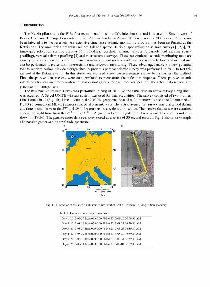
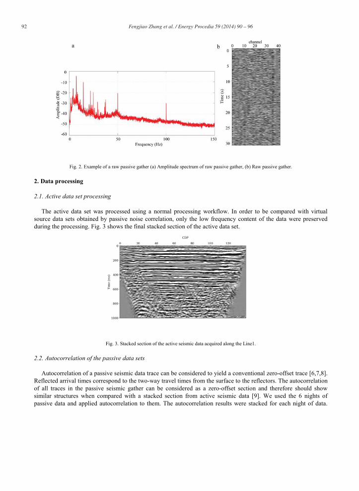
Line 1 and Line 2 (Fig. 1b). Line 1 contained 42 10 Hz geophones spaced at 24 m intervals and Line 2 contained 23 DSU3 (3 component MEMS) sensors spaced at 5 m intervals. The active source test survey was performed during day time hours, between the 27th and 29th of August using a weight drop source. The passive data sets were acquired during the night time from the 25th to the 31st of August. In total, 6 nights of ambient noise data were recorded as shown in Table1. The passive noise data sets were stored as a series of 30 second records. Fig. 2 shows an example of a passive gather and its amplitude spectrum.

Fig. 1. (a) Location of the Ketzin CO2 storage site, west of Berlin, Germany, (b) Acquisition geometry.

Table 1. Passive seismic acquisition details.

Day 1: 2013-08-25 from 08:00:00 PM to 2013-08-26 06:59:30 AM

Day 2: 2013-08-26 from 07:00:00 PM to 2013-08-27 06:59:30 AM

Day 3: 2013-08-27 from 07:00:00 PM to 2013-08-28 06:59:30 AM

Day 4: 2013-08-29 from 07:00:00 PM to 2013-08-30 06:59:30 AM

Day 5: 2013-08-30 from 07:00:00 PM to 2013-08-31 06:59:30 AM

Day 6: 2013-08-31 from 07:00:00 PM to 2013-09-01 06:59:30 AM

92 Fengjiao Zhang et al. / Energy Procedia 59 ( 2014 ) 90 – 96

Fig. 2. Example of a raw passive gather (a) Amplitude spectrum of raw passive gather, (b) Raw passive gather.

2. Data processing

2.1. Active data set processing

The active data set was processed using a normal processing workflow. In order to be compared with virtual source data sets obtained by passive noise correlation, only the low frequency content of the data were preserved during the processing. Fig. 3 shows the final stacked section of the active data set.

Fig. 3. Stacked section of the active seismic data acquired along the Line1.

2.2. Autocorrelation of the passive data sets

Autocorrelation of a passive seismic data trace can be considered to yield a conventional zero-offset trace [6,7,8]. Reflected arrival times correspond to the two-way travel times from the surface to the reflectors. The autocorrelation of all traces in the passive seismic gather can be considered as a zero-offset section and therefore should show similar structures when compared with a stacked section from active seismic data [9]. We used the 6 nights of passive data and applied autocorrelation to them. The autocorrelation results were stacked for each night of data.

Fengjiao Zhang et al. / Energy Procedia 59 ( 2014 ) 90 – 96 93

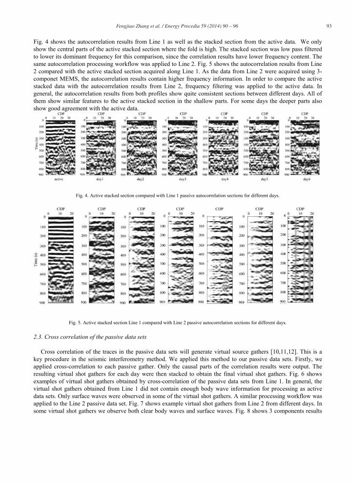
Fig. 4 shows the autocorrelation results from Line 1 as well as the stacked section from the active data. We only show the central parts of the active stacked section where the fold is high. The stacked section was low pass filtered to lower its dominant frequency for this comparison, since the correlation results have lower frequency content. The same autocorrelation processing workflow was applied to Line 2. Fig. 5 shows the autocorrelation results from Line 2 compared with the active stacked section acquired along Line 1. As the data from Line 2 were acquired using 3-componet MEMS, the autocorrelation results contain higher frequency information. In order to compare the active stacked data with the autocorrelation results from Line 2, frequency filtering was applied to the active data. In general, the autocorrelation results from both profiles show quite consistent sections between different days. All of them show similar features to the active stacked section in the shallow parts. For some days the deeper parts also show good agreement with the active data.

Fig. 4. Active stacked section compared with Line 1 passive autocorrelation sections for different days.

Fig. 5. Active stacked section Line 1 compared with Line 2 passive autocorrelation sections for different days.

2.3. Cross correlation of the passive data sets

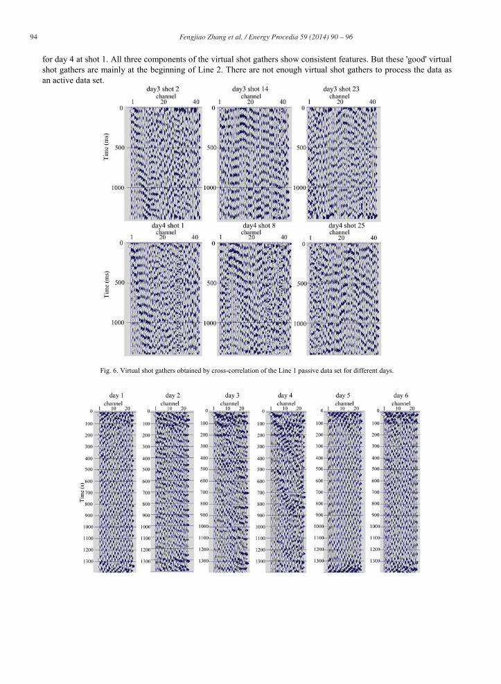
Cross correlation of the traces in the passive data sets will generate virtual source gathers [10,11,12]. This is a key procedure in the seismic interferometry method. We applied this method to our passive data sets. Firstly, we applied cross-correlation to each passive gather. Only the causal parts of the correlation results were output. The resulting virtual shot gathers for each day were then stacked to obtain the final virtual shot gathers. Fig. 6 shows examples of virtual shot gathers obtained by cross-correlation of the passive data sets from Line 1. In general, the virtual shot gathers obtained from Line 1 did not contain enough body wave information for processing as active data sets. Only surface waves were observed in some of the virtual shot gathers. A similar processing workflow was applied to the Line 2 passive data set. Fig. 7 shows example virtual shot gathers from Line 2 from different days. In some virtual shot gathers we observe both clear body waves and surface waves. Fig. 8 shows 3 components results

94 Fengjiao Zhang et al. / Energy Procedia 59 ( 2014 ) 90 – 96

for day 4 at shot 1. All three components of the virtual shot gathers show consistent features. But these 'good' virtual shot gathers are mainly at the beginning of Line 2. There are not enough virtual shot gathers to process the data as an active data set.

Fig. 6. Virtual shot gathers obtained by cross-correlation of the Line 1 passive data set for different days.

Fengjiao Zhang et al. / Energy Procedia 59 ( 2014 ) 90 – 96 95

Fig. 7. Virtual shot gathers obtained by cross-correlation of the Line 2 passive data set for different days.

Fig. 8. Virtual shot gathers obtained by cross-correlation of the Line 2 passive data set, day 4 of shot 1 for different components.

3. Conclusion

Autocorrelation of Line 1 and Line 2 provides reasonable results compared with the active stacked section, showing good structural correlation with it. The cross-correlation results from Line 1 did not provide enough good quality virtual shot gathers for processing them as active data. Only some surface waves were observed in day 3 and day 4. Cross-correlation of Line 2 gives better results compared with Line 1. Some shot gathers at the beginning of Line 2 (mostly from day 3 and day 4, first 7 to 8 of 23 locations) show both body waves and surface waves. The seismic interferometry method sometimes generates good virtual shot gathers, but the results are highly variable. Although, the passive seismic ambient noise correlation method has many drawbacks, it still could potentially be used as a passive monitoring tool for CO2 injection when large amounts of CO2 are injected.

Acknowledgements

The Swedish Research Council (VR) partly funded Daniel Sopher during this research (project number 2010-3657) and is gratefully acknowledged. Seismic data acquisition was partly funded by the Geotechnologien program of the German Federal Ministry of Education and Research. GLOBE ClaritasTM under license from the Institute of Geological and Nuclear Sciences, Limited, Lower Hutt, New Zealand was used to process the seismic data.

References

[1] Juhlin C, Giese R, Zinck-Jørgensen K, Cosma C, Kazemeini H, Juhojuntti N, Lüth S, Norden B, Förster A. 3D baseline seismics at Ketzin, Germany: the CO2SINK project. Geophys 2007; 72:B121–B132.

[2] Ivandic M, Yang C, Lüth S, Cosma C, Juhlin C. Time-lapse analysis of sparse 3D seismic data from the CO2 storage pilot site at Ketzin, Germany. J Appl Geophys 2012; 84:14-28.

[3] Ivandic M, Juhlin C, Lüth S, Bergmann P, Kashubin A. Geophysical monitoring of CO2 at the Ketzin storage site - the results of the second 3D repeat seismic survey. 75th EAGE Conference & Exhibition Incorporating SPE EUROPEC 2013.

96 Fengjiao Zhang et al. / Energy Procedia 59 ( 2014 ) 90 – 96

[4] Yang C. Time-lapse analysis of borehole and surface seismic data, and reservoir characterization of the Ketzin CO2 storage site, Germany. Ph.D. Dissertation, Uppsala University; 2012.

[5] Xu Z, Juhlin C, Gudmundsson O, Zhang F, Yang C, Kashubin A, Lüth S. Reconstruction of subsurface structure from ambient seismic noise: an example from Ketzin, Germany. Geophys J Int 2012; 189: 1085–1102.

[6] Aki K. Space and time spectra of stationary stochastic waves with special reference to microtremors. Bull Earthquake Res Inst 1957; 35: 415-456.

[7] Ridder S, Biondi B. Low frequency passive seismic interferometry for land data. 80th Annual International Meeting, SEG, Expanded Abstracts 2010; 29: 4041-4046.

[8] Draganov D, Campman X, Thorbecke J, Verde A, Wapenaar K. Reflection images from ambient seismic noise. Geophys 2009; 74: A63.[9] Edme P, Halliday. Extracting Reflectivity Response From Point-receiver Ambient Noise. SEG Technical Program Expanded Abstracts

2011;1602-1607.[10] Bakulin A, Calvert R. The virtual source method: Theory and case study. Geophys 2006; 71:S1139-s1150.[11] Wapenaar K, Draganov D, Snieder R, Campman X, Verdel A. Tutorial on seismic interferometry: Part 1 – Basic principles and application.

Geophys 2010; 75:A195-A209.[12] Wapenaar K, Slob E, Snieder R, Curtis A. Tutorial on seismic interferometry: Part 2 – Underlying theory and new advances. Geophys 2010;

75:A211-A227.