1 correlation of seismic attributes and geo-mechanical...
TRANSCRIPT

1
Correlation of seismic attributes and geo-mechanical properties to the rate of penetration in the 1
Mississippian Limestone, Oklahoma 2
Xuan Qi, Joseph Snyder, Tao Zhao, Kurt J. Marfurt, and Matthew J. Pranter1 3
ConocoPhillips school of Geology and Geophysics, University of Oklahoma, USA 4
100 E. Boyd St., Norman, Oklahoma, 73019 5
11
12

2
Acknowledgement 13
We thank the sponsors of the “Mississippi Lime” and Attribute Assisted Seismic 14
Processing & Interpretation (AASPI) Consortia at the University of Oklahoma: Anadarko, Arcis, 15
BGP, BHP Billiton, Lumina Geophysical, Chesapeake Energy, Chevron, ConocoPhillips, Devon 16
Energy, EnerVest, ExxonMobil, Geophysical Insights, Institute of Petroleum, Marathon Oil, 17
Newfield Exploration, Occidental Petroleum, Petrobras, Pioneer Natural Resources, QEP, 18
Remark Energy Technology, Schlumberger, Shell, SM Energy, Southwestern Energy, and 19
Tiptop Energy (Sinopec). We especially thank Chesapeake Energy for providing the 3D seismic 20
and well data. Petrel 2015 software was graciously provided by Schlumberger. Seismic attributes 21
and the proximal Support Vector Machine (PSVM) results were generated using AASPI software. 22
We would like to acknowledge CGG GeoSoftware for its donation of its software Hampson 23
Russell, that was used for seismic inversion analysis and porosity estimation. We would like to 24
thank our colleague Mr. Abdulmohsen AlAli for generating seismic pre-stack inversion. 25
26

3
Abstract 27
The rate of penetration (ROP) measures drilling speed, which is indicative of the overall 28
time and in general, the cost of the drilling operation process. ROP depends on many engineering 29
factors; however, if these parameters are held constant, ROP is a function of the geology. We 30
examine ROP in the relatively heterogeneous Mississippian Limestone reservoir of north-central 31
Oklahoma where hydrocarbon exploration and development have been present in this area for 32
over fifty years. A 400 mi2 (1036 km2) 3D seismic survey and 51 horizontal wells were used to 33
compute seismic attributes and geo-mechanical properties in the area of interest. Previous Tunnel 34
Boring Machines (TBM) studies have shown that ROP can be correlated to rock brittleness and 35
natural fractures. We therefore hypothesize that both structural attributes and rock properties 36
should be correlated to ROP in drilling horizontal wells. We use a proximal support vector 37
machine (PSVM) to link rate of penetration to seismic attributes and mechanical rock properties 38
with the objective to better predict the time and cost of the drilling operation process. Our 39
workflow includes three steps: exploratory data analysis, model validation, and classification. 40
Exploratory data analysis using 14 wells indicate high ROP is correlated with low porosity, high 41
lambda-rho, high mu-rho, low curvedness, and high P-impedance. Low ROP was exhibited by 42
wells with high porosity, low lambda-rho, low mu-rho, high curvedness and low P-impedance. 43
Validation of the PSVM model using the remaining 37 wells gives an R2 = 0.94. Using these five 44
attributes and 14 training wells, we used PSVM to compute a ROP volume in the target 45
formation. We anticipate that this process can help better predict a budget or even reduce the cost 46
of drilling when an ROP assessment is made in conjunction with reservoir quality and 47
characteristics. 48

4
Introduction 49
Drilling and completion of horizontal wells are the largest expenses in unconventional 50
reservoir plays, where the cost of drilling a well is proportional to the time it takes to reach the 51
target objective. Accordingly, the faster the desired penetration depth and offset is achieved, the 52
lower the cost of the drilling process. The rate of penetration (ROP) is measured in all wells, but 53
rarely examined by geoscientists. ROP depends on many factors, but the primary factors are 54
weight on the drill bit, drill bit rotation speed, drilling fluid-flow rate, and the characteristics of 55
the formation being drilled (Bourgoyne et al., 1986). In this study, all wells were drilled within a 56
two-year period using similar drilling parameters, allowing investigation of the formation 57
characteristics on the ROP. 58
Various approaches have been applied to estimate ROP. One of the main challenges for 59
ROP estimation is the variability in the interplay between the rock and drilling speed (Farrokh et 60
al., 2012). A “drill-off test” is a method primarily used to determine an optimum ROP for a set of 61
conditions; however, a limitation of the drill-off test is that this process produces a static weight 62
only valid for limited conditions during the test. The drill-off test does not work well under more 63
complex geological conditions (King and Pinckard, 2000). Gong and Zhao (2007) utilized 64
numerical simulations to investigate how rock properties affected penetration rates in Tunnel 65
Boring Machines (TBM) and found that an increase in rock brittleness caused an increase in 66
penetration rate. Later, a numerical model was created to model penetration rate for TBM’s by 67
Gong and Zhao (2009), who found that an increase in compression strength decreased ROP and 68
an increase in volumetric joint count increased ROP. 69
In addition to well logs and cores, seismic attributes are widely used to predict 70
lithological and petrophysical properties of reservoirs. For example, curvature anomalies 71

5
commonly indicate an increase in rock strain, which in turn can be used to infer fractures (White 72
et al., 2012). Impedance inversion is currently the most direct seismic-based estimate of rock 73
properties. Seismic-impedance inversion results have been used to predict fault zones, potential 74
fractures, and lithology in the Mississippian Limestone (Dowdell et al., 2013; Roy et al., 2013; 75
Verma et al., 2013; Lindzey et al., 2015;). Young’s modulus, E, and Poisson’s ratio, υ, calculated 76
from bulk density, ρ, compressional velocity, Vp, and shear velocity, Vs logs can be used to 77
estimate rock brittleness (Harris et al., 2011). 78
Drilling and borehole measurements such as ROP are usually not linearly related to 79
volumetric seismic attributes, such that the use of multilinear regression is limited. Artificial-80
Neural Networks (ANN) is commonly used to link attributes to properties such as gamma-ray 81
response (Verma et al., 2013), Total Organic Carbon (TOC) (Verma et al., 2016), and well 82
production (Da Silva et al., 2012). The Proximal Support Vector Machine (PSVM) method is a 83
more recent innovation that has been successfully used to predict brittleness (Zhang et al., 2015). 84
PSVM utilizes pattern recognition and classifies points by mapping them to a higher dimension 85
before assigning them to categories. PSVM has been applied in seismic facies recognition (e.g. 86
channels, mass-transport complexes, etc.) (Zhao et al., 2015) and lithofacies classification (Zhao 87
et al., 2014). Zhao et al. (2014) used PSVM to categorize shale and limestone on well logs with 88
training inputs of gamma-ray and sonic logs. 89
With the recent onset of unconventional techniques such as horizontal drilling and 90
hydraulic fracturing, the Mississippian Limestone has seen a growth in activities. Where 91
operators once targeted structural traps with vertical wells, now they target stratigraphic traps 92
with horizontal wells (Lindzey et al., 2015). Such horizontal wells require a better understanding 93
of the variability within the Mississippian Limestone in order to increase the success and 94

6
efficiency of precisely targeted directional wells. Throughout this study, a workflow is presented 95
to establish a relationship between seismic attributes and rock mechanical properties with ROP 96
in order to optimize well placement and decrease the drilling cost. 97

7
Geological Setting 98
The Mississippian Limestone is a broad informal term that refers to dominantly carbonate 99
deposits of the Mid-continent (Parham and Northcutt., 1993). The main depositional 100
environment represented in north-central Oklahoma is associated with the east-west trending 101
ramp margin of the Burlington shelf of a starved basin environment (Costello et al., 2013). The 102
thickness of the Mississippian Limestone ranges from 350 ft (106.7 m) to 700 ft (213.4 m) north 103
to south over the study area (Costello et al., 2013). 104
Mississippian Limestone in the study area were deposited in a southward prograding 105
system near the shelf margin during Osagean and Meramecian time (Costello et al., 2013). This 106
environment has resulted in commonly acknowledged facies within the Mississippian carbonates, 107
ranging from shale, chert conglomerate, tripolitic chert, dense chert, altered chert-rich limestone, 108
dense limestone, to shale-rich limestone (Lindzey et al., 2015). In the study area, tripolitic chert 109
is most prevalent in the Upper Mississippian zones and rapidly decreases in abundance at depth 110
greater than 150 ft (45.7 m) below the pre-Pennsylvanian unconformity (Lindzey et al., 2015). 111
During the early Mississippian, warm oxygenated water covered much of the ramp in the 112
study area. Sponge-microbe bioherms formed elongate mounds below storm wave base and 113
produced abundant SiO2 spicules which led to formation of spicule-rich wackestones and 114
packsontes (Lindzey et al., 2015). Limestone and cherty limestone rich in marine fauna were the 115
dominant sediments deposited at this time (Parham and Northcutt., 1993). 116
Regional uplift occurred during the Pennsylvanian, creating the Pennsylvanian 117
unconformity that overlies most of the Mississippian in the midcontinent (Parham and Northcutt, 118
1993). The uplift not only removed large sections of rock but also reworked and caused 119
alteration at the top of the Mississippian section and created detrital deposits of reworked 120

8
Mississippian-aged rocks (Rogers, 2001). These altered sections of rocks are comprised of highly 121
porous tripolitic chert and very dense glass-like chert. The leaching due to meteoric waters 122
during relative sea-level fall has led to karstification and the formation of caverns and solution-123
channel features (Parham and Northcutt., 1993). 124
In the study area, diagenesis left intensely altered Mississippian Limestone after 125
deposition, and one of the most prominent of these diagenetic features is silica replacement 126
(Lindzey et al., 2015). Water washed through the pores and redistributed the siliceous volcanic 127
ash and some macrofossils, which left extensive micro-scale porosity (Lindzey et al., 2015). The 128
dissolved silica precipitated in pore space and partially or completely replaced some carbonate 129
fossils (Lindzey et al., 2015). Pore Sediment structures are not well preserved due to the strong 130
diagenetic overprint. Chert nodules are present, especially in highly reworked and bioturbated 131
zones. Fractures are often filled with silica or calcite (Costello et al., 2013). 132
Molds, fractures, channels and especially vugs are the most prominent pore type observed 133
in the Mississippian interval of the study area (Lindzey et al., 2015). Vuggy porosity is often 134
associated with tripolite, but also exists in the other dominant facies. In many places where silica 135
replacement took place, extensive secondary porosity formed in the shape of vugs (Rogers, 136
2001). Moldic porosity is also common, especially in packstone and grainstone facies that 137
exhibit more skeletal grains. Moldic porosity develops by dissolution of sponge spicules 138
(Montgomery et al., 1998). Fracture and channel porosity both exist but are less abundant 139
compared to the other pore types (Lindzey et al., 2015). 140
141
9
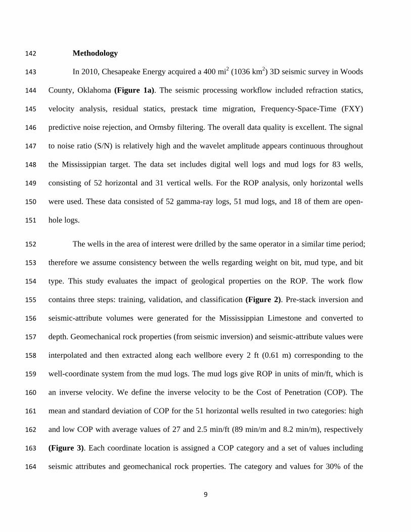
Methodology 142
In 2010, Chesapeake Energy acquired a 400 mi2 (1036 km2) 3D seismic survey in Woods 143
County, Oklahoma (Figure 1a). The seismic processing workflow included refraction statics, 144
velocity analysis, residual statics, prestack time migration, Frequency-Space-Time (FXY) 145
predictive noise rejection, and Ormsby filtering. The overall data quality is excellent. The signal 146
to noise ratio (S/N) is relatively high and the wavelet amplitude appears continuous throughout 147
the Mississippian target. The data set includes digital well logs and mud logs for 83 wells, 148
consisting of 52 horizontal and 31 vertical wells. For the ROP analysis, only horizontal wells 149
were used. These data consisted of 52 gamma-ray logs, 51 mud logs, and 18 of them are open-150
hole logs. 151
The wells in the area of interest were drilled by the same operator in a similar time period; 152
therefore we assume consistency between the wells regarding weight on bit, mud type, and bit 153
type. This study evaluates the impact of geological properties on the ROP. The work flow 154
contains three steps: training, validation, and classification (Figure 2). Pre-stack inversion and 155
seismic-attribute volumes were generated for the Mississippian Limestone and converted to 156
depth. Geomechanical rock properties (from seismic inversion) and seismic-attribute values were 157
interpolated and then extracted along each wellbore every 2 ft (0.61 m) corresponding to the 158
well-coordinate system from the mud logs. The mud logs give ROP in units of min/ft, which is 159
an inverse velocity. We define the inverse velocity to be the Cost of Penetration (COP). The 160
mean and standard deviation of COP for the 51 horizontal wells resulted in two categories: high 161
and low COP with average values of 27 and 2.5 min/ft (89 min/m and 8.2 min/m), respectively 162
(Figure 3). Each coordinate location is assigned a COP category and a set of values including 163
seismic attributes and geomechanical rock properties. The category and values for 30% of the 164

10
wells were used as inputs to train the model. The remaining 70% of the wells were used to 165
validate the model. When an optimal accuracy is reached, the model is used to classify the entire 166
data set where wells have yet to be drilled and no COP data are available. 167
Time-depth conversion 168
Formation tops for the Lansing, Mississippian and Woodford units were interpreted on 169
the time-migrated seismic data in the time domain and on well logs in the depth domain. A 170
conversion velocity model ( ( )0 , V x y ) was built using commercial software PETREL (© 171
Schlumberger), where velocity, V0 is defined at the top of the Lansing datum, ( )0 , Z x y . Depth, 172
Z, is calculated by adding the depth below the Lansing, ( ) ( )0 0, ,Z V x y t t x yΔ = × −⎡ ⎤⎣ ⎦ to the 173
datum. The well tops were used as a correction factor in the creation of the velocity model. Well 174
data were assigned more weights than the seismic data. We followed the recommended settings 175
to build the velocity model, such that a moving-average method was used as an interpolation 176
approach for creating the new depth surfaces and an inverse-distance-squared algorithm was 177
used to compute the inverse distance during the interpolation processes. Because the seismic 178
horizons honored the faults in the study area, the velocity model is computed taking faults into 179
consideration. 180
Geometric attributes 181
Geometric attributes for this dataset were generated using software AASPI developed at 182
the University of Oklahoma. The attributes generated included: most positive curvature, k1, most 183
negative curvature, k2, curvedness, 2 21 2k k+ , shape index, 2 1
2 1
2 ( )k ks ATANk kπ
+=−
, coherent 184
energy, and coherence. These attributes were chosen because of their ability to delineate the 185
11
structural complexity in the area of interest. The sampling interval of these attributes is the same 186
as the original seismic data volume, 110 ft by 110 ft (33.5 m by 33.5 m). In order to match the 187
mud log coordinate spacing, linear interpolation was used to generate values at 2 ft (0.61 m) 188
intervals. 189
Geomechanical rock properties 190
Geomechanical rock properties were derived from pre-stack inversion results using 191
commercial software Hampson Russell (© CGG GeoSoftware). Data preconditioning steps, prior 192
to a pre-stack seismic inversion included phase shift, bandpass filtering (10-15-110-120 Hz), 193
parabolic Radon transform, and trim statics. 194
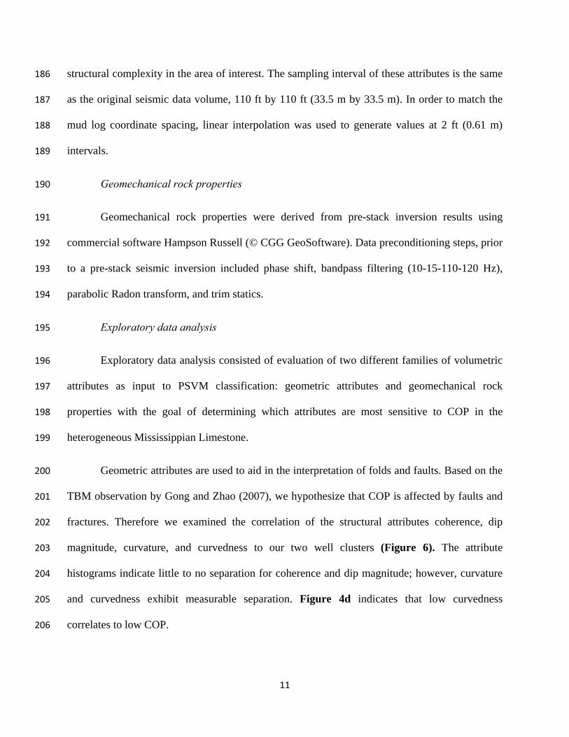
Exploratory data analysis 195
Exploratory data analysis consisted of evaluation of two different families of volumetric 196
attributes as input to PSVM classification: geometric attributes and geomechanical rock 197
properties with the goal of determining which attributes are most sensitive to COP in the 198
heterogeneous Mississippian Limestone. 199
Geometric attributes are used to aid in the interpretation of folds and faults. Based on the 200
TBM observation by Gong and Zhao (2007), we hypothesize that COP is affected by faults and 201
fractures. Therefore we examined the correlation of the structural attributes coherence, dip 202
magnitude, curvature, and curvedness to our two well clusters (Figure 6). The attribute 203
histograms indicate little to no separation for coherence and dip magnitude; however, curvature 204
and curvedness exhibit measurable separation. Figure 4d indicates that low curvedness 205
correlates to low COP. 206

12
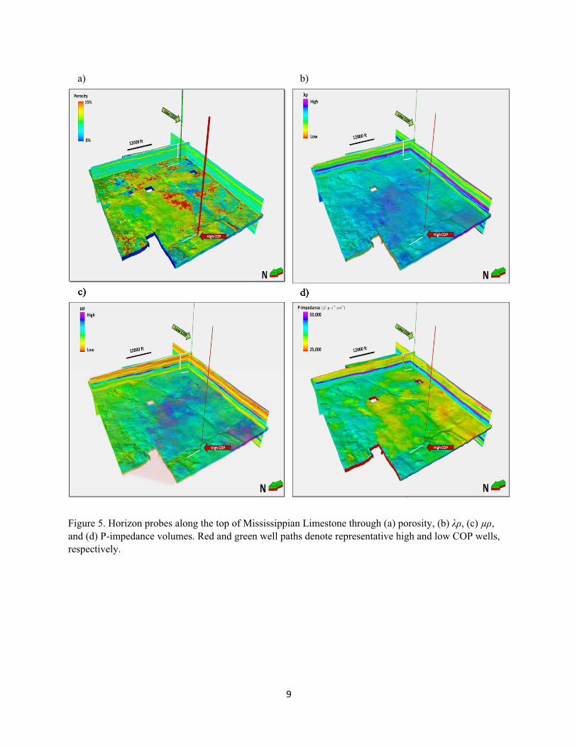
TBM analysis by Gong and Zhao (2007) also suggested that mechanical properties play a 207
significant role in the variation of COP. Using prestack seismic inversion we computed porosity, 208
lambda-rho, λρ , mu-rho, μρ , and P-impedance volumes to analyze the Mississippian Limestone 209
(Figure 5). The P-impedance measures the product of density and seismic P velocity. λρ and μρ 210
are used to estimate lithology and geomechanical behavior such as the brittleness index (Perez 211
and Marfurt, 2013). Figures 4b, 4c, and 4e show the high degree of separation for these rock 212
properties. Low COP is related to low porosity, high λρ, high μρ, and high P-impedance values. 213
Conversely, high porosity, low λρ, low μρ, and low P-impedance values are indicative of high 214
COP. These differences were used to train the PSVM model and classify COP data based on the 215
geomechanical rock properties within the Mississippian interval in the study area (Figure 10). 216
Results 217
Interactive Classification 218
The rectangular frame separating the dark gray circle from the light gray circle in Figure 219
7b is called a discriminator. Note that many of the measurements cannot be separated in Figure 220
7a. Because Gong and Zhao, (2009) found that increased brittleness improved TBM performance, 221
we examine brittleness as a means to predict COP. Altamar and Marfurt (2014) used 222
geomechanical properties to predict brittleness index for shale plays in the USA. We display a 223
crossplot in Figure 9 where each sample was color-coded bzy COP and plotted in a 2D space. 224
Then we manually defined high COP (red), low COP (green) and mixed COP (yellow) polygons 225
to define a 3-cluster template. A crossplot of λρ and μρ in Figure 9a illustrates the limitations of 226
manually picking clusters in two-attribute space, where 50% of the voxels fall into the mixed 227
COP (yellow) class. Figure 9b, a crossplot of ρ and Vp/Vs, further shows this problem with the 228
handpicked clusters where an even larger number of voxels falls into the mixed (yellow) class. 229

13
Figure 8 suggests improved class separation when using three attributes. However, drawing a 230
template is significantly more challenging than in Figure 6. 231
PSVM Classification 232
Visualization and interactive visualization with more than three attributes is intractable. 233
PSVM addresses this problem in two ways. First, it projects the data, in this case, two attributes 234
defining a 2D space that cannot be separated by a linear discriminator, into a higher 3-235
dimensional space (Figure 7) where separation by a planar discriminator is possible. Second, 236
because the discriminator generation is machine driven rather than interpreter driven, one can 237
introduce more than three input attributes. We used the five attributes, curvedness, λρ, μρ, 238
porosity, and P-impedance which found to exhibit good histogram separation in all exploratory 239
data analysis steps (Figure 3). The PSVM method allows us to create a classification model 240
based on a set of training input. As the dimensionality of the input increases, the model becomes 241
more accurate at classifying COP within the dataset. For instance, during the validation process, 242
we found the model to be sensitive to porosity. Before porosity was introduced to the model, the 243
accuracy was 88.9%. When porosity was added as a new degree of dimensionality, the accuracy 244
increased to 94%. This allowed for the creation of an optimal model with five degrees of 245
dimensionality for COP classification across the study area. 246
A comparison of the histograms (Figure 4) shows that the generated PSVM model is 247
more sensitive to geomechanical rock properties than geometric attributes. Indeed, strain 248
(measured by curvature) is only one component necessary to generate natural fractures. Stearns 249
(2015) found fractures measured in horizontal image logs were highly correlated to gamma ray 250
(lithology) response and only less connected to curvature, if at all. Nevertheless, this is not to say 251
structural attributes such as curvature have no effect on the model. We observed that higher COP 252

14
values are linked with higher curvedness, which indicated that it is harder to drill through the 253
formation with higher structural complexities. Studies have found that large curvature values are 254
related with natural fractures, which may or not be cemented (Bourgoyne et al., 1986; Hunt et al., 255
2011). Such heterogeneities may slow the drilling progress. Porosity is another a good indicator 256
of microstructures associated with fracture geometry. Low porosity observed in low COP wells 257
may seem counter-intuitive at first; however, woodworkers observe that there are few bit 258
problems when drilling through oak, but that the bit often gets stuck or even breaks when drilling 259
relatively “soft” pine (Neher, 1993). Again using the woodworker’s analogy, one uses different 260
saw blades for different woods. The bits used in this survey may have been chosen to deal 261
effectively with the very hard chert. 262
Conclusions 263
COP is a major factor affecting the time spent drilling a well and is directly related to the 264
overall cost of the drilling process. This is the first study that links COP to seismic data and 265
seismic-related attributes. Clustering five attributes using a PSVM classification method, we 266
were able to correlate COP with seismic attributes and geomechanical rock properties and obtain 267
a confidence of 94%. Low COP was observed in wells encountering low porosity, high λρ, high 268
μρ, low curvedness and high P-impedance. High COP was observed in wells encountering high 269
porosity, low λρ, low μρ, high curvedness and low P-impedance. By using this workflow, we can 270
use COP of previously drilled wells with 3D seismic data to predict COP over the study area. 271
While one may still wish to drill a specific target objective, we claim that this statistical analysis 272
technique will provide a more accurate cost estimate and help choose the appropriate drilling 273
equipment. 274
275

15
References 276
Altamar, R. P., and K. Marfurt, 2014, Mineralogy-based brittleness prediction from surface 277
seismic data: Application to the Barnett Shale: Interpretation, v. 2, no. 4, p. T255–T271, 278
doi:10.1190/INT-2013-0161.1. 279
Bass, N. W., 1942, Subsurface geology and oil and gas resources of Osage County, Oklahoma, in 280
U. S. Geological Survey Bulletin 900-K: p. 343–393. 281
Bourgoyne, A. T., K. K. Millheim, M. E. Chenevert, and F. S. Young Jr, 1986, Applied Drilling 282
Engineering Chapter 8 Solutions. Society of Petroleum Engineers. 283
Costello, D., M. Dubois, and R. Dayton, 2013, Core to characterization and modeling of the 284
Mississippian, North Alva area, Woods and Alfalfa Counties, Oklahoma, in 2013 Mid-285
Continent Section AAPG Core Workshop: from source to reservoir to seal: Wichita, KS, p. 286
165–175. 287
Dowdell, B. L., J. T. Kwiatkowski, and K. J. Marfurt, 2013, Seismic characterization of a 288
Mississippi Lime resource play in Osage County, Oklahoma, USA: Interpretation, v. 1, no. 289
2, p. SB97–SB108, doi:10.1190/INT-2013-0026.1. 290
Farrokh, E., J. Rostami, and C. Laughton, 2012, Study of various models for estimation of 291
penetration rate of hard rock TBMs: Tunnelling and Underground Space Technology, v. 30, 292
p. 110–123, doi:http://dx.doi.org/10.1016/j.tust.2012.02.012. 293
Gong, Q. M., and J. Zhao, 2009, Development of a rock mass characteristics model for TBM 294
penetration rate prediction: International Journal of Rock Mechanics and Mining Sciences, 295
v. 46, no. 1, p. 8–18, doi:http://dx.doi.org/10.1016/j.ijrmms.2008.03.003. 296

16
Gong, Q. M., J. Zhao, and Y. S. Jiang, 2007, In situ TBM penetration tests and rock mass 297
boreability analysis in hard rock tunnels: Tunnelling and Underground Space Technology, v. 298
22, no. 3, p. 303–316, doi:http://dx.doi.org/10.1016/j.tust.2006.07.003.Harris, N. B., J. L. 299
Miskimins, and C. A. Mnich, 2011, Mechanical anisotropy in the Woodford Shale, Permian 300
Basin: Origin, magnitude, and scale: The Leading Edge, v. 30, no. 3, p. 284–291, 301
doi:10.1190/1.3567259. 302
Hunt, L., S. Reynolds, S. Hadley, J. Downton, and S. Chopra, 2011, Causal fracture prediction: 303
Curvature, stress, and geomechanics: The Leading Edge, v. 30, no. 11, p. 1274–1286, 304
doi:10.1190/1.3663400. 305
King, C. H., and M. D. Pinckard, 2000, Method of and system for optimizing rate of penetration 306
in drilling operations, US6026912A: Google Patents. 307
Lindzey, K., M. J. Pranter, and K. Marfurt, 2015, Geologically Constrained Seismic 308
Characterization and 3-D Reservoir Modeling of Mississippian Reservoirs, North Central 309
Anadarko Shelf, Oklahoma, in AAPG Annual Convention and Exhibition, Tulsa, OK, USA. 310
Mazzullo, S. J., B. W. Wilhite, and I. W. Woolsey, 2009, Petroleum reservoirs within a spiculite-311
dominated depositional sequence: Cowley Formation (Mississippian: Lower Carboniferous), 312
south-central Kansas: AAPG bulletin, v. 93, no. 12, p. 1649–1689. 313
Montgomery, S. L., J. C. Mullarkey, M. W. Longman, W. M. Colleary, and J. P. Rogers, 1998 314
Mississippian “Chat” Reservoirs, South Kansas: Low-Resistivity Pay in a Complex Chert 315
Reservoir: AAPG Bulletin, v. 82, p. 187-205. 316
317

17
Neher, H. V., 1993, Effects of pressures inside Monterey pine trees: Trees, v. 8, no. 1, p. 9–17, 318
doi:10.1007/BF00240976. 319
Parham, K. D., and R. A. Northcutt., 1993, Mississippian chert and carbonate basal 320
Pennsylvanian sandstone; Central Kansas Uplift and northern Oklahoma, in Atlas of major 321
midcontinent gas reservoirs: Texas Bureau of Economic Geology, Austin, TX, Gas 322
Research Institute. 323
Perez, R., and K. Marfurt, 2013, Brittleness estimation from seismic measurements in 324
unconventional reservoirs: Application to the Barnett Shale, in 2013 SEG Annual Meeting, 325
Houston, TX, USA. 326
Rogers, S. M., 2001, Deposition and diagenesis of Mississippian chat reservoirs, North-Central 327
Oklahoma: AAPG Bulletin, v. 85, no. 1, p. 115–129, doi:10.1306/8626C771-173B-11D7-328
8645000102C1865D. 329
Roy, A., B. L. Dowdell, and K. J. Marfurt, 2013, Characterizing a Mississippian tripolitic chert 330
reservoir using 3D unsupervised and supervised multiattribute seismic facies analysis: An 331
example from Osage County, Oklahoma: Interpretation, v. 1, no. 2, p. SB109–SB124, 332
doi:10.1190/INT-2013-0023.1. 333
Da Silva, M., and K. Marfurt, 2012, Framework for EUR correlation to Seismic Attributes in the 334
Barnett Shale, TX, in 2012 SEG Annual Meeting, Las Vegas, NV, USA. 335
Stearns, V. T., 2015, Fracture characterization of the Mississippi lime utilizing whole core, 336
horizontal borehole images, and 3D seismic data from a mature field in Noble County 337
Oklahoma: MS thesis University of Oklahoma. 338

18
Verma, S., O. Mutlu, and K. J. Marfurt, 2013, Seismic modeling evaluation of fault illumination 339
in the Woodford Shale, in 2013 SEG Annual Meeting, Houston, Texas USA. 340
Verma, S., T. Zhao, K. J. Marfurt, and D. Devegowda, 2016, Estimation of total organic carbon 341
and brittleness volume: Interpretation, v. 4, no. 3, p. T373–T385, doi:10.1190/INT-2015-342
0166.1. 343
Watney, W. L., W. J. Guy, and A. P. Byrnes, 2001, Characterization of the Mississippian chat in 344
south-central Kansas: AAPG bulletin, v. 85, no. 1, p. 85–113. 345
White, H., B. Dowdell, and K. J. Marfurt, 2012, Calibration of surface seismic attributes to 346
natural fractures using horizontal image logs, Mississippian Lime, Osage County, 347
Oklahoma, in 2012 SEG Annual Meeting, Las Vegas, NV, USA. 348
Zhang, B., T. Zhao, X. Jin, and K. Marfurt, 2015, Brittleness evaluation of resource plays by 349
integrating petrophysical and seismic data analysis: Interpretation, v. 3, no. 2, p. T81–T92, 350
doi:10.1190/INT-2014-0144.1. 351
Zhao, T., V. Jayaram, K. J. Marfurt, and H. Zhou, 2014, Lithofacies classification in Barnett 352
Shale using Proximal Support Vector Machines, in 2014 SEG Annual Meeting, Denver, CO, 353
USA. 354
355
Zhao, T., V. Jayaram, A. Roy, and K. J. Marfurt, 2015, A comparison of classification 356
techniques for seismic facies recognition: Interpretation, v. 3, no. 4, p. SAE29–SAE58, 357
doi:10.1190/INT-2015-0044.1. 358
359

1
Figure captions
Figure 1. (a) Major geologic provinces of Oklahoma with the area of interest outlined in red. (Modified
from Johnson and Luza (2008); Northcutt and Campbell (1996)). (b) a type log showing the Mississippian
Limestone section in the area of interest (Modified from Lindzey et al., 2015).
Figure 2. (a) Workflow for attribute generation and depth conversion, (b) data analysis of the extracted
parameters, (c) the training process, and (d) the validation process.
Figure 3. The mean and standard deviation of COP for 51 horizontal wells that fall within the 3D seismic
survey. We separate these wells into two classes: seven high COP (the grey cluster) and forty-four low COP
wells (the white cluster). The dashed line is called the discriminator between the two clusters.
Figure 4. Exploratory data analysis using the work flow shown in Figure 2b. Showing five attributes
exhibiting good histogram separation between high COP (in dark gray) and low COP (in light gray) along
all well trajectories: (a) curvedness, (b) , (c) , (d) P-impedance, and (e) porosity. (f) Results of the
validation test using seven low and seven high COP wells which are highlighted by gray circle in Figure 3.
With increases in the number of inputs (from one to five), the accuracy increases accordingly.
Figure 5. Horizon probes along the top of Mississippian Limestone through (a) porosity, (b) , (c) , and
(d) P-impedance volumes. Red and green well paths denote representative high and low COP wells,
respectively.
Figure 6. Co-rendered the most positive (k1) and the most negative (k2) curvature along the top of the
picked Mississippian horizon with two representative high and low COP wells paths. The opacity curve is
applied to k1 and k2.
Figure 7. (a) when two different clusters are impossible to separate by a line in a 2-D space. (b) increasing
the dimensionality to 3 through a nonlinear attribute transformation allows separation of the two classes by
a plan.

2
Figure 8
2-D space. (b) Discrimination becomes easier by adding a third porosity axis.
Figure 9. -
triplets. Each sample is color- -
mixed cluster polygons are hand-drawn polygons around each cluster. This template is then used to color-
code voxels between the top of the Mississippian Limestone and the top of Woodford. Red and green well
paths denote representative high and low COP wells. In (b) -Vp/Vs
Vp/Vs and COP are sampled along the wellbore, crossplotted, and a new template constructed and used to
color code the Mississippian interval. Note that neither template accurately predicts the COP of these two
wells.
Figure 10. Horizon probe of COP on the Mississippian Limestone computed using the five attributes shows
in Figure 4-6 and a PSVM classifier. Note that the two representative wells now fall along voxels
corresponding to their observed COP value.

3
a)

4
Figure 1. (a) Major geologic provinces of Oklahoma with the area of interest outlined in red.
(Modified from Johnson and Luza (2008); Northcutt and Campbell (1996)). (b) a type log showing the
Mississippian Limestone section in the area of interest (Modified from Lindzey et al., 2015).
b)

5
a)
-
b)

6
c)
d)
Figure 2. (a) Workflow for attribute generation and depth conversion, (b) data analysis of the extracted
parameters, (c) the training process, and (d) the validation process.

7
Figure 3. The mean and standard deviation of COP for 51 horizontal wells that fall within the 3D
seismic survey. We separate these wells into two classes: seven high COP (the grey cluster) and forty-
four low COP wells (the white cluster). The dashed line is called the discriminator between the two
clusters.
Discriminator

8
Figure 4. Exploratory data analysis using the work flow shown in Figure 2b. Showing five attributes exhibiting good histogram separation between high COP (in dark gray) and low COP (in light gray) along all well trajectories: (a) curvedness, (b) , (c) , (d) P-impedance, and (e) porosity. (f) Results of the validation test using seven low and seven high COP wells which are highlighted by gray circle in Figure 3. With increases in the number of inputs (from one to five), the accuracy increases accordingly.
9
Figure 5. Horizon probes along the top of Mississippian Limestone through (a) porosity, (b) , (c) , and (d) P-impedance volumes. Red and green well paths denote representative high and low COP wells, respectively.
a) b)
d) c)

10
Figure 6. Co-rendered the most positive (k1) and the most negative (k2) curvature along the top of the picked Mississippian horizon with two representative high and low COP wells paths. The opacity curve is applied to k1 and k2.

11
Figure 7. (a) when two different clusters are impossible to separate by a line in a 2-D space. (b) increasing the dimensionality to 3 through a nonlinear attribute transformation allows separation of the two classes by a plan.

12
Figure 8. (a) Similarly, high and low COP is difficult to discriminate when using and curvedness in a 2-D space. (b) Discrimination becomes easier by adding a third porosity axis.

13
Figure 9. (a) -triplets. Each sample is color-coded along the well by its COP - reen and mixed cluster polygons are hand-drawn polygons around each cluster. This template is then used to color-code voxels between the top of the Mississippian Limestone and the top of Woodford. Red and green well paths denote representative high and low COP wells. In (b) -Vp/Vs space.
p/Vs and COP are sampled along the wellbore, crossplotted, and a new template constructed and used to color code the Mississippian interval. Note that neither template accurately predicts the COP of these two wells.
(a)
(b)

14
Figure 10. Horizon probe of COP on the Mississippian Limestone computed using the five attributes shows in Figure 4-6 and a PSVM classifier. Note that the two representative wells now fall along voxels corresponding to their observed COP value.