‘particulate matter removal in automotive after...
TRANSCRIPT

‘Particulate matter removal in automotive after-treatment systems’ Master Thesis in the Master’s programme in Innovative and Sustainable Chemical
Engineering (MPISC)
ANANDA SUBRAMANI KANNAN
HOUMAN OJAGH
Department of Applied Mechanics
Division of Combustion and Division of Fluid dynamics
CHALMERS UNIVERSITY OF TECHNOLOGY
Göteborg, Sweden 2013
Master‘s thesis 2013:33

MASTER THESIS IN INNOVATIVE AND SUSTAINABLE CHEMICAL
ENGINEERING (MPISC)
‘Particulate matter removal in automotive after-treatment
systems‘
ANANDA SUBRAMANI KANNAN
HOUMAN OJAGH
Department of Applied Mechanics
Division of Combustion and Division of Fluid dynamics
CHALMERS UNIVERSITY OF TECHNOLOGY
Göteborg, Sweden 2013

Particulate matter removal in automotive after-treatment systems
ANANDA SUBRAMANI KANNAN
HOUMAN OJAGH
© ANANDA SUBRAMANI KANNAN AND HOUMAN OJAGH, 2013
Master Thesis 2013:33
ISSN 1652-8557
Department of Applied Mechanics
Division of Combustion and Division of Fluid dynamics
Chalmers University of Technology
SE-412 96 Göteborg
Sweden
Telephone: + 46 (0)31-772 1000
Cover:
Modified exhaust after treatment system.
Chalmers reproservice
Göteborg, Sweden 2013

I
Particulate matter removal in automotive after-treatment systems
Master Thesis in the Master’s programme in Innovative and Sustainable Chemical
Engineering (MPISC)
ANANDA SUBRAMANI KANNAN
HOUMAN OJAGH Department of Applied Mechanics
Division of Combustion and Division of Fluid dynamics
Chalmers University of Technology
ABSTRACT
There is growing concern in the world with regard to pollution and climate change.
The relation between air pollution and climate change in particular is strong and
complex. There is thus a shift towards greener technologies and a large amount of
resources have been allocated for the research and development of such technologies.
As emission regulations are becoming stricter, there is a concerted effort from all
fronts in the EU to design and develop an optimal exhaust after-treatment system
which would concur with current emission regulations imposed by Euro V and Euro
VI (0.005 g/km of particulate matter (PM) and particulate number (PN) 6.0×10¹¹
) for
both gasoline and diesel powered drives). Open channel substrates (described in this
work) are used for the removal of particulate matter from exhaust. Such substrates are
made of channels (arranged in a honeycomb structure) which permit the flow of
exhaust through them. The PM is ultimately trapped on the wall of these channels.
Over the past decade there has been a substantial increase in the computational power
available to researchers. This increase of available computational resources has
shifted the prime focus of research from time-consuming and expensive construction
of pilot-scale prototypes towards simulation-driven development of new after
treatment solutions. The current work aims to describe such a feedback between
experiments and simulations in order to describe the capture of an inert particle
(sodium chloride - NaCl) in an open substrate (monolith channel). The experiments
and simulations are done in conjunction and such a systematic approach improves the
quality of the experimental evaluation. This congruence is evident throughout this
work, with the simulations generally, corresponding to the experimental results
(simulations results are within the error limit of the experimental results). Both
temperature and residence time have a significant impact on the capture efficiency
due to Brownian deposition along an open channel. In addition the general trends with
variation in residence time (flow conditions) and temperature are noticeably similar in
both experiments and simulations. This indicates that the theory behind the
description of capture efficiency in open channels (Brownian deposition in open
substrates) is able to explain the capture phenomena of inert particulates accurately.
Key words: Computational, Brownian deposition, Capture efficiency, Inert
particulates, Particulate matter, Particulate number, Open substrates

CHALMERS, Applied Mechanics, Master‘s Thesis 2013:33 II
Contents
1 INTRODUCTION 1
1.1 Background 1
1.2 Problem description 2
1.3 Objectives of this work 2
1.4 Theory 3
1.4.1 Particulate matter (PM) 3
1.4.2 Exhaust after-treatment systems 4 1.4.3 Numerical aspects of modelling PM capture in open substrates 6
2 EXPERIMENTAL SET-UP 15
2.1 Related apparatus 15 2.1.1 TOPAS-ATM230 15 2.1.2 DMS500 16
2.1.3 The EATS (emission after treatment system) 16
2.2 Initial trials 18
2.2.1 Preparation of salt solutions 18
2.2.2 Preliminary trials and experimental design (1st and 2
nd sets) 18
2.2.3 Particle size measurements 20 2.2.4 The capture efficiency trials (3
rd set) 21
2.3 Strategy adopted in this study 24
3 SIMULATIONS 25
3.1 EATS simulations 25 3.1.1 EATS geometry 25 3.1.2 EATS meshing 27 3.1.3 Set-up and Boundary conditions 27
3.2 Single channel simulations 29 3.2.1 Channel geometry 29
3.2.2 Single channel meshing 29 3.2.3 Channel Set-up and Boundary conditions (Theoretical capture
efficiency) 30
4 RESULTS AND DISCUSSION 33
4.1 Results of the initial trials (1st & 2
nd sets) 33
4.1.1 Effect of concentration 33 4.1.2 Effect of the atomizer pressure (up-stream pressure) on PSD 34
4.1.3 Particle size measurement evaluation 34
4.2 Results from the initial simulations 36 4.2.1 Results from the EATS simulations 36 4.2.2 Studies on the temperature profile within the EATS (without the flow
straighteners) 37

CHALMERS, Applied Mechanics, Master‘s Thesis 2013:33 III
4.3 Experimental CE trials 39 4.3.1 Capture efficiency for the non-adiabatic conditions (Case A) 39 4.3.2 Capture efficiency for the adiabatic conditions (Case B) 40 4.3.3 Comparison between non-adiabatic and adiabatic conditions (Case C)
42
4.4 Results from single channel capture efficiency simulations (theoretical CE)
43 4.4.1 Adiabatic channel simulations 43 4.4.2 Non-Adiabatic channel simulations 45
4.4.3 Results from the Johnson and Kittleson correlations 46
4.5 Comparison between experiments and simulations 48
4.5.1 Comparison under adiabatic conditions 48 4.5.2 Comparison under non-adiabatic conditions 49
5 CONCLUSIONS AND RECOMMENDATIONS 51
5.1 Conclusions 51
5.2 Recommendations and future work 52
6 REFERENCES 55
7 APPENDICES 59
Appendix I: Creeping flow calculations 59
Appendix II: Published values of Knudsen-Weber slip correction parameters for the
correction of stokes law) 59
Appendix III: TOPAS ATM-230 operating pressure and recirculation ratio 60
Appendix IV: Preliminary trials 61 a) First sets of experiments 61
b) Second set of experiments 64
Appendix V: EATS flow calculations (Reynolds number calculations for EATS
inlet and monolith channel) 65 a) Re at the EATS inlet 65 b) Re in the channel 65
Appendix VI: Typical values of C2 (viscous resistance factor) along with the
corresponding monolith pressure drops 66
Appendix: VII UDF‘s 66 Diffusivity 66 Wall temperature profile 67
Appendix VIII: Mesh quality study 68 a) EATS 68 b) Channel 69
Appendix IX: Temperature profile comparison between experiments and
simulations 71
Appendix X: Sample time stability assessments 72

CHALMERS, Applied Mechanics, Master‘s Thesis 2013:33 IV
Appendix XI: CE Experiments 73 Appendix XII: Non-adiabatic set up (Case II) 79 Appendix XIII: Adiabatic set up (Case I) 81 Appendix XIV 83
Appendix XV: Temperature profile comparison from simulations 84
Appendix XVI: Comparison between experiments and simulations 85 a) Adiabatic conditions 85 b) Non adiabatic conditions 87
Appendix XVII: Sensitivity Analysis 88 Effect of monolith choice (channel hydraulic diameter) on CE 88 Effect of temperature on CE 89 Effect of engine exhaust flow on CE 89
Appendix XVIII: Accuracy of CFD results 92
Appendix XIX: Comparison between theory and simulations (Validation of CFD
results) 93

CHALMERS, Applied Mechanics, Master‘s Thesis 2013:33 V
Preface
This master thesis has been conducted for the fulfilment of the Master of Science
degree in Innovative and sustainable chemical engineering at Chalmers University of
technology, Göteborg, Sweden. In this thesis, experimental and numerical evaluations
(CFD simulations) have been performed in order to describe the capture of an inert
particle (sodium chloride - NaCl) in an open substrate (monolith channel). These have
been done in conjunction and such a systematic approach has thus improved the
quality of the experimental evaluation. The thesis has been carried out from January
2013 to June 2013.
The thesis has been executed under the supervision of Dr. Jonas Sjöblom (Assistant
professor at the Division of Combustion) and Dr. Henrik Ström (Post-doctoral
researcher at the Division of fluid dynamics) at Chalmers University of technology.
We would like to thank both Jonas and Henrik , who have been our mentors, for their
constant guidance and support. This thesis would not have materialized without their
vision. We would also like to thank our examiners Sven Andersson (Associate
professor at the Division of Combustion) and Srdjan Sasic (Associate professor at the
Division of fluid dynamics) for their for their guidance and technical insights during
the course of our research. All experimental trials have been carried out in the
research laboratories of the Division of combustion at Chalmers University of
Technology, Göteborg. We would like to extend our heartfelt gratitude towards all the
support staff at the labs - Alf Magnusson, Eugenio De Benito Sienes and Daniel
Härensten for providing pragmatic and rapid solutions to some of the problems
encountered during the experimental trials.
Finally, we would like to thank our family and friends who have stood by us through
the entire period and have made this experience a memorable one.
Göteborg June 2013
Ananda Subramani Kannan
Houman Ojagh

CHALMERS, Applied Mechanics, Master‘s Thesis 2013:33 VI
ABBREVIATIONS
CE Capture efficiency
DL Diffusion losses
DOC Diesel oxidation catalyst
DPF Diesel particulate filter
EATS Exhaust after treatment system
HC Hydrocarbon
EC Elemental carbon
NOx Nitrous oxide and Nitrogen dioxide
PE Penetration efficiency
PM Particulate matter
PN Particulate number
TWC Three way catalyst
Nomenclature list
Α Parameter vector for secondary dilutor losses [m2s
-1]
A‘ Coefficient [-]
αc Condensation coefficient [-]
α, β and γ Experimentally determined coefficients [-]
AS Surface area (channel) [m2]
Aw Area (pocket wall) [m2]
C Cunningham correction factor [-]
CD Drag coefficient [-]
CE Capture efficiency [%]
Dab Diffusion coefficient [m2s
-1]
Dp Particle diffusivity [m2s
-1]
dh Channel hydraulic diameter [m]
dp Particle diameter [m]

CHALMERS, Applied Mechanics, Master‘s Thesis 2013:33 VII
dt Tube diameter [m]
Ε Uncertainty measure for CE [%]
gi Acceleration due to gravity [ms-2
]
hm Average mass transfer coefficient [ms-1
]
Ji Diffusion flux of species ‘i’ [cm-2
s-1
]
kB Boltzmann constant [J]
Kn Knudsen number [-]
L Characteristic pipe Length [m]
Λ Mean free path [nm]
M Molecular mass [kg/mole]
min,mout Mass in and mass out over a differential volume [kg]
µ Dynamic viscosity [Pas]
Nin, Nout Number of particles [Ncm-3
]
NA Avogadro‘s number [mole-1
]
p∞, pd partial pressure in bulk, at particle surface [Pa]
PE Penetration efficiency [%]
PSD Particle size distribution [dN/dlog(dp)]
Q Volumetric flow rate [m3s
-1], [dm
3min
-1]
Re, Rep Reynolds number and particle Reynolds number [-]
Ri The net rate of production of species ‘i’ by
chemical reaction
[mols-1
]
ρg, ρp Density for gas, particle [kgm-3
]
Sh Sherwood number [-]
T Temperature [K], [°C]
UjUi,,U Average linear (pipe) velocity [ms-1
]
V Volume [m3]
Vd Deposition velocity [ms-1
]
X, Yi Mass fraction [-]
x, y Space coordinates [m]


CHALMERS, Applied Mechanics, Master‘s Thesis 2013:33 1
1 Introduction
This section gives the background to this work and describes the primary objectives that are to be
achieved. The aim is defined together with a brief review of relevant works which put the current
study into perspective.
1.1 Background
There is growing concern in the world with regard to pollution and climate change. The relation
between air pollution and climate change in particular is strong but complex (EEA, 2012). There
is thus a shift towards greener technologies and a large amount of resources have been allocated
to research and develop such technologies.
Vehicles that run on carbon based fuels are the primary contributors to many different air
pollutants such as carbon monoxide (CO), various hydrocarbons (HC), nitrogen oxides (NOx),
particulate matter (PM) and finally carbon dioxide (CO2). The presence of CO and HC is due to
incomplete combustion, whereas NOx is mainly formed from nitrogen in the air due to the high
temperatures inside the engine and at the end carbon dioxide (CO2) is formed as the final product
of fossil fuel combustion. The particulate matter (PM) emissions from engines are composed
predominantly of elemental carbon (EC or soot), organic carbon (HC) and sulphates. The
elemental fraction stems from fuel droplet pyrolysis, while the organic fraction originates from
unburned fuel, lubricating oil, and combustion by-products (Shah, Cocker, Miller, & Norbeck,
2004). These PM emissions from diesel engines are a significant source of small (< 2.5 µm)
particles in urban areas, and epidemiology has demonstrated that susceptible individuals are
being harmed by ambient particulate matter (Lighty, 2004). Reducing these emissions may warm
or cool the atmosphere because several of these pollutants demonstrate a positive or a negative
climate-forcing impact, either directly or indirectly (EEA, 2012). The direct climatic impacts
include effects of sulphate aerosols which reflect solar radiation leading to net cooling and the
effects of EC aerosols which absorb solar radiation leading to warming. Indirect impacts include
aerosols altering cloud properties and NOx promoting tropospheric O3 formation that warms the
atmosphere and acid rain (Balkanski et al., 2010).
In addition, higher emission of carbon dioxide (CO2) as a greenhouse gas leads to higher
concentrations in the atmosphere that affects the biological carbon cycle. In other words, CO2
contributes to global warming (Cox, Betts, Jones, Spall, & Totterdell, 2000).
In order to meet the challenges from upcoming legislation and to contribute to a sustainable
future, emissions and the contents of particulate matter in engine exhaust must be reduced in
terms of both mass and number. In conventional stoichiometric gasoline engines, the three-way
catalyst (TWC) can be used to oxidize CO and HC and reduce NOx simultaneously. However,
CO2 cannot be converted over this catalyst. If emissions of CO2 are to be reduced, there must
instead be a change of fuel, an increase in fuel efficiency and/or an overall change of engine
technology (e.g. from combustion engine to fuel cell or electrical battery) (Ström, 2011).
Over the past decade there has been a substantial increase in the computational power available
to researchers. This increase of available computational resources has shifted the prime focus of
research from time-consuming and expensive construction of pilot-scale prototypes towards
simulation-driven development of new after treatment solutions. Not only are there huge savings

CHALMERS, Applied Mechanics, Master‘s Thesis 2013:33 2
to be made on cutting the design and development time (Oberkampf & Trucano, 2002), but also
computational simulations can often provide more information than what is available from
traditional experimental techniques. Hence the use of experimental investigations in conjunction
with mathematical modelling (using say computational fluid dynamics (CFD)) would provide a
comprehensive insight into any system being studied.
The following master thesis aims to describe the capture of an inert particle Sodium Chloride
(NaCl), in a monolith channel. Monoliths are configurations that contain several types of
interconnected or divided channels (straight, wavy or crimped) in one single chunk of material
(e.g. honeycombs, foams or interconnected fibres). The channels of the most common
honeycomb monoliths normally have circular, square or triangular cross sections. The capture
efficiency of the channel is estimated using PM measurements of the flow entering and leaving
the channel. In addition, numerical modelling (using CFD) of the same capture phenomenon is
also detailed in order to supplement the experimental findings. This co-dependency between the
two afore-mentioned strategies forms the crux of the work being presented in this dissertation.
1.2 Problem description
An extensive investigation of capture phenomena (including experimental trials and numerical
simulations) of diesel particulate matter in open substrates has recently been performed at the
research labs in the Division of combustion, Department of Applied mechanics, Chalmers
University of Technology, Göteborg (Sjöblom & Ström, 2013). The aim of this work was to
compare theoretical models for PM capture (achieved using CFD simulations) with experimental
results in order to correlate theory with experiments. However, due to inherent complexities
encountered during their study, there were strong dissimilarities between experiments and
simulations. These dissimilarities were later attributed to the model used for the simulations,
which assumed that diesel particulate matter is inert in nature (which is not necessarily true). A
simple conceptual model was therefore constructed to explain the experimental findings and fit it
closely with the simulations. This model accounted for loss of material by total evaporation (of
particles that are entirely made out of HCs) as well as by shrinkage (by evaporation from
particles with condensed HCs on their surface). It must be noted that, this model is valid only if it
can be confirmed that the CFD simulations and experimental trials are indeed comparable for an
inert substance. Thus a new study project to investigate the capture phenomena of inert solid
particles (instead of diesel particulate matter) in open substrates was proposed.
1.3 Objectives of this work
Capture efficiency experiments and simulations were planned in order to achieve congruence
between theory and experiments. The size dependent capture efficiency is evaluated and
compared with numerical simulations, showing how various transport processes (diffusion,
evaporation etc.) influence the capture results. In addition, the other goals of this work can be
summarized as follows –
Examine the possibility to generate and measure inert particles using an aerosol
generator.
Design and conduct experiments that will enable a close comparison with
computational fluid dynamics (CFD) simulations as well as produce a robust
methodology for PM measurements (including the design of thermo couple probe
positions, sample flow conditions and PM instrument settings (dilution factors)).

CHALMERS, Applied Mechanics, Master‘s Thesis 2013:33 3
Identify appropriate operating conditions while performing studies on open substrates
Simulate flow and PM motion in a single monolith channel.
1.4 Theory
As explained earlier, the primary objective of this work is to describe the capture phenomena in
open substrates. This would thus entail a brief description of particulate matter capture in
conventional exhaust after-treatment systems and a general outlook on PM measurements. A
brief description of numerical modelling approaches for PM capture in monoliths is also
provided in order to elucidate the fundamental concepts behind the simulations which would be
presented later in this work.
1.4.1 Particulate matter (PM)
Particulate matters from diesel engines (PM) are generally defined as solid or liquid particles
made of elemental carbon (EC), adsorbed hydrocarbons (HC) and inorganic compounds such as
sulphates, metallic compounds and water formed during exhaust dilution and cooling (Hinds,
1999). Yet, the most common definition of PM states everything that is collected on a filter paper
in exhaust that has been diluted and cooled to 52°C (SAE, 1993). Figure 1.1 illustrates idealized
number and mass weighted size distributions for diesel particulate matter. PM follows a
lognormal, tri-modal size distribution with the concentration in any size range being proportional
to the area under the corresponding curve in that range.
Figure 1.1- Illustration of the size distribution of diesel particulate matter (figure adapted from - (Kittelson, 1998))
Nuclei-mode, which are the smallest and primary particles formed during the combustion in the
engine cylinder, range in diameter from about 5 to 50 nm. The nuclei-mode (refer Figure 1.1
above) also includes droplets that nucleate upon cooling of the exhaust. These usually contain 1-
20 % of the particle mass and more than 90 % of the total particle number. The accumulation
mode ranges in size from roughly about 30 to 500 nm. Most of the mass is composed primarily

CHALMERS, Applied Mechanics, Master‘s Thesis 2013:33 4
of carbonaceous agglomerates and adsorbed materials. Finally, the coarse mode consists of
particles larger than about 1 (μm) and typically contains 5-20 % of the diesel particulate matter
mass (Kittelson, 1998).
1.4.2 Exhaust after-treatment systems
As emission regulations are becoming stricter, there is a concerted effort from all fronts in the
EU to design and develop an optimal exhaust after-treatment system which would concur with
current emission regulations imposed by Euro V and Euro VI (0.005 g/km of PM and PN
6.0×10¹¹
) for both gasoline and diesel powered drives)(Euro-5/6-Standards, 2009). The design of
such a system is complex and would require the combined effect of several individual emission
abatement technologies. The most commonly employed emission control technologies in a diesel
driven system are – diesel oxidation catalyst (DOC), diesel particulate filter (DPF) and diesel
NOx reduction filter (DeNOx). A schematic figure of an after-treatment system employing these
three filters is presented in the figure below.
Figure 1.2- An integrated soot-NOx emission control system (Figure adapted from Konstandopoulos et.al 2004)
The DOC (diesel oxidation catalyst) is a monolithic reactor which is designed to effectively
oxidize gaseous pollutants. In this way, the usual products of incomplete combustion, carbon
monoxide (CO) and various hydrocarbons (HC) , are finally converted into carbon dioxide (CO2)
and water (H2O). Since the diffusion of particulate matter to the catalytically active walls of the
standard monolithic reactor is very slow and ineffective, the monolithic reactor has not been
successful at reducing the particulate matter content and comply with legislation in its original
design (Ström, 2011). The wall-flow diesel particulate filter (DPF) is instead the most commonly
used reactor for removal of particulate matter in diesel applications (Konstandopoulos &
Kostoglou, 2004).
Since the current work focuses particularly on PM capture, the DPF would be the most apt
system to describe in order to put this work in perspective. There are a variety of DPFs available.
For example, the DPF could be made of composite fibrous materials which utilize fine fibres as a
means of particle filtration. The DPF may also be an extruded wall-flow monolithic filter, which
is commonly made of cordierite or silicon carbide material. A wall-flow monolith is the most
common type of filtration element employed. In such a DPF, every second channel in the
ceramic monolithic reactor is plugged in either end, creating a chessboard-like appearance of the
monolith front and back (Adler, 2005). The exhaust gas is therefore only allowed to enter the
channels which are open towards the inlet side, the so-called inlet channels. The gas is then
forced to flow through the porous wall into the four adjacent outlet channels. The DPF
accumulates particles on the inside and on the porous walls of the inlet channels (Liu, Berg,

CHALMERS, Applied Mechanics, Master‘s Thesis 2013:33 5
Swor, & Schauer, 2008). The main technical challenge for DPF systems in automotive
applications is their regeneration from the soot they retain from the exhaust gases (Vaaraslahti,
Virtanen, Ristimäki, & Keskinen, 2004).
Figure 1.3 – Standard DPF (left) (Figure courtesy of Northeast remaps Durham DPF removal). DPF design (right)- The
channels are plugged in either end (grey), forcing the gas to flow through the walls (arrows) and the soot (black) is
deposited along the inlet channels.(Figure courtesy of Castrol Lubricants, Division of BP EUROPA SE - BP
NETHERLANDS)
The work described here pertains to exhaust flow through open filters. This filter is very similar
to a DPF in its design and operation, the only difference being that no channels are plugged. This
would mean that the exhaust gas would flow through each and every channel unhindered. Such
open filters (with low pressure drop) have potential for efficient reduction of particulate matter
from diesel driven systems. The core component of both the DPF and open filter is the monolith
channel alone, as it is along the wall of these channels that PM trapping is achieved.
Monolithic reactors are either made of porous catalytic material or channels that are filled with
layers called washcoat which contain catalytic material in the empty space (porous zone). In both
arrangements, the channels provide the space for the flow of gas and/or liquid. Presently,
ceramic and metallic monoliths are the two major types of monolith supports that are used in
both industry and research. In the case of the square-channel monolith, the monolith geometry is
fully defined by three parameters: channel size (dh), wall thickness (Wt) or cell density (n) and
the channel length (L). If the monolith is extruded from a catalytic material, the amount of
catalyst in the unit volume of the reactor is fully determined by the monolith (Tomašić & Jović,
2006). The channels of the substrate have square cross-sections, which are rounded by the
washcoat as it is deposited onto the channel walls. Among these parameters, channel size and
shape affect the pressure drop across the channel and the hydrodynamics of the flow. A typical
ceramic substrate design is illustrated in the figure below –
Figure 1.2- Illustration of the monolith channels (Figure courtesy of (Creaser, 2013))

CHALMERS, Applied Mechanics, Master‘s Thesis 2013:33 6
1.4.3 Numerical aspects of modelling PM capture in open substrates
The capture of PM in open substrates is very complex to model. These complexities stem from
the wide variety of time and length scales that need to be independently resolved by a
computational grid in order to adequately describe the phenomenon. In addition, due to the
simultaneous interaction between the two phases (solid particles and exhaust gases) within the
system, the solution to such a numerical problem is complicated further. There are several
strategies that have been described in literature in order to model and simulate these complex
multiphase phenomena. Such simulations of multiphase and multicomponent flows pose greater
challenges than that of single-phase and single-component flows primarily due to the interfaces
between phases and the large or discontinuous property variations across these interfaces
between the phases and/or components (Hanratty et al., 2003). The strategies adopted to model
such a system (a dispersed gas-solid system) are described below.
The continuum framework and Navier-Stokes equations
The concept of the continuum is important in the development of equations for multiphase flows.
A fluid is regarded as consisting of continuous matter for which properties such as density and
velocity vary continuously from point to point. This idea is important in the development of the
differential forms of the conservation equations (Crowe, Schwarzkopf, Sommerfeld, & Tsuji,
2011). A fluid is typically composed of a vast number of molecules. There are for example more
than 1025
molecules in one cubic meter of air at room temperature and atmospheric pressure. It is
therefore not realistic to predict the individual motion of all the molecules contained within a
system. However, if the smallest volume of interest in an analysis still contains a sufficient
number of molecules, it is possible to obtain meaningful statistical averages. The molecules are
then treated as a continuous distribution of matter, i.e. as a continuum.
The Navier-Stokes equations (basic governing equations for a viscous, heat conducting fluid) are
generally applied only to such a continuum framework. These equations are derived from two
fundamental principles: the conservation of mass and Newton‘s second law of motion. These
equations describe how the velocity, pressure, temperature, and density of a moving fluid are
related. The Navier-Stokes equations consist of a time-dependent continuity equation
for conservation of mass, three time-dependent conservation of momentum equations and a time-
dependent conservation of energy equation.
Newton‘s law of conservation of matter states that – ‗Matter can neither be created nor be
destroyed‘ (Milton & Willis, 2007). This law in the differential form for an incompressible fluid
would be represented as follows -
(1.1)
Equation (1.1) is referred to as the continuity equation (for an incompressible fluid). Newton‘s
second law of motion for a fluid control volume states that the time rate of change of momentum
within the control volume is given by the sum of the external forces acting on the control volume
minus the net rate of momentum efflux. In differential form, the momentum balances for a
Newtonian fluid in the three coordinate directions are represented as follows (Navier, 1822;
Stokes, 1845):

CHALMERS, Applied Mechanics, Master‘s Thesis 2013:33 7
(
)
(
)
Two fundamental fluid properties appear in these equations: the density (ρ), which is defined as
the mass per unit volume, and the viscosity (µ), which is a measure of the fluid resistance to the
rate of deformation when acted upon by shear forces. The solution to equations (1.1) and (1.2)
under appropriate initial boundary conditions would yield the entire velocity and pressure field in
a given domain. Analytical solutions of the above equations do not exist in many cases as they
are non-linear partial differential equations. Numerical analysis is the only way to find solutions
of these equations and this can be achieved using computational fluid dynamics simulations
(CFD).
Computational fluid dynamics is, in part, the art of replacing the governing partial differential
equations of fluid flow with numbers, and advancing these numbers in space and/or time to
obtain a final numerical description of the complete flow field of interest. In a CFD approach, the
bounding geometry is first defined and is then discretized into fine computational grids. This fine
discretization of the computational domain into ‗finite volume cells‘ is performed so as to apply
the fundamental physical principles to the fluid inside the control volume, and to the fluid
crossing the control surface (if the control volume is fixed in space) (Wendt, 2009). Thereafter,
the equations governing the flow field must also be discretized. In the current work, the well-
established finite-volume method has been employed for this purpose.
Lagrangian Particle Tracking (LPT)
In fluids there are two important vantage points from which a flow problem can be analysed i.e.
‗The Eulerian framework‘ and ‗The Lagrangian framework‘. The Eulerian framework examines
changes in velocity or acceleration at a constant point in space. Such a description could be
generically represented as: v(x,y,z,t); where the velocity depends on the location and time at
which it is observed. The Lagrangian framework is useful when the flow is followed along with
the particles of fluid. In this case the velocity is analysed as a function of time for individual
parcels of fluid, identified by their starting position (x0, y0, z0); where x(x0, y0, z0, t) are the
locations of the fluid parcels as they flow through the system (Guo, Fletcher, & Langrish, 2004).
The LPT approach is used to denote a family of modelling and simulation techniques wherein
droplets or particles are represented in a Lagrangian reference frame while the carrier–phase flow
field is represented in an Eulerian frame. This methodology is sometimes referred to as ‗The
point particle approach‘ in which the dispersed phase is represented as a point process in the
Lagrangian frame and the carrier phase represented as a continuous field in the Eulerian frame
(Daley & Vere-Jones, 1988).
The motion of particles in the carrying fluid is described in a Lagrangian way by solving a set of
ordinary differential equations along the trajectory. The change of particle location and the
particle velocity are estimated by solving these equations. The relevant forces acting on the
particle need to be accounted for. The differential equations for calculating the particle location
and velocity are given by Newton‘s second law (the rate of change of the particle‘s linear
momentum is equal to the net sum of the forces acting on the particle) given by –

CHALMERS, Applied Mechanics, Master‘s Thesis 2013:33 8
(
) (1.3)
The right hand side (RHS) includes the forces associated with these temporal changes. Body
forces (Fbody) are those proportional to the particle mass, surface forces (Fsurf) are those
proportional to the particle surface area and related to the surrounding fluid stress, collision
forces (Fcoll) includes the effects of other particles or walls which may come in contact with the
particle and the molecular forces (Fmol) whose effects appear at the molecular abstraction level.
The body forces are assumed to be represented solely by the gravitational force (Fg) which acts
in the direction of the gravity acceleration vector (g), such that
(1.4)
This assumes that other body forces (such as electromagnetic forces) are negligible. The surface
force for a spherical particle can be written in terms of the pressure and viscous stresses acting
over a differential surface area. These can be represented as a linear sum of various decomposed
fluid dynamic forces related to certain flow properties. This can be represented as –
(1.5)
These individual components include forces due to:
drag (FD) which resists the relative velocity, lift (FL) which arises due to particle spin or fluid
shear, virtual-mass (FV) which is related to the surrounding fluid that accelerates with the
particle, history (FH) which takes into account unsteady stress over the particle, fluid-stress (FS)
which stems from the fluid dynamic stresses in the absence of the particle,
The surface molecular forces consist primarily of the Brownian motion (FBr) i.e. random motion
from discrete molecular interactions, and a thermophoresis (FT) force due to molecular
interactions along a temperature gradient (Loth, 2009).
(1.6)
The system described in this dissertation would consist of an inert particle (dispersed phase) in
the nano-scale traversing in air (carrier phase). Thus, several of the aforementioned decomposed
fluid dynamic force components are not applicable due to the inherent nature of such a system.
The particles tracked are significantly smaller than 1 µm hence they would not alter the
continuous phase in any manner.
Furthermore, there are a variety of interactions which can occur between the two phases
(particle-fluid interactions) and among the dispersed-phase (particle-particle interactions).
Particle-fluid interactions encompass both the effects of the continuous-phase on the particle
trajectories and the effect of the particles on the continuous-phase flow distribution. Particle-
particle interactions can refer to two separate mechanisms: fluid-dynamic interactions and
collisions. Particle-particle fluid-dynamic interactions occur when the presence of one particle
directly affects the fluid dynamic forces of a neighbouring particle (such as by drafting). In
contrast, particle-particle collisions occur when particles come into direct contact with each other
(when particles rebound, shatter, or coalesce). There are several regimes which describe the
degree and type of coupling which occurs between particle motion and that of its surroundings.
Four different coupling regimes have been widely described in literature, these are –‗one-way
coupling‘: particle-phase motion affected by the continuous-phase but not vice-versa, ‗two-way

CHALMERS, Applied Mechanics, Master‘s Thesis 2013:33 9
coupling‘: particle-phase also affects the continuous-phase through fluid coupling, ‗three-way
coupling‘: flow disturbances caused by particles affect the motion of nearby particles and ‗four-
way coupling‘: contact collisions also influence the overall particle motion (Crowe et al., 2011).
In the current work, due to the inherent size and nature of the particles being discussed, only the
‗one-way coupling‘ regime is of significance. Moreover, in order to simplify the system, low
particle loading is assumed which would mean that the inter-particle collision effects (‗four-way
coupling‘) can be neglected. In addition, due to the significant density difference between the
particle and the surrounding fluid (ρf/ρp <<< 1), the lift and the history force components in
equation (1.5) can be neglected. The added mass force component is neglected (ρp <<< ρf). The
molecular Brownian forces on the other hand are very critical in such nano-scale particulate
flows (FBr affects any particle smaller in size than a micron) and have thus been included in the
particle‘s equation of motion (eq. 1.7) along with the drag (FD) and body forces (Fg). The
thermophoretic forces have not been modelled due to the negligible temperature gradients within
the system described here (in the monolith channels the best operating conditions would be
adiabatic). Thus the final particle equation of motion would have the following form –
(
) (1.7)
A more detail account of how the drag and Brownian forces are modelled is provided in the
sections below.
Rarefied gas dynamics and steady state drag
Rarefied gas dynamics is based on the kinetic approach to gas flows. In 1859 Maxwell
abandoned the idea that all gaseous molecules move with the same speed and introduced the
statistical approach to gaseous medium, namely, he introduced the velocity distribution function
and obtained its expression in the equilibrium state. The principal parameter of rarefied gas
dynamics is the Knudsen number (Kn) which characterizes the gas rarefaction. It is defined as
follows –
Where, λ is the molecular mean free path and L is the characteristic length scale of the flow.
Maxwell‘s expression is generally used to estimate molecular mean free path. This expression is
given as –
(
)
Where, µg and ρg are the viscosity and the density of the surrounding air and P is the pressure of
the gas. At ambient conditions, λ is about 67 nm (Ström, 2011).
Based on the Knudsen number, we may distinguish the following three regimes of gas flow. If
the Knudsen number is small (Kn<<1), the gas can be considered as a continuous medium and
the hydrodynamic equations (Navier stokes equations) can be applied. This regime is called
hydrodynamic. If the Knudsen number is large (Kn>>1), the mean free path is very large

CHALMERS, Applied Mechanics, Master‘s Thesis 2013:33 10
compared to the spatial scales of the fluid flow thus the continuum concept is no longer valid.
Under this condition we can neither consider the gas as a continuous medium nor discount the
intermolecular collisions. In this case the kinetic equation should be solved and this regime is
called transitional. The work described here (nanoparticles of size 20-100 nm 2.5 <Kn<13.35)
would involve this free transition regime primarily. As the size of the particle becomes
comparable to the mean free path of the gas, the particle will no longer face the gas as a
continuum, but rather collide with a large number of individual molecules. Therefore, continuum
fluid mechanics has to be modified in order to obtain accurate predictions of particle motion
(Sharipov, 2007). The geometry of the flow discussed in this work is large when compared to the
size of the particles. It is then possible to account for rarefaction using a simple correction to the
usual drag coefficient (as the size of the computational mesh for resolving the flow field is much
larger than the particle) and also, model Brownian motion. The expression for steady state drag
along with the afore-mentioned correction is discussed in the sections below.
Steady state drag force is defined as a force that is imposed by the carrying fluid on droplets or
particles when there is no acceleration due to relative velocity between particles and the carrier
phase (Loth, 2009). The steady state drag is formulated as-
| - | - (1.10)
Where ρC is the carrier phase density, CD is the drag coefficient, A is the area of the particle (the
projected area of particle in the direction of flow) and finally (uc- up) represents the relative
velocity between the phases (particle and fluid). The drag coefficient can be affected by a
number of factors such as particle shape, particle Reynolds number (Rep), Mach number,
turbulence level etc. It is thus essential that the drag coefficient is accurately determined based
on the system conditions. The shape characteristics of a solid particle exert a profound influence
on its ability to absorb momentum from a moving fluid stream and therefore can greatly affect
the drag force (Carmichael, 1982). As mentioned earlier, the system described in this work
would primarily consist of spherical particles. Hence, the treatment of such a particle will only
be discussed in this section.
There are many equations in literature relating the drag coefficient to the Reynolds number for
particles (Rep) falling at their terminal velocities. For a spherical particle, these empirical
relations are available as drag coefficient curves (CD vs Rep) which can be used to accurately
estimate the drag coefficient. The variation of the drag coefficient with Reynolds number for a
non- rotating sphere is shown in Figure 1.5 below.
Figure 1.5 – Drag coefficient (CD) as a function of Particle Reynolds number (figure adapted from Crowe et.al. 2011)

CHALMERS, Applied Mechanics, Master‘s Thesis 2013:33 11
For lower values of Reynolds numbers (Rep < 1), also known as Stokes flow or the creeping flow
regime, the inertial tem in the Navier-Stokes equation is negligible and the drag coefficient can
be approximated as 24/Re. As Reynolds number gets higher (Re ~ 5) the inertial forces become
more significant and the flow around particle begins to separate.
Under the creeping flow conditions (refer Appendix I) , Stokes solved the equations of motion in
radial coordinates for a rigid sphere of radius, R, moving at a constant velocity (v) in a stagnant
fluid and obtained an expression for the fluid drag force (FD) (Stokes, 1845). The expression is as
follows -
- (1.11)
Where µ is the viscosity of the fluid and the negative sign indicates the opposite directions of v
and FD. Stokes law is a solution for the drag force (FD) of a rigid sphere obtained by solving the
Navier-Stokes equations in the viscous limit of Rep<< 1. The solution imposes no-slip at the
particle surface and, therefore, assumes that the relative velocity of the fluid is zero at the
surface. This assumption begins to break down for particle diameters several times the gas mean
free path when such particles experience ‗slip‘ at their surface (as is the case in the current work)
(Kim, Mulholland, Kukuck, & Pui, 2005). Cunningham was the first to recognize the existence
of ‗slip‘ at the sphere's surface and proposed a simple form of slip correction factor C(Kn) for
Stokes law known as the ‗Cunningham correction factor‘. The expression for C(Kn) is as follows
–
(1.12)
Where, Kn is the Knudsen number of the sphere and A‘ is a constant. Equation (1.12) is thus
altered as follows –
The coefficient ‗A‘ in the above expressions depends on the way the molecules rebound from the
surface of the sphere for either large or small values of Kn. The drag forces depend on the nature
of the collisions between the particles and air molecules. The Cunningham factor always reduces
the Stokes drag force. Using this correction application of Stokes law can be extended to the
particle sizes comparable to or less than the mean free path of the gas molecules (Kim et al.,
2005).
For 0.25 < Kn < 100, the following empirical interpolation formula for ‗A’‘ was proposed by
Knudsen and Weber.
(1.14)
Where α, β and γ are experimentally determined constants (refer Appendix II).

CHALMERS, Applied Mechanics, Master‘s Thesis 2013:33 12
Brownian diffusion
Brownian motion is an intricate and erratic motion which is conceded when a small particle (size
of > 1 µm) is submerged in a carrying phase (fluid or gas) as a result of the collisions it goes
through with the molecules of carrying phase (Einstein, 1905).
Figure 1.6 –A random movement of particle in all directions (Brownian motion)
The Brownian force is modelled as a white noise Gaussian random process. In a continuum
framework, this is accounted with the introduction of a fictitious Brownian force to the particle
equation of motion (Li & Ahmadi, 1992). Moreover, according to Chandrasekhar, the motion of
a Brownian particle can be regarded as one of random flights. Hence this motion can be
described as one of diffusion and is governed by the ‗diffusion equation‘ (Chandrasekhar, 1943).
Thus, while simulating the Brownian deposition of particles in a single monolith channel, a
simple ‗convection-diffusion‘ simulation of the species (species transport) involved would
provide an accurate estimate of the deposition efficiency. The diffusion equation predicts the
change in concentration of a diffusing mass over time at a point. This equation can be derived
using the law of conservation of mass (Equation (1.15)).
∑ ∑
The mass diffusing in and out are individually summed over a chosen control volume (CV), with
the diffusive mass fluxes in and out of the CV computed using the Fick‘s law of diffusion.
Where, C is the concentration of the species and Dab is the diffusivity. After substitution of the
concentration C and net fluxes m in the x, y and z directions in the CV and some mathematical
treatment the general three-dimensional diffusion equation of the form below is obtained –
(
)
The equation (1.17) is modified further to form the convection-diffusion equation as presented
below.

CHALMERS, Applied Mechanics, Master‘s Thesis 2013:33 13
( )
Where Ri is the net rate of production of species ‗i‘ by chemical reaction and Si is the rate of
creation by addition from the dispersed phase plus. An equation of this form will be solved for
N-1 species where N is the total number of fluid phase chemical species present in the system, Ji
is the diffusion flux of species ‗i‘, which arises due to gradients of concentration.
Theoretical capture efficiency in a single channel
In most industrial applications concerning deposition of small aerosol particles on surfaces, such
as particulate matter capture in open substrates, considerations of both turbulent dispersion and
Brownian diffusion are required. However due to the laminar flow conditions prevalent in the
work described here, deposition due to Brownian forces are the principal mechanism of
deposition (assuming uniform temperature gradients within the channel and thereby neglecting
thermophoretic effects) (Ounis, Ahmadi, & McLaughlin, 1991)From a hydrodynamic and mass
transfer standpoint, the substrate channels are short relative to their cross-sectional
dimension, hence using the appropriate correlations for the Sherwood (Sh) and Schmidt (Sc)
numbers, the deposition efficiency (CEchannel) due to Brownian diffusion (described in the
previous section) can be found using the simple exponential equation (1.19). This equation
is applicable when the concentration near the surface is equal to zero (Johnson & Kittelson,
1996).
Q
AhCE sm
channel exp1
(1.19)
Where As is the surface area of the channel, Q is the volumetric flow rate through channel and hm
is the average mass transfer coefficient of the channel calculated as –
ch
ab
md
ShDh
(1.20)
Where Dab is the (size dependent) particle diffusivity, dch is the monolith channel hydraulic
diameter and Sh is the Sherwood number based on the channel diameter. The Sherwood number
is given using the semi-analytical equation for the average Sherwood number in square channels
using Equation (1.17) (Hawthorn, 1974).
(
)
(1.21)
Here, Re is the channel Reynolds number which is a dimensionless number and is defined as the
ratio of inertia forces to viscous forces (Re = ρdhuc/µ), where ρ the gas phase density and µ is the
gas phase viscosity, and Sc is the Schmidt number (Sc = µ/ρDab), where Dab is the species
dependent diffusivity of particles moving with Brownian motion (the intensity (energy and
freedom of motion) of these Brownian motions controls the value of Dab), dh and Lc are the

CHALMERS, Applied Mechanics, Master‘s Thesis 2013:33 14
channel hydraulic diameter and length respectively. Dab is estimated using the following
expression –
Where, kb is the Boltzmann constant (1.38e-23
m2 kg s
-2 K
-1), T is the channel temperature, FD is
the drag acting on the particle (Equation (1.11)).
The subsequent sections would describe the experimental trials performed along with the
simulation set up in details. These would be followed by the results of this work.

CHALMERS, Applied Mechanics, Master‘s Thesis 2013:33 15
2 Experimental set-up
2.1 Related apparatus
The experimental part includes several key apparatus such as-
TOPAS-ATM230 (Aerosol generator)
DMS500 (fast particulate spectrometer)
EATS rig (emission after treatment system)
A very brief description of these devices and their applications is described in the following
sections. This would provide better understanding of the experimental results and discussions.
2.1.1 TOPAS-ATM230
The aerosol generator ATM 230, manufactured by TOPAS Gmbh, is a device purposed to
produce aerosols with highly constant particle size distribution and high reproducibility with
known properties. A schematic of The ATM 230 and its mechanism is illustrated in the Figure
2.1 below-
Figure 2.1 - Schematic illustration of the standard ATM 230 design (Figure adapted from TOPAS Gmbh ATM-230
Instruction manual)
Compressed air (not more than 8 bar) is fed into the machine from the front panel and creates its
operating pressure. The production rate can be adjusted in a wide range by changing the
operating pressure (which can be regulated by a pressure reducer at the front panel).This
operating pressure is measured by a manometer. The internal HEPA filter removes impurities
from compressed air before entering the atomizer nozzle. The atomizer vessel is filled up to a
maximum 500 ml with liquid solutions and is capped. The aerosol outlet, a safety valve and an
atomizer which is connected to compressed air are mounted on the cap. The heart of the ATM
230 is its stainless steel atomizer which operates as a two-stream nozzle based injection system
with a baffle plate attached closed to the spray outlet. The coarse droplets with higher inertia fall
down into the solution and the smaller ones with lower inertia flow up and form a layer of mist
just under the cap and enter the aerosol outlet. The recirculation ratio has been calculated as 300
(the calculation of the recirculation time is presented in Appendix III). The maximum aerosol
flow rate produced from this aerosol generator depends on the nozzle size and operating
pressure. A smaller injector hole can be utilized for low pressure-high flow output conditions for

CHALMERS, Applied Mechanics, Master‘s Thesis 2013:33 16
e.g. a nozzle size of 1.1 mm and upstream pressure of 1 bar produces a volumetric flow rate of
13 LPM and a nozzle size of 1.3 mm at a pressure of 4 bar results in a flow of 16 LPM (For more
details refer to Appendix III).
2.1.2 DMS500
The DMS500 fast particle analyser (manufactured by CAMBUSTION) provides the fastest time
response (T10-90% 200ms) available for real-time measurement of the particulate size range from
5nm to 2500nm. It is widely used for gasoline and diesel engine development, aerosol science
research and ambient aerosol monitoring. A schematic of the DMS500 is illustrated in the Figure
2.2 below-
Figure 2.2-DMS500 CAMBUSTION (a). Mechanism of the attached tube (1st and 2nd dilution) is illustrated (b) (Figure
adapted from Symonds(2013))
The sampling pipe in the DMS500 system integrates two stages of dilution which is illustrated in
the Figure 2.2 above. The 1st dilution stage which occurs at the inlet part of the DMS tube,
utilizes compressed air to provide low dilution ratio. This is done in order to reduce the dew
point of sampling gas and avoid condensation (prevent damage). Nevertheless, different
sampling gases require different dilution ratios for e.g. raw exhaust sampling gas normally
requires a ratio of 4:1.Also, there is a cyclone to remove the large particles (>1 µm) from the
sampling flow. A restrictor (an orifice) is placed after the cyclone which is to maintain a flow
rate of approximately 8 LPM (standard LPM) in the sampling line. Moreover, the sampling pipe
temperature is maintained at 75°C (in accordance with the instructions from the manufacturer).
In the 2nd
stage, however, a rotating disc creates different dilution ratios. This is done to
minimise the cleaning requirement and maintain a good signal for the instrument. The dilution
ratio could be varied (12-500:1) and adjusted to the value that provides and maintains a good
signal.
2.1.3 The EATS (emission after treatment system)
The EATS (emission after treatment system) is responsible to create systematic variation of the
emissions with respect to residence time, temperature and gas phase compositions by using
different set-ups e.g. adding air (upstream dilution) or different types of substrate (monolithic
catalysts). A schematic of the EATS is illustrated in the Figure 2.3.

CHALMERS, Applied Mechanics, Master‘s Thesis 2013:33 17
Figure 2.3-A schematic picture of the EATS [Figure adapted from Sjöblom, J (2013)]
The EATS consists of a cooler (if cooling is needed), a heater (to provide different upstream
temperature and also avoid condensation of cooled exhaust gases), three mass flow controllers
(to measure and regulate the flow in the system) and a catalyst section. The system
communication is controlled by a Lab view system. All relevant conditions e.g. absolute and
differential pressures, pressure in the switching system, gas flows from mass flow controllers and
temperature from temperature sensors placed at different positions (positions were assessed by
CFD calculations) for both catalyst and pipes are logged in a log file for post-processing.
However, in the current set up, inlet flow to the EATS is a mixture of sodium chloride (solid
particles,) water vapour and air (exhaust is not used), therefore the EATS has been slightly
modified as shown in the Figure 2.4 below -
Figure 2.4-The modified EATS (Emission after treatment system)

CHALMERS, Applied Mechanics, Master‘s Thesis 2013:33 18
In the current modified EATS, the cooler has been eliminated since cooling of the inlet flow is
not needed, therefore, to prevent further pressure and particle losses the inlet flow is directly
connected to the heater. In addition, only inactive and uncoated substrates were placed in the
EATS. This was done to minimize the effect of disturbing phenomena that could occur in the
presence of a chemically active catalyst and would result extreme complexity. The monolith
geometry has been described in detail in the later sections (section 3.2.1)
2.2 Initial trials
Several initial trials were performed in order to establish some principal procedural tenets for
particle generation using the TOPAS – ATM230 atomizer. However, this atomizer is capable of
generating droplet aerosols and not solid particles. Therefore, sodium chloride (NaCl) droplet
aerosols were generated from their aqueous solutions first and then these droplets were heated to
produce solid particles. The desired particle sizes in the range of 10-150 nm were chosen in order
to draw close parallelisms with actual diesel particulate matter emitted from engine exhaust.
The sodium chloride solution concentrations used in the atomizer were determined using the
instructions provided by the manufacturer (TOPAS–Gmbh). Standard particle size measures
were provided with the corresponding solution concentration. This data was empirically derived,
and was used to make the initial estimates (refer Appendix IV). Based on this data five different
concentrations of the salt were chosen –
10 ppm
100 ppm
5000ppm
10000 ppm
15000ppm
2.2.1 Preparation of salt solutions
The salt solutions were prepared based on weight % estimates. For instance, to make the 10 ppm
solution, 0.001 g of NaCl (Sigma Aldrich -lab grade salt - 99% pure) was dissolved in 1 litre of
distilled water. In a similar manner, the 100 and 10000 ppm solutions were made by dissolving,
0.01g and 1 g of NaCl in 1 litre distilled water respectively. The solutions were prepared prior to
the execution of each experimental trial in order to ensure that fresh stock was employed each
time.
2.2.2 Preliminary trials and experimental design (1st and 2
nd sets)
The first sets of experimental trials were performed in order to characterize the particle
generation set-up. A schematic representation of the set-up employed is shown in Figure 2.5.

CHALMERS, Applied Mechanics, Master‘s Thesis 2013:33 19
Figure 2.5 – A schematic picture of preliminary experimental set-up
The atomizer generates droplet aerosols (containing particles of size <1µm). In order to obtain
solid particles, these droplets need to be evaporated completely. This is achieved by using a
heated pipe (2m long). The temperature in this pipe is maintained at 190 °C. Such a high
temperature would ensure that all the droplets produced would evaporate leaving behind the
solid particles. Pressure sensors are mounted at the outlet of the atomizer (Pup (g)) in order to
measure the pressure upstream. In addition there is also an inbuilt pressure gauge (Pin (g)) in the
atomizer which records the pressure within the instrument (essentially Pup and Pin would measure
the same pressure). The outlet from the atomizer is connected to a T-junction, where a part of the
flow is sampled and the rest is directed towards an exhaust line. A pressure sensor is mounted in
this exhaust line in order to measure the back pressure generated (Pback (g)). This back pressure
was varied using tubes of different length. The sampled flow is first passed through the heated
pipe and then finally enters the DMS – 500 via a sampling tube. The pressure sensors and the
DMS-500 are controlled and monitored using a console.
The preliminary trials including two different sets of experiments (1st & 2
nd) were performed in
order to get some fundamental procedural insights into generating particles in a desired range
using the aerosol generator. In the 1st set of experiments, a viable 2-level experimental design
gives critical information about the variables that could significantly affect the particle size
distribution (PSD) and measurement process. In addition, this design would also help in
identifying the appropriate levels of the variables in order to generate a desired particle size
distribution. The variables and their corresponding levels (for the 1st sets of experiments) chosen
in order to generate such a 3-level design were as follows –
Upstream Pressure (1 bar, 2 bar (centre point), 3 bar)
Salt solution concentration (10 ppm, 100 ppm (centre point), 10000 ppm)
Primary dilution (1X, 3X (centre point), 5X)
Secondary dilution (Low signal (-1), Medium signal (0), High signal(1))
Back pressure (Low backpressure (-1), High backpressure(1))

CHALMERS, Applied Mechanics, Master‘s Thesis 2013:33 20
Clearly, a full factorial design for 5 variables at 3 levels would be implausible. A D-optimal
design is thus chosen. A D-optimal design is a computer aided design which contains the best
subset of all possible experiments. These designs are straight optimizations based on a chosen
optimality criterion. The statistical software MODDE was used to generate the requisite D-
optimal design of 49 experiments (see Appendix IVa for more details).
Based on the assessment of the data obtained from the first sets of experiments a second set of
conclusive experimental trials were performed in order to finalize the particle generation
procedure. The upstream pressure and the salt solution concentrations were identified as the most
critical variables in the first sets of experiments. These were thus chosen as design factors again
in order to optimize their levels. In addition, the heated pipe temperature (fixed to 190ºC
repeatedly in the first sets of experiments), a new variable, whose affect was not investigated
earlier was also chosen as a design factor. It was hypothesized that the heated pipe temperature
would affect the drying time which would in turn affect the PSD. Thus the heated pipe
temperature was included as a design factor in order to verify the above hypothesis. The design
variables and their corresponding levels employed in order to generate a full factorial design (33
designs) were as follows –
Upstream Pressure (1 bar, 2 bar and 3 bar)
Salt solution concentration (5000ppm, 10000 ppm and15000 ppm)
Heated pipe temperature ( 40,70 and 100ºC)
The design used in the second sets of experimental trials is a 33 full factorial design with centre
points repeated (30 experiments) shown in Appendix IVb.
2.2.3 Particle size measurements
The particle size distribution measured by the DMS500 fast spectrometer are subject to some
diffusion loss estimates.This is due to the fact that prior to the spectral measuremnet, the sample
passes through a heated pipe, followed by the DMS samping pipe. The DMS sampling pipe, in
addition, contains a primary diluter, that adds a specific amount of air based on a set dilution (
based on chosen conditions) and secondary diluter ,just before the sample enters the DMS-500,
which would in turn dilute the flow to a higher extent (The dilution is obtained by moving a
small portion of the flow into the pockets of a rotating disc and not directly by air) .Thus it can
be assumed that, the total number of particles leaving the atomizer are not being measured at
their actual state, but are instead measured after some diffusion losses due to the flow through
the tubes (heating pipe and sampling tube) and also due to the secondary diluter section.
Moreover, in the measurements of the capture efficiency (fully discused in the next section),
since measurements are different between samplings from two different positions (upstream and
downstream of the substrate), if the sampling is done at different points then it is very imortant to
consider the diffusion losses in order to draw valid conclusions.The diffusion loss calculations
can be summarized in the expression below .
PSDmeasured = PSDreal*PEtot (2.1)
Where the diffusion loss are calculated as-
DLdiffusion losses =1- PEtot (2.2)

CHALMERS, Applied Mechanics, Master‘s Thesis 2013:33 21
A total ―PEtot”, known as the total penetration efficiency, is calculated for each experiment
conducted as-
PEtot = PEhp * PE2nd dil * PEDMS_samp (2.3)
Where PEDMS_samp,PE2nd dil and PEhp are the calculated penetration efficiencies for the DMS
sampling pipe, secondary diluter and heated tube respectively.
The penetration efficiency for both the heated and the DMS sampling pipes are calculated as-
Ud
LV
N
N
t
d
in
out 4exp (2.4)
3/2
4/1Re
04.0
pg
d
DUV
(2.5)
L is the pipe length, dt is the pipe diameter, U is the average linear velocity, Vd is the deposition
velocity, g is the gas density and µ is the dynamic viscosity. The expression for Vd has been
evaluated by (Kumar, Fennell, Symonds, & Britter, 2008). The equation (2.5) is generally
applicable for turbulent flows alone. However, experimental observations revealed that this
equation can also be used at laminar flow conditions (Kumar et al., 2008).
The penetration efficiency for the secondary diluter was obtained by fitting parameters to CFD
calculations (Sjöblom & Ström, 2013). The corresponding equation is as follows -
pdb
p
ebd
b3
22
1 1
(2.6)
Where, AW is the pocket wall area, V is the pocket volume, is the residence time in the pocket.
The particle diffusivity (DP) was then replaced by a size dependent vector (α) that takes into
account both the effects of the specific geometry of the secondary diluter pockets and the effect
of a varying bulk concentration as well as the effective diffusivity. b = [b1 b2 b3] = [1.71e-23;
1.05; 1.89e11] (Sjöblom & Ström, 2013). Therefore, it is possible to back calculate the real
particle size distribution from equation (2.1).
2.2.4 The capture efficiency trials (3rd
set)
In the final set of experiments, time-averaged capture efficiency of two different set ups
(adiabatic and non-adiabatic) were evaluated. The reason for considering time-averaged capture
efficiency was to ensure that steady state conditions prevail. This was achieved by taking
samples before and after the substrate repeatedly by the use of pneumatic valves. In each case,
samples were taken at three different temperatures (150, 200 and 250°C) and three different flow
rates (150, 236 and 473 LPM at the existing conditions of temperature and pressure).
Temperatures were monitored and maintained by the temperature sensors that were placed in
different locations in the substrate. The positions of the temperature sensors were obtained from
CFD calculations (These assessments are fully explained in the subsequent sections (Section 3)).
The volumetric flow rates in the substrate were calculated using the pressure drop across the
substrate (∆P was measured using the pressure sensors placed along the substrate.) under

CHALMERS, Applied Mechanics, Master‘s Thesis 2013:33 22
specific conditions. The volumetric flow rate increased due to increase in temperature by
expansion (reduction of density). However, in order to fix the volumetric flow rate at a constant
value (chosen initially –Refer Appendix XI), the inlet flow was reduced (via regulating ball
valves at the EATS). The flow viscosity (μ) and density (ρ) (at the same conditions), are then
substituted in the equation (2.7) below in order to calculate the channel velocity (U) (correlation
given by (Ekström & Andersson, 2002)) -
∆P =
+
(2.7)
From the substrate specifications, the open flow area (OFA) of the substrate (about 0.0126 m2)
was obtained (the substrate size: 5.66" x 6", 400 cpsi. Using the OFA and the channel velocity
(U) the volumetric flow rates across the substrate were calculated. (For more details refer
Appendix V).These conditions were chosen so as to mimic engine exhaust conditions.
The capture efficiency trials were planned in the following manner -
Case 0 (EATS temperature dependency study)-In this case, the EATS is run with just air (no
particulate flow). The substrate area plus some part of its inlet section were insulated by glass
wool (5 cm thickness). Furthermore, heat conduction rates for different flow conditions were
calculated. The objective of this evaluation was to validate the CFD calculations of temperature
gradients at different positions in the substrate.
Case A (adiabatic) - In the adiabatic set up, the substrate area plus some part of its inlet section
were first covered by a heating tape and then insulated by glass wool (as shown in the Figure 2.6
below). This was done to compensate for the heat loss in the substrate area, thereby ensuring
adiabatic conditions (all channels in the substrate had the same temperature). The particulate
flow from the aerosol generator (ATM230) was first connected to a 2 m heated tube (at 190°C),
and subsequently fed to the EATS via a T-junction attached at the beginning of the heater. This
flow was then diluted by adding air. The sampling was done before and after the substrate at
fixed positions using a mixed cup sampling probe. These samples were then fed into two 1 m
heated pipes (positioned at before and after sections at 200°C). The sampling switching was
achieved using tubes fitted with pneumatic valves that finally connected with the DMS sampling
tube. The data points for this case are tabulated in the Appendix XI (Table 7.7)1
Figure 2.6 – Heating tape and insulation along the substrate (left), mixed cup sampling probe (right)
1 All CE trials were done in triplicates

CHALMERS, Applied Mechanics, Master‘s Thesis 2013:33 23
Case B (non-adiabatic)- In the non-adiabatic set up, the same procedures as in the adiabatic case
were followed, but in this set up, the heating tape was switched off in order to establish non-
adiabatic conditions (heat loss to the surroundings). Therefore, allowing temperature gradients to
develop both in axial and radial directions in the substrate.
The time averaged capture efficiency (CE) is estimated by using PM measurements of the flow
entering and leaving the substrate as-
(2.8)
Where, PSDbefore_time averaged and PSDafter_timeaveraged are the time-averaged particle size distributions
upstream and downstream to the substrate respectively. Yet, to tackle time related disturbances
within the system, one should calculate the uncertainty of the CE. In order to do this, the
standard deviation must be estimated first. But, it was noted that direct calculation of the
standard deviation is not possible due to the denominator (division by zero). Therefore, the
expression for CE was reformulated as the product of two quantities, X and Y given as:
YXPSD
PSDPSDCEedtimeaveragbefore
edtimeaveragafteredtimeaveragbeforeaveragedtime _
___
1)(
)9.2(
X = )( __ edtimeaveragafteredtimeaveragbefore PSDPSD and Y =edtimeaveragbeforePSD _
1 (2.10)
Then the variance is calculated as_
var(Y)*var(X)var(X)Y var(Y) 22
%96,1 XtN
(2.11)
Where, %96,1Nt is 1.96 (from Student’s t statistic tables) and this variance has been shown as
error bars on the averagedCEtime_ curves.
edtimeaveragbefore
edtimeaveragafteredtimeaveragbefore
averagedtimePSD
PSDPSDCE
_
__

CHALMERS, Applied Mechanics, Master‘s Thesis 2013:33 24
2.3 Strategy adopted in this study
As mentioned earlier, experiments and simulations would be done in conjunction. This
systematic approach would improve the quality of the experimental evaluation. The following
iterative procedure had been proposed and was carried out in this study .
Figure 2.7 – Strategy to combine experimental trials and CFD assessment
This project was aimed at developing a methodology to combine experimental trials with CFD
analysis in order to plan and perform better experiments. In the beginning, the generation of inert
PM using the TOPAS ATM 230 atomizer was evaluated in order to establish a standardized
methodology to produce PM of a desired size (10 -150 nm) and number concentration (>104
particles/cc). This was then followed by the initial simulations where the EATS and a single
channel were set up and meshed. This was followed by some test simulations in the
corresponding geometries under the chosen operating conditions. The EATS simulations were
more extensively assessed in order to optimize and design the final capture efficiency trials
(discussed extensively in sections 3.1 and 4.2). Based on the inputs from the initial simulations
the final capture efficiency trials were planned and executed. Simultaneously, single channel
simulations were run in order to predict theoretical capture efficiencies. The results from these
simulations were compared with the experimental capture efficiency trials to observe if there
were any congruencies between the two. In addition, if huge deviations are noted in these
comparisons, the experiments and or simulations would have to be re-evaluated. Finally, if the
trends match, these results are extrapolated to predict the CE of active PM evaporating in a
channel.

CHALMERS, Applied Mechanics, Master‘s Thesis 2013:33 25
3 Simulations
This section describes the schematic order in which the numerical experiments (simulations)
have been carried out. As mentioned in the earlier sections, the aim of these simulations is to
model theoretical as well as experimental conditions (EATS operating conditions) in order to
supplement experimental findings. The simulations have been accomplished at two specific
geometric scales, i.e.
The entire EATS geometry (from the outlet of the heater to the outlet of the catalyst)
Single monolith channel
All the simulations have been done using the ‗ANSYS Fluent 14.0‘ computational fluid
dynamics package. The corresponding geometry, meshing and boundary conditions of the above
mentioned cases would be described in the succeeding section.
3.1 EATS simulations
The first sets of simulations that were set up involved the entire EATS geometry. These
simulations would help in determining the boundary conditions for the single channel cases as
well as aid in selecting the most appropriate locations for the temperature sensors that would be
used to control the EATS operating conditions. Since the flow in the vicinity of the substrate was
of importance, only the sections of the EATS that would represent this flow sufficiently well
were chosen. The chosen geometry thus contained the section of the EATS from the outlet of the
heater to the outlet section of the EATS (the section just after the substrate). A more detailed
account of this chosen geometry is provided in the section below.
3.1.1 EATS geometry
The geometry of the EATS can be subdivided into 4 major sub-sections, these are –
Inlet section
A flow straightener section
Substrate
Outlet section

CHALMERS, Applied Mechanics, Master‘s Thesis 2013:33 26
Figure 3.1 -The EATS
The inlet section consists of a steel pipe with a radius of 3.15 cm which expands into a larger
section of radius 7.2 cm by means of a diverging skin. Just prior to this inlet section, is a mixing
section with two stationary blades. This section would ensure a homogenous distribution (of flow
and of the particles) at the inlet section. The inlet section is followed by a flow straightener
section (about 14 cm long and of radius 7.2 cm). This section consists of evenly distributed
channels each of hydraulic diameter ≈ 1.7 cm. This channelled section of the geometry would
help in minimizing the changes due to sudden increase in flow area (recirculation and wake
formations in the diverging section). The flow-straightener section can be completely detached
as well. There is a short flow section of about 8 cm just before the substrate begins, the ultimate
objective of having all these afore mentioned sections is to have uniform temperature and
velocity profile at the inlet of the substrate. The substrate is about 15.24 cm long and has a radius
of 7.2 cm. The outlet section is a mirror of the inlet section consisting of a pipe of radius 7.2 cm
constricting into a pipe of radius 3.15 cm via a converging skin. Since, there is rotational
symmetry, thus by modelling a cross-section about this axis of revolution, the entire EATS
geometry can be simulated to a good degree of accuracy, using a 2D axis-symmetric solver. The
above geometry was slightly modified as well in order to motivate the utilization of the flow
straightener section. Hence, a second 2D axis-symmetric geometry, with the flow straightener
section removed was also modelled. The final 2D axis-symmetric geometries (generated using
‗Design modeller‘ in the ANSYS Workbench) which have been modelled are shown in figure
3.1.

CHALMERS, Applied Mechanics, Master‘s Thesis 2013:33 27
Figure 3.2 – 2D axis-symmetric geometry of the EATS without flow straightener section (top) and with flow straightener
section (bottom).
3.1.2 EATS meshing
Mesh generation is one of the most critical aspects of an engineering simulation. Too many cells
may result in long solver runs, and too few may lead to inaccurate results. Hence, extreme care
was adopted while choosing the right mesh. The mesh for the above geometry was generated
using the ANSYS in-built meshing software. First a coarse mesh was generated in the program
(with a maximum computational cell face size of 8.63 mm). This mesh is further refined in
‗ANSYS Fluent‘ using the ‗Adapt region’ feature. (Refer Appendix VIIIa for mesh quality
assessment studies)
3.1.3 Set-up and Boundary conditions
The boundary conditions were set based on some of the assumptions employed while modelling
this system. The main assumptions utilized to model this system were –
Symmetry along axes (2D-axis symmetric)
Laminar flow (Reinlet≈650) (Refer Appendix V )
Monolith modelled as a porous zone
3 mm thick insulation at walls (k=0.93 (J/m2-Kfor) for T = 150°C from material
manufacturer)
Stationary boundaries
The main objectives of the EATS simulations were to resolve the flow and temperature fields
within the EATS under the experimental operating conditions. These operating points have been
shown in Appendix XI (Table 7.6 and 7.7). The boundary conditions for a generic operating
point are summarized in the table 3.1.

CHALMERS, Applied Mechanics, Master‘s Thesis 2013:33 28
Three specific cases were studied in these simulations. These are –
EATS under adiabatic conditions (at temperatures 150, 200 and 250°C and flow rates of
150, 236 and 473 LPM)
EATS under non-adiabatic conditions with insulation (at temperatures 150, 200 and
250°C and flow rates of 150, 236 and 473 LPM)
EATS under non-adiabatic conditions without insulation (at temperature 250°C and flow
rate of 150 LPM)
For the adiabatic cases, the wall boundaries were set with zero heat flux (no heat loss in the
system). In order to model the cases with and without insulation, a wall heat transfer coefficient
is calculated based on natural convection of heat through a thin air film. This heat transfer
coefficient was then set as the wall boundary condition. Only one case was simulated for the
EATS without insulation, i.e. at a temperature of 250°C and a flow rate of 150 LPM, as this
would represent the worst possible operating conditions for the EATS (maximum heat losses).
Porous zone model of the monolith
The monolith is represented with the continuum-equivalent method (porous brick/zone). The
porous media model incorporates an empirically determined flow resistance in the region of the
model defined as ―porous‖. In essence, the porous media model adds a momentum sink in the
governing momentum equations (refer to equation (1.2)). This source term is composed of two
parts (see Equation (3.1) below): a viscous loss term (Darcy‘s resistance, the first term on the
right-hand side of Equation (3.1), and an inertial loss term (the second term on the right-hand
side of Equation (3.1)) (Gray & O'Neill, 1976).
∑ ∑
| |
(3.1)
Table 3.1 – Generic boundary conditions for the EATS simulations
Velocity Inlet
Inlet Velocity Based on flow rates of 150, 236 or 473 LPM (at the corresponding conditions of T and P)
Temperature 150, 200 or 250°C
Pressure across monolith ≈ 18.5 Pa, 28.5 Pa or 57 Pa
Pressure outlet
Stationary wall

CHALMERS, Applied Mechanics, Master‘s Thesis 2013:33 29
Where Si is the source term for the ith
(x, y, or z) momentum equation | | is the magnitude of the
velocity and D and C are prescribed matrices based on empirical relations. This momentum sink
contributes to the pressure gradient in the porous cell, creating a pressure drop that is
proportional to the fluid velocity (or velocity squared) in the cell. For a simple homogenous
porous media, equation (3.1) can be simplified as follows –
∑
∑
| |
(3.2)
Where α is the permeability and C2 is the viscous resistance factor. The operating monolith
pressures are obtained by manually adjusting this inertial resistance factor. Typical values of C2
along with the corresponding monolith pressure drops are listed in Appendix VI.
3.2 Single channel simulations
The single channel simulations are set up with the sole objective of modelling theoretical capture
of particles in an open substrate. As elucidated earlier, the primary mechanism for particle (size
range 4 nm to 250 nm) deposition in the monolith channel is Brownian deposition and hence
‗Convection-Diffusion‘ simulation of the different particles would represent the theoretical
capture efficiency of the substrate. The geometry, mesh and the boundary conditions of this
simulation are described in the following sections.
3.2.1 Channel geometry
Figure 3.3 - 3D Square monolith channel (right) and Inlet cross-section of channel (right)
A simple square monolith channel of dimensions 1.118 mm X 1.118 mm and length 15.24 cm
has been modelled (standard dimensions for a 400/6 monolith channel). A schematic of the
geometry employed in these simulations (obtained using ANSYS Design modeller) is shown in
figure 3.3 above.
3.2.2 Single channel meshing
The mesh for the above geometry was generated using the ANSYS in-built meshing software.
First a coarse mesh was generated in the program (with a maximum computational cell face size
of 7.03 mm). This mesh is further refined in ‗ANSYS Fluent‘ using the ‗Adapt region’ feature.
An additional ‗wall refining‘ operation is also carried out on this mesh in order to resolve the
near wall region (where steeper gradients are noticed) accurately. The refining is successively
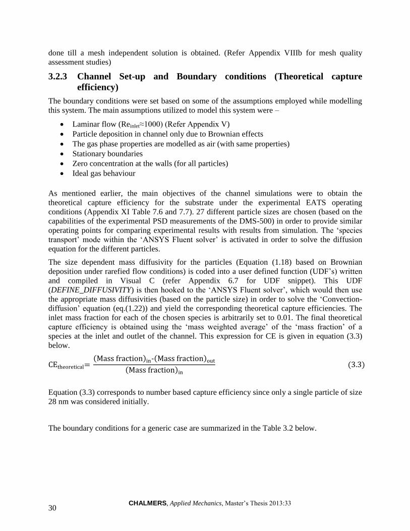
CHALMERS, Applied Mechanics, Master‘s Thesis 2013:33 30
done till a mesh independent solution is obtained. (Refer Appendix VIIIb for mesh quality
assessment studies)
3.2.3 Channel Set-up and Boundary conditions (Theoretical capture
efficiency)
The boundary conditions were set based on some of the assumptions employed while modelling
this system. The main assumptions utilized to model this system were –
Laminar flow (Reinlet≈1000) (Refer Appendix V)
Particle deposition in channel only due to Brownian effects
The gas phase properties are modelled as air (with same properties)
Stationary boundaries
Zero concentration at the walls (for all particles)
Ideal gas behaviour
As mentioned earlier, the main objectives of the channel simulations were to obtain the
theoretical capture efficiency for the substrate under the experimental EATS operating
conditions (Appendix XI Table 7.6 and 7.7). 27 different particle sizes are chosen (based on the
capabilities of the experimental PSD measurements of the DMS-500) in order to provide similar
operating points for comparing experimental results with results from simulation. The ‗species
transport‘ mode within the ‗ANSYS Fluent solver‘ is activated in order to solve the diffusion
equation for the different particles.
The size dependent mass diffusivity for the particles (Equation (1.18) based on Brownian
deposition under rarefied flow conditions) is coded into a user defined function (UDF‘s) written
and compiled in Visual C (refer Appendix 6.7 for UDF snippet). This UDF
(DEFINE_DIFFUSIVITY) is then hooked to the ‗ANSYS Fluent solver‘, which would then use
the appropriate mass diffusivities (based on the particle size) in order to solve the ‗Convection-
diffusion‘ equation (eq.(1.22)) and yield the corresponding theoretical capture efficiencies. The
inlet mass fraction for each of the chosen species is arbitrarily set to 0.01. The final theoretical
capture efficiency is obtained using the ‗mass weighted average‘ of the ‗mass fraction‘ of a
species at the inlet and outlet of the channel. This expression for CE is given in equation (3.3)
below.
Equation (3.3) corresponds to number based capture efficiency since only a single particle of size
28 nm was considered initially.
The boundary conditions for a generic case are summarized in the Table 3.2 below.

CHALMERS, Applied Mechanics, Master‘s Thesis 2013:33 31
The specific cases and their corresponding sub-cases that were studied in these simulations are
described below.
Channel under adiabatic conditions (at temperatures 150, 200 and 250°C and flow rates
of 150, 236 and 473 LPM)
Channel under non-adiabatic conditions with insulation (at a temperature of 250°C and a
flow rate of 150 LPM)
o Case a – Channel close to walls
o Case b – Channel quarter way from the walls
o Case c – Channel at the centre (half way from the walls)
Channel under non-adiabatic conditions without insulation (at a temperature of 250°C
and a flow rate of 150 LPM)
o Case a – Channel close to walls
o Case b – Channel quarter way from the walls
o Case c – Channel at the centre (half way from the walls)
For the adiabatic cases, the wall boundaries were set with zero heat flux (no heat loss in the
system). In order to model the non-adiabatic cases with and without insulation, an axial wall
temperature profile is applied. This temperature profile is obtained for the corresponding cases
from the 2-D axis-symmetric EATS simulations (for the experimental operating points Appendix
XI – table 7.6 and 7.7). Using this profile, a linear wall temperature function (temperature as a
function of z position) is generated (using the ‗polyfit2‘ function in MATLAB). This function is
then coded into a UDF (DEFINE_PROFILE). This UDF is then hooked to the ‗ANSYS Fluent
2‗ polyfit’ finds the coefficients of a polynomial p(x) of degree ‗n’ that fits the data, p(x(i)) to y(i), in a
least squares sense.
Velocity Inlet
Inlet Velocity 0.2 m/s, 0.3m/s or 0.6 m/s
Temperature 150, 200 or 250°C
Mass fraction of species at walls 0
Mass fraction of each species at inlet 0.01
Pressure outlet
Stationary wall
Table 3.2 – Generic boundary conditions for the channel simulations

CHALMERS, Applied Mechanics, Master‘s Thesis 2013:33 32
solver‘, and the corresponding temperature profile is set for the wall boundaries (refer Appendix
6.7 for UDF snippet). All the boundary conditions for these simulations are set based on the
experimental operating points (refer Appendix XI).
Figure 3.4 – Channel positions for the insulated and non-insulated cases
Case a
Case b
Case c
Figure 3.4 - Channel positions for the insulated and non-insulated cases

CHALMERS, Applied Mechanics, Master‘s Thesis 2013:33 33
4 Results and discussion
4.1 Results of the initial trials (1st & 2
nd sets)
4.1.1 Effect of concentration
The effect of concentration on particle size distribution for the 1st set of trials has been presented
in the Figure 4.1 below.
Figure 4.1 -The effect of concentration on PSD (1st set) at an upstream pressure of 3.5 bar
These specific trials (10, 24 and 43) from the 1st set of experiments have different concentrations
(10, 100 and 10000 ppm of sodium chloride solution) while the other inspected variables like
upstream pressure induced by the atomizer, dilution sets from the DMS and heating pipe
temperature were all kept the same. From the figure above, it is very evident that higher
concentration results in higher particle number concentrations (bigger area under the curve) with
a broader particle size range. The same trend was also observed in the 2nd
set of experiments for
trials (23, 26 and 29 see Figure 4.2 below)
Figure 4.2 - The effect of concentration on PSD (2nd set) at an upstream pressure of 2.5 bar
101
102
0
2
4
6
8x 10
7
Particle Size [nm]
Part
icle
num
ber
[dN
/dlo
g(d
P)]
Trial no 10 [10ppm]
Trial no 24 [100ppm]
Trial no 43 [10000ppm]
101
102
0
2
4
6
8x 10
7
Particle Size [nm]
Part
icle
num
ber
[dN
/dlo
g(d
P)]
Trial no 23 [5000ppm]
Trial no 26 [10000ppm]
Trial no 29 [15000ppm]
Trial 10
Trial 24
Trial 43
Trial 23
Trial 26 Trial 29

CHALMERS, Applied Mechanics, Master‘s Thesis 2013:33 34
4.1.2 Effect of the atomizer pressure (up-stream pressure) on PSD
Another important parameter that affected the particle size distribution was the pressure at the
atomizer (Pup). As specified earlier (Section 2.1.1), higher atomizer pressure yields higher flow
rates which results in higher particle number concentration. This is depicted in the Figure 4.3
below.
Figure 4.3 - The effect of atomizer pressure on PSD (2nd set) at a concentration of 10000ppm
These findings clearly indicate that higher concentrations and higher atomizer pressures yield
particle size distribution (range from 10 to 150 nm) and particle number concentration of 107
which is suitable in this study.
However, based on the current experimental observations, solution concentrations of higher than
10000 ppm were noted to clog the restrictor in DMS pipe system. In addition, upstream pressure
of more than 4 bar created severe instabilities in the atomizer. Thus, the concentration of 10000
ppm and Pup of 4 bar was chosen as the optimal condition to generate PM for the final sets of
experiments (the capture efficiency evaluation).
4.1.3 Particle size measurement evaluation
The total number of particles leaving the atomizer are subject to some difusion losses due to their
passage through several sections (heated pipe, DMS sampling tube and secondary diluter ). In
order to verify that the expressions employed in equation (2.3) account for the total diffusion
losses, a comprehensive evaluation of the obtained data was carried out. The calculation results
for PM diffusion losses in terms of penetration efficiencies for the heated pipe, DMS sampling
tube and the secondary diluter at the DMS for a chosen trial (no 43) from the 1
st sets of trials are
presented in the Figure 4.4.
101
102
0
2
4
6
8x 10
7
Particle Size [nm]
Part
icle
num
ber
[dN
/dlo
g(d
P)]
Trial no 25[Pup=1.5 bar]
Trial no 26[Pup=2.5 bar]
Trial no 27[Pup=3.5 bar]
Trial 25
Trial 26
Trial 27
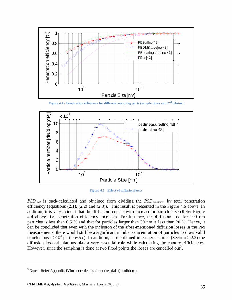
CHALMERS, Applied Mechanics, Master‘s Thesis 2013:33 35
Figure 4.4 - Penetration efficiency for different sampling parts (sample pipes and 2nd dilutor)
Figure 4.5 - Effect of diffusion losses
PSDreal is back-calculated and obtained from dividing the PSDmeasured by total penetration
efficiency (equations (2.1), (2.2) and (2.3)). This result is presented in the Figure 4.5 above. In
addition, it is very evident that the diffusion reduces with increase in particle size (Refer Figure
4.4 above) i.e. penetration efficiency increases. For instance, the diffusion loss for 100 nm
particles is less than 0.5 % and that for particles larger than 30 nm is less than 20 %. Hence, it
can be concluded that even with the inclusion of the afore-mentioned diffusion losses in the PM
measurements, there would still be a significant number concentration of particles to draw valid
conclusions ( >104 particles/cc). In addition, as mentioned in earlier sections (Section 2.2.2) the
diffusion loss calculations play a very essential role while calculating the capture efficiencies.
However, since the sampling is done at two fixed points the losses are cancelled out3.
3 Note – Refer Appendix IVfor more details about the trials (conditions).
101
102
0
0.2
0.4
0.6
0.8
1
Particle Size [nm]
Pe
ne
tra
tio
n e
ffic
ien
cy [%
]
PE2dil[no 43]
PEDMS tube[no 43]
PEheating pipe[no 43]
PEtot[43]
101
102
0
2
4
6
8
10
x 107
Particle Size [nm]
Part
icle
num
ber
[dN
/dlo
g(d
P)]
psdmeasured[no 43]
psdreal[no 43]

CHALMERS, Applied Mechanics, Master‘s Thesis 2013:33 36
4.2 Results from the initial simulations
This section describes the relevant results that have been obtained from the several numerical
analyses that were performed initially, i.e. the EATS and single channel simulations with
preliminary set-ups. The results from the EATS geometry are described in detail in the
following sections. It must be noted that, the results from the simulations is used to optimize the
experimental trials and would thus have a significant bearing on their outcome.
4.2.1 Results from the EATS simulations
Studies on the flow field within the EATS under two different geometrical configurations
(with and without the flow straighteners)
The effect of including the flow straightener in the EATS geometry was assessed. As explained
in the earlier sections (Section 3.1.1), the flow straightener serves the primary objective of
minimizing ‗re-circulation zone‘ effects. This would have an effect on the temperature profile
within the geometry. The vectors of velocity magnitude for two particular non-adiabatic cases
with insulation (250°C and 150 LPM - maximum heat losses) are compared in order to motivate
the inclusion of a flow straightener in the EATS geometry. The case with the flow straightener
would have hardly any recirculation effects (see figure below), thus there would be very poor
mixing within the fluid streams at the inlet of the substrate leading to a higher axial temperature
gradient along the EATS (412 to 523 K from the walls to the centre – refer figure 4.6 below) .
The case without the flow straightener, however would have much better mixing of the air
streams (due to recirculation) and would thus have a lower axial temperature gradient (503 to
523 K from the walls to the centre – refer figure 4.6 below). It is desired to have a temperature
gradient as low as possible at the inlet of the substrate in order to obtain as close to adiabatic
conditions within the substrate (which are the best operation conditions) as possible. Thus the
flow straightener clearly does not permit such conditions (due to the higher temperature
gradients it forms) and is hence removed from the EATS geometry.
Figure 4.6 - Contours of temperature for the case with a flow straightener (Top-left), Contours of velocity for the case
with a flow straightener (Top-right), Contours of temperature for the case without a flow straightener (Bottom-left) and
Contours of velocity for the case without a flow straightener (Bottom-right)

CHALMERS, Applied Mechanics, Master‘s Thesis 2013:33 37
4.2.2 Studies on the temperature profile within the EATS (without the flow
straighteners)
The energy equation is solved in the ‗ANSYS fluent solver‘ to give the requisite temperature
distribution within the EATS. These solutions are obtained on the basis of the inlet and wall
boundary conditions. These temperature profiles that were generated were utilized in order to
determine the most appropriate locations for placing the thermocouples in the substrate. These
thermocouples would provide real time temperature readings (while performing the capture
efficiency studies on the EATS) and would thus aid in maintaining as close to adiabatic
conditions as possible in the substrate (control the heater settings). In addition, as mentioned
earlier (Section 2.2.4)), a heating tape has been used in order to maintain the adiabatic conditions
within the substrate, the power to this tape would be controlled by a thermocouple which would
detect the temperature within the system and accordingly supply heat or shut off. This
thermocouple needs to be placed at the coldest possible region within the substrate (this is done
so as to compensate for the higher heat losses in this region). The EATS temperature profiles
generated from the CFD simulations were thus instrumental in determining the apt location to
place this thermocouple as well. The temperature contour for the EATS operating under non-
adiabatic conditions of 250°C and at a flow rate of 150 LPM, devoid of any insulation is shown
in the figure 4.7 below. These conditions would represent the worst operating conditions for the
EATS (maximum heat losses - due to higher temperatures and lower flow rates). An examination
of this plot would provide a good insight into the appropriate thermocouple placement locations
(Figure 4.7 below).
The Figure 4.7 below clearly indicates that, under these specific operating conditions, there is a
huge temperature gradient across the substrate (as expected). There is also a significant radial
temperature gradient (from the centre of the substrate to the walls) with the regions closest to the
wall colder than the centre by about 160°C. This would mean that, the coldest zones within the
substrate would be the regions closest to the walls. Thus the thermocouple controlling the
heating tape would have to be placed in the vicinity of this region. The additional thermocouples
which would provide real time information about the temperature within the substrates would
have to be placed in the following key locations (shown in the Figure below) in order to have a
measure of control over the adiabatic nature of the system.
Figure 4.7 – Contours coloured by temperature (over the substrate) overlaid with a thermocouple map (based on a
substrate at 250°C (at the point ‘substrate begin’), 473 LPM and No insulation)
CHALMERS, Applied Mechanics, Master‘s Thesis 2013:33 38
Ten thermocouples were available in total, out of these; two were needed to monitor the heater
outlet and the pre-substrate region respectively. The remaining 8 thermocouples were placed in
the locations within the substrate as shown in the map above. Thermocouples 2, 3 and 1 were
placed 2.5 cm away from the beginning of the substrate; thermocouples 5 and 6 were placed 7.5
cm away from the beginning of the substrate and thermocouples 7, 8 and 9 were placed 12.5 cm
from away from the beginning of the substrate. The axial positions of the thermocouples are as
follows – 2, 5 and 8 were placed 0.5 cm away from the wall; 3, 6 and 9 were placed 3.5 cm away
from the walls and 1 and 7 were placed at the centre of the substrate (7.5 cm away from the
walls). The thermocouple controlling the heating tape (12) was placed closed to the walls (near
the insulation mat at the rear end of the substrate) so that it would compensate for the heat losses
and accordingly regulate the power supplied to the heating tape. A photograph of the actual
thermocouple placement within the substrate is also shown in the Figure 4.7.
The temperature profile within the catalyst at 250°C (523K) under two different flow rates (150
LPM and 473 LPM) was also assessed. The simulations clearly demonstrate the effect of
increased flow rate on the temperature profile developed within the substrate (see figure 4.8
below). The shorter residence time (higher flow rate – 473 LPM) would mean that the fluid has
lesser time to transfer heat to its surroundings (lesser heat losses). This would mean that there
would be a lower temperature gradient developed within the substrate (as demonstrated in the
figure below). The lower flow rate, on the other hand would mean that there would be higher
heat loses from the flow (longer residence time) leading to a larger temperature gradient within
the substrate. This fundamental concept of residence time and temperature gradient development
in a non-adiabatic system would have a significant bearing on the capture efficiency of the
substrate. The CFD simulations thus provide a very good insight into the overall flow conditions
aiding in preparing and performing better experimental trials. (Refer Appendix IX for
comparison between temperature profiles obtained in experiments and simulations)
Figure 4.8 – Effect of flow rate on the temperature profile across the catalyst (at 250 °C)
0.35 0.4 0.45 0.5500
505
510
515
520
525
530
Position [m]
Te
mp
era
ture
[°C
]
150 LPM
473 LPM

CHALMERS, Applied Mechanics, Master‘s Thesis 2013:33 39
4.3 Experimental CE trials
The effects of different experimental conditions on capture efficiency have been assessed and
some specific cases are presented in the following sections (the rest are presented in the
Appendix XII and XIII). Subsequently, these specific cases are compared to make the final
conclusions. These cases are-
Case A – Substrate under non-adiabatic conditions with insulation
o Case A1-Effect of residence time at the highest temperature (150, 236 and 473
LPM at 250°C)
o Case A2 - Effect of temperature at the lowest flow rate (150, 200 and 250°C at
150 LPM )
Case B – Substrate under adiabatic conditions
o Case B1 – Effect of residence time at the highest temperature (150, 236 and 473
LPM at 250°C)
o Case B2– Effect of temperature at the lowest flow rate (150, 200 and 250°C at
266 LPM)
Cases C- The comparison between adiabatic and non-adiabatic capture efficiencies (case
A & B)
o Case C1- Both cases are assessed at the highest temperature of 250°C and lowest
flow rate of 150 LPM
o Case C2 - Both cases are assessed at the lowest temperature of 150°C and highest
flow rate of 473 LPM
4.3.1 Capture efficiency for the non-adiabatic conditions (Case A)
Effect of residence time (Case A1)
In this set of experiments, the inlet temperature at the substrate was fixed and maintained at
250°C. Three different volumetric flow rates of 150, 236 and 473 LPM were chosen to evaluate
the effect of residence time on capture efficiency. The red, blue and black lines correspond to
experiment number 20, 23 and 26 respectively.
Figure 4.9 - Effect of residence time on capture efficiency at 250°C (Experiment no 20, 150 LPM, Channel Re = 5.61, Sh
(at 27nm) = 8.06 and CE (at 27 nm) = 25.65 %), (Experiment no 23, 236 LPM, Channel Re = 8.11, Sh (at 27nm)=9.75 and
CE (at 27 nm) = 21.27 %),( Experiment no 26, 473 LPM, Channel Re=15.13, Sh (at 27nm) = 13.09 and CE (at 27 nm) =
15.55 %)
From the Figure above (4.9), it is very evident that the capture efficiency increases with increase
in residence time. The rate of increase in capture efficiency for a reduction in flow rate from 236
101
102
0
20
40
60
80
100
Particle Size [nm]
Ca
ptu
re e
ffici
en
cy [%
]
150 LPM[250 deg C]
236 LPM[250 deg C]
473 LPM[250 deg C]
150 LPM
236 LPM
473 LPM
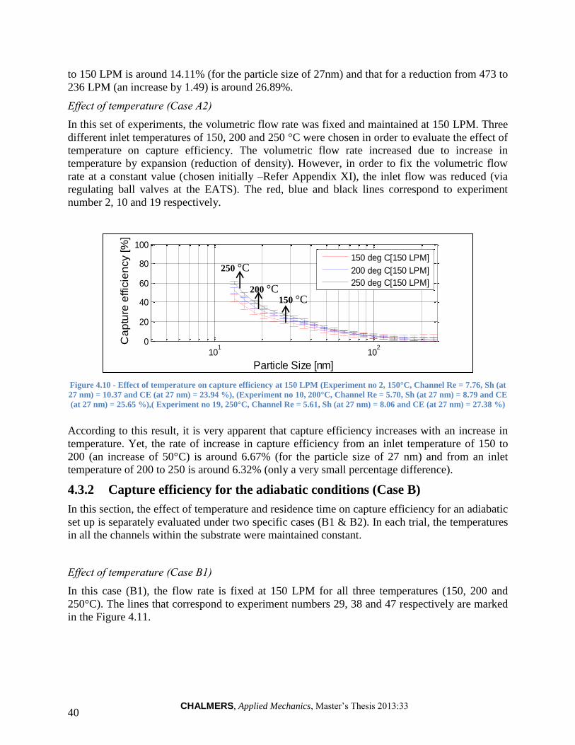
CHALMERS, Applied Mechanics, Master‘s Thesis 2013:33 40
to 150 LPM is around 14.11% (for the particle size of 27nm) and that for a reduction from 473 to
236 LPM (an increase by 1.49) is around 26.89%.
Effect of temperature (Case A2)
In this set of experiments, the volumetric flow rate was fixed and maintained at 150 LPM. Three
different inlet temperatures of 150, 200 and 250 °C were chosen in order to evaluate the effect of
temperature on capture efficiency. The volumetric flow rate increased due to increase in
temperature by expansion (reduction of density). However, in order to fix the volumetric flow
rate at a constant value (chosen initially –Refer Appendix XI), the inlet flow was reduced (via
regulating ball valves at the EATS). The red, blue and black lines correspond to experiment
number 2, 10 and 19 respectively.
Figure 4.10 - Effect of temperature on capture efficiency at 150 LPM (Experiment no 2, 150°C, Channel Re = 7.76, Sh (at
27 nm) = 10.37 and CE (at 27 nm) = 23.94 %), (Experiment no 10, 200°C, Channel Re = 5.70, Sh (at 27 nm) = 8.79 and CE
(at 27 nm) = 25.65 %),( Experiment no 19, 250°C, Channel Re = 5.61, Sh (at 27 nm) = 8.06 and CE (at 27 nm) = 27.38 %)
According to this result, it is very apparent that capture efficiency increases with an increase in
temperature. Yet, the rate of increase in capture efficiency from an inlet temperature of 150 to
200 (an increase of 50°C) is around 6.67% (for the particle size of 27 nm) and from an inlet
temperature of 200 to 250 is around 6.32% (only a very small percentage difference).
4.3.2 Capture efficiency for the adiabatic conditions (Case B)
In this section, the effect of temperature and residence time on capture efficiency for an adiabatic
set up is separately evaluated under two specific cases (B1 & B2). In each trial, the temperatures
in all the channels within the substrate were maintained constant.
Effect of temperature (Case B1)
In this case (B1), the flow rate is fixed at 150 LPM for all three temperatures (150, 200 and
250°C). The lines that correspond to experiment numbers 29, 38 and 47 respectively are marked
in the Figure 4.11.
101
102
0
20
40
60
80
100
Particle Size [nm]
Ca
ptu
re e
ffic
ien
cy [%
]
150 deg C[150 LPM]
200 deg C[150 LPM]
250 deg C[150 LPM]
250 °C
200 °C
150 °C

CHALMERS, Applied Mechanics, Master‘s Thesis 2013:33 41
Figure 4.11 - Effect of residence time on capture efficiency at 150°C, adiabatic (Experiment no 29 , 150 LPM, Channel
Re = 7.78, Sh (at 27 nm) = 10.37 and CE (at 27 nm) = 25.87 %), (Experiment no 38, 236 LPM, Channel Re = 12.36, Sh (at
27 nm) =17.10 and CE(at 27 nm)=18.51 %),( Experiment no 47, 473 LPM, Channel Re = 24.65, Sh (at 27 nm) = 17.10 and
CE (at 27 nm) = 14.41 %)
The effect of residence time on capture efficiency follows the same trend as presented in the non-
adiabatic cases (reduction in residence time would increase the capture efficiency and vice
versa.)
Effect of residence time (Case B2)
The lines that correspond to experiment numbers 48, 51 and 51 respectively are represented in
the Figure 4.12 below.
Figure 4.12- Effect of temperature on capture efficiency at 473 LPM, adiabatic case (Experiment no 48, 150°C, Channel
Re = 24.65, Sh (at 27 nm) = 17.10 and CE (at 27 nm) = 14.41 %), (Experiment no 51, 200°C, Channel Re = 16.95, Sh (at
27 nm) = 14.36 and CE (at 27 nm) = 19.04 %),( Experiment no 54, 250°C, Channel Re = 15.49, Sh (at 27 nm) = 13.09 and
CE (at 27 nm) = 22.99 %)
The results from cases B1 and B2 further confirm the trends noticed in the non-adiabatic trials
(Case A1 and A2) in the sense that effect of residence time is higher than effect of temperature
e.g. the capture efficiency results obtained from two cases (A1 & A2) showed that an increase of
100°C in temperature results in a 12.56 % increase in capture efficiency while a decrease of 86
LPM (increase in residence time) still results in a higher capture efficiency increase of 14.11 %.
Therefore, it is very evident that residence time has a higher effect on capture efficiency
compared to temperature. This finding is also explained by the correlations presented in (Johnson
& Kittelson, 1996)(eq : (1.19), (1.20), (1.21) and (1.22)) where, capture efficiency is
exponentially related to the average mass transfer coefficient (hm) and residence time. This
coefficient (hm) increases due to increase in temperature leading to an increase in deposition
101
102
0
20
40
60
80
100
Particle Size [nm]
Ca
ptu
re e
ffic
ien
cy [%
]
150 Deg C[150LPM]
200 Deg C[150LPM]
250 Deg C[150LPM]
101
102
0
20
40
60
80
100
Particle Size [nm]
Ca
ptu
re e
ffici
en
cy [%
]
150 LPM[250 Deg C]
236 LPM[250 Deg C]
473 LPM[250 Deg C]
250 °C
200 °C
150 °C
150 LPM
236 LPM
473 LPM

CHALMERS, Applied Mechanics, Master‘s Thesis 2013:33 42
efficiency. Therefore it can be concluded that temperature has a secondary effect and residence
time has a direct effect on capture efficiency.
4.3.3 Comparison between non-adiabatic and adiabatic conditions (Case C)
High residence time & high temperature (Case C1)
The capture efficiency of different cases with the same flow but under different conditions
(adiabatic & non-adiabatic) was evaluated. Two specific cases are presented in this section (The
rest are presented in Appendix XIV). Based on the results from the previous cases, low flow rate
(high residence time) and high temperature scenarios were chosen in order to produce the highest
capture efficiencies. The results are presented in the Figure 4.13 below. The adiabatic and non-
adiabatic curves correspond to trial numbers 47 and 26 respectively.
Figure 4.13 - Experiment no 47 at 250°C and 150 LPM, Channel Re =4.47, Sh (at 27 nm) = 8.06 and CE (at 27 nm) =
39.21 %, The experiment no 26, the non-adiabatic conditions at 250°C and 150 LPM, Channel Re = 5.61, Sh (at 27 nm) =
8.06 and CE (at 27 nm) = 25.65 %
The higher capture efficiency of the adiabatic case is due to its higher average channel
temperature (most channels were kept at 250°C). In the non-adiabatic case however, the average
temperature is lower as channels closest to the periphery of the substrate are at temperatures
lower than 250°C (due to un-compensated heat losses to the surrounding) thereby leading to a
lower capture efficiency.
Low residence time & low temperature (Case C2)
In Figure 4.14, the adiabatic and non-adiabatic curves correspond to experiment numbers 35 and
8 respectively. However, it is very apparent (similar to the pervious case (C1)) that the adiabatic
set up has the higher capture efficiency. Furthermore, the difference between the two CEs is
much lesser than the trend noticed in the previous case (C1).This could be due to the high flow
rate (low residence time) and low temperature that reduces the heat loss (lower temperature
gradient - Section 4.2.2) increasing the average substrate temperature in the non-adiabatic case.
This means that both set ups (adiabatic and non-adiabatic in case (C2)) have very close average
temperatures. Moreover, since the residence for both cases were kept the same, they showed very
close capture efficiency profiles. The radial temperature gradient for non-adiabatic condition in
both cases (C1 & C2) was also calculated by using CFD to validate this finding (refer Appendix
XV).
101
102
0
20
40
60
80
100
Particle Size [nm]
Ca
ptu
re e
fficie
ncy
[%]
Adiabatic,250 deg C[150 LPM]
Non-adiabatic,250 deg C[150 LPM]
Adiabatic
Non-adiabatic

CHALMERS, Applied Mechanics, Master‘s Thesis 2013:33 43
Figure 4.14 - Experiment no 35, adiabatic at 150°C and 473 LPM, Channel Re = 24.65, Sh (at 27 nm) = 17.10 and CE (at
27 nm) = 14.41 %. The non-adiabatic conditions experiment no 8 at 150°C and 473 LPM, Channel Re = 24.16, Sh (at 27
nm) = 17.10 and CE (at 27 nm) = 13.29 %
4.4 Results from single channel capture efficiency simulations
(theoretical CE)
The channel simulations were the primary tool to establish the theoretical capture efficiencies.
These simulations thus provided a valuable insight into the capture phenomenon within open
substrates. The channel was studied under two conditions – non-adiabatic and adiabatic (in a
similar manner as detailed in the section on experimental capture efficiency trials Section 4.2).
There were two primary effects assessed in these simulations, these were-
Effect of temperature
Effect of residence time
4.4.1 Adiabatic channel simulations
The effect of residence time was studied by comparing simulations that had the same operating
temperature but differ in flow rates (150 LPM, 236 LPM and 473 LPM). The result of increasing
flow rates at constant temperatures of 150 and 250°C are shown in the figure below (Figure
4.15). The theoretical CE reduces with increasing flow rates. This trend is very similar to the one
observed while doing experimental trials. As elucidated in the previous sections, increasing the
flow rate reduces the residence time of the inert particulates in the monolith channel. The
residence time is inversely correlated with the Brownian deposition (as explained in Section
4.3.1), resulting in the observed trend.
101
102
0
20
40
60
80
100
Particle Size [nm]
Ca
ptu
re e
ffic
ien
cy [%
]
Adiabatic,150 deg C[473 LPM]
Non-adiabatic,150 deg C[473 LPM]
Adiabatic Non-adiabatic

CHALMERS, Applied Mechanics, Master‘s Thesis 2013:33 44
Figure 4.15 – Effect of flow rate on theoretical capture efficiency at a constant temperature of 250°C (left) and 150°C
(right)
The effect of temperature on capture efficiency was studied by comparing simulations that had
the same operating flow rates of 150 LPM and 437 LPM but differ in temperature (150°C, 200°C
and 250°C).
The figure below clearly demonstrates the trend that increasing temperatures increases the
capture efficiency. This is primarily attributed to the reduction in diffusivity (within the channel)
as we all as corresponding increase in diffusivity of the particles at higher temperatures (as
explained in Section 4.3.1).
Figure 4.16 – Effect of temperature on theoretical capture efficiency at constant flow rate of 150 LPM (left) and at
constant flow rate of 473 LPM (right)
Figures 4.15 and 4.16 clearly indicate the general trend that the residence time (flow rate) brings
about a greater spread in CE than the temperature. This trend is discussed more in detail in
section 4.3.3.
101
102
0
20
40
60
80
100
Particle Size [nm]
Ca
ptu
re e
ffic
ien
cy [%
]
Q = 150 LPM
Q = 236 LPM
Q = 473 LPM
101
102
0
20
40
60
80
100
Particle Size [nm]
Ca
ptu
re e
ffic
ien
cy [%
]
Q = 150 LPM
Q = 236 LPM
Q = 473 LPM
101
102
0
50
100
Particle Size [nm]
Ca
ptu
re e
ffic
ien
cy [%
]
T = 150°C
T = 200°C
T = 250°C
101
102
0
50
100
Particle Size [nm]
Ca
ptu
re e
ffic
ien
cy [%
]
T = 150°C
T = 200°C
T = 250°C
150 LPM
236 LPM
473 LPM 473 LPM
236 LPM
150 LPM
150 °C 200 °C
250 °C
150 °C 200 °C
250 °C

CHALMERS, Applied Mechanics, Master‘s Thesis 2013:33 45
4.4.2 Non-Adiabatic channel simulations
Channel in an insulated substrate
Figure 4.17 – Effect of channel location on theoretical capture efficiency at constant flow rate of about 150 LPM and
250°C – channels in an insulated substrate (left), Axial temperature profile along the channel (right)
The non-adiabatic channel simulations give an insight into the impact of an external temperature
gradient (along the channel) on the variation in capture efficiency. The channel studied in a
substrate with insulation demonstrated a very important trend with respect to location of the
channel within the substrate. As mentioned earlier (section 3.2.3 Figure 3.3), three different
channel positions were simulated i.e., Case a – Channel close to walls, Case b – Channel 0.5 r
away from the walls and Case c – Channel at the centre, at the same flow rate and inlet
temperature in the EATS (250 °C and 150 LPM) . The axial temperature profiles (Figure 4.17
(right)) clearly show that the temperature gradient in the channels close to the walls is much
steeper (from about 230 to 220°C) than the corresponding gradients in the channels at quarter
distance from the walls (from about 247 to 242°C) and the channels at the centre (from about
250 to 248°C). Thus, the CE‘s vary as well, with the channel in the centre (Case c) having the
highest CE when compared to the CE‘s at the other two positions. However, the similar gradients
in temperature between cases b and c entails that the corresponding difference in CE between
these two cases must be almost negligible (change in an absolute magnitude of 10°C in
temperature would not bring about such a drastic difference in CE) as shown clearly in the
Figure 4.17 above. Moreover, there is no drastic difference in the CE between the three cases,
indicating that the insulation being employed is able to maintain as close to adiabatic conditions
possible. Thus, if the EATS is operated even without the heating tape (section 2.2.4), the
temperature conditions that could prevail within the substrate would ensure that there are no
large differences in CE between channels located in the periphery of the substrate and the centre.
Channels in a non-insulated substrate
The channels studied in a non-insulated substrate under the same EATS operating conditions
(250°C and 150 LPM, the worst possible operating conditions) also demonstrated the similar
trend as in the channels in an insulated substrate. The main difference between the two operating
conditions (insulated and non-insulated) would be that, the cases a, b and c have successively
and clearly decipherable change in CEs with the channel in the centre (Case c) .The CE
dispersion with temperature variation this time is more apparent even between cases b and c.
101
102
0
20
40
60
80
100
Particle Size [nm]
Ca
ptu
re e
ffic
ien
cy [%
]
Case a
Case b
Case c
0.35 0.4 0.45 0.5220
230
240
250
Axial distance along the channel [m]
Te
mp
era
ture
[°C
]
Case a
Case b
Case cCase a
Case b
Case c
Case a Case b
Case c

CHALMERS, Applied Mechanics, Master‘s Thesis 2013:33 46
Figure 4.18 – Effect of channel location on theoretical capture efficiency at constant flow rate of about 150 LPM and
250°C – channels in a non-insulated substrate (left), Axial temperature profile along the channel (right)
The axial temperature profiles (Figure 4.18 (right)) are more pronounced in these non-insulated
cases (higher heat loss to the surroundings) with the temperature gradient in the channels close to
the walls much steeper (from about 150 to 100°C) than the corresponding gradients in the
channels at quarter distance from the walls (from about 228 to 198°C) and the channels at the
centre (from about 248 to 227°C). Thus, the CEs vary as well, with the channel in the centre
(Case c) having the highest CE when compared to the CEs at the other two positions.
These two non-adiabatic channel simulations clearly indicate that, insulation of the substrate
does play a vital role in the CE measured across it. Clearly, on using insulated substrates, there
are no marked changes in the CE along channels located at different locations within the channel
(case a, b and c). This would mean that a mixed cup sampling probe (as employed to sample the
exhaust leaving the substrate in this work – Section 2.2.4) would give a reasonably accurate
estimate of the CE across the substrate (as long as the system is insulated). No additional work
would need to be done by varying the sampling probe types (to say localized probe samplers
such as sampling done very close to wall or sampling close to the centre etc.) as the simulations
clearly depict that there would be no apparent effect on CE due to these variations.
4.4.3 Results from the Johnson and Kittleson correlations
Both EATS and ingle channel simulations performed were based on the correlations presented in
Kittleson et.al (1996). Some simple results were obtained by using these correlations directly.
The results from these correlations have been compared with the CFD simulations as well
(showing good agreement – refer Appendix XIX). Thus, by directly employing the correlations,
exact effects of residence time and temperature can be assessed under fictitious conditions, i.e.
operational conditions that cannot be physically achieved in a real system. The only objective of
these studies was to provide a pedagogical backing for the results obtained in the simulations and
experimental trials.
A ‗pseudo-fluid (air with fictitious properties)‘, was studied under the following 5 cases –
Case A – Base case at 200°C (viscosity and density based on temperature of 200°C)
Case B – Pseudo-fluid 1 (constant viscosity fluid) at 150°C (density based on temperature
of 150°C and viscosity based on temperature of 200°C)
Case C – Pseudo-fluid 1 at 250°C (density based on temperature of 250°C and viscosity
based on temperature of 200°C)
101
102
0
50
100
Particle Size [nm]
Ca
ptu
re e
ffic
ien
cy [%
]
Case a
Case b
Case c
0.35 0.4 0.45 0.5100
150
200
250
Axial distance along the channel [m]
Te
mp
era
ture
[°C
]
Case a
Case b
Case cCase a
Case b
Case c
Case a Case b
Case c

CHALMERS, Applied Mechanics, Master‘s Thesis 2013:33 47
Case D – Pseudo-fluid 2 (constant density fluid) at 150°C (density based on temperature
of 200°C and Viscosity based on temperature of 150°C)
Case E – Pseudo-fluid 2 at 250°C (density based on temperature of 200°C and Viscosity
based on temperature of 250°C)
In this fictitious set-up, the aim of employing a constant viscosity fluid (Pseudo-fluid 1) was to
demonstrate the effect of residence time separately at constant particle diffusivities. Hence, the
decrease in density of pseudo-fluid 1 on increase in temperature is attributed to decrease in
residence time. It must be noted that the velocity of the pseudo-fluid (both 1 and 2) is constant
(at 0.2 m/s which corresponds to the 150 LPM flow) in all the cases studied. The constant
density fluid (pseudo-fluid 2) on the other hand, would be used to demonstrate the effect of
temperature (diffusion coefficient of the particle) at constant residence times.
The Figure 4.17 depicts the results from this simple study. The Case A forms a reference line
(blue line) to which the other cases are compared. The Cases B and C (magenta and black lines),
which demonstrate the effect of residence time, clearly confirm the trend observed in the
experimental as well simulation results. There is a marked decrease in capture efficiency as the
residence time increases. This can be seen by reformulating equation (1.19) in the following
manner –
Q
AhCE sm
channel exp1
(1.19)
U
4ShDLexp1CE
2channel
hd (4.1)
By employing the pseudo-fluid 1 at constant velocities, equation (4.1) can be re-written as -
(4.2)
Where ‗τ ‗is the residence time. Thus, there is an exponential relation between theoretical capture
efficiency and residence time. ‗C‘ is synonymous with ‗hm‘ (Equation (1.17)).Hence, on
increasing residence time, capture efficiency increases and the opposite is observed on
decreasing residence time.
The effect of temperature at constant residence time can be demonstrated by studying cases D
and E (red and green lines). As the temperature is increased the molecular momentum transfer
rate increases further which increases the viscosity of the gas. Moreover, at higher temperatures,
the diffusion coefficient increases (refer equation (1.22)). The overall effect of these two
parallelly acting influences would be an increase in capture efficiency from Case D to Case E as
the temperature is increased (demonstrated in Figure 4.17)
Among these two factors, i.e., the residence time and the temperature, the effect of residence
time is slightly more pronounced. This can be attributed to the direct exponential dependence of
CE on τ (equation (4.2)). The effect of temperature is however slightly less pronounced, this can
be attributed to the fact that temperature affects the CE indirectly via the Sherwood number and
C exp1CEchannel

CHALMERS, Applied Mechanics, Master‘s Thesis 2013:33 48
diffusivity. Moreover, as the effect of temperature is by no means negligible. In conclusion, both
temperature and residence time have a significant impact on the capture efficiency due to
Brownian deposition along a monolith channel.
Figure 4.17 – Pseudo-fluid studies
4.5 Comparison between experiments and simulations
The primary objective of this work was to establish congruence between experimental trials and
simulations for an inert particulate matter. Thus, the experimental results obtained (in Section
4.3) were compared with the corresponding simulations (in Section 4.4). It must be noted here
that the conditions employed in the channel simulations mimicked closely the experimental
operating conditions. Hence, any comparison between the two would represent a viable
association between theory and experiments.
4.5.1 Comparison under adiabatic conditions
The monolith channel under adiabatic operation would represent the most ideal condition in a
substrate. This was one of the primary reasons as to why these conditions have been discussed
extensively in the earlier sections (Sections 4.2 and 4.3). Comparisons are thus made between
the experiments and simulations at adiabatic conditions in order to verify that PM capture of
inert particulate matter can indeed be modelled and simulated utilizing CFD. The CE obtained
from the simulations at 150°C and at flow rates of 150 LPM and 436 LPM are compared with
the corresponding experiments (Experiment No 29 and 36 in Appendix XI Table 7.6). These
results are presented in the Figures 4.18.
101
102
20
40
60
80
Particle Size [nm]
Captu
re e
ffic
iency [%
]
Case A - Base case - 200°C
Case B –Pseudo-f luid 1 at 150°C(µ = µ(200 °C))
Case C – Pseudo-f luid 1 at 250°C(µ = µ(200 °C))
Case D - Pseudo-f luid 2 at 150°C(rho =rho(200 °C))
Case E - Pseudo-f luid 2 at 250°C(rho =rho(200 °C))

CHALMERS, Applied Mechanics, Master‘s Thesis 2013:33 49
Figure 4.18 - Comparison of CE obtained from experiments and simulations at 150°C, 150 LPM (left) and 150°C, 473
LPM (right)
These figures clearly demonstrate the congruence between simulations and experiments. The CE
from simulations fall within the error bars in the experimentally determined CE‘s indicating a
strong agreement between the two. The same trend is also observed in almost all the adiabatic
experimental operating points (refer Appendix XVIa).
4.5.2 Comparison under non-adiabatic conditions
Figure 4.19 - Comparison of CE obtained from experiments and simulations (channel at the centre) at 250°C, 150 LPM
The comparison between experiments and simulations under non-adiabatic conditions also
revealed a good agreement between theoretical and experimental findings. The above figure
compares the simulation results from a channel at the centre with experimental CE‘s, at 250°C
and 150 LPM. The same congruence is also observed when the channels at the other two
positions (close to walls and quarter distance from the walls) are compared with the experimental
findings (Refer Appendix XVIb). This further affirms the fact that the sampling methodology
chosen in the experiments are able to measure the substrate CE accurately. However, it must be
noted that, the experimental CE for smaller particle sizes (values determined from measurement
at the DMS500) reaches 100 % as the signal (in these cases) gets below the limit of detection of
the instrument, thus the value that gets measured at this size (for PSD) is zero.
101
102
0
20
40
60
80
100
Particle Size [nm]
Ca
ptu
re E
ffic
ien
cy ±
err
or
[%]
CE from experiments
CE from simulations
101
102
0
20
40
60
80
100
Particle Size [nm]
Ca
ptu
re E
ffic
ien
cy ±
err
or
[%]
CE from experiments
CE from simulations
101
102
0
20
40
60
80
100
Particle Size [nm]
Ca
ptu
re E
ffic
ien
cy ±
err
or
[%]
CE from experiments
CE from simulations

CHALMERS, Applied Mechanics, Master‘s Thesis 2013:33 50

CHALMERS, Applied Mechanics, Master‘s Thesis 2013:33 51
5 Conclusions and recommendations
This section describes the final conclusions of this work. These are based on the initial objectives
that were established before the start of this work. They are as follows -
5.1 Conclusions
1. Developed a methodology to generate inert PM at the desirable size and number
concentration: Sodium chloride aerosols (inert) with the constant particle size
distributions were produced from their aqueous solution by using the TOPAS ATM230
aerosol generator. The optimal solution concentration (10000 ppm) and atomizer
operation pressure (4 bar) in order to produce a desirable size range (10-150 nm) and
statistically significant number concentration of PM (>104
particles/cc - low signal to
noise ratio at the DMS) were also obtained. The desirable size and number concentration
range chosen in this study were able to draw close parallelisms with actual particulate
matter emitted from engines. Therefore, it is possible to generate and measure inert PM
using the set up described in this study (section 2.2).
2. Identified appropriate operating conditions while performing studies on open substrates
in order to examine the CE of inert PM: The chosen experimental operating points (while
performing experiments on the EATS) aided in evaluating specific trends pertaining to
the capture efficiency of inert particulate matter in an open substrate. The operating flows
of 150, 276 and 473 LPM are significantly lower than the nominal engine exhaust flows
(about 7080, 12035 and 16990 LPM), however at these low flows, the channel capture
efficiencies can be studied more in detail, i.e. trends are easily identified (due to higher
capture efficiencies that are measured). (Refer Appendix XVII for detailed sensitivity
analyses of CE at nominal engine operations). The chosen temperatures of 150, 200 and
250°C represent approximately the lower and upper boundaries of an operational
monolith (in an automotive application) under standard conditions.
3. Developed a methodology to combine CFD evaluations with experiments: A strong
interdependency between numerical simulations and experimental trials has been
demonstrated throughout this work. CFD evaluations have been used as a basis to plan
and perform better experiments. The complete 2D-axis symmetric evaluation of the
EATS (done prior to the experimental evaluation) assisted in optimizing the EATS pilot
set-up in the lab (by the removal of the flow straightener sections), enabling the
development of a more uniform temperature distribution at the substrate. Moreover, the
thermal profiles of the substrate generated from the simulations aided in establishing a
thermocouple map, providing the apt locations to place the temperature probes, in order
to monitor the substrate and maintain it at adiabatic conditions (the real time
measurements from the temperature probes determined the power supply to the heater
and the heating tape used to maintain the set temperature in the EATS). The temperature
profiles generated from the EATS simulations without any insulation i.e. at the worst
operating conditions (150 LPM and 250°C) also gave a valuable insight into the
insulation requirements of the EATS.
4. Accuracy and validity of the simulations: The primary argument towards any simulation
driven approach to examine a phenomenon, is the accuracy and validity of the results
obtained. This validity of the set-up is established by comparing the simulation results

CHALMERS, Applied Mechanics, Master‘s Thesis 2013:33 52
with results from corresponding experiments and or theoretical approximations
(empirical correlations, such as Equation (1.17)). A good congruence between
experimental results and simulations (Section 4.4) has been demonstrated throughout this
work. In addition, the simulations when compared to theoretical correlations, slightly
under predict the results (which should be the case). These two comparisons validate the
numerical set-up proposed in this work (Refer Appendix XIX).
5. Demonstrated the congruence between simulation and experiments for capture of inert
PM in open substrates: One of the primary objectives of this work was to evaluate the
congruence between numerical simulations and experimental results. This congruence is
evident throughout this work, with the simulations corresponding with the experimental
results (simulations results are within the error limit of the experimental results as
discussed in section 4.4 and in Appendix XVI). In addition the general trends with
variation in residence time (flow conditions) and temperature are noticeably similar in
both experiments and simulations. This indicates that the theory behind the description of
capture efficiency in monolith channels (Brownian deposition) is able to explain the
capture phenomena of inert particulates accurately. Moreover, this work also
demonstrated the congruence between CFD and theory (Appendix XIX) and further
validated the accuracy of the simulations. Thus, CFD analysis can be used when
correlations from literature are not sufficient (particularly when there is a temperature or
velocity gradient within the channel) to predict the capture efficiency of inert particulates
in open substrates.
6. Developed a methodology to evaluate the effect of residence time and temperature
(individually) on the CE of inert PM in open substrates. This work extensively described
the capture efficiency of inert particulate matter (sodium chloride) in open substrates. The
effect of different flow (mainly temperature and residence time) and operating conditions
(adiabatic and non-adiabatic) were comprehensively investigated by means of both
experimental trials and numerical simulations. As explained in the earlier sections
(section 4.3.2), the expected capture efficiency variation trends were; increase in
residence time and temperature increased the CE with the residence time having the
slightly more dominant effect. Both experimental and numerical results have confirmed
this trend.
5.2 Recommendations and future work
1. An alternate inert particulate matter system such as PSL (polystyrene) suspension of
specific diameters should be evaluated in order to confirm the trends observed in this
work.
2. This work should be advanced to the next level of complexity by performing experiments
with material closer to engine particulates such as artificial soot in the form of ‗Printex
U‘ (carbon black pigment used in printers). Some reactive phenomena of the PM could
be studied using this material.
3. The work on the substrate should be extended towards actual test bench studies, i.e. using
the DOC, DPF and SCR after treatments in series in order to study the overall efficiency
of the after-treatment system.

CHALMERS, Applied Mechanics, Master‘s Thesis 2013:33 53
4. The simulations of CE in the channels must be extended towards reactive PM (including
evaporation and mass transfer laws).

CHALMERS, Applied Mechanics, Master‘s Thesis 2013:33 54

CHALMERS, Applied Mechanics, Master‘s Thesis 2013:33 55
6 References
Adler, J. (2005). Ceramic Diesel Particulate Filters. International Journal of Applied Ceramic
Technology, 2(6), 429-439. doi: 10.1111/j.1744-7402.2005.02044.x
Allen, M. D., & Raabe, O. G. (1982). Re-evaluation of millikan's oil drop data for the motion of
small particles in air. Journal of Aerosol Science, 13(6), 537-547. doi:
http://dx.doi.org/10.1016/0021-8502(82)90019-2
Balkanski, Y., Myhre, G., Gauss, M., Radel, G., Highwood, E. J., & Shine, K. P. (2010). Direct
radiative effect of aerosols emitted by transport from road, shipping and aviation.
Atmospheric Chemistry and Physics, 10(10), 4477-4489.
Carmichael, G. R. (1982). Estimation of the drag coefficient of regularly shaped particles in slow
flows from morphological descriptors. Industrial & Engineering Chemistry Process
Design and Development, 21(3), 401-403. doi: 10.1021/i200018a009
Chandrasekhar, S. (1943). Stochastic Problems in Physics and Astronomy. Reviews of Modern
Physics, 15(1), 1-89.
Cox, P. M., Betts, R. A., Jones, C. D., Spall, S. A., & Totterdell, I. J. (2000). Acceleration of
global warming due to carbon-cycle feedbacks in a coupled climate model. Nature (408),
184-187.
Creaser, D. (2013). Coursework in advanced chemical reaction engineering. Chalmers
Univertsity of Technology, Department of chemical engineering.
Crowe, C. T., Schwarzkopf, J. D., Sommerfeld, M., & Tsuji, Y. (2011). Multiphase flows with
droplets and particles. CRC Press, Second edition.
Daley, D. J., & Vere-Jones, D. (1988). An Introduction to the Theory of Point Processes.
Springer–Verlag, New York.
Donaldson. (2009). Calculating engine airflow. Engine Horse power and exhaust flow guide,
Donaldson Company Inc.
EEA. (2012). The contribution of transport to air quality - TERM 2012: transport indicators
tracking progress towards environmental targets in Europe. European Environment
Agency EEA Report No 10/2012.
Einstein, A. (1905). Investigation of the theory of Brownian movement. Dover Publications.
Ekström, F., & Andersson, B. (2002). Pressure Drop of Monolithic Catalytic Converters
Experiments and Modeling. SAE TECHNICAL PAPER SERIES(2002-01-1010).
Euro-5/6-Standards. (2009). Euro 5/6 standards (2009/2014): Regulation 715/2007 (―political‖
legislation) and several comitology regulations. Official Journal of the European
Communities.

CHALMERS, Applied Mechanics, Master‘s Thesis 2013:33 56
Gray, W. G., & O'Neill, K. (1976). On the general equations for flow in porous media and their
reduction to Darcy's Law. Water Resources Research, 12(2), 148-154. doi:
10.1029/WR012i002p00148
Gulati, S. T., Cybulski, A., & Moulijn, J. A. (1998). Structured Catalysts and Reactors. Taylor &
Francis, 501-541.
Guo, B., Fletcher, D. F., & Langrish, T. A. G. (2004). Simulation of the agglomeration in a spray
using Lagrangian particle tracking. Applied Mathematical Modelling, 28(3), 273-290.
doi: http://dx.doi.org/10.1016/S0307-904X(03)00133-1
Hanratty, T. J., Theofanous, T., Delhaye, J.-M., Eaton, J., McLaughlin, J., Prosperetti, A., . . .
Tryggvason, G. (2003). Workshop Findings. International Journal of Multiphase Flow,
29(7), 1047-1059. doi: http://dx.doi.org/10.1016/S0301-9322(03)00068-5
Hawthorn, R. D. (1974). Afterburner catalysts—effects of heat and mass transfer between gas
and catalyst surface. AIChE Symp. Ser. 70 (137), 428-438.
Hinds, W. (1999). Aerosol Technology: Properties, Behavior, and Measurement of Airborne
Particles. Wiley Interscience.
Johnson, J. E., & Kittelson, D. B. (1996). Deposition, diffusion and adsorption in the diesel
oxidation catalyst. Applied Catalysis B: Environmental, 10(1–3), 117-137. doi:
http://dx.doi.org/10.1016/0926-3373(96)00027-6
Kim, J. H., Mulholland, G. W., Kukuck, S. R., & Pui, D. H. (2005). Slip correction
measurements of certified PSL nanoparticles using a nanometer differential mobility
analyzer (Nano-DMA) for Knudsen number from 0.5 to 83. Journal of research of the
National Institute of Standards and Technology, 31-54.
Kittelson, D. B. (1998). Engine and nanoparticles : A Review. Journal of Aerosol Science., Vol.
29(No. 5/6), 575 - 588.
Konstandopoulos, A. G., & Kostoglou, M. (2004). Microstructural Aspects of Soot Oxidation in
Diesel Particulate Filters. SAE Technical Paper 01-0693.
Kumar, P., Fennell, P., Symonds, J., & Britter, R. (2008). Treatment of losses of ultrafine aerosol
particles in long sampling tubes during ambient measurements. Atmospheric Environment
42, 8819-8826.
Li, A., & Ahmadi, G. (1992). Dispersion and Deposition of Spherical Particles from Point
Sources in a Turbulent Channel Flow. Aerosol Science and Technology, 16(4), 209-226.
doi: 10.1080/02786829208959550

CHALMERS, Applied Mechanics, Master‘s Thesis 2013:33 57
Lighty, J. S., Veranth, J. M. & Sarofim, A. F. (2004). Combustion Aerosols: Factors Governing
Their Size and Composition and Implications to Human Health. J. Air Waste Manage.
Assoc. , 50, 1565-1618.
Liu, Z. G., Berg, D. R., Swor, T. A., & Schauer, J. J. (2008). Comparative Analysis on the
Effects of Diesel Particulate Filter and Selective Catalytic Reduction Systems on a Wide
Spectrum of Chemical Species Emissions. Environmental Science & Technology, 42(16),
6080-6085. doi: 10.1021/es8004046
Loth, E. (2009). Computational Fluid Dynamics of Bubbles, Drops and Particles. Cambridge
University Press.
Milton, G. W., & Willis, J. R. (2007). On modifications of Newton's second law and linear
continuum elastodynamics. Proceedings of the Royal Society A: Mathematical, Physical
and Engineering Science, 463(2079), 855-880. doi: 10.1098/rspa.2006.1795
Navier, C. L. M. H. (1822). M´emoire sur les Lois du Mouvements des Fluides. Mem.de l’Acad.
d. Sci. 6 398.
Oberkampf, W. L., & Trucano, T. G. (2002). Verification and validation in computational fluid
dynamics. Progr. Aerospace Sci., 38, 209-272.
Ounis, H., Ahmadi, G., & McLaughlin, J. B. (1991). Brownian diffusion of submicrometer
particles in the viscous sublayer. Journal of Colloid and Interface Science, 143(1), 266-
277. doi: http://dx.doi.org/10.1016/0021-9797(91)90458-K
SAE. (1993). Chemical methods for the measurement of nonregulated diesel emissions SAE
Handbook. Engines, Fuels, Lubricants, Emissions, and Noise. 3
Shah, S. D., Cocker, D. R., 3rd, Miller, J. W., & Norbeck, J. M. (2004). Emission rates of
particulate matter and elemental and organic carbon from in-use diesel engines.
[Research Support, Non-U.S. Gov't
Research Support, U.S. Gov't, Non-P.H.S.]. Environ Sci Technol, 38(9), 2544-2550. doi:
10.1021/es0350583
Sharipov, F. (2007). Rarefied gas dynamics and its applications to vacuum technology. CAS -
CERN Accelerator School and ALBA Synchrotron Light Facility: CERN document
server.
Sjöblom, J., & Ström, H. (2013). Capture of automotive particulate matter in open substrates.
Accepted for publication in - Industrial and Engineering Chemistry Research.
Stokes, G. G. (1845). On the Theories of the Internal Friction of Fluids in Motion. Trans.
Cambridge Phys. Soc. 8.

CHALMERS, Applied Mechanics, Master‘s Thesis 2013:33 58
Ström, H. (2011). Particulate Flows in Aftertreatment Systems : Model Development and
Numerical Simulations. PHD thesis, Chalmers University of Technology(ISBN 978-91-
7385-490-0).
Tomašić, V., & Jović, F. (2006). State-of-the-art in the monolithic catalysts/reactors. Applied
Catalysis A: General, 311(0), 112-121. doi:
http://dx.doi.org/10.1016/j.apcata.2006.06.013
Vaaraslahti, K., Virtanen, A., Ristimäki, J., & Keskinen, J. (2004). Nucleation Mode Formation
in Heavy-Duty Diesel Exhaust with and without a Particulate Filter. Environmental
Science & Technology, 38(18), 4884-4890. doi: 10.1021/es0353255
Wendt, J. F. (2009). Computational Fluid Dynamics : An Introduction. Springer., 3rd Edn.
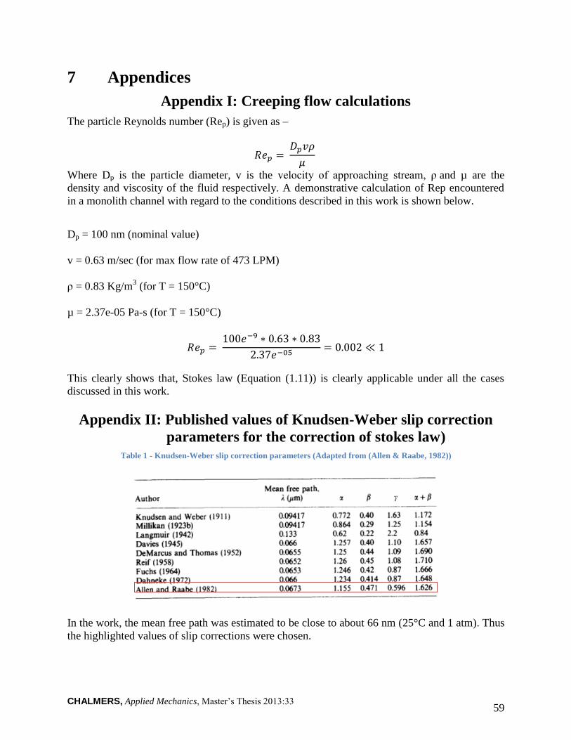
CHALMERS, Applied Mechanics, Master‘s Thesis 2013:33 59
7 Appendices
Appendix I: Creeping flow calculations
The particle Reynolds number (Rep) is given as –
Where Dp is the particle diameter, v is the velocity of approaching stream, ρ and µ are the
density and viscosity of the fluid respectively. A demonstrative calculation of Rep encountered
in a monolith channel with regard to the conditions described in this work is shown below.
Dp = 100 nm (nominal value)
v = 0.63 m/sec (for max flow rate of 473 LPM)
ρ = 0.83 Kg/m3 (for T = 150°C)
µ = 2.37e-05 Pa-s (for T = 150°C)
This clearly shows that, Stokes law (Equation (1.11)) is clearly applicable under all the cases
discussed in this work.
Appendix II: Published values of Knudsen-Weber slip correction
parameters for the correction of stokes law)
Table 1 - Knudsen-Weber slip correction parameters (Adapted from (Allen & Raabe, 1982))
In the work, the mean free path was estimated to be close to about 66 nm (25°C and 1 atm). Thus
the highlighted values of slip corrections were chosen.

CHALMERS, Applied Mechanics, Master‘s Thesis 2013:33 60
Appendix III: TOPAS ATM-230 operating pressure and
recirculation ratio
The following diagram displays the link between the ATM 230 operating pressure (bar) and the
produced aerosol flow rate (litre per minute) based on two different nozzle sizes (1.1 &1.3) as -
Figure 7.1a-The characteristic curve of the nozzles (1.1 &1.3)
More details regarding the expected particle size from the atomizer droplets (generated from
DEHS) are presented in following sections.
Figure 7.1b – PSD of DEHS (Di-Ethyl-Hexyl-Sebacat) measured by scanning mobility particle sizer
Di-Ethyl-Hexyl-Sebacat (DEHS) is a no soluble, colourless and odourless liquid which is
suitable for producing steady aerosols. The main proportion of droplets generated by aerosol
generators series ATM 230 can to be stated in the most penetration particle size (0.2...0.3µm).
The produced DEHS aerosol features very high particle concentrations (>107 particles/cm
3)
which is close to the aforementioned penetration particle size range.
The recirculation ratio of droplets in ATM 230 was also calculated as-

CHALMERS, Applied Mechanics, Master‘s Thesis 2013:33 61
First, a plate was placed under the baffle plate in order to block the passage of coarse droplet
stream from going back to the main solution container. In this way it was possible to calculate
Q1 which is the volumetric flow rate of escaped fine droplets. It took 25 seconds to use up 15 ml
salt solution. So, Q1 was calculated as: 15/25=0.65(ml/sec)
Then, the plate was removed and recirculation of coarse droplets into the system was allowed.
This took nearly 3 hours to use 25 ml of salt solution .Therefore, Q2 was calculated as:
25/10800=0.002 (ml/sec).By considering a simple mass balance, Q3 was calculated as: (Q1-Q2)
=0.65 (ml/sec) and finally the recirculation ratio was calculated as: Q3/Q2=300. This would
mean that, about 97% of the droplets formed are coarse, which would mean that they impact on
the baffle plate and fall back down into the main solution. The aerosol foam is formed by the
remaining 3% of the solution. This would in turn mean that, small volumes of solutions can
sustain for larger periods of time to provide the requisite PSD and number concentration desired.
A schematic flow sheet of this reaction is presented in the Figure below-
Figure 7.2 Recirculation ratio calculation of coarse particles produced at the TOPAS ATM-230 atomizer
Appendix IV: Preliminary trials
a) First sets of experiments
A D-optimal design with variable effects confounded is chosen. A D-optimal design is a
computer aided design which contains the best subset of all possible experiments. These designs
are straight optimizations based on a chosen optimality criterion. The design matrices are
usually not orthogonal and effect estimates are correlated. The statistical software MODDE was
used to generate the requisite D-optimal design. The design is as follows.
Table 7.3 Experimental design for preliminary trials (first set)
Exp No Pupstr(bar) Concentration(PPM) 1dil 2dil
1 3 10 1 -1
2 3 10 5 -1
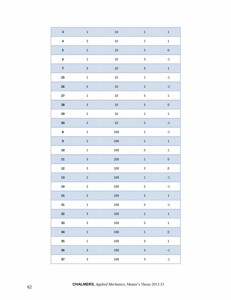
CHALMERS, Applied Mechanics, Master‘s Thesis 2013:33 62
3 1 10 1 1
4 3 10 1 1
5 1 10 5 0
6 1 10 3 -1
7 3 10 3 1
25 1 10 1 -1
26 3 10 1 -1
27 1 10 5 1
28 3 10 5 0
29 2 10 1 1
30 2 10 5 -1
8 1 100 1 -1
9 1 100 1 1
10 1 100 5 1
11 3 100 1 0
12 3 100 5 0
13 2 100 1 -1
14 2 100 5 -1
15 2 100 5 1
31 1 100 5 -1
32 3 100 1 1
33 3 100 5 1
34 1 100 1 0
35 1 100 3 1
36 3 100 3 -1
37 3 100 3 -1

CHALMERS, Applied Mechanics, Master‘s Thesis 2013:33 63
16 1 10000 1 -1
17 3 10000 1 -1
18 1 10000 5 -1
19 3 10000 5 -1
20 1 10000 1 1
21 3 10000 1 1
22 1 10000 5 1
23 3 10000 5 1
24 2 10000 3 0
38 1 10000 1 -1
39 3 10000 1 -1
40 1 10000 5 -1
41 3 10000 5 -1
42 1 10000 1 1
43 3 10000 1 1
44 1 10000 5 1
45 3 10000 5 1
46 2 10000 3 0
47 2 10000 3 0
48 2 10000 3 0
49 2 10000 3 0

CHALMERS, Applied Mechanics, Master‘s Thesis 2013:33 64
b) Second set of experiments
Table 7.4 Experimental design (33) for preliminary trials (second set)
Exp No. Concentration(PPM) Up stream pressure(bar)
Heated pipe (°C)
1 5000 1.5 40
2 5000 2.5 40
3 5000 3.5 40
4 10000 1.5 40
5 10000 2.5 40
6 10000 3.5 40
7 15000 1.5 40
8 15000 2.5 40
9 15000 3.5 40
10 5000 1.5 70
11 5000 2.5 70
12 5000 3.5 70
13 10000 1.5 70
14 10000 2.5 70
15 10000 3.5 70
16 10000 2.5 70
17 10000 2.5 70
18 10000 2.5 70
19 15000 1.5 70
20 15000 2.5 70
21 15000 3.5 70
22 5000 1.5 100
23 5000 2.5 100
24 5000 3.5 100
25 10000 1.5 100
26 10000 2.5 100
27 10000 3.5 100
28 15000 1.5 100
29 15000 2.5 100
30 15000 3.5 100

CHALMERS, Applied Mechanics, Master‘s Thesis 2013:33 65
Appendix V: EATS flow calculations (Reynolds number calculations
for EATS inlet and monolith channel)
a) Re at the EATS inlet
U = 2.56 m/sec
As the Re is lower than 2300 (laminar Re limit for pipes), the flow profile at the EATS inlet is
laminar.
b) Re in the channel
U = 0.63 m/sec
As the Re is significantly lower than 2300 (laminar Re limit for a square channel), the flow
profiles within the channels are clearly laminar
dc = 1.118mm U

CHALMERS, Applied Mechanics, Master‘s Thesis 2013:33 66
Appendix VI: Typical values of C2 (viscous resistance factor) along
with the corresponding monolith pressure drops
Table 7.5 – Inertial resistance factors used in the porous zone model
Pressure drop across the substrate
Inertial resistance factor(C2)
18.6 Pa 1.00E+07
28.47 Pa 8.00E+07
57.01 Pa 9.00E+07
The operating monolith pressures are obtained by manually adjusting this viscous resistance
factor. Typical values of C2 along with the corresponding monolith pressure drops are listed in
Table 7.5 above.
Appendix: VII UDF’s
Diffusivity
The following UDF calculates the ‗Brownian diffusion‘ co-efficient for particles of different
sizes diffusing together in air.
#include "udf.h" #include "dpm.h" #include "math.h" DEFINE_DIFFUSIVITY(Custom_diffusivity,c,t,i) { real Cc,Dab,Fd,cmol,mean_free_path; real Knp; real P_DIAM[27] ={4.87e-9,7.5e-9,10e-9,13.34e-9,15.4e-9,17.78e-9,20.54e-9,23.71e-9,27.38e-9,31.62e-9,36.52e-9,42.17e-9,48.7e-9,56.23e-9,64.94e-9,74.99e-9,86.6e-9,100e-9,115.48e-9,133.35e-9,159.99e-9,177.83e-9,205.35e-9,237.14e-9,273.84e-9,316.23e-9,365.17e-9}; /* Particle size bins */ if(i<27) { cmol = pow((8.0*101325.0/(M_PI*C_R(c,t))), 0.5); mean_free_path = C_MU_L(c,t)/(0.499*cmol*C_R(c,t)); Fd=3*M_PI*P_DIAM[i]*C_MU_L(c,t); /* Drag with Cunningham factor */ Knp = 2.0*mean_free_path/P_DIAM[i]; Cc = (1.0 + Knp*(1.257 + 0.406*exp(-1.1/Knp))); Dab = (1.3806488e-23)*C_T(c,t)*Cc/Fd; } else { Dab = 2.55e-5; /* species i is the gas */ } return Dab;
}

CHALMERS, Applied Mechanics, Master‘s Thesis 2013:33 67
Wall temperature profile
The following UDF sets a temperature profile on the walls of the channel. This temperature
profile is utilized primarily in the non-adiabatic simulations.
DEFINE_PROFILE(wall_ins_casea,thread,index) { real x[ND_ND]; /* this will hold the position vector */ real y,T; face_t f; begin_f_loop(f,thread) /* loops over all faces in the thread passed in the DEFINE macro argument */ { F_CENTROID(x,f,thread); y = x[2]; T = (82.4579*((pow(y,2.0))))+(45.7558*y)+(493.7469); F_PROFILE(f,thread,index) =T; } end_f_loop(f,thread)
}

CHALMERS, Applied Mechanics, Master‘s Thesis 2013:33 68
Appendix VIII: Mesh quality study
a) EATS
As elucidated in the earlier sections, the quality of the chosen mesh would have a significant
impact on the nature of the results that can be obtained from a particular simulation. The effect of
the mesh quality has been studied by solving the velocity field for four different meshes, each
with successively larger number of computational cells. The velocity of the outlet is plotted as a
function of the number of cells. The results of this study are as follows
Figure 7.3 – Solution mesh independency study
The solutions (mass weighted average of outlet velocity) from 5 different meshes are compared
in the Figure 7.3 above .The figure above confirms the fact that the solution to the EATS flow
field becomes mesh independent when the minimum number of cells in the mesh exceeds about
100000 cells. Hence the mesh chosen for all the further computations had a size of about 115000
cells. The quality of the chosen mesh is also very apparent in the contour plot below.
Figure 7.4 - Contours coloured by velocity magnitude coarse mesh (left) and fine mesh (right)
Clearly the finer mesh is able to resolve the flow in the recirculation zones (diverging section of
the geometry) much better than the coarser one.

CHALMERS, Applied Mechanics, Master‘s Thesis 2013:33 69
b) Channel
The quality of the mesh employ to simulate the single channel was assessed. This study is very
critical in order to ensure that the solution can be trusted (well resolved) and at the same time is
mesh independent. The effect of the mesh quality has been studied by solving the velocity field
for four different meshes, each with successively larger number of computational cells. The
velocity of the outlet is plotted as a function of the number of cells. The results of this study are
as follows
Figure 7.5 – Mesh independency studies
The solutions (mass weighted average of outlet velocity) from 5 different meshes are compared
in the Figure 7.5 above .The figure above confirms the fact that the solution to the EATS flow
field becomes mesh independent when the minimum number of cells in the mesh exceeds about
400000 cells. Hence the mesh chosen for all the further computations had a size of about 927000
cells. The quality of the chosen mesh is also very apparent in the contour plot below (velocity is
well resolved in the finer mesh).

CHALMERS, Applied Mechanics, Master‘s Thesis 2013:33 70
Figure 7.6 - Contours coloured by velocity magnitude coarse mesh (top left) , fine mesh with wall refine ( top right),
coarse mesh (bottom left) and wall-refined mesh (bottom right)

CHALMERS, Applied Mechanics, Master‘s Thesis 2013:33 71
Appendix IX: Temperature profile comparison between
experiments and simulations
As mentioned earlier, some preliminary studies were done in the EATS with just air (no
particulate flow). These studies were done in order to establish whether the conditions predicted
by the simulations were actually encountered in reality. A comparison between the temperature
field measured in real time using the thermocouples (described above) and the field predicted by
the CFD data would thus be a very good way to validate the simulations. The simulations done
at a flow rate of 150 LPM and 250°C with insulation were chosen. The temperature profile
corresponding to thermocouple positions 3, 5 and 8 were chosen from the EATS simulation.
These were then compared with the data recorded by thermocouples 3, 5 and 8 during the
experiment trials under the same conditions. This comparison is plotted in the Figure (7.7)
below.
Figure 7.7 - Comparison between CFD data and measure values
The simulations predicted a temperature drop of about 10 K (see Figure above). The values
measured by the thermocouple (averaged over time) indicated a temperature drop (along the
same position) of about 12 K. This indicates that the simulation indeed correspond well with the
experiments. This trend is noted even when comparing other EATS operating points with
experimental measurement of temperature.
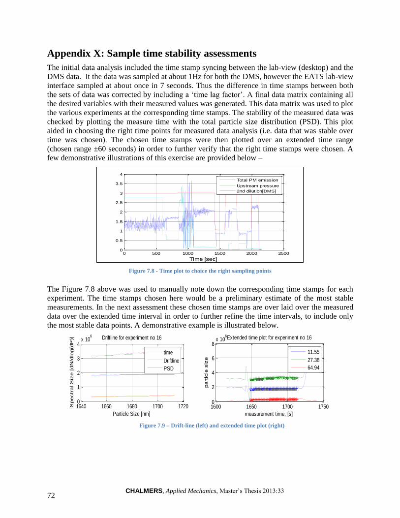
CHALMERS, Applied Mechanics, Master‘s Thesis 2013:33 72
Appendix X: Sample time stability assessments
The initial data analysis included the time stamp syncing between the lab-view (desktop) and the
DMS data. It the data was sampled at about 1Hz for both the DMS, however the EATS lab-view
interface sampled at about once in 7 seconds. Thus the difference in time stamps between both
the sets of data was corrected by including a ‗time lag factor‘. A final data matrix containing all
the desired variables with their measured values was generated. This data matrix was used to plot
the various experiments at the corresponding time stamps. The stability of the measured data was
checked by plotting the measure time with the total particle size distribution (PSD). This plot
aided in choosing the right time points for measured data analysis (i.e. data that was stable over
time was chosen). The chosen time stamps were then plotted over an extended time range
(chosen range ±60 seconds) in order to further verify that the right time stamps were chosen. A
few demonstrative illustrations of this exercise are provided below –
Figure 7.8 - Time plot to choice the right sampling points
The Figure 7.8 above was used to manually note down the corresponding time stamps for each
experiment. The time stamps chosen here would be a preliminary estimate of the most stable
measurements. In the next assessment these chosen time stamps are over laid over the measured
data over the extended time interval in order to further refine the time intervals, to include only
the most stable data points. A demonstrative example is illustrated below.
Figure 7.9 – Drift-line (left) and extended time plot (right)
0 500 1000 1500 2000 25000
0.5
1
1.5
2
2.5
3
3.5
4
Time [sec]
Total PM emission
Upstream pressure
2nd dilution[DMS]
1640 1660 1680 1700 17200
1
2
3
4x 10
6
Particle Size [nm]
Spectr
al S
ize [
dN
/dlo
g(d
P)] Driftline for experiment no 16
time
Driftline
PSD
1600 1650 1700 17500
2
4
6
8x 10
6
measurement time, [s]
part
icle
siz
e
Extended time plot for experiment no 16
11.55
27.38
64.94

CHALMERS, Applied Mechanics, Master‘s Thesis 2013:33 73
Appendix XI: CE Experiments
Table 7.6 - Non-adiabatic CE trials operating conditions
Exp No.
Average
Temperature
(deg C)
Pressure
across
substrate
(Pa)
Flow
rate
(LPM) Sampling
positions
Concent-
ration
Up
stream
pressure
Heated pipe
temperature
(°C)
Total
dilution
at DMS
DMS
Sample
flow
(LPM)
Number
concentration
at 28 nm peak
(N/cc)
Total number
concentration
measured at
DMS (N/cc)
Preliminary
CE
measured at
28 nm (%)
1
18.6 150
Bef 10000 4 bar 200 10 8.1 395000 303500 24.05
After 10000 4 bar 200 10 8.11
300000 245000
2 Bef 10000 4 bar 200 10 8.05
380000 298150 21.05
After 10000 4 bar 200 10 8.07
300000 245000
3
Bef 10000 4 bar 200 10 8.03
385000 298350 23.37
After 10000 4 bar 200 10 8.09
295000 240000
4
130.5 28.47 236
Bef 10000 4 bar 200 10 8.07 230000 171000 17.39
After 10000 4 bar 200 10 8.11
190000 153500
5 Bef 10000 4 bar 200 10 8.02
231000 171000 17.74
After 10000 4 bar 200 10 8.07
190000 152000
6
Bef 10000 4 bar 200 10 8.03
230000 179000 17.39
After 10000 4 bar 200 10 8.09
190000 152000
7
57.01 473
Bef 10000 4 bar 200 10 8.06 120000 95000 12.5
After 10000 4 bar 200 10 8.09
105000 85600
8 Bef 10000 4 bar 200 10 8.05
125000 96800 12
After 10000 4 bar 200 10 8.09
110000 83750

CHALMERS, Applied Mechanics, Master‘s Thesis 2013:33 74
9 Bef
10000 4 bar 200 10 8.05 125000 94000 14
After 10000 4 bar 200 10 8.05
107500 85600
10
18.8 150
Bef 10000 4 bar 200 11.98 8.08
980000 800000 28.57
After 10000 4 bar 200 12 8.08
700000 615000
11 Bef 10000 4 bar 200 11.99 7.99
980000 800000 26.53
After 10000 4 bar 200 12.03 8.08
720000 612000
12
Bef 10000 4 bar 200 11.98 8.03
1000000 800000 28
After 10000 4 bar 200 12 8
720000 610000
13
172.5 28.59 236
Bef 10000 4 bar 200 11.75 8.04
680000 515000 17.64
After 10000 4 bar 200 12 8.07
560000 415000
14 Bef 10000 4 bar 200 11.94 8.05
680000 525000 20.58
After 10000 4 bar 200 12.03 8.02
540000 420000
15
Bef 10000 4 bar 200 12.05 8.03
675000 530000 20.75
After 10000 4 bar 200 12 8.039
540000 420000
16
57.15 473
Bef 10000 4 bar 200 12.04 8.08
380000 295000 14.47
After 10000 4 bar 200 12 8.08
325000 255000
17 Bef 10000 4 bar 200 12.03 8.05
380000 300000 15.78
After 10000 4 bar 200 12 8.09
320000 260000
18
Bef 10000 4 bar 200 12.05 8.05
381000 300000 10.76
After 10000 4 bar 200 12 8.05
340000 262500
19
18.8 150
Bef 10000 4 bar 200 15 7.98
900000 786565 26.67

CHALMERS, Applied Mechanics, Master‘s Thesis 2013:33 75
After 10000 4 bar 200 15 8.01
660000 600500
20 Bef 10000 4 bar 200 15 8.02
920000 790000 28.26
After 10000 4 bar 200 15 8.04
660000 600500
21
Bef 10000 4 bar 200 15 8.03
920000 775000 28.26
After 10000 4 bar 200 15 8.05
660000 600000
22
213.5 31.65 236
Bef 10000 4 bar 200 15 8.04
680000 580000 26.47
After 10000 4 bar 200 15 8.05
500000 470000
23 Bef 10000 4 bar 200 15 8.05
660000 550000 24.24
After 10000 4 bar 200 15 8.02
500000 445000
24
Bef 10000 4 bar 200 15 8.03
660000 550000 18.18
After 10000 4 bar 200 15 8.039
500000 450000
25
63.56 473
Bef 10000 4 bar 200 15 8.06
375000 306000 17.33
After 10000 4 bar 200 15 8.09
310000 270000
26 Bef 10000 4 bar 200 15 8.05
360000 315000 16.67
After 10000 4 bar 200 15 8.09
300000 278750
27
Bef 10000 4 bar 200 15 8.05
360000 310000 16.67
After 10000 4 bar 200 15 8.05
300000 275000

CHALMERS, Applied Mechanics, Master‘s Thesis 2013:33 76
Table 7.7 - Adiabatic CE trials operating conditions
Exp No.
Average
Temperature
(deg C)
Pressure
across
substrate
(Pa)
Flow
rate
(LPM) State
Concent-
ration
Up
stream
pressure
Heated pipe
temperature
(°C)
Total
dilution
at DMS
DMS
Sample
flow
(LPM)
Number
concentration
at 28 nm peak
(N/cc)
Total number
concentration
measured at
DMS (N/cc)
Preliminary CE
measured at 28
nm (%)
28
18.6 150
Bef 10000 4 bar 200 11.98 8.05 680000 520000 26.47
After 10000 4 bar 200 12 8.11 500000 410000
29 Bef 10000 4 bar 200 12.03 8.05 675000 510000 25.78
After 10000 4 bar 200 12.03 8.07 501000 410000
30 Bef 10000 4 bar 200 12.05 8.03 670000 495000 25.37
After 10000 4 bar 200 12 8.09 500000 405000
31
152.3 28.47 236
Bef 10000 4 bar 200 11.98 8.07 400000 310000 18.75
After 10000 4 bar 200 12 8.11 325000 260000
32 Bef 10000 4 bar 200 11.99 8.02 400000 300000 18.75
After 10000 4 bar 200 12.03 8.07 325000 265000
33 Bef 10000 4 bar 200 12.05 8.03 400000 305000 18.03
After 10000 4 bar 200 12 8.09 320000 250000
34
57.01 473
Bef 10000 4 bar 200 11.98 8.06 155000 115000 16.13
After 10000 4 bar 200 12 8.09 130000 100000
35 Bef 10000 4 bar 200 12.03 8.05 150000 115000 13.33
After 10000 4 bar 200 12 8.09 130000 98000
36 Bef 10000 4 bar 200 12.05 8.05 145000 106000 13.79

CHALMERS, Applied Mechanics, Master‘s Thesis 2013:33 77
After 10000 4 bar 200 12 8.05 125000 97000
37
18.8 150
Bef 10000 4 bar 200 11.98 8.06 225000 185000 37.78
After 10000 4 bar 200 12 8.01 140000 115000
38 Bef 10000 4 bar 200 11.99 7.99 220000 180000 36.37
After 10000 4 bar 200 12.03 8.07 140000 115000
39 Bef 10000 4 bar 200 11.98 8.03 210000 179000 38.1
After 10000 4 bar 200 12 8 130000 110000
40
201.7 28.59 236
Bef 10000 4 bar 200 11.75 8.04 140000 100000 28.57
After 10000 4 bar 200 12 8.07 100000 70100
41 Bef 10000 4 bar 200 11.94 8.05 139500 100500 29.89
After 10000 4 bar 200 12.03 8.02 97800 68500
42 Bef 10000 4 bar 200 12.05 8.03 137500 100000 30.5
After 10000 4 bar 200 12 8.039 94800 69500
43
57.15 473
Bef 10000 4 bar 200 12.04 8.06 61500 41000 18.69
After 10000 4 bar 200 12 8.09 50000 30000
44 Bef 10000 4 bar 200 12.03 8.05 62000 42100 19.35
After 10000 4 bar 200 12 8.09 50000 31075
45 Bef 10000 4 bar 200 12.05 8.05 65000 42500 19.07
After 10000 4 bar 200 12 8.05 52600 31700
46
18.8 150 Bef 10000 4 bar 200 12 7.98 170000 146500 41.17

CHALMERS, Applied Mechanics, Master‘s Thesis 2013:33 78
After 10000 4 bar 200 12 8.01 100000 90000
47 Bef 10000 4 bar 200 11.99 8.02 168000 140000 40.47
After 10000 4 bar 200 12.03 8.04 100000 88000
48 Bef 10000 4 bar 200 11.98 8.03 170000 139000 41.17
After 10000 4 bar 200 12 8.05 100000 90000
49
252.35 31.65 236
Bef 10000 4 bar 200 11.75 8.04 100000 88070 25
After 10000 4 bar 200 11.99 8.05 75000 59000
50 Bef 10000 4 bar 200 11.94 8.05 100000 88006.5 30
After 10000 4 bar 200 12.03 8.02 70000 60000
51 Bef 10000 4 bar 200 12.05 8.03 100000 80000 27.63
After 10000 4 bar 200 12 8.039 70000 57895
52
63.56 473
Bef 10000 4 bar 200 12.04 8.06 50000 40600 20
After 10000 4 bar 200 12 8.09 40000 30000
53 Bef 10000 4 bar 200 12.03 8.05 52500 38000 26.67
After 10000 4 bar 200 12 8.09 38500 28750
54 Bef 10000 4 bar 200 12.05 8.05 51500 38500 22.33
After 10000 4 bar 200 12 8.05 40000 29000

CHALMERS, Applied Mechanics, Master‘s Thesis 2013:33 79
Appendix XII: Non-adiabatic set up (Case II)
Effect of residence time on CE (at 150°C )
The effect of residence time for experiment numbers 2, 7 and 15 is evaluated (non-adiabatic set-
up) .Also, the PSDbefore and PSDafter results which are representing calculation of each single
capture efficiency curve are also presented for each case. The results are presented in the Figure
(7.11) below-
Figure 7.10 - Effect of residence time on capture efficiency at 150°C, non- adiabatic set up
Effect of residence time on CE (at 200°C )
The effect of residence time for experiment numbers 11, 14 and 17 is evaluated (non-adiabatic
set-up and 200°C). The PSDbefore and PSDafter results which are representing calculation of each
single capture efficiency curve are also presented for each case. The flow conditions for different
cases are listed in the Table (7.8).
101
102
0
20
40
60
80
100
Particle Size [nm]
Ca
ptu
re e
ffic
ien
cy [%
]
150LPM[150 Deg C,no:2]
236LPM[150 Deg C,no:7]
473LPM[150 Deg C,no:15]
101
102
0
1
2
3x 10
5
Particle Size [nm]P
art
icle
num
ber
[dN
/dlo
g(d
P)]
psdbef ore,150 deg c,150LPM,no:2
psdaf ter,150 deg c,150LPM,no:2
101
102
0
2
4
6
x 105
Particle Size [nm]
Part
icle
num
ber
[dN
/dlo
g(d
P)]
psdbef ore,150 deg c,473LPM,no:7
psdaf ter,150 deg c,473PM,no:7
101
102
0
1
2
3
4
5x 10
5
Particle Size [nm]
Part
icle
num
ber
[dN
/dlo
g(d
P)]
psdbef ore,150 deg c,473LPM,no:15
psdaf ter,150 deg c,473PM,no:15
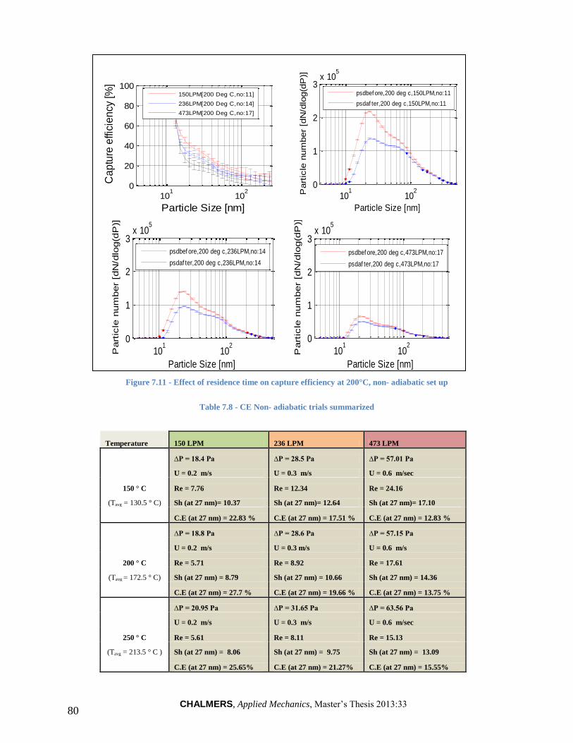
CHALMERS, Applied Mechanics, Master‘s Thesis 2013:33 80
Figure 7.11 - Effect of residence time on capture efficiency at 200°C, non- adiabatic set up
Table 7.8 - CE Non- adiabatic trials summarized
101
102
0
20
40
60
80
100
Particle Size [nm]
Ca
ptu
re e
fficie
ncy [%
]
150LPM[200 Deg C,no:11]
236LPM[200 Deg C,no:14]
473LPM[200 Deg C,no:17]
101
102
0
1
2
3x 10
5
Particle Size [nm]
Part
icle
num
ber
[dN
/dlo
g(d
P)]
psdbef ore,200 deg c,150LPM,no:11
psdaf ter,200 deg c,150LPM,no:11
101
102
0
1
2
3x 10
5
Particle Size [nm]
Part
icle
num
ber
[dN
/dlo
g(d
P)]
psdbef ore,200 deg c,236LPM,no:14
psdaf ter,200 deg c,236LPM,no:14
101
102
0
1
2
3x 10
5
Particle Size [nm]
Part
icle
num
ber
[dN
/dlo
g(d
P)]
psdbef ore,200 deg c,473LPM,no:17
psdaf ter,200 deg c,473LPM,no:17
Temperature 150 LPM 236 LPM 473 LPM
∆P = 18.4 Pa ∆P = 28.5 Pa ∆P = 57.01 Pa
U = 0.2 m/s U = 0.3 m/s U = 0.6 m/sec
150 ° C Re = 7.76 Re = 12.34 Re = 24.16
(Tavg = 130.5 ° C) Sh (at 27 nm)= 10.37 Sh (at 27 nm)= 12.64 Sh (at 27 nm)= 17.10
C.E (at 27 nm) = 22.83 % C.E (at 27 nm) = 17.51 % C.E (at 27 nm) = 12.83 %
∆P = 18.8 Pa ∆P = 28.6 Pa ∆P = 57.15 Pa
U = 0.2 m/s U = 0.3 m/s U = 0.6 m/s
200 ° C Re = 5.71 Re = 8.92 Re = 17.61
(Tavg = 172.5 ° C) Sh (at 27 nm) = 8.79 Sh (at 27 nm) = 10.66 Sh (at 27 nm) = 14.36
C.E (at 27 nm) = 27.7 % C.E (at 27 nm) = 19.66 % C.E (at 27 nm) = 13.75 %
∆P = 20.95 Pa ∆P = 31.65 Pa ∆P = 63.56 Pa
U = 0.2 m/s U = 0.3 m/s U = 0.6 m/sec
250 ° C Re = 5.61 Re = 8.11 Re = 15.13
(Tavg = 213.5 ° C ) Sh (at 27 nm) = 8.06 Sh (at 27 nm) = 9.75 Sh (at 27 nm) = 13.09
C.E (at 27 nm) = 25.65% C.E (at 27 nm) = 21.27% C.E (at 27 nm) = 15.55%

CHALMERS, Applied Mechanics, Master‘s Thesis 2013:33 81
Appendix XIII: Adiabatic set up (Case I)
Effect of residence time on CE (at 150 and 200 °C)
The effect of residence time for two remaining flow temperature of 150 (Figure 4.13) and 200°C
(Figure 4.14) were assessed and are separately evaluated in this section. In addition, the PSDbefore
and PSDafter results which are representing calculation of each single capture efficiency curve are
also presented for each case.
Figure 7.12- Effect of residence time on capture efficiency at 150 °C, Adiabatic set up [ exp no: 29,32 and35]
101
102
0
20
40
60
80
100
Particle Size [nm]
Ca
ptu
re e
ffic
ien
cy [%
]
150 LPM C[150 Deg C,exp no:29]
236 LPM C[150 Deg C,exp no:32]
473 LPM C[150 Deg C,exp no:35]
101
102
0
2
4
6x 10
5
Particle Size [nm]
Part
icle
num
ber
[dN
/dlo
g(d
P)]
psdbef ore,150 deg c,150LPM,no:29
psdaf ter,150 deg c,150PM,no:29
101
102
0
2
4
x 105
Particle Size [nm]Part
icle
num
ber
[dN
/dlo
g(d
P)]
psdbef ore,150 deg c,236LPM,no:32
psdaf ter,150 deg c,236PM,no:32
101
102
0
2
4
x 105
Particle Size [nm]Part
icle
num
ber
[dN
/dlo
g(d
P)]
psdbef ore,150 deg c,473LPM,no:35
psdaf ter,150 deg c,473PM,no:35
101
102
0
20
40
60
80
100
Particle Size [nm]
Ca
ptu
re e
ffic
ien
cy [%
]
150 LPM C[200 Deg C,exp no:37]
236 LPM C[200 Deg C,exp no:40]
473 LPM C[200 Deg C,exp no:44]
101
102
0
5
10
x 105
Particle Size [nm]
Part
icle
num
ber
[dN
/dlo
g(d
P)]
psdbef ore,200 deg c,150LPM,no:37
psdaf ter,200 deg c,150LPM,no:37
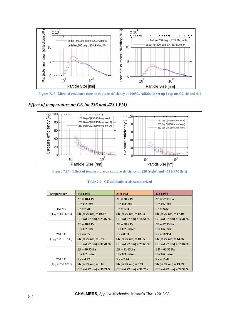
CHALMERS, Applied Mechanics, Master‘s Thesis 2013:33 82
Figure 7.13- Effect of residence time on capture efficiency at 200°C, Adiabatic set up [ exp no :37, 40 and 44]
Effect of temperature on CE (at 236 and 473 LPM)
Figure 7.14 - Effect of temperature on capture efficiency at 236 (right) and 473 LPM (left)
Table 7.9 - CE adiabatic trials summarized
Temperature 150 LPM 236LPM 473 LPM
∆P = 18.4 Pa ∆P = 28.5 Pa ∆P = 57.01 Pa
U = 0.2 m/s U = 0.3 m/s U = 0.6 m/s
150 °C Re = 7.78 Re = 12.33 Re = 24.65
(Tavg = 149.6 °C) Sh (at 27 nm) = 10.37 Sh (at 27 nm) = 12.63 Sh (at 27 nm) = 17.10
C.E (at 27 nm) = 25.87 % C.E (at 27 nm) = 18.51 % C.E (at 27 nm) = 14.41 %
∆P = 18.8 Pa ∆P = 28.6 Pa ∆P = 57.15 Pa
U = 0.2 m/s U = 0.2 m/sec U = 0.6 m/s
200 ° C Re = 6.05 Re = 8.83 Re = 16.954
(Tavg = 201.6 ° C) Sh (at 27 nm) = 8.79 Sh (at 27 nm) = 10.65 Sh (at 27 nm) = 14.36
C.E (at 27 nm) = 37.41 % C.E (at 27 nm) = 29.65 % C.E (at 27 nm) = 19.04 %
∆P = 20.95 Pa ∆P = 31.65 Pa ∆ P = 63.56 Pa
U = 0.2 m/sec U = 0.3 m/sec U = 0.6 m/sec
250 ° C Re = 4.47 Re = 7.74 Re = 15.49
(Tavg = 252.6 °C) Sh (at 27 nm) = 8.06 Sh (at 27 nm) = 9.74 Sh (at 27 nm) = 13.09
C.E (at 27 nm) = 39.21% C.E (at 27 nm) = 31.2% C.E (at 27 nm) = 22.99%
101
102
0
5
10
x 105
Particle Size [nm]
Part
icle
num
ber
[dN
/dlo
g(d
P)]
psdbef ore,200 deg c,236LPM,no:40
psdaf ter,200 deg c,236LPM,no:40
101
102
0
5
10
x 105
Particle Size [nm]
Part
icle
num
ber
[dN
/dlo
g(d
P)]
psdbef ore,200 deg c,473LPM,no:44
psdaf ter,200 deg c,473LPM,no:44
101
102
0
20
40
60
80
100
Particle Size [nm]
Ca
ptu
re e
ffic
ien
cy [%
]
150 Deg C[236LPM,exp no:4]
200 Deg C[236LPM,exp no:11]
250 Deg C[236LPM,exp no:14]
101
102
0
20
40
60
80
100
Particle Size [nm]
Ca
ptu
re e
ffic
ien
cy [%
]
150 Deg C[473LPM,exp no:36]
200 Deg C[473LPM,exp no:44]
250 Deg C[473LPM,exp no:54]

CHALMERS, Applied Mechanics, Master‘s Thesis 2013:33 83
Appendix XIV
Comparison between adiabatic & non-adiabatic at different flow conditions are presented in the
Figure (7.15) below-
Figure 7.15- The comparison between two set ups, Adiabatic and non-adiabatic
101
102
0
20
40
60
80
100
Particle Size [nm]
Ca
ptu
re e
ffic
ien
cy [%
]
Adiab,250 deg C[473 LPM,no:52]
Non-adiab,250 deg C[473 LPM,no:27]
101
102
0
20
40
60
80
100
Particle Size [nm]
Ca
ptu
re e
ffic
ien
cy [%
]
Adiab,150 deg C[150 LPM,no:29]
Non-adiab,150 deg C[150LPM,no:2]
101
102
0
20
40
60
80
100
Particle Size [nm]
Ca
ptu
re e
ffic
ien
cy [%
]
Adiab,150 deg C[236 LPM,no:33]
Non-adiab,150 deg C[236 LPM,no:6]

CHALMERS, Applied Mechanics, Master‘s Thesis 2013:33 84
Appendix XV: Temperature profile comparison from simulations
Figure 7.16 –Temperature profile for non-adiabatic substrate at 150°C and 473 LPM. The black, green and red lines
represent temperature gradients at the beginning, middle and end of substrate respectively.
Figure 7.17 – Temperature profile for non-adiabatic substrate at 250°C and 150 LPM. The black green and red lines
represent temperature gradients at the beginning, middle and end of substrate respectively.
The Figure 7.16 above represents the lower residence time (473 LPM) and lower temperature
(150 °C). It is very apparent that the radial gradient is almost zero at a distance of quarter
distance from the centre. The Figure 7.17 represents higher residence time (150 LPM) and higher
temperature (250 °C) and it is easy to notice that temperature gradient starts from the centre of
the geometry. Therefore, it can be concluded that in the first case, the average temperature of
channels is higher than the second case.

CHALMERS, Applied Mechanics, Master‘s Thesis 2013:33 85
Appendix XVI: Comparison between experiments and simulations
a) Adiabatic conditions
Comparison at constant temperatures
Figure 7.18 – Comparison between experiments and simulations at 200°C
Figure 7.19 - Comparison between experiments and simulations at 250°C
101
102
0
10
20
30
40
50
60
70
80
90
100
Particle Size [nm]
Ca
ptu
re E
ffici
en
cy ±
err
or
(t*s
qrt
(va
r(X
*1/Y
)) [%
]
CE experimental at Q = 150 LPM
CE theoretical at Q = 150 LPM
CE experimental at Q = 236 LPM
CE theoretical at Q = 236 LPM
CE experimental at Q = 473 LPM
CE theoretical at Q = 473 LPM
101
102
0
10
20
30
40
50
60
70
80
90
100
Particle Size [nm]
Ca
ptu
re E
ffic
ien
cy ±
err
or
(t*s
qrt
(va
r(X
*1/Y
)) [%
]
CE experimental at Q = 150 LPM
CE theoretical at Q = 150 LPM
CE experimental at Q = 236 LPM
CE theoretical at Q = 236 LPM
CE experimental at Q = 473 LPM
CE theoretical at Q = 473 LPM
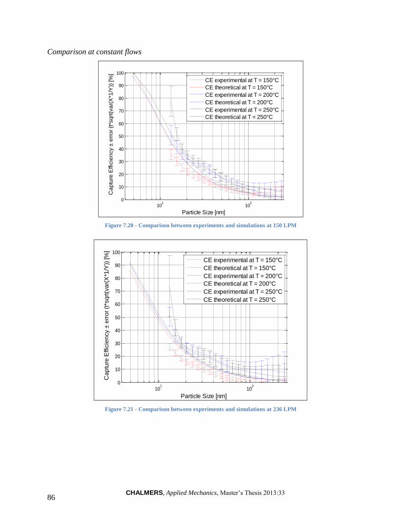
CHALMERS, Applied Mechanics, Master‘s Thesis 2013:33 86
Comparison at constant flows
Figure 7.20 - Comparison between experiments and simulations at 150 LPM
Figure 7.21 - Comparison between experiments and simulations at 236 LPM
101
102
0
10
20
30
40
50
60
70
80
90
100
Particle Size [nm]
Ca
ptu
re E
ffic
ien
cy ±
err
or
(t*s
qrt
(va
r(X
*1/Y
)) [%
]
CE experimental at T = 150°C
CE theoretical at T = 150°C
CE experimental at T = 200°C
CE theoretical at T = 200°C
CE experimental at T = 250°C
CE theoretical at T = 250°C
101
102
0
10
20
30
40
50
60
70
80
90
100
Particle Size [nm]
Ca
ptu
re E
ffic
ien
cy ±
err
or
(t*s
qrt
(va
r(X
*1/Y
)) [%
]
CE experimental at T = 150°C
CE theoretical at T = 150°C
CE experimental at T = 200°C
CE theoretical at T = 200°C
CE experimental at T = 250°C
CE theoretical at T = 250°C

CHALMERS, Applied Mechanics, Master‘s Thesis 2013:33 87
b) Non adiabatic conditions
Figure 7.22 - Comparison of CE obtained from experiments and simulations (channel close the walls) at 250°C, 150 LPM
Figure 7.23 - Comparison of CE obtained from experiments and simulations (channel quarter distance away from the
walls) at 250°C, 150 LPM
Figures 7.18 through 7.23 demonstrate that there is a good congruence between experiments and
simulations at all chosen EATS operation points.
101
102
0
10
20
30
40
50
60
70
80
90
100
Particle Size [nm]
Ca
ptu
re E
ffic
ien
cy ±
err
or
[%]
CE from experiments
CE from simulations
101
102
0
10
20
30
40
50
60
70
80
90
100
Particle Size [nm]
Ca
ptu
re E
ffic
ien
cy ±
err
or
[%]
CE from experiments
CE from simulations

CHALMERS, Applied Mechanics, Master‘s Thesis 2013:33 88
Appendix XVII: Sensitivity Analysis
Effect of monolith choice (channel hydraulic diameter) on CE
Square cell geometry in the wall-flow monolith with its characteristic checkerboard cell plugging
pattern is shown in Figure 7.24. A number of monolith properties can be expressed in terms of
the wall thickness (w) and the cell repeat distance (s), also known as the cell spacing (Gulati,
Cybulski, & Moulijn, 1998)
Figure 7.24 - Cell Geometry
The substrate cell density (N), defined as the number of channels per unit of cross-sectional area,
is given for square cell geometry by Equation (1). The metric unit of cell density is 1/cm2, with
the customary unit of cells per square inch (cpsi) widely used in the industry.
N = 1/s2
(1.1)
Cell hydraulic diameter (dh) is a measure of channel size used in hydraulics, mass transfer and
heat transfer calculations. In the case of square cells, it can be simply expressed as the difference
between repeat distance and wall thickness, as follows:
dh = s – w (1.2)
The commercial cell substrates along with the respective values for ‘s’ and ‘w’ are provided in
the table below –
Table 7.10 – Common substrate geometries used in diesel cars
Geometry4
type
Repeat distance (s) in
mm
Wall Thickness (w)
in mm
Hydraulic diameter (dh)
in mm
300/6 1.46 0.15 1.31
400/6 1.27 0.15 1.11
500/6 1.13 0.15 0.98
600/6 1.03 0.15 0.88
The CE sensitivity (plotted using the theoretical CE expression Equation (1.15)) towards the
change in geometry is shown in the figure below –
4 The geometry provides 300, 400, 500 and 600 cell substrates per square inch (cpsi) with a wall of thickness
6/1000th of an inch.

CHALMERS, Applied Mechanics, Master‘s Thesis 2013:33 89
Figure 7.25 – Sensitivity of CE towards monolith type (varying dh) at 250°C and 150 LPM
The 600/6 monolith has the highest CE due to the smaller hydraulic diameter (shorter diffusion
lengths). The noticeable trend is increase in CE with increase in cpsi of the monolith.
Effect of temperature on CE
The effect of temperature on CE has been extensively demonstrated in the Section 4.0. This
appendix would extend this discussion by reaching the upper boundaries of conventional engine
exhaust. Temperatures of 150, 250, 350 and 450°C have been examined (plotted using the
theoretical CE expression Equation (1.15)).
Figure 7.26 - Sensitivity of CE towards temperature at 150 LPM
Effect of engine exhaust flow on CE
Maximum exhaust gas flow is an important parameter for the aftertreatment device and other
exhaust system components. Exhaust flow data may be available from the engine manufacturer
or from other sources. Comprehensive listings of maximum exhaust gas flow and temperature
100
101
102
103
0
20
40
60
80
100
Particle Size [nm]
Captu
re e
ffic
iency [%
]
300/6 monolith
400/6 monolith
500/6 monolith
600/6 monolith
100
101
102
103
0
20
40
60
80
100
Particle Size [nm]
Captu
re e
ffic
iency [%
]
T = 150°C
T = 250°C
T = 350°C
T = 450°C
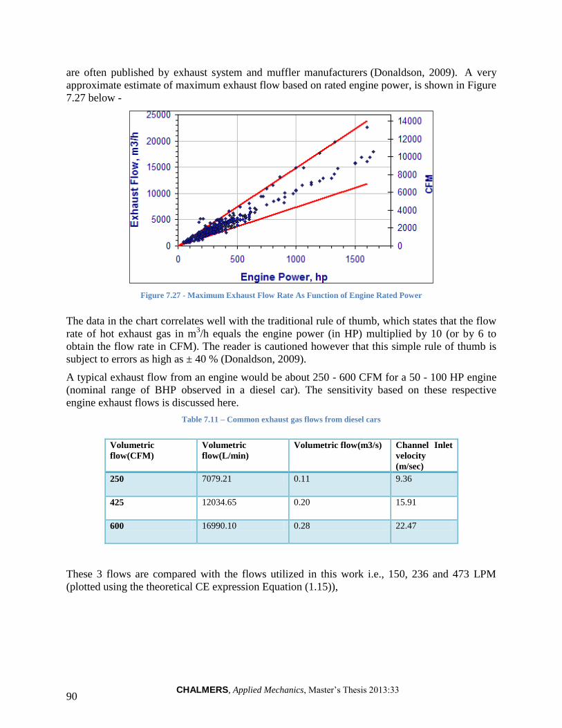
CHALMERS, Applied Mechanics, Master‘s Thesis 2013:33 90
are often published by exhaust system and muffler manufacturers (Donaldson, 2009). A very
approximate estimate of maximum exhaust flow based on rated engine power, is shown in Figure
7.27 below -
Figure 7.27 - Maximum Exhaust Flow Rate As Function of Engine Rated Power
The data in the chart correlates well with the traditional rule of thumb, which states that the flow
rate of hot exhaust gas in m3/h equals the engine power (in HP) multiplied by 10 (or by 6 to
obtain the flow rate in CFM). The reader is cautioned however that this simple rule of thumb is
subject to errors as high as ± 40 % (Donaldson, 2009).
A typical exhaust flow from an engine would be about 250 - 600 CFM for a 50 - 100 HP engine
(nominal range of BHP observed in a diesel car). The sensitivity based on these respective
engine exhaust flows is discussed here.
Table 7.11 – Common exhaust gas flows from diesel cars
Volumetric
flow(CFM)
Volumetric
flow(L/min)
Volumetric flow(m3/s) Channel Inlet
velocity
(m/sec)
250 7079.21 0.11 9.36
425 12034.65 0.20 15.91
600 16990.10 0.28 22.47
These 3 flows are compared with the flows utilized in this work i.e., 150, 236 and 473 LPM
(plotted using the theoretical CE expression Equation (1.15)),

CHALMERS, Applied Mechanics, Master‘s Thesis 2013:33 91
Figure 7.28 - Sensitivity of CE towards engine exhaust flow at 250°C
The common exhaust flows (7080, 12035 and 16990 LPM) noticed in a conventional diesel
automotive would correspond to significantly lower ranges for PM CE (about 1- 20 % for a
particle size range between 5- 90 nm). If these flows were chosen as experimental operating
conditions, it would be very hard to notice any significant trends in the CE. Moreover at such
high flows, the DMS signal to noise ratio would also be high leading to PM measurement at
levels very close to the limit of detection of the instrument. Thus in order to appreciate the
varying trends noticeable in CE of PM in an open substrate it is necessary that the substrate
flows are sufficiently low.
100
101
102
103
0
20
40
60
80
100
Particle Size [nm]
Captu
re e
ffic
iency [%
]
Q = 150 LPM
Q = 473 LPM
Q = 7080 LPM
Q = 12035 LPM
Q = 16990 LPM

CHALMERS, Applied Mechanics, Master‘s Thesis 2013:33 92
Appendix XVIII: Accuracy of CFD results
Figure 7.29 - Scaled residuals (for adiabatic channel simulation at 250°C and 150 LPM)
The Figure 7.29 above clearly demonstrates that the residuals of the solved variables (like x-
velocity, y-velocity, species etc.) are well within below the cut-off value of 1e-6
.
The mass fraction at the outlet (based on mass weighted average) of species ‗p-365‘ was used as
a metric to judge for convergence. Convergence was reached when there were minimal
fluctuations in this value noted.

CHALMERS, Applied Mechanics, Master‘s Thesis 2013:33 93
Appendix XIX: Comparison between theory and simulations
(Validation of CFD results)
Figure 7.30 - Comparison between theory and simulations
The theoretical estimations and the CFD simulations agree very well. The former are based on
empirical correlations and use only averaged values from the monolith channel. Thus, the
correlations must ideally over-predict the CE‘s. This feature is generally used to validate
simulations done in a single monolith channel in particular (Ström, 2011). The results obtained
from the simulations were compared with the theoretical correlations (Equation (1.15), (1.16)
and (1.17)) for each and every case. The result of one of these comparisons is shown in the
Figure 7.30 above. The simulations results are clearly below the over-predicted results from
theoretical expressions. Thus the simulation results are judged to have been accurate and could
be relied upon.
101
102
-0.2
0
0.2
0.4
0.6
0.8
1
particle size [nm]
ca
ptu
re e
ffic
ien
cy [%
]
Hawthorn correlation - traditional
Hawthorn correlation - smooth
CFD data