parameterized expectations algorithm - wouter den … is it?pros and consimprovementsextensions...

Parameterized Expectations Algorithm

Wouter J. Den HaanLondon School of Economics

c© by Wouter J. Den Haan

What is it? Pros and Cons Improvements Extensions

Overview

• Two PEA algorithms• Explaining stochastic simulations PEA• Advantages and disadvantages• Improvements of Maliar, Maliar & Judd• Extensions

• learning• combining with perturbation


Model

c−νt = Et

[βc−ν

t+1

(αzt+1kα−1

t+1 + 1− δ)]

ct + kt+1 = ztkαt + (1− δ) kt

ln(zt+1) = ρ ln (zt) + εt+1

εt+1 ∼ N(0, σ2)

k1, z1 given

kt is beginning-of-period t capital stock


Two types of PEA

1 Standard projections algorithm:

1 parameterize Et [·] with Pn(kt, zt; ηn)2 solve ct from

ct = (Pn(kt, zt; ηn))−1/ν

and kt+1 from budget constraint

2 Stochastic (simulations) PEA


Stochastic PEA based on simulations

1 Simulate {zt}Tt=1

2 Let η1n be initial guess for ηn


Stochastic PEA

3 Iterate until ηin converges using following scheme

1 Generate {ct, kt+1}Tt=1 using

c−νt = Pn(kt, zt; ηi

n)

kt+1 = ztkαt + (1− δ) kt − ct

2 Generate {yt+1}T−1t=1 using

yt+1 = βc−νt+1

(αzt+1kα−1

t+1 + 1− δ)

3 Let

ηin = arg min

η

T

∑t=Tbegin

(yt+1 − Pn(kt, zt; η))2

T

4 Update using

ηi+1n = ωηi

n + (1−ω) ηin with 0 < ω ≤ 1


Stochastic PEA

• Tbegin >> 1 (say 500 or 1,000)• ensures possible bad period 1 values don’t matter

• ω < 1 improves stability• ω is called "dampening" parameter


Stochastic PEA• Idea of regression:

yt+1 ≈ Pn(kt, zt; η) + ut+1,

• ut+1 is a prediction error =⇒ ut+1 is orthogonal to regressors

• Suppose

Pn(kt, zt; η) = exp (a0 + a1 ln kt + a2 ln zt) .

• You are not allowed to run the linear regression

ln yt+1 = a0 + a1 ln kt + a2 ln zt + ut+1

Why not?


PEA & RE

• Suppose η∗n is the fixed point we are looking for

• So with η∗n we get best predictor of yt+1

• Does this mean that solution is a rational expectationsequilibrium?


Disadvantages of stoch. sim. PEA

• The inverse of X′X may be hard to calculate for higher-orderapproximations

• Regression points are clustered =⇒ low precission

• recall that even equidistant nodes is not enough for uniformconvergence"nodes" are even less spread out with stochastic PEA)


Disadvantages of stochastic PEA

• Projection step has sampling error• this disappears at slow rate (especially with serial correlation)


Advantages of stoch. sim. PEA

• Regression points are clustered

=⇒ better fit where it matters IF functional form is poor

(with good functional form it is better to spread out points)


Advantages of stoch. sim. PEA

• Grid: you may include impossible points

Simulation: model iself tells you which nodes to include

• (approximation also important and away from fixed point youmay still get in weird places of the state space)


Odd shapes ergodic set in matching model


Improvements proposed by Maliar, Maliar& Judd

1 Use flexibility given to you

2 Use E [yt+1] instead of yt+1 as regressand

• E [yt+1] is numerical approximation of E[yt+1]

• even with poor approximation the results improve !!!

3 Improve regression step


Use flexibilityMany E[]’s to approximate.

1 Standard approach:

c−νt = Et

[βc−v

t+1αβc−νt+1

(αzt+1kα−1

t+1 + 1− δ)]

2 Alternative:

kt+1 = Et

[kt+1βαβ

(ct+1

ct

)−ν (αzt+1kα−1

t+1 + 1− δ)]

• Such transformations can make computations easier, but canalso affect stability of algorithm (for better or worse)


E[y] instead of y as regressor

• E[yt+1] = E[f (εt+1)] with εt+1 ∼ N(0, σ2)

=⇒ Hermite Gaussian quadrature can be used

(MMJ: using E [yt+1] calculated using one node is better thanusing yt+1)

• Key thing to remember: sampling uncertainty is hard to get ridoff



• Suppose:

yt+1 = exp (ao + a1 ln kt + a2 ln zt) + ut+1

ut+1 = prediction error

• Then you cannot estimate coeffi cients using LS based on

ln (yt+1) = ao + a1 ln kt + a2 ln zt + u∗t+1

• You have to use non-linear least squares



• Suppose:

E [yt+1] = exp (ao + a1 ln kt + a2 ln zt) + ut+1

ut+1 = numerical error

• Then you can estimate coeffi cients using LS based on

lnE [yt+1] = ao + a1 ln kt + a2 ln zt + u∗t+1

• Big practical advantage


Simple ways to improve regression

1 Hermite polynomials and scaling

2 LS-Singular Value Decomposition

3 Principal components


Simple ways to improve regression

• The main underlying problem is that X′X is ill conditionedwhich makes it diffi cult to calculate X′X

• This problem is reduced by

1 Scaling so that each variable has zero mean and unit variance

2 Hermite polynomials


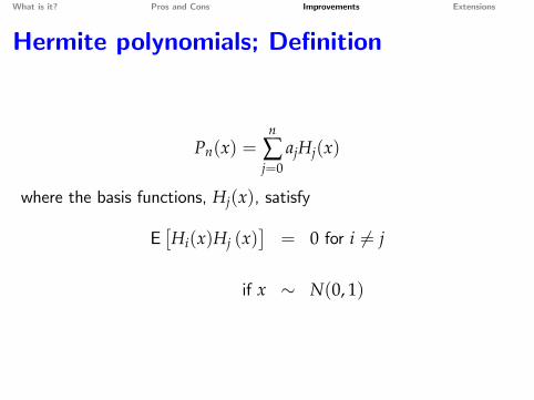
Hermite polynomials; Definition

Pn(x) =n

∑j=0

ajHj(x)

where the basis functions, Hj(x), satisfy

E[Hi(x)Hj (x)

]= 0 for i 6= j

if x ∼ N(0, 1)


Hermite polynomials; Construction

H0(x) = 1H1(x) = x

Hm+1(x) = xHm(x)−mHm−1(x) for j > 1

This gives

H0(x) = 1H1(x) = xH2(x) = x2 − 1H3(x) = x3 − 3xH4(x) = x4 − 6x2 + 3H5(x) = x5 − 10x3 + 15x


One tricky aspect about scaling

Suppose one of the explanatory variables is

xt =kt −MT

ST

MT =T

∑t=1

kt/T & ST =

(T

∑t=1(kt −M(kt)

2 /T

)1/2


One tricky aspect about scaling

• =⇒ each iteration the explanatory variables change (since Mand S change)

• =⇒ taking a weighted average of old and new coeffi cient is odd

• I found that convergence properties can be quite bad

• In principle you can avoid problem by rewriting polynomial,but that is tedious for higher-order

• So better to keep MT and ST fixed across iterations


Two graphs say it all; regular polynomials

-2 -1.5 -1 -0.5 0 0.5 1 1.5 2-30

-20

-10

0

10

20

30


Two graphs say it all; Hermite polynomials

-2 -1.5 -1 -0.5 0 0.5 1 1.5 2-20

-15

-10

-5

0

5

10

15

20


LS-Singular Values Decomposition

β =(X′X

)−1 X′Y = VS−1U′Y

• Goal: avoid calculating X′X explicitly• SVD of the (T× n) matrix X :

X = USV′

U : (T× n) orthogonal matrixS : (n× n) diagonal matrix with singular values s1 ≥ s2 ≥ · · · ≥ sn

V : (n× n) orthogonal matrix

• si is the sqrt of ith eigen value


LS-Singular Values Decomposition

In Matlab[U,S,V]=svd(X,0);


Principal components

• With many explanatory variables use principle components• SVD: X = USV′ where X is demeaned• Principle components: Z = XV• Properties Zi : mean zero and variance s2

i

• Idea: exclude principle components corresponding to lowereigenvalues

• But check with how much R2 drops


PEA and learning

• Traditional algorithm:• simulate an economy using belief ηi

n• formulate new belief ηi+1

n• simulate same economy using belief ηi+1

n


PEA and learning

• Alternative algorithm to find fixed point• simulate T observations using belief ηT−1

n• formulate new belief ηT

n• generate 1 more observation• use T+ 1 observations to formulate new belief ηT+1

• continue

• Convergence properties can be problematic


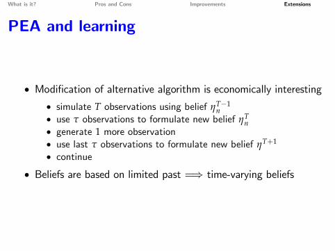
PEA and learning

• Modification of alternative algorithm is economically interesting• simulate T observations using belief ηT−1

n• use τ observations to formulate new belief ηT

n• generate 1 more observation• use last τ observations to formulate new belief ηT+1

• continue

• Beliefs are based on limited past =⇒ time-varying beliefs


PEA and learning

• Suppose the model has different regimes• e.g. high productivity and low productivity regime• agents do not observe regime=⇒ it makes sense to use limitednumber of past observations

• With the above algorithm agents gradually learn new law ofmotion


PEA and perturbation

• True in many macroeconomic models:• perturbation generates accurate solution of "real side" of theeconomy

• perturbation does not generates accurate solution of assetprices

• real side does not at all or not much depend on asset prices

• Then solve for real economy using perturbation and for assetprices using PEA

• one-step algorithm (no iteration needed)


References

• Den Haan, W.J. and A. Marcet, 1990, Solving the stochasticgrowth model with parameterized expectations, Journal of Businessand Economic Statistics.

• Den Haan, W.J., Parameterized expectations, lecture notes.• Heer, B., and A. Maussner, 2009, Dynamic General EquilibriumModeling.

• Judd, K. L. Maliar, and S. Maliar, 2011, One-node quadrature beatsMonte Carlo: A generlized stochastic simulation algorithm, NBERWP 16708

• Judd, K. L. Maliar, and S. Maliar, 2010, Numerically stablestochastic methods for solving dynamics models, NBER WP 15296

parameterized expectations algorithm - wouter den … is it?pros and consimprovementsextensions...

Documents