1

Parallel Molecular Dynamics This chapter explains the example parallel MD program, pmd.c, in detail. Spatial Decomposition • Spatial decomposition: The physical system to be simulated is partitioned into subsystems of equal

volume. Processors in a parallel computer are logically arranged according to the topology of physical subsystems. Atoms that are located in a particular subsystem are assigned to the corresponding processor.

We use a simple 3D mesh (or torus because of the periodic boundary conditions) decomposition. Subsystems are (and accordingly processors are logically) arranged in a 3D array of dimensions Px × Py × Pz (int vproc[3] in pmd.c). Each subsytem is a parallel-piped of size Lx × Ly × Lz (double al[3]). PROCESSOR ID

2

Each processor is given a unique processor ID, p, the range of which is [0, P-1] (int sid) where P = Px Py Pz is the total number of processors (int nproc). We also define a vector processor ID

€

p = (px,

py, pz) (int vid[3]), where px = 0, ..., Px-1; py = 0, ..., Py-1; and pz = 0, ..., Pz-1. The relation between the sequential and vector ID’s is px = p/(PyPz) py = (p/Pz) mod Py pz = p mod Pz or p = px×PyPz + py×Pz + pz. (Example) (Px, Py, Pz) = (4,3,2)

Sequential processor ID, p

px

Vector ID,

p

py

pz 0 1 2 3 4 5 6 7 8 9

10 11 ...

0 0 0 0 0 0 1 1 1 1 1 1 ...

0 0 1 1 2 2 0 0 1 1 2 2 ...

0 1 0 1 0 1 0 1 0 1 0 1 ...

NEIGHBOR PROCESSOR ID

For each processor, the six face-shared neighbor are identified by a sequential index (κ = 0, ..., 5). For each neighbor, κ, the shift-length vector

!Δ = (Δx, Δy, Δz) denotes the position of the neighbor

subsystem relative to itself (double sv[6][3]). The following table lists the six neighbors, where an integer vector

€

δ = (δx, δy, δz) specifies the relative location of each neighbor.

Neighbor ID, κ !δ = (δx, δy, δz)

!Δ= (Δx, Δy, Δz)

0 (east) 1 (west) 2 (north) 3 (south) 4 (up) 5 (down)

(-1, 0, 0) (1, 0, 0) (0, -1, 0) (0, 1, 0) (0, 0, -1) (0, 0, 1)

(-Lx, 0, 0) (Lx, 0, 0) (0, -Ly, 0) (0, Ly, 0) (0, 0, -Lz) (0, 0, Lz)

The sequential processor ID, p’(κ) (int nn[6]), is obtained by

p’α (κ) = [pα + δα(κ) + Pα] mod Pα (α = x, y, z) and

p’ (κ) = p’x (κ)×PyPz + p’y (κ)×Pz + p’z(κ) In an SPMD program using the MPI, each process knows its process ID through the returned rank value from an MPI_Comm_rank(MPI_Comm comm, int *rank) call. We identify the rank with sid.

3

Parallel MD Concepts Using the periodic boundary conditions, every subsystem has 26 neighbor subsystems, which share either a corner, an edge, or a face with it. (Or there are 6 face-sharing neighbor subsystems.) We express atomic coordinates relative to the origin of each subsystem, i.e., 0 < xα < Lα (α = x, y, z). (Every subsystem thinks it is the center of the world.) ATOM CACHING • Augmented system: In order to compute interatomic interaction with cut-off length rc (RCUT),

atomic coordinates of 26 neighbor subsystems which are located within rc from the subsystem boundary are copied to “this” processor (atom caching).

• Cache coherence is maintained by copying the latest neighbor surface atoms every time before

atomic accelerations are computed. DATA STRUCTURES n: The number of resident atoms which reside in “this” subsystem. nb: The number of copied surface atoms from the neighbors. r[NEMAX][3]: Atomic coordinates relative to the subsystem origin. r[0:n-1][] hold the atoms reside in this subsystem, while r[n:n+nb-1][] hold the cached neighbor atoms.

ATOM MIGRATION After the atomic coordinates are updated according to the velocity Verlet algorithm, some resident atoms may have moved out of the subsystem boundary. Such migrated atoms must be moved to proper processors.

4

PARALLEL MD ALGORITHM In the parallel MD program, pmd.c, a single time step of the velocity-Verlet algorithm consists of the following steps. 1. First half kick to obtain vi(t+Dt/2) 2. Update atomic coordinates to obtain ri(t+Dt) 3. atom_move(): Migrate the moved-out atoms to the neighbor processors 4. atom_copy(): Copy the surface atoms within distance rc from the neighbors 5. compute_accel(): Compute new accelerations, ai(t+Dt), including the contributions from the cached atoms 6. Second half kick to obtain vi(t+Dt) Linked-List Cell Method for Interatomic Force Computation function compute_accel() Recall that a naive double-loop implementation to compute pair interactions scales as O(N2). In fact, with a finite cut-off length, rc, an atom interacts with only a limited number of atoms ~ (4π/3) rc

3 (N/V). The linked-list cell algorithm computes the entire interaction with O(N) operations. CELLS First divide the system consisting of the resident and cached atoms into small cells of equal size. The edge lengths of each cell, (rcx, rcy, rcz) (double rc[3]), must be at least rc; we use rcα = Lα/Lcα, where Lcα = ⎣Lα/rc⎦. An atom in a cell interacts with only other atoms in the same cell and its 26 neighbor cells. Including the cached atoms, the range of atomic coordinates is [-rc, Lα + rc] (α = x, y, z). The number of cells to accommodate all these atoms is (Lcx+2)×(Lcy+2)×(Lcz+2), where Lcα = Lα/rcα (α = x, y, z) (int lc[3]). We identify a cell with a vector cell index, c = (cx, cy, cz) (0 ≤ cx ≤ Lcx+1; 0 ≤ cy ≤ Lcy+1; 0 ≤ cz ≤ Lcz+1), and a sequential cell index, c = cx(Lcy+2)(Lcz+2) + cy(Lcz+2) + cz or cx = c/[(Lcy+2)(Lcz+2)] cy = [c/(Lcz+2)] mod (Lcy+2) cz = c mod (Lcz+2). An atom with coordinate r belongs to a cell with the vector cell index,

cα = ⎣(rα+rcα)/rcα⎦ (α = x, y, z).

5

LISTS The atoms belonging to a cell is organized as a linked list.

DATA STRUCTURES lscl[NEMAX]: An array implementation of the linked list. lscl[i] holds the atom index to which the i-th atom points. head[NCLMAX]: head[c] holds the index of the first atom in the c-th cell, or head[c] = EMPTY (= -1) if there is no atom in the cell.

6

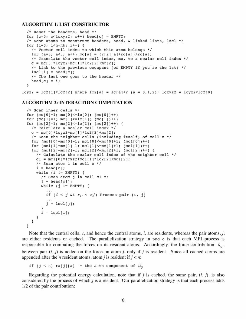
ALGORITHM 1: LIST CONSTRUCTOR /* Reset the headers, head */ for (c=0; c<lcxyz2; c++) head[c] = EMPTY; /* Scan atoms to construct headers, head, & linked lists, lscl */ for (i=0; i<n+nb; i++) { /* Vector cell index to which this atom belongs */ for (a=0; a<3; a++) mc[a] = (r[i][a]+rc[a])/rc[a]; /* Translate the vector cell index, mc, to a scalar cell index */ c = mc[0]*lcyz2+mc[1]*lc2[2]+mc[2]; /* Link to the previous occupant (or EMPTY if you're the 1st) */ lscl[i] = head[c]; /* The last one goes to the header */ head[c] = i; }

lcyz2 = lc2[1]*lc2[2] where lc2[a] = lc[a]+2 (a = 0,1,2); lcxyz2 = lcyz2*lc2[0] ALGORITHM 2: INTERACTION COMPUTATION /* Scan inner cells */ for (mc[0]=1; mc[0]<=lc[0]; (mc[0])++) for (mc[1]=1; mc[1]<=lc[1]; (mc[1])++) for (mc[2]=1; mc[2]<=lc[2]; (mc[2])++) { /* Calculate a scalar cell index */ c = mc[0]*lcyz2+mc[1]*lc2[2]+mc[2]; /* Scan the neighbor cells (including itself) of cell c */ for (mc1[0]=mc[0]-1; mc1[0]<=mc[0]+1; (mc1[0])++) for (mc1[1]=mc[1]-1; mc1[1]<=mc[1]+1; (mc1[1])++) for (mc1[2]=mc[2]-1; mc1[2]<=mc[2]+1; (mc1[2])++) { /* Calculate the scalar cell index of the neighbor cell */ c1 = mc1[0]*lcyz2+mc1[1]*lc2[2]+mc1[2]; /* Scan atom i in cell c */ i = head[c]; while (i != EMPTY) { /* Scan atom j in cell c1 */ j = head[c1]; while (j != EMPTY) { ... if (i < j && rij < rc

2) Process pair (i, j) ... j = lscl[j]; } i = lscl[i]; } } }

Note that the central cells, c, and hence the central atoms, i, are residents, whereas the pair atoms, j, are either residents or cached. The parallelization strategy in pmd.c is that each MPI process is responsible for computing the forces on its resident atoms. Accordingly, the force contribution, aij , between pair (i, j) is added on the force on atom j, only if j is resident. Since all cached atoms are appended after the n resident atoms, atom j is resident if j < n:

if (j < n) ra[j][a] -= the a-th component of aij

Regarding the potential energy calculation, note that if j is cached, the same pair, (i, j), is also considered by the process of which j is a resident. Our parallelization strategy is that each process adds 1/2 of the pair contribution:

7

if (j < n) potential energy += u(rij ); else potential energy += u(rij )/2;

Note that each process first computes the local contribution to the potential energy, and subsequently MPI_Allreduce() is used to compute the global summation of the local potential energies. Atom Caching—function atom_copy() DATA STRUCTURES lsb[6][NBMAX]: lsb[ku][0] is the total number of boundary atoms to be sent to neighbor ku; lsb[ku][k] is the atom ID, used in r, of the k-th atom to be sent. logical function bbd(r,ku): true if the coordinate vector r is within distance rc from the face this subsystem shares with the ku-th neighbor. The coordinates of the boundary atoms to the six face-sharing neighbors are sent to these nodes in six steps. Copies to the non-face-sharing neighbors (26 − 6 = 20) are done by message forwarding.

ALGORITHM Reset the number of received cache atoms, nbnew = 0 for x, y, and z directions Make boundary-atom lists, lsb, for lower and higher directions including both resident, n, and cache, nbnew, atoms for lower and higher directions* Send/receive boundary-atom coordinates to/from the neighbor# Increment nbnew endfor endfor nb = nbnew

*Copying condition bbd(ri[],ku) { kd = ku / 2 (= 0|1|2) kdd = ku % 2 (= 0|1) if (kdd == 0) return ri[kd] < RCUT else return al[kd] – RCUT < ri[kd] }

#Three-phase message passing 1. Message buffering: dbuf ← r-sv (shift positions), gather 2. Message passing: dbufr ← dbuf

Send dbuf Receive dbufr

3. Message storing: r ← dbufr, append after the residents

8

Variable nsd is the number of atoms to be copied to the neighbor currently considered. The 3*nsd coordinates are packed in a 1D array, dbuf.

DEADLOCK AVOIDANCE A circular send and receive relation could cause a deadlock. (Circular wait can occur if blocking.) In the following code, suppose that the destination node, inode, is defined as in the figure below. MPI_Send(dbuf,3*nsd,MPI_DOUBLE_PRECISON,inode,10,MPI_COMM_WORLD); MPI_Recv(dbufr,3*nrc,MPI_ DOUBLE_PRECISON,MPI_ANY_SOURCE,10,MPI_COMM_WORLD,&status);

With a finite buffer size in the receiver’s communication system, a sender blocks until the receiver’s buffer is cleared. However in the example above, each processor cannot start receiving until its send operation is completed.

To avoid this deadlock, we classify the processors into even and odd processors in each of the x, y, and z directions.

9

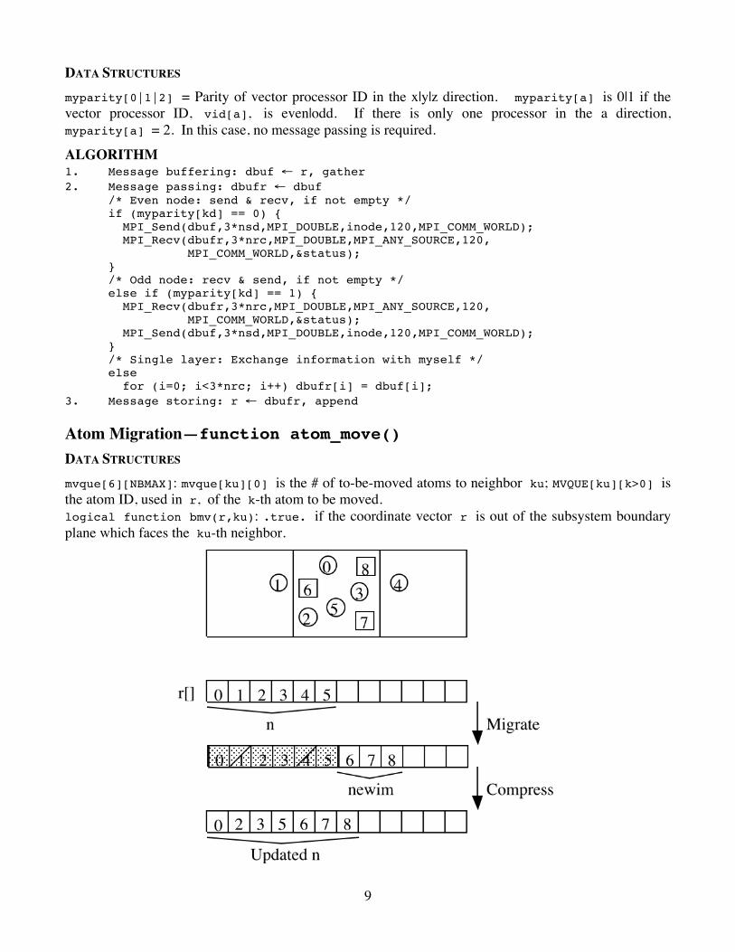
DATA STRUCTURES myparity[0|1|2] = Parity of vector processor ID in the x|y|z direction. myparity[a] is 0|1 if the vector processor ID, vid[a], is even|odd. If there is only one processor in the a direction, myparity[a] = 2. In this case, no message passing is required.

ALGORITHM 1. Message buffering: dbuf ← r, gather 2. Message passing: dbufr ← dbuf /* Even node: send & recv, if not empty */ if (myparity[kd] == 0) { MPI_Send(dbuf,3*nsd,MPI_DOUBLE,inode,120,MPI_COMM_WORLD); MPI_Recv(dbufr,3*nrc,MPI_DOUBLE,MPI_ANY_SOURCE,120, MPI_COMM_WORLD,&status); } /* Odd node: recv & send, if not empty */ else if (myparity[kd] == 1) { MPI_Recv(dbufr,3*nrc,MPI_DOUBLE,MPI_ANY_SOURCE,120, MPI_COMM_WORLD,&status); MPI_Send(dbuf,3*nsd,MPI_DOUBLE,inode,120,MPI_COMM_WORLD); } /* Single layer: Exchange information with myself */ else for (i=0; i<3*nrc; i++) dbufr[i] = dbuf[i]; 3. Message storing: r ← dbufr, append Atom Migration—function atom_move() DATA STRUCTURES mvque[6][NBMAX]: mvque[ku][0] is the # of to-be-moved atoms to neighbor ku; MVQUE[ku][k>0] is the atom ID, used in r, of the k-th atom to be moved. logical function bmv(r,ku): .true. if the coordinate vector r is out of the subsystem boundary plane which faces the ku-th neighbor.

10

The algorithm is basically the same as the one in atom_copy. During the 6-step loop, variable newim keeps the number of received new immigrants. These atoms are appended in the r array after the current resident. Suppose atom i has moved-out. When sending out r[i] to a proper neighbor, r[i] is marked as moved-out by putting constant MOVED_OUT (large negative value, -1e10, defined in pmd.h) in r[i][0]. When scanning n+newim atoms to sort out the moved-out atoms, these already-moved atoms are not considered. After the six move steps, the r array is compressed to remove the moved-out atoms. ALGORITHM Reset the number of received new immigrants, newim = 0 for x, y, and z directions Make moving-atom lists, mvque, for lower and higher directions including both resident, n, and immigrant, newim, atoms but excluding those already moved out for lower and higher directions* Send/receive moving-atom coordinates to/from the neighbor# (When moving, r[][0] ← MOVED_OUT = -1010) Increment newim endfor endfor Compress the r array to eliminate the moved-out atoms

*Moving condition bmv(ri[],ku) { kd = ku / 2 (= 0|1|2) kdd = ku % 2 (= 0|1) if (kdd == 0) return ri[kd] < 0.0 else return al[kd] < ri[kd] }

#Three-phase message passing 1. Message buffering: dbuf ← r & rv, gather

Mark MOVED_OUT in r 2. Message passing: dbufr ← dbuf

Send dbuf Receive dbufr

3. Message storing: r & rv ← dbufr, append after the residents

11

Scalability Metrics for Parallel Molecular Dynamics Parallel Efficiency

We define the efficiency of a parallel program running on P processors to solve a problem of size W. Let T(W, P) be the execution time of this parallel program. Speed of the program is then S(W, P) = W/T(W, P). Speedup, SP, on P processors is the speed of P processors divided by that of 1 processor, i.e., SP = S(WP, P)/S(W1, 1). To unambiguously define the speedup, we need to specify how the problem size, WP, scales as a function of the number of processors, P (which will be discussed in the next few paragraphs). The ideal speedup on P processors is expected to be P, and therefore we define the parallel efficiency, EP = SP/P. CONSTANT PROBLEM-SIZE SCALING

In the constant problem-size scaling, the problem size WP = W is fixed constant. Therefore, the constant problem-size speedup is

SP =S(W,P)

S(W,1)=W /T (W,P)

W /T (W,1)=T (W,1)

T (W,P),

and the parallel efficiency is

EP =SP

P=

T (W,1)

P•T (W,P).

Amdahl’s law: Consider a case, in which a fraction, f (∈ [0, 1]), of the work W is inherently sequential and cannot be parallelized, but the rest, 1 − f, can be divided and executed in parallel on P processors. Then, T(W, P) = f•T(W, 1) + (1 − f)T(W, 1)/P. Therefore, the speedup is

SP =T (W,1)

T (W,P)=

1

f + (1− f ) / P.

In the limit of large number of processors, P → ∞, the asymptotic speedup is SP → 1/f. The constant problem-size speedup is thus limited by the fraction of the sequential bottleneck of the parallel program. For example, if 1% of the work is sequential, the maximum achievable speedup is 0.01/1 = 100, and it does not make sense to use more than ~100 processors to run this program. ISOGRANULAR SCALING

In the isogranular scaling, the problem size WP scales linearly with the number of processors: WP = P•w, where the granularity (or the work per processor), w, is constant. Therefore, the isogranular speedup is

SP =S(P•w,P)S(w,1)

=P•w /T (P•w,P)

w /T (w,1)=P•T (w,1)T (P•w,P)

,

and the corresponding isogranular parallel efficiency is

EP =SP

P=

T (w,1)

T (P•w,P).

12

Analysis of Parallel Molecular Dynamics Algorithm

Using the spatial decomposition and the O(N) linked-list cell method, the parallel MD simulation of N atoms executes independently on P processors, and the computation time Tcomp(N, P) = aN/P, where a is a constant. Here, we have assumed that atoms are on average distributed uniformly, so that the average number of atoms per processor is N/P. The dominant overhead of the parallel MD is atom caching, in which atoms near the subsystem boundary within a cutoff distance, rc, are copied from the nearest neighbor processors and are processed. Since this nearest-neighbor communication scales as the surface area of each spatial subsystem, its time is Tcomm(N, P) = b(N/P)2/3, where b is a constant. Another major communication cost is for global summations, MPI_Allreduce(), which incurs Tglobal(P) = c logP, where c is another constant.

The total execution time of the parallel MD program can thus be modeled as

T (N,P) = Tcomp(N,P)+Tcomm(N,P)+Tglobal(P)

= aN / P + b(N / P)2/3 + c logP.

CONSTANT PROBLEM-SIZE SCALING For constant problem-size scaling, the global number of atoms, N, is fixed, and the speedup is given

by

SP =T (N,1)T (N,P)

=aN

aN / P + b(N / P)2/3 + c logP

=P

1+ ba

PN!

"#

$

%&1/3

+caP logPN

,

and the parallel efficiency is

EP =SPP=

1

1+ ba

PN!

"#

$

%&1/3

+caP logPN

.

From this model, we can see that the efficiency is a decreasing function of P through both the P1/3 and PlogP dependences. ISOGRANULAR SCALING

For isogranular scaling, the number of atoms per processor, N/P = n, is constant, and the isogranular parallel efficiency is

EP =T (n,1)T (nP,P)

=an

an+ bn2/3 + c logP=

1

1+ ban−1/3 + c

anlogP

.

For a given number of processors, the efficiency EP is larger for larger granularity n. For a given granularity, EP is a weakly decreasing function of P, due to only the logP dependence.