4. molecular dynamics - acmm · understanding molecular simulation 76 chapter 3. molecular dynamics...

Understanding Molecular Simulation

4. Molecular dynamics


Molecular Simulations

➡ Molecular dynamics: solve equations of motion

➡ Monte Carlo: importance sampling

r1r2rn

r1r2rn


Molecular Dynamics4. Molecular Dynamics

4.1.Introduction 4.2.Basics 4.3.Liouville formulation 4.4.Multiple time steps



4.2 Basics


“Fundamentals”

Theory:

• Compute the forces on the particles • Solve the equations of motion • Sample after some # of timesteps

F =md2rdt2



4.3 Some practical details


Initialization • Total momentum should be zero (no external forces) • Temperature rescaling to desired temperature • Particles start on a lattice

Force calculations • Periodic boundary conditions • Order NxN algorithm, • Order N: neighbor lists, linked cell • Truncation and shift of the potential

Integrating the equations of motion • Velocity Verlet • Kinetic energy

Molecular Dynamics


Molecular Dynamics3.2 Molecular Dynamics: A Program 75

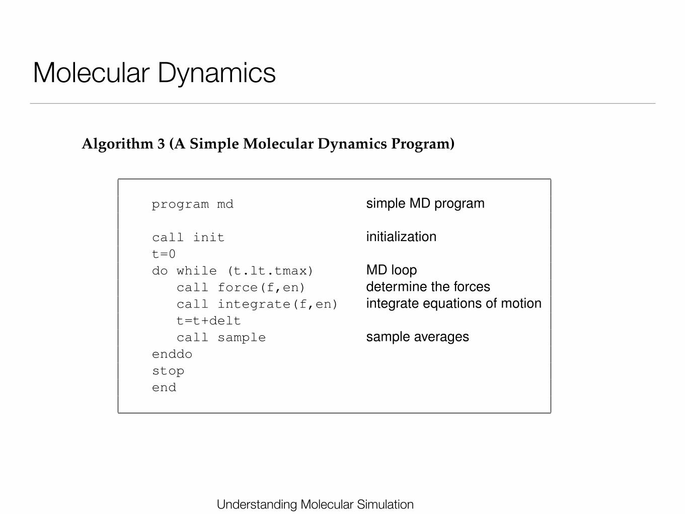
Algorithm 3 (A Simple Molecular Dynamics Program)

program md simple MD program

call init initializationt=0

do while (t.lt.tmax) MD loopcall force(f,en) determine the forcescall integrate(f,en) integrate equations of motiont=t+delt

call sample sample averagesenddo

stop

end

Comment to this algorithm:

1. Subroutines init, force, integrate, and sample will be described inAlgorithms 4, 5, and 6, respectively. Subroutine sample is used to calculateaverages like pressure or temperature.

2. We initialize the system (i.e., we select initial positions and velocities).3. We compute the forces on all particles.4. We integrate Newton’s equations of motion. This step and the previ-

ous one make up the core of the simulation. They are repeated until wehave computed the time evolution of the system for the desired lengthof time.

5. After completion of the central loop, we compute and print the aver-ages of measured quantities, and stop.

Algorithm 3 is a short pseudo-algorithm that carries out a Molecular Dy-namics simulation for a simple atomic system. We discuss the different op-erations in the program in more detail.

3.2.1 InitializationTo start the simulation, we should assign initial positions and velocities to allparticles in the system. The particle positions should be chosen compatiblewith the structure that we are aiming to simulate. In any event, the particlesshould not be positioned at positions that result in an appreciable overlapof the atomic or molecular cores. Often this is achieved by initially placing

Understanding Molecular Simulation (DRAFT - 3rd edition) Frenkel and Smit (November 7, 2017)


3. Molecular dynamics: practical details

3.3.1 Initialization


76 Chapter 3. Molecular Dynamics Simulations

Algorithm 4 (Initialization of a Molecular Dynamics Program)

subroutine init initialization of MD programsumv=0

sumv2=0

do i=1,npart

x(i)=lattice pos(i) place the particles on a latticev(i)=(ranf()-0.5) give random velocitiessumv=sumv+v(i) velocity center of masssumv2=sumv2+v(i)**2 kinetic energy

enddo

sumv=sumv/npart velocity center of masssumv2=sumv2/npart mean-squared velocityfs=sqrt(3*temp/sumv2) scale factor of the velocitiesdo i=1,npart set desired kinetic energy and set

v(i)=(v(i)-sumv)*fs velocity center of mass to zeroxm(i)=x(i)-v(i)*dt position previous time step

enddo

return

end

Comments to this algorithm:

1. Function lattice pos gives the coordinates of lattice position i andranf() gives a uniformly distributed random number. We do not use aMaxwell-Boltzmann distribution for the velocities; on equilibration it will be-come a Maxwell-Boltzmann distribution.

2. In computing the number of degrees of freedom, we assume a three-di-mensional system (in fact, we approximate Nf by 3N).

the particles on a cubic lattice, as described in section 2.2.2 in the context ofMonte Carlo simulations.

In the present case (Algorithm 4), we have chosen to start our run froma simple cubic lattice. Assume that the values of the density and initial tem-perature are chosen such that the simple cubic lattice is mechanically un-stable and melts rapidly. First, we put each particle on its lattice site andthen we attribute to each velocity component of every particle a value thatis drawn from a uniform distribution in the interval [-0.5, 0.5]. This initialvelocity distribution is Maxwellian neither in shape nor even in width. Sub-sequently, we shift all velocities, such that the total momentum is zero andwe scale the resulting velocities to adjust the mean kinetic energy to the de-

Understanding Molecular Simulation (DRAFT - 3rd edition) Frenkel and Smit (November 7, 2017)



3.3.2 Force calculation


Periodic boundary conditions


The Lennard-Jones potentials

• The Lennard-Jones potential

• The truncated Lennard-Jones potential

• The truncated and shifted Lennard-Jones potential

ULJ r( ) = 4ε σr

⎛⎝⎜

⎞⎠⎟

12

− σr

⎛⎝⎜

⎞⎠⎟

6⎡

⎣⎢⎢

⎤

⎦⎥⎥

UTRLJ r( ) = ULJ r( ) r ≤ rc

0 r > rc

⎧⎨⎪

⎩⎪

UTR−SHLJ r( ) = ULJ r( )−ULJ rc( ) r ≤ rc

0 r > rc

⎧⎨⎪

⎩⎪


The Lennard-Jones potentials


Saving CPU-time

Cell list Verlet-list



3.3.3 Equations of motion


70 Chapter 4. Molecular Dynamics Simulations

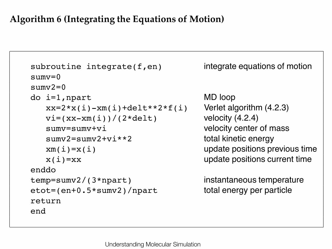
Algorithm 6 (Integrating the Equations of Motion)

subroutine integrate(f,en) integrate equations of motionsumv=0sumv2=0do i=1,npart MD loop

xx=2*x(i)-xm(i)+delt**2*f(i) Verlet algorithm (4.2.3)vi=(xx-xm(i))/(2*delt) velocity (4.2.4)sumv=sumv+vi velocity center of masssumv2=sumv2+vi**2 total kinetic energyxm(i)=x(i) update positions previous timex(i)=xx update positions current time

enddotemp=sumv2/(3*npart) instantaneous temperatureetot=(en+0.5*sumv2)/npart total energy per particlereturnend

Comments to this algorithm:

1. The total energy etot should remain approximately constant during the sim-ulation. A drift of this quantity may signal programming errors. It thereforeis important to monitor this quantity. Similarly, the velocity of the center ofmass sumv should remain zero.

2. In this subroutine we use the Verlet algorithm (4.2.3) to integrate the equa-tions of motion. The velocities are calculated using equation (4.2.4).

similarly,

Summing these two equations, we obtain

or(4.2.3)

The estimate of the new position contains an error that is of order ,where is the time step in our Molecular Dynamics scheme. Note that the


Equations of motion

r t + Δt( ) = r t( )+ dr t( )dt

Δt +d2r t( )dt2

Δt2

2!+O Δt3( )

We can make a Taylor expansion for the positions:

The simplest form (Euler):

v t + Δt( ) = v t( )+mdf t( )dt

Δt

r t + Δt( ) = r t( )+ v t( )Δt +O Δt2( )

We can do better!


r t + Δt( ) = r t( )+ dr t( )dt

Δt +d2r t( )dt2

Δt2

2!+d2r t( )dt2

Δt3

3!+O Δt4( )

We can make a Taylor expansion for the positions:

When we add the two:

Verlet algorithm

r t − Δt( ) = r t( )− dr t( )dt

Δt +d2r t( )dt2

Δt2

2!−d2r t( )dt2

Δt3

3!+O Δt4( )

r t + Δt( )+ r t − Δt( ) = 2r t( )+ d2r t( )dt2

Δt2 +O Δt4( )

r t + Δt( ) = 2r t( )− r t − Δt( )+ f t( )Δt2

m+O Δt4( )

no need for velocitiesnumerically not

ideal


Velocity Verlet algorithm

Verlet algorithm:

v t + Δt( ) = v t( )+ Δt2mf t + Δt( )+ f t( )⎡⎣ ⎤⎦

r t + Δt( ) = 2r t( )− r t − Δt( )+ f t( )Δt2

m+O Δt4( )

r t + Δt( ) = r t( )+ v t( )Δt + f t( )Δt2

2m+O Δt4( )

to see the equivalence:

r t +2Δt( ) = 2r t + Δt( )− r t( )+ v t + Δt( )− v t( )⎡⎣ ⎤⎦Δt + f t + Δt( )− f t( )⎡⎣ ⎤⎦Δt2

2m

r t( ) = r t + Δt( )− v t( )Δt − f t( )Δt2

2m

r t +2Δt( ) = r t + Δt( )+ v t + Δt( )Δt + f t + Δt( )Δt2

2m

adding the two

with v t + Δt( ) = v t( )+ Δt2mf t + Δt( )+ f t( )⎡⎣ ⎤⎦

r t +2Δt( ) = 2r t + Δt( )− r t( )+ f t + Δt( )Δt2

m


Lyaponov instability

r1 0( ),!,rN 0( ),p1 0( ),!,pN 0( )( )MD: reference trajectory with initial condition:MD: compare: r1 0( ),!,rN 0( ),p1 0( ),!,pi 0( )+ ε ,pj 0( )− ε ,!,pN 0( )( )

ε = 10−10


4. Molecular dynamics:

4.4 Liouville Formulation


the dot above, ḟ, implies time derivative Liouville formulation

Let us consider a function that f which depends on the positions and momenta of the particles: f pN ,rN( )

!f = ∂f∂r

⎛⎝⎜

⎞⎠⎟!r + ∂f

∂p⎛⎝⎜

⎞⎠⎟!p

We can “solve” how f depends on time:

Define the Liouville operator:iL ≡ !r ∂

∂r⎛⎝⎜

⎞⎠⎟+ !p ∂

∂p⎛⎝⎜

⎞⎠⎟

the time dependence follows from: dfdt

= iLfwith solution:

f = eiLtf 0( )beware: the solution is equally useless as the differential equation


In an ideal world it would be less useless:iL ≡ !r ∂

∂r⎛⎝⎜

⎞⎠⎟+ !p ∂

∂p⎛⎝⎜

⎞⎠⎟

Let us look at half the equation iLr ≡∂∂r

⎛⎝⎜

⎞⎠⎟!r

f = eiLrtf 0( )which has as solution:

ex = 1 + x + x2

2!+ x

3

3!+!Taylor expansion:

eiLrtf 0( ) = 1 + iLrt + 12 iLrt( )2 + 13! iLrt( )3 +…⎡

⎣⎢

⎤

⎦⎥f 0( )

eiLrtf 0( ) = 1 + !r 0( )t ∂∂r

⎛⎝⎜

⎞⎠⎟+ 12!r 0( )t( )2 ∂

∂r⎛⎝⎜

⎞⎠⎟

2

+…⎡

⎣⎢⎢

⎤

⎦⎥⎥f 0( )

f 0+ !r 0( )t( ) = f 0( )+ !r 0( )t ∂f 0( )∂r

⎛

⎝⎜

⎞

⎠⎟ +12!r 0( )t( )2 ∂f 0( )

∂r

⎛

⎝⎜

⎞

⎠⎟

2

+!

Hence: eiLrtf 0( ) = f 0+ !r 0( )t( )

the operator iLr gives a shift of the positions


The operation iLr gives a shift of the positionsiL ≡ !r ∂

∂r⎛⎝⎜

⎞⎠⎟+ !p ∂

∂p⎛⎝⎜

⎞⎠⎟

Similarly for the operator iLp iLp ≡∂∂p

⎛⎝⎜

⎞⎠⎟!p

f = eiLptf 0( )which has as solution:

Taylor expansion:

eiLptf 0( ) = 1 + iLpt + 12 iLpt( )2 + 13! iLpt( )3 +…⎡

⎣⎢

⎤

⎦⎥f 0( )

eiLptf 0( ) = 1 + !p 0( )t ∂∂p

⎛⎝⎜

⎞⎠⎟+ 12!p 0( )t( )2 ∂

∂p⎛⎝⎜

⎞⎠⎟

2

+…⎡

⎣⎢⎢

⎤

⎦⎥⎥f 0( )

f 0+ !p 0( )t( ) = f 0( )+ !p 0( )t ∂f 0( )∂p

⎛

⎝⎜

⎞

⎠⎟ +12!p 0( )t( )2 ∂f 0( )

∂p

⎛

⎝⎜

⎞

⎠⎟

2

+!

Hence: eiLptf 0( ) = f 0+ !p 0( )t( )

the operator iLp gives a shift of the momenta


The operation iLr gives a shift of the positions:

… and the operator iLp a shift of the momenta:

This would have been useful if the operators would commute

eiLtf 0,0( ) = e iLr+iLp( )tf 0,0( ) ≠ eiLrteiLptf 0,0( )

eiLrtf 0,0( ) = f 0,0+ !r 0( )t( )

eiLptf 0,0( ) = f 0+ !p 0( )t,0( )

Trotter expansion:

eA+B ≠ eAeBwe have the non-commuting operators A and B:

then the following expansion holds:

eA+B = limP→∞ eA2Pe

BPe

A2P( )P


We can apply the Trotter expansion:

eiLrΔtf p t( ),r t( )( ) = f p t( ),r t( )+ !r t( )Δt( )

eiLptf 0,0( ) = f 0+ !p 0( )t,0( )eA+B = limP→∞ e

A2Pe

BPe

A2P( )P

Δt = tP

iLrtP

= iLrΔtiLpt2P

= iLpΔt2

eiLpΔt 2f p t( ),r t( )( ) = f p t( )+ !p t( )Δt2 ,r t( )⎛⎝⎜

⎞⎠⎟

gives us a shift of the position: r t + Δt( )→ r t( )+ !r t( )Δt

gives us a shift of the momenta: p t + Δt( )→ p t( )+ !p t( )Δt2

eiLrtf 0,0( ) = f 0,0+ !r 0( )t( )

These give as operations:


We can apply the Trotter expansion to integrate M time steps: t=M x Δt

eiLpΔt2

f t( ) = eiLtf 0( ) = eiLp Δt2eiLrΔteiLp Δt2( )M f 0( )

iLrΔt

iLpΔt2

r t + Δt( )→ r t( )+ !r t( )Δtp t + Δt

2⎛⎝⎜

⎞⎠⎟→ p t( )+ !p t( )Δt2

These give as operations:

p Δt2

⎛⎝⎜

⎞⎠⎟→ p 0( )+ !p 0( )Δt2

eiLpΔt2

eiLrΔt r Δt( )→ r 0( )+ !r Δt2

⎛⎝⎜

⎞⎠⎟Δt

p Δt( )→ p Δt2

⎛⎝⎜

⎞⎠⎟+ !p Δt( )Δt2which gives after one step

p 0( )→ p 0( )+ f 0( )+ f Δt( )⎡⎣ ⎤⎦Δt2

r 0( )→ r 0( )+ !r Δt2

⎛⎝⎜

⎞⎠⎟Δt = r 0( )+ v 0( )Δt + f 0( )Δt

2

2m


which gives after one step

p 0( )→ p 0( )+ f 0( )+ f Δt( )⎡⎣ ⎤⎦Δt2

r 0( )→ r 0( )+ !r Δt2

⎛⎝⎜

⎞⎠⎟Δt = r 0( )+ v 0( )Δt + f 0( )Δt

2

2m

Velocity Verlet algorithmr t + Δt( ) = r t( )+ v t( )Δt + f t( )Δt

2

2m

v t + Δt( ) = v t( )+ Δt2mf t + Δt( )+ f t( )⎡⎣ ⎤⎦


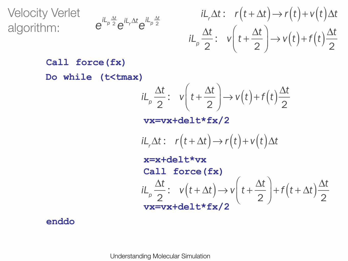
vx=vx+delt*fx/2

x=x+delt*vxCall force(fx)

vx=vx+delt*fx/2

Call force(fx)Do while (t<tmax)

enddo

Velocity Verlet algorithm: eiLp

Δt2eiLrΔteiLp

Δt2

iLrΔt : r t + Δt( )→ r t( )+ v t( )Δt

iLpΔt2: v t + Δt

2⎛⎝⎜

⎞⎠⎟→ v t( )+ f t( )Δt2

iLpΔt2: v t + Δt

2⎛⎝⎜

⎞⎠⎟→ v t( )+ f t( )Δt2

iLrΔt : r t + Δt( )→ r t( )+ v t( )Δt

iLpΔt2: v t + Δt( )→ v t + Δt

2⎛⎝⎜

⎞⎠⎟+ f t + Δt( )Δt2


Liouville formulation

Velocity Verlet algorithm r t + Δt( ) = r t( )+ v t( )Δt + f t( )Δt2

2mv t + Δt( ) = v t( )+ Δt

2mf t + Δt( )+ f t( )⎡⎣ ⎤⎦

Transformations:iLp Δt 2 : r t( )→ r t( )

v t( )→ v t( )+ f t( )Δt 2m

Jp = Det1 0

∂f∂r

⎛⎝⎜

⎞⎠⎟Δt2m

1= 1

iLrΔt : r t + Δt( )→ r t( )+ v t( )Δtv t( )→ v t( )Jr = Det

1 Δt0 1

= 1

Three subsequent coordinate transformations in either r or r of which the Jacobian is one: Area preserving


4. Molecular dynamics:

4.5 Multiple time steps


Multiple time steps

What to do with “stiff” potentials?

• Fixed bond-length: constraints (Shake) • Very small time step


We can split the force is the stiff part and the more slowly changing rest of the forces:

This allows us to split the Liouville operator:

Now we can make another Trotter expansion: δt=Δt/m

iLrΔt : r t + Δt( )→ r t( )+ v t( )ΔtiLp

Δt2: v t + Δt

2⎛⎝⎜

⎞⎠⎟→ v t( )+ f t( )Δt2

f t( ) = fShort t( )+ fLong t( )

iLt = iLrt + iLpShortt + iLpLong

The conventional Trotter expansion:

iLt = iLpLong Δt 2 iLr + iLpShort⎡⎣ ⎤⎦Δt iLpLong Δt 2⎡⎣

⎤⎦M

iLr + iLpShort⎡⎣ ⎤⎦Δt = iLpShort δ t 2 iLrδ t iLpShort δ t 2⎡⎣ ⎤⎦m


The algorithm to solve the equations of motion

The steps are first iLpLong then m times iLpShort/iLr followed by iLpLong again

f t( ) = fShort t( )+ fLong t( )

We now have 3 transformations:

iLt = iLpLong Δt 2 iLr + iLpShort⎡⎣ ⎤⎦Δt iLpLong Δt 2⎡⎣

⎤⎦M

iLr + iLpShort⎡⎣ ⎤⎦Δt = iLpShort δ t 2 iLrδ t iLpShort δ t 2⎡⎣ ⎤⎦m

iLpLongΔt2: v t + Δt

2⎛⎝⎜

⎞⎠⎟→ v t( )+ fLong t( )Δt2

iLpShortδ t2: v t + δ t

2⎛⎝⎜

⎞⎠⎟→ v t( )+ fShort t( )δ t2

iLrδ t : r t +δ t( )→ r t( )+ v t( )δ t


vx=vx+ddelt*fx_short/2

x=x+ddelt*vxCall force_short(fx_short)

vx=vx+ddelt*fx_short/2

Call force(fx_long,f_short)

Do ddt=1,n

enddo

vx=vx+delt*fx_long/2

iLpLongΔt2: v t + Δt

2⎛⎝⎜

⎞⎠⎟→ v t( )+ fLong t( )Δt2


2⎛⎝⎜

⎞⎠⎟→ v t( )+ fShort t( )δ t2

iLrδ t : r t +δ t( )→ r t( )+ v t( )δ t


2⎛⎝⎜

⎞⎠⎟→ v t( )+ fShort t( )δ t2

4. molecular dynamics - acmm · understanding molecular simulation 76 chapter 3. molecular dynamics...

Documents