molecular dynamics – numerics

Scientific Computing II

Molecular Dynamics – Numerics

Michael Bader – SCCSTechnical University of Munich

Summer 2017

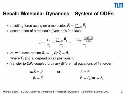
Recall: Molecular Dynamics – System of ODEs

• resulting force acting on a molecule: ~Fi =∑

j 6=i~Fij

• acceleration of a molecule (Newton’s 2nd law):

~ri =~Fi

mi=

∑j 6=i~Fij

mi= −

∑j 6=i

∂U(~ri ,~rj )∂|rij |

mi

• or, with acceleration ~ai := 1mi~Fi : ~ri = ~ai ,

where ~Fi and ~ai depend on all positions ~ri

• transfer to 2dN coupled ordinary differential equations of 1st order:

mi~ri = ~pi or ~ri = ~vi

~pi = ~Fi ~vi = ~Fi/mi = ~ai

Michael Bader – SCCS | Scientific Computing II | Molecular Dynamics – Numerics | Summer 2017 2

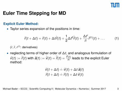
Euler Time Stepping for MD

Explicit Euler Method:• Taylor series expansion of the positions in time:

~r(t + ∆t) = ~r(t) + ∆t~r(t) +12

∆t2~r(t) +∆t i

i!~r (i)(t) + . . . (1)

(r , r , r (i): derivatives)

• neglecting terms of higher order of ∆t , and analogous formulation of~v(t) := ~r(t) with ~a(t) := ~v(t) = ~r(t) =

~F (t)m leads to the explicit Euler

method:

~v(t + ∆t) .= ~v(t) + ∆t ~a(t)

~r(t + ∆t) .= ~r(t) + ∆t ~v(t)


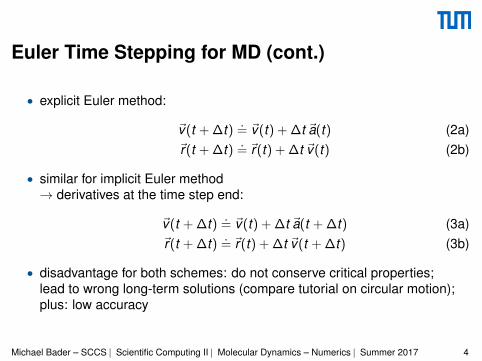
Euler Time Stepping for MD (cont.)

• explicit Euler method:

~v(t + ∆t) .= ~v(t) + ∆t ~a(t) (2a)

~r(t + ∆t) .= ~r(t) + ∆t ~v(t) (2b)

• similar for implicit Euler method→ derivatives at the time step end:

~v(t + ∆t) .= ~v(t) + ∆t ~a(t + ∆t) (3a)

~r(t + ∆t) .= ~r(t) + ∆t ~v(t + ∆t) (3b)

• disadvantage for both schemes: do not conserve critical properties;lead to wrong long-term solutions (compare tutorial on circular motion);plus: low accuracy


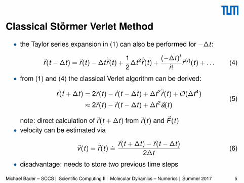
Classical Stormer Verlet Method

• the Taylor series expansion in (1) can also be performed for −∆t :

~r(t −∆t) = ~r(t)−∆t~r(t) +12

∆t2~r(t) +(−∆t)i

i!~r (i)(t) + . . . (4)

• from (1) and (4) the classical Verlet algorithm can be derived:

~r(t + ∆t) = 2~r(t)−~r(t −∆t) + ∆t2~r(t) +O(∆t4)

≈ 2~r(t)−~r(t −∆t) + ∆t2~a(t)(5)

note: direct calculation of ~r(t + ∆t) from ~r(t) and ~F (t)• velocity can be estimated via

~v(t) = ~r(t) .=~r(t + ∆t)−~r(t −∆t)

2∆t(6)

• disadvantage: needs to store two previous time steps


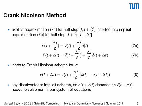
Crank Nicolson Method

• explicit approximation (7a) for half step [t , t + ∆t2 ] inserted into implicit

approximation (7b) for half step [t + ∆t2 , t + ∆t ]

~v(t +∆t2

) = ~v(t) +∆t2~a(t) (7a)

~v(t + ∆t) = ~v(t +∆t2

) +∆t2~a(t + ∆t) (7b)

• leads to Crank-Nicolson scheme for v :

~v(t + ∆t) = ~v(t) +∆t2(~a(t) + ~a(t + ∆t)

)(8)

• key disadvantage: implicit scheme, as ~a(t + ∆t) depends on ~r(t + ∆t);needs to solve non-linear system of equations


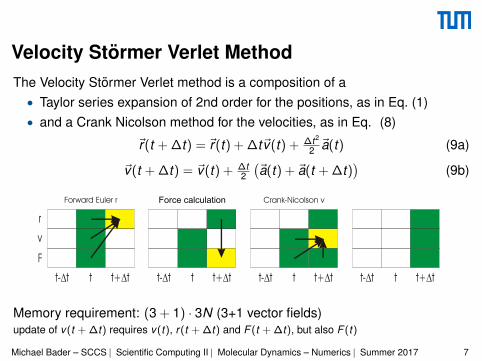
Velocity Stormer Verlet MethodThe Velocity Stormer Verlet method is a composition of a• Taylor series expansion of 2nd order for the positions, as in Eq. (1)• and a Crank Nicolson method for the velocities, as in Eq. (8)

~r(t + ∆t) = ~r(t) + ∆t~v(t) + ∆t2

2~a(t) (9a)

~v(t + ∆t) = ~v(t) + ∆t2

(~a(t) + ~a(t + ∆t)

)(9b)

tt-Dt t+Dt tt-Dt t+Dt tt-Dt t+Dt

r

v

F

tt-Dt t+Dt

Forward Euler r Force calculation Crank-Nicolson v

Memory requirement: (3 + 1) · 3N (3+1 vector fields)update of v(t + ∆t) requires v(t), r(t + ∆t) and F (t + ∆t), but also F (t)


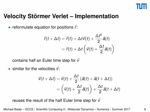
Velocity Stormer Verlet – Implementation

• reformulate equation for positions ~r :

~r(t + ∆t) = ~r(t) + ∆t~v(t) +∆t2

2~a(t)

= ~r(t) + ∆t(~v(t) +

∆t2~a(t)

)contains half an Euler time step for ~v

• similar for the velocities ~v :

~v(t + ∆t) = ~v(t) +∆t2(~a(t) + ~a(t + ∆t)

)=

(~v(t) +

∆t2~a(t)

)+

∆t2~a(t + ∆t)

reuses the result of the half Euler time step for ~v


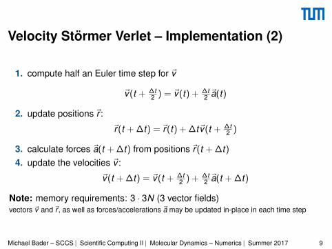
Velocity Stormer Verlet – Implementation (2)

1. compute half an Euler time step for ~v

~v(t + ∆t2 ) = ~v(t) + ∆t

2~a(t)

2. update positions ~r :

~r(t + ∆t) = ~r(t) + ∆t~v(t + ∆t2 )

3. calculate forces ~a(t + ∆t) from positions ~r(t + ∆t)4. update the velocities ~v :

~v(t + ∆t) = ~v(t + ∆t2 ) + ∆t

2~a(t + ∆t)

Note: memory requirements: 3 · 3N (3 vector fields)vectors ~v and~r , as well as forces/accelerations ~a may be updated in-place in each time step


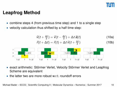
Leapfrog Method

• combine steps 4 (from previous time step) and 1 to a single step• velocity calculation thus shifted by a half time step:

~v(t + ∆t2 ) = ~v(t − ∆t

2 ) + ∆t ~a(t) (10a)~r(t + ∆t) = ~r(t) + ∆t ~v(t + ∆t

2 ) (10b)


r

v

F

t-Dt/2 t+Dt/2t-Dt/2 t+Dt/2 t-Dt/2 t+Dt/2 t-Dt/2 t+Dt/2

tt-Dt t+Dt

• exact arithmetic: Stormer Verlet, Velocity Stormer Verlet and LeapfrogScheme are equivalent

• the latter two are more robust w.r.t. roundoff errors


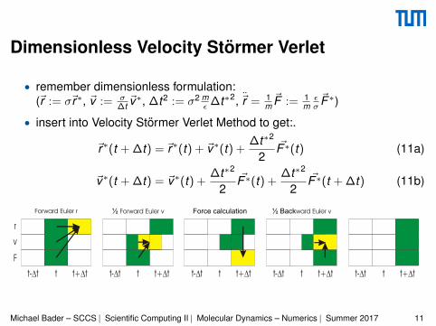
Dimensionless Velocity Stormer Verlet

• remember dimensionless formulation:(~r := σ~r∗, ~v := σ

∆t~v∗, ∆t2 := σ2 m

ε ∆t∗2, ~r = 1m~F := 1

mεσ~F ∗)

• insert into Velocity Stormer Verlet Method to get:.

~r∗(t + ∆t) = ~r∗(t) + ~v∗(t) +∆t∗2

2~F ∗(t) (11a)

~v∗(t + ∆t) = ~v∗(t) +∆t∗2

2~F ∗(t) +

∆t∗2

2~F ∗(t + ∆t) (11b)


r

v

F

tt-Dt t+Dttt-Dt t+Dt

Forward Euler r ½ Forward Euler v Force calculation ½ Backward Euler v


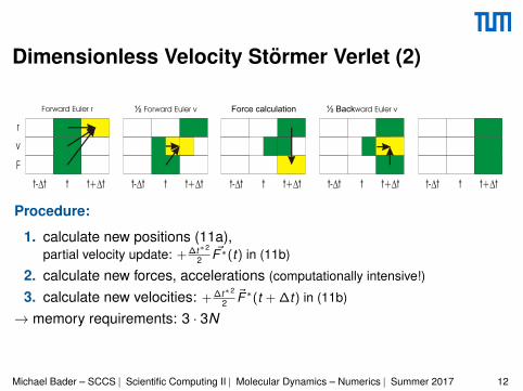
Dimensionless Velocity Stormer Verlet (2)


r

v

F

tt-Dt t+Dttt-Dt t+Dt

Forward Euler r ½ Forward Euler v Force calculation ½ Backward Euler v

Procedure:

1. calculate new positions (11a),partial velocity update: + ∆t∗2

2~F∗(t) in (11b)

2. calculate new forces, accelerations (computationally intensive!)

3. calculate new velocities: + ∆t∗2

2~F∗(t + ∆t) in (11b)

→ memory requirements: 3 · 3N


Outlook: Leapfrog Method with Thermostat

• Leapfrog method:

~v(t + ∆t2 ) = ~v(t − ∆t

2 ) + ∆t ~a(t)

~r(t + ∆t) = ~r(t) + ∆t ~v(t + ∆t2 )

t-Dt t+Dt t+Dt t-Dt t+Dt

r

v

F

tt-Dt t+Dt tt-Dt t+Dt tt-Dt t+Dt tt-Dt t+Dt tt-Dt t+Dt

Thermostat

• intermediate step may be introduced for the thermostat~v(t) := 1

2

(~v(t + ∆t

2 ) + ~v(t − ∆t2 ))

to synchronize velocity:

~vact (t) = ~v(t − ∆t2 ) + ∆t

2~a(t) (13a)

~v(t + ∆t2 ) = (2β − 1)~vact (t) + ∆t

2~a(t) (13b)


Evaluation of Time Integration Methods

• accuracy (not of great importance for exact particle positions)• stability• conservation→ of phase space density (symplectic)→ of energy→ of momentum

(especially with PBC→ Periodic Boundary Conditions)

• reversibility of time• use of resources:

– computational effort (number of force evaluations)– maximum time step size– memory usage


Reversibility of Time

• time reversal for a closed system means• a turnaround of the velocities and also momentums;

positions at the inversion point stay constant• traverse of a trajectory back in the direction of the origin

• demand for symmetry for time integration methods+ satisfied by Verlet method, e.g.− not satisfied by, e.g., Euler method, Predictor Corrector methods

(also not by standard Runge-Kutta methods)• contradiction with

• the H-theorem (increase of entropy, irreversible processes)?(Loschmidt’s paradox)

• the second theorem of thermodynamics?• reversibility in theory only for a very short time

• Lyapunov instability⇒ Kolmogorov entropy


Lyapunov Instability

• Basic question: how does a model behave with slightly disturbed initialcondition?

• Example of a simple system:• stable case:

jumping ball on a plane with slightly disturbed initial horizontalvelocity⇒ linear increase of the disturbance

• instable case:jumping ball on a sphere with slightly disturbed initial horizontalvelocity⇒ exponential increase of the disturbance (Lyapunovexponent)

• for the instable case, small disturbances result in large changes:chaotic behaviour (butterfly leading to a hurricane?)

• non-linear differential equations are often dynamically instable


Lyapunov Instability: A Numerical Experiment

• setup of 4000 fcc atoms• for a second setup, the position of a single

atom was displaced by 0.001• this atom is traced in both setups

colours indicate velocity

2.5 3

3.5 4

4.5 5

5.5 7.1 7.2

7.3 7.4

7.5 7.6

7.7

3.5

3.6

3.7

3.8

3.9 4

tracing a Molecule (with initial displacement)

Molecule 25, run1Molecule 25, run2

4.1


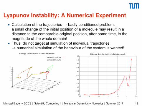
Lyapunov Instability: A Numerical Experiment• Calculation of the trajectories→ badly conditioned problem:

a small change of the initial position of a molecule may result in adistance to the comparable original position, after some time, in themagnitude of the whole domain!

• Thus: do not target at simulation of individual trajectories→ numerical simulation of the behaviour of the system is wanted!

2.5 3

3.5 4

4.5 5

5.5 7.1 7.2

7.3 7.4

7.5 7.6

7.7

3.5

3.6

3.7

3.8

3.9 4

tracing a Molecule (with initial displacement)

Molecule 25, run1Molecule 25, run2

4.1

0

0.05

0.1

0.15

0.2

0.25

0.3

0.35

0.4

0.45

0.5

2.5 3 3.5 4 4.5 5 5.5

Molecule deviation (with initial displacement)


molecular dynamics – numerics

Documents