package ‘snsequate’ - the comprehensive r archive … ‘snsequate’ september 10, 2017 type...
TRANSCRIPT

Package ‘SNSequate’September 10, 2017
Type Package
Title Standard and Nonstandard Statistical Models and Methods for TestEquating
Version 1.3.1
Depends R (>= 2.10), magic, stats
Imports methods, emdbook, plyr, progress, knitr, statmod
Description Contains functions to perform various models andmethods for test equating. It currently implements the traditionalmean, linear and equipercentile equating methods, as well as themean-mean, mean-sigma, Haebara and Stocking-Lord IRT linking methods.It also supports newest methods such that local equating, kernelequating (using Gaussian, logistic and uniform kernels) with presmoothing,and IRT parameter linking methods based on asymmetric item characteristicfunctions. Functions to obtain both standard error of equating (SEE)and standard error of equating difference between two equatingfunctions (SEED) are also implemented for the kernel method ofequating.
License GPL (>= 2)
URL http://www.mat.puc.cl/~jgonzale
Suggests testthat
NeedsCompilation no
Author Jorge Gonzalez Burgos [cre, aut],Daniel Leon Acuna [ctb]
Maintainer Jorge Gonzalez Burgos <[email protected]>
Repository CRAN
Date/Publication 2017-09-10 16:10:38 UTC
R topics documented:SNSequate-package . . . . . . . . . . . . . . . . . . . . . . . . . . . . . . . . . . . . . 2ACTmKB . . . . . . . . . . . . . . . . . . . . . . . . . . . . . . . . . . . . . . . . . . 3
1

2 SNSequate-package
bandwidth . . . . . . . . . . . . . . . . . . . . . . . . . . . . . . . . . . . . . . . . . . 4BNP.eq . . . . . . . . . . . . . . . . . . . . . . . . . . . . . . . . . . . . . . . . . . . 7BNP.eq.predict . . . . . . . . . . . . . . . . . . . . . . . . . . . . . . . . . . . . . . . 8CBdata . . . . . . . . . . . . . . . . . . . . . . . . . . . . . . . . . . . . . . . . . . . 9contaminate_sample . . . . . . . . . . . . . . . . . . . . . . . . . . . . . . . . . . . . 10eqp.eq . . . . . . . . . . . . . . . . . . . . . . . . . . . . . . . . . . . . . . . . . . . . 10gof . . . . . . . . . . . . . . . . . . . . . . . . . . . . . . . . . . . . . . . . . . . . . . 12irt.eq . . . . . . . . . . . . . . . . . . . . . . . . . . . . . . . . . . . . . . . . . . . . . 13irt.link . . . . . . . . . . . . . . . . . . . . . . . . . . . . . . . . . . . . . . . . . . . . 15KB36 . . . . . . . . . . . . . . . . . . . . . . . . . . . . . . . . . . . . . . . . . . . . 17KB36.1PL . . . . . . . . . . . . . . . . . . . . . . . . . . . . . . . . . . . . . . . . . . 18KB36_t . . . . . . . . . . . . . . . . . . . . . . . . . . . . . . . . . . . . . . . . . . . 19ker.eq . . . . . . . . . . . . . . . . . . . . . . . . . . . . . . . . . . . . . . . . . . . . 19le.eq . . . . . . . . . . . . . . . . . . . . . . . . . . . . . . . . . . . . . . . . . . . . . 23lin.eq . . . . . . . . . . . . . . . . . . . . . . . . . . . . . . . . . . . . . . . . . . . . 25loglin.smooth . . . . . . . . . . . . . . . . . . . . . . . . . . . . . . . . . . . . . . . . 27Math20EG . . . . . . . . . . . . . . . . . . . . . . . . . . . . . . . . . . . . . . . . . . 30Math20SG . . . . . . . . . . . . . . . . . . . . . . . . . . . . . . . . . . . . . . . . . . 30mea.eq . . . . . . . . . . . . . . . . . . . . . . . . . . . . . . . . . . . . . . . . . . . . 31pasted_table_to_df . . . . . . . . . . . . . . . . . . . . . . . . . . . . . . . . . . . . . 32PREp . . . . . . . . . . . . . . . . . . . . . . . . . . . . . . . . . . . . . . . . . . . . 33rowBlockSum . . . . . . . . . . . . . . . . . . . . . . . . . . . . . . . . . . . . . . . . 34SEED . . . . . . . . . . . . . . . . . . . . . . . . . . . . . . . . . . . . . . . . . . . . 35sim_unimodal . . . . . . . . . . . . . . . . . . . . . . . . . . . . . . . . . . . . . . . . 36
Index 38
SNSequate-package Standard and Nonstandard Statistical Models and Methods for TestEquating
Description
The package contains functions to perform various models and methods for test equating. It cur-rently implements the traditional mean, linear and equipercentile equating methods, as well as themean-mean, mean-sigma, Haebara and Stocking-Lord IRT linking methods. It also supports newestmethods such that local equating, kernel equating (using Gaussian, logistic and uniform kernels),and IRT parameterlinking methods based on asymmetric item characteristic functions. Functions toobtain both standard error of equating (SEE) and standard error of equating difference between twoequating functions (SEED) are also implmented for the kernel method of equating.
Details
Package: SNSequateType: PackageVersion: 1.1-1Date: 2014-08-08License: GPL (>= 2)

ACTmKB 3
Author(s)
Jorge Gonzalez Burgos
Maintainer: Jorge Gonzalez Burgos <[email protected]>
References
Estay, G. (2012). Characteristic Curves Scale Transformation Methods Using Asymmetric ICCs forIRT Equating. Unpublished MSc. Thesis. Pontificia Universidad Catolica de Chile.
Gonzalez, J. (2013). Statistical Models and Inference for the True Equating Transformation in theContext of Local Equating. Journal of Educational Measurement, 50(3), 315-320.
Gonzalez, J. (2014). SNSequate: Standard and Nonstandard Statistical Models and Methods forTest Equating. Journal of Statistical Software, 59(7), 1-30.
Holland, P. and Thayer, D. (1989). The kernel method of equating score distributions. (TechnicalReport No 89-84). Princeton, NJ: Educational Testing Service.
Holland, P., King, B. and Thayer, D. (1989). The standard error of equating for the kernel methodof equating score distributions (Tech. Rep. No. 89-83). Princeton, NJ: Educational Testing Service.
Kolen, M., and Brennan, R. (2004). Test Equating, Scaling and Linking. New York, NY: Springer-Verlag.
Lord, F. (1980). Applications of Item Response Theory to Practical Testing Problems. LawrenceErlbaum Associates, Hillsdale, NJ.
Lord, F. and Wingersky, M. (1984). Comparison of IRT True-Score and Equipercentile Observed-Score Equatings. Applied Psychological Measurement,8(4), 453–461.
van der Linden, W. (2011). Local Observed-Score Equating. In A. von Davier (Ed.) StatisticalModels for Test Equating, Scaling, and Linking. New York, NY: Springer-Verlag.
van der Linden, W. (2013). Some Conceptual Issues in Observed-Score Equating. Journal ofEducational Measurement, 50(3), 249-285.
Von Davier, A., Holland, P., and Thayer, D. (2004). The Kernel Method of Test Equating. NewYork, NY: Springer-Verlag.
ACTmKB Scores on two 40-items ACT mathematics test forms
Description
The data set contains raw sample frequencies of number-right scores for two multiple choice 40-items mathematics tests forms. Form X was administered to 4329 examinees and form Y to 4152examinees. This data has been described and analized by Kolen and Brennan (2004).
Usage
data(ACTmKB)

4 bandwidth
Format
A 41x2 matrix containing raw sample frequencies (raws) for two tests (columns).
Source
The data come with the distribution of the RAGE-RGEQUATE software which is freely available athttps://education.uiowa.edu/centers/center-advanced-studies-measurement-and-assessment/computer-programs
References
Kolen, M., and Brennan, R. (2004). Test Equating, Scaling and Linking. New York, NY: Springer-Verlag.
Examples
data(ACTmKB)## maybe str(ACTmKB) ; plot(ACTmKB) ...
bandwidth Automatic selection of the bandwidth parameter h
Description
This functions implements the minimization of the combined penalty function described by Hollandand Thayer (1989); Von Davier et al, (2004). It returns the optimal value of h for kernel continuiza-tion, according to the above mentioned criteria. Different types of kernels (others than the gaussian)are accepted.
Usage
bandwidth(scores, kert, degree, design, Kp = 1, scores2, degreeXA, degreeYA,J, K, L, wx, wy, w, ...)
Arguments
Note that depending on the specified equating design, not all arguments are nec-essary as detailed below.
scores If the "EG" design is specified, a vector containing the raw sample frequenciescoming from one group taking the test.If the "SG" design is specified, a matrix containing the (joint) bivariate samplefrequencies for X (raws) and Y (columns).If the "CB" design is specified, a two column matrix containing the observedscores of the sample taking test X first, followed by test Y . The scores2 argu-ment is then used for the scores of the sample taking test Y first followed by testX .

bandwidth 5
If either the "NEAT_CB" or "NEAT_PSE" design is selected, a two columnmatrix containing the observed scores on test X (first column) and the observedscores on the anchor test A (second column). The scores2 argument is thenused for the observed scores on test Y .
kert A character string giving the type of kernel to be used for continuization. Currentoptions include "gauss", "logis", and "uniform" for the gaussian, logistic anduniform kernels, respectively
degree Either a number or vector indicating the number of power moments to be fittedto the marginal distributions, or the number or cross moments to be fitted to thejoint distributions, respectively. For the "EG" design it will be a number (seeDetails).
design A character string indicating the equating design (one of "EG", "SG", "CB","NEAT_CE", "NEAT_PSE")
Kp A number which acts as a weight for the second term in the combined penaliza-tion function used to obtain h (see details).
scores2 Only used for the "CB", "NEAT_CE" and "NEAT_PSE" designs. See the de-scription of scores.
degreeXA A vector indicating the number of power moments to be fitted to the marginaldistributions X and A, and the number or cross moments to be fitted to the jointdistribution (X,A) (see details). Only used for the "NEAT_CE" and "NEAT_PSE"designs.
degreeYA Only used for the "NEAT_CE" and "NEAT_PSE" designs (see the descriptionfor degreeXA)
J The number of possible X scores. Only needed for "CB", "NEAT_CB" and"NEAT_PSE" designs
K The number of possible Y scores. Only needed for "CB", "NEAT_CB" and"NEAT_PSE" designs
L The number of possible A scores. Needed for "NEAT_CB" and "NEAT_PSE"designs
wx A number that satisfies 0 ≤ wX ≤ 1 indicating the weight put on the data thatis not subject to order effects. Only used for the "CB" design.
wy A number that satisfies 0 ≤ wY ≤ 1 indicating the weight put on the data thatis not subject to order effects. Only used for the "CB" design.
w A number that satisfies 0 ≤ w ≤ 1 indicating the weight given to population P .Only used for the "NEAT" design.
... Further arguments currently not used.
Details
To automatically select h, the function minimizes
PEN1(h) +K × PEN2(h)
where PEN1(h) =∑j(rj − fh(xj))
2, and PEN2(h) =∑j Aj(1 − Bj). The terms A and B
are such that PEN2 acts as a smoothness penalty term that avoids rapid fluctuations in the approxi-mated density (see Chapter 10 in Von Davier, 2011 for more details). TheK term corresponds to the

6 bandwidth
Kp argument of the bandwidth function. The r values are assumed to be estimated by polynomialloglinear models of specific degree, which come from a call to loglin.smooth.
Value
A number which is the optimal value of h.
Author(s)
Jorge Gonzalez B. <[email protected]>
References
Gonzalez, J. (2014). SNSequate: Standard and Nonstandard Statistical Models and Methods forTest Equating. Journal of Statistical Software, 59(7), 1-30.
Von Davier, A., Holland, P., and Thayer, D. (2004). The Kernel Method of Test Equating. NewYork, NY: Springer-Verlag.
A. von Davier (Ed.) (2011). Statistical Models for Equating, Scaling, and Linking. New York:Springer
See Also
loglin.smooth
Examples
#Example: The "Standard" column and firsts two rows of Table 10.1 in#Chapter 10 of Von Davier 2011
data(Math20EG)
hx.logis<-bandwidth(scores=Math20EG[,1],kert="logis",degree=2,design="EG")$hhx.unif<-bandwidth(scores=Math20EG[,1],kert="unif",degree=2,design="EG")$hhx.gauss<-bandwidth(scores=Math20EG[,1],kert="gauss",degree=2,design="EG")$h
hy.logis<-bandwidth(scores=Math20EG[,2],kert="logis",degree=3,design="EG")$hhy.unif<-bandwidth(scores=Math20EG[,2],kert="unif",degree=3,design="EG")$hhy.gauss<-bandwidth(scores=Math20EG[,2],kert="gauss",degree=3,design="EG")$h
partialTable10.1<-rbind(c(hx.logis,hx.unif,hx.gauss),c(hy.logis,hy.unif,hy.gauss))
dimnames(partialTable10.1)<-list(c("h.x","h.y"),c("Logistic","Uniform","Gaussian"))partialTable10.1

BNP.eq 7
BNP.eq Bayesian non-parametric model for test equating
Description
The Bayesian nonparametric (BNP) approach (Ghoshand Ramamoorthi, 2003; Hjort et al., 2010)starts by focusing on spaces of distribution functions, so that uncertainty is expressed on F itself.The prior distribution p(F) is defined on the space F of all distribution functions defined on X .If X is an infinite set then F is infinite-dimensional, and the corresponding prior model p(F) on Fis termed nonparametric. The prior probability model is also referred to as a random probabilitymeasure (RPM), and it essentially corresponds to a distribution on the space of all distributions onthe set X . Thus Bayesian nonparametric models are probability models defined on a function space(Muller and Quintana, 2004).
Gonzalez et al. (2015) proposed a Bayesian non-parametric approach for equating. The main ideaconsists of introducing covariate dependent BNP models for a collection of covariate-dependentequating transformations{ϕzf ,zt(·) : zf , zt ∈ L
}Usage
BNP.eq(scores_x, scores_y, range_scores = NULL, design = "EG",covariates = NULL, prior = NULL, mcmc = NULL, normalize = TRUE)
Arguments
scores_x Vector. Scores of form X.
scores_y Vector. Scores of form Y.
range_scores Vector of length 2. Represent the minimum and maximum scores in the test.
design Character. Only supports ’EG’ design now.
covariates Data.frame. A data frame with factors, containing covariates for test X and Y,stacked in that order.
prior List. Prior information for BNP model.
mcmc List. MCMC information for BNP model.
normalize Logical. Whether normalize or not the response variable. This is due to Berstein’spolynomials. Default is TRUE.
Details
Lorem ipsum dolor sit amet, consectetur adipiscing elit. Vivamus finibus vitae eros quis dictum.Donec lacus risus, facilisis quis tincidunt et, tincidunt sed mi. Nullam ullamcorper eros est, sedfringilla metus volutpat eu. Etiam ornare nulla id lorem posuere, eu vehicula urna vestibulum.Quisque luctus, diam ac mattis faucibus, leo felis tincidunt urna, eu tempus massa neque nec nibh.Aliquam erat volutpat. Fusce tempor mattis enim quis pretium. Aliquam volutpat luctus felis, necfringilla enim tincidunt sed. Nam nec leo quis erat lobortis vulputate ac at neque

8 BNP.eq.predict
Value
A ’BNP.eq’ object, which is list containing the following items:
Y Response variable.
X Design Matrix.
fit DPpackage object. Fitted model with raw samples.
max_score Maximum score of test.
patterns A matrix describing the different patterns formed from the factors in the covariables.
patterns_freq The normalized frequency of each pattern.
Author(s)
Daniel Leon A. <[email protected]>, Felipe Barrientos <[email protected]>.
References
asdasd
BNP.eq.predict Prediction step for Bayesian non-parametric model for test equating
Description
The
Usage
BNP.eq.predict(model, from = NULL, into = NULL, alpha = 0.05)
Arguments
model A ’BNP.eq’ object.
from Numeric. A vector of indices indicating from which patterns equating should beperformed. The covariates involved are integrated out.
into Numeric. A vector of indices indicating into which patterns equating should beperformed. The covariates involved are integrated out.
alpha Numeric. Significance for credible bands.
Details
Lorem ipsum dolor sit amet, consectetur adipiscing elit. Vivamus finibus vitae eros quis dictum.Donec lacus risus, facilisis quis tincidunt et, tincidunt sed mi. Nullam ullamcorper eros est, sedfringilla metus volutpat eu. Etiam ornare nulla id lorem posuere, eu vehicula urna vestibulum.Quisque luctus, diam ac mattis faucibus, leo felis tincidunt urna, eu tempus massa neque nec nibh.Aliquam erat volutpat. Fusce tempor mattis enim quis pretium. Aliquam volutpat luctus felis, necfringilla enim tincidunt sed. Nam nec leo quis erat lobortis vulputate ac at neque

CBdata 9
Value
A ’BNP.eq.predict’ object, which is list containing the following items:
pdf A list of PDF’s.
cdf A list of CDF’s.
equ Numeric. Equated values.
grid Numeric. Grid used to evaluate pdf’s and cdf’s.
Author(s)
Daniel Leon A. <[email protected]>, Felipe Barrientos <[email protected]>.
References
asdasd
CBdata Observed (raw) score values for two different tests
Description
The data set is from a small field study from an international testing program. It contains theobserved scores for two tests X (with 75 items) and Y (with 76 items) administered to two inde-pendent, random samples of examinees from a single population P . For more details, see Chapter9 in Von Davier et al, (2004) from where the data were obtained.
Usage
data(CBdata)
Format
A list with elements containing the observed scores of the sample taking test X first, followed bytest Y (datX1Y2), and the scores of the sample taking test Y first followed by test X (datX2Y1).
References
Von Davier, A., Holland, P., and Thayer, D. (2004). The Kernel Method of Test Equating. NewYork, NY: Springer-Verlag.
Examples
data(CBdata)## maybe str(CBdata) ; ...
10 eqp.eq
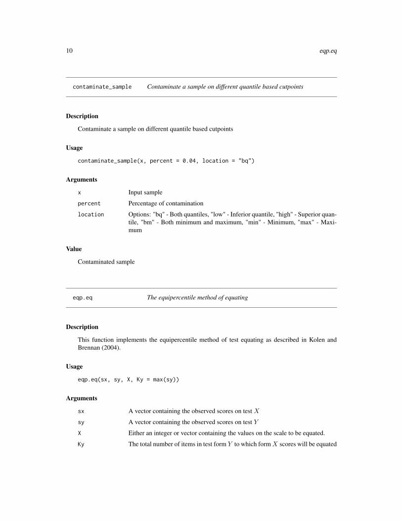
contaminate_sample Contaminate a sample on different quantile based cutpoints
Description
Contaminate a sample on different quantile based cutpoints
Usage
contaminate_sample(x, percent = 0.04, location = "bq")
Arguments
x Input sample
percent Percentage of contamination
location Options: "bq" - Both quantiles, "low" - Inferior quantile, "high" - Superior quan-tile, "bm" - Both minimum and maximum, "min" - Minimum, "max" - Maxi-mum
Value
Contaminated sample
eqp.eq The equipercentile method of equating
Description
This function implements the equipercentile method of test equating as described in Kolen andBrennan (2004).
Usage
eqp.eq(sx, sy, X, Ky = max(sy))
Arguments
sx A vector containing the observed scores on test X
sy A vector containing the observed scores on test Y
X Either an integer or vector containing the values on the scale to be equated.
Ky The total number of items in test form Y to which formX scores will be equated

eqp.eq 11
Details
The function implements the equipercentile method of equating as described in Kolen and Brennan(2004). Given observed scores sx and sy, the functions calculates
ϕ(x) = G−1(F (x))
where F and G are the cdf of scores on test forms X and Y , respectively.
Value
A two column matrix with the values of ϕ() (second column) for each scale value x (first column)
Author(s)
Jorge Gonzalez B. <[email protected]>
References
Gonzalez, J. (2014). SNSequate: Standard and Nonstandard Statistical Models and Methods forTest Equating. Journal of Statistical Software, 59(7), 1-30.
Kolen, M., and Brennan, R. (2004). Test Equating, Scaling and Linking. New York, NY: Springer-Verlag.
See Also
mea.eq, lin.eq, ker.eq
Examples
### Example from Kolen and Brennan (2004), pages 41-42:### (scores distributions have been transformed to vectors of scores)
sx<-c(0,0,1,1,1,2,2,3,3,4)sy<-c(0,1,1,2,2,3,3,3,4,4)x<-2eqp.eq(sx,sy,2)
# Whole scale range (Table 2.3 in KB)eqp.eq(sx,sy,0:4)

12 gof
gof Functions to assess model fitting.
Description
This function contains various measures to assess the model’s goodness of fit.
Usage
gof(obs, fit, methods=c("FT"), p.out=FALSE)
Arguments
obs A vector containing the observed values.
fit A vector containing the fitted values.
methods A character vector containing one or many of the following methods:
"FT" Freeman-Tukey Residuals. This is the default test."Chisq" Pearson’s Chi-squared test."KL" Symmetrised Kullback-Leibler divergence [1].
p.out Boolean. Decides whether or not to display plots (on corresponding methods).
Author(s)
Daniel Leon A. <[email protected]>
References
Gonzalez, J. (2014). SNSequate: Standard and Nonstandard Statistical Models and Methods forTest Equating. Journal of Statistical Software, 59(7), 1-30.
Kolen, M., and Brennan, R. (2004). Test Equating, Scaling and Linking. New York, NY: Springer-Verlag.
[1] https://en.wikipedia.org/wiki/Kullback-Leibler_divergence
Examples
data(Math20EG)mod <- ker.eq(scores=Math20EG,kert="gauss",degree=c(2,3),design="EG")
gof(Math20EG[,1], mod$rj*mod$nx, method=c("FT", "KL"))

irt.eq 13
irt.eq IRT methods for Test Equating
Description
Implements methods to perform Test Equating over IRT models.
Usage
irt.eq(n_items, param_x, param_y, theta_points=NULL, weights=NULL,n_points=10, w=1, A=NULL, B=NULL, link=NULL,method_link=NULL, common=NULL, method="TS", D=1.7,...)
Arguments
n_items Number of items of the test
param_x Estimated parameters for IRT model on test X. This list must have the followingstructure: list(a, b, c), where each parameter is a vector with the respectiveestimate for each subject. If you want to perform other models (i.e. Rasch),replace according with a vector of zeros.
param_y Estimated parameters for IRT model on test Y. This list must have the followingstructure: list(a, b, c), where each parameter is a vector with the respectiveestimate for each subject. If you want to perform other models (i.e. Rasch),replace according with a vector of zeros.
method A string, either "TS" or "OS". Each one stands for "True Score Equating" and"Observed score equating". Notice that OS requires the additional arguments"theta_points" and "weigths".
theta_points For "OS" only. Points over a grid of possible values of θ to integrate out theability term.
weights For "OS" only. Weigths for integrate out the ability term. If is NULL, themethod assumes the distribution of ability is characterized by a finite number ofabilities (Kolen and Brennan 2013, pg 199).
n_points In case theta_ponints is not provided, is the length of the grid for the gaussianquadrature.
A, B Scaling parameters. In the case they are not provided, they will be calculateddepending on the next described inputs.
link An irt.link object.
method_link Method used to estimate A and B. Default is "mean/sigma". Others are "mean/mean","Haebara" and "Stocklord". For more information see irt.link
common Common items to estimate A and B. Default asume all items are common.
w Weight factor between real and synthetic population.
D Scaling parameter. Default is 1.7
... Further arguments.

14 irt.eq
Details
This function implements two methods to perform Test Equating over Item Response Theory mod-els (Kolen and Brennan 2013).
"True Score Equating" relate number-correct scores on Form X and Form Y. Assumes that the truescore associated with each θ is equivalent to the true score on another form associated with that θ.
"Observed Score Equating" uses the IRT model to produce an estimated distribution of observednumber-correct scores on each form. Using the compound binomial distribution (Lord and Winger-sky 1984) to find the conditional distributions f(x|θ), and then integrate out the θ parameter. After-wards, an Equipercentile Equating process is done over the estimated distributions.
Value
An object of the clas irt.eq is returned. Depending on the method used, the outputs are:
True Score Equating A list(n_items, theta_equivalent, tau_y) containing the number of items, thetheta equivalent values on Form X to Form Y and the equivalent scores.
Observed Score Equating A list(n_items, f_hat, g_hat, e_Y_x) containing the number of items,the estimated distributions and the equated values.
Author(s)
Daniel Leon A. <[email protected]>
References
Kolen, M. J., & Brennan, R. L. (2013). Test Equating, Scaling, and Linking: Methods and Practices,Third Edition. Springer Science & Business Media.
See Also
irt.link
Examples
data(KB36_t)dfo <- KB36_t
param_x <- list(a=dfo[,3],b=dfo[,4],c=dfo[,5])param_y <- list(a=dfo[,7],b=dfo[,8],c=dfo[,9])
theta_points=c(-5.2086,-4.163,-3.1175,-2.072,-1.0269,0.0184,1.0635,2.109,3.1546,4.2001)
weights=c(0.000101,0.00276,0.03021,0.142,0.3149,0.3158,0.1542,0.03596,0.003925,0.000186)
irt.eq(36, param_x, param_y, method="TS", A=1, B=0)irt.eq(36, param_x, param_y, theta_points, weights, method="OS",
A=1, B=0)

irt.link 15
irt.link IRT parameter linking methods
Description
The function implements parameter linking methods to transform IRT scales. Mean-mean, mean-sigma, Haebara, and Stocking and Lord methods are available (see details).
Usage
irt.link(parm, common, model, icc, D, ...)
Arguments
parm A 6 column matrix containing item parameter estimates from an IRT model. Thefirst three columns contains the parameters for the form Y fit, and the last threethose of form X. The order for item paramters in the matrix is discrimination,difficulty, and guessing. See details.
common A vector indicating the position where common items are located
model A character string indicating the underlying IRT model: "1PL", "2PL", "3PL".
icc A character string indicating the type of icc used in the characteristic curvemethods (see details). Available options are "logistic" and "cloglog".
D A number indicating the value of the constant D (see details)
... Further arguments currently not used.
Details
The function implments various methods of IRT parameter linking (a.k.a, scale transformationmethods). It calculates the linking constants A and B to tranform parameter estimates. When assum-ing a 1PL model, the matrix parm should contain a column of ones and a column of zeroes in theplaces where discrimination and guessing parameters are located, respectively.
The characteristic curve methods (Haebara and Stocking and Lord) rely on the item characteristiccurve pijassumed for the probability of a correct answer
pij = P (Yij = 1 | θi) = cj + (1− cj)exp[Daj(θi − βj)]
1 + exp[Daj(θi − βj)]
Besides the traditional logistic model, the irt.link() function allows the use of an asymetriccloglog ICC. See the help for KB36.1PL data set, where some details on how to fit a 1PL modelwith cloglog link in lmer are given.
For more details on characteristic curve methods see Kolen and Brennan (2004).
Value
A list with the constants A and B calculated using the four different methods

16 irt.link
Note
Currently, the cloglog ICC is only implmented for the 1PL model. A 1PL model with asymetriccloglog link can be fitted in R using the lmer() function in package lme4
Author(s)
Jorge Gonzalez B. <[email protected]>
References
Gonzalez, J. (2014). SNSequate: Standard and Nonstandard Statistical Models and Methods forTest Equating. Journal of Statistical Software, 59(7), 1-30.
Kolen, M., and Brennan, R. (2004). Test Equating, Scaling and Linking. New York, NY: Springer-Verlag.
Estay, G. (2012). Characteristic Curves Scale Transformation Methods Using Asymmetric ICCs forIRT Equating. Unpublished MSc. Thesis. Pontificia Universidad Catolica de Chile
See Also
mea.eq, lin.eq, ker.eq
Examples
#### Example. KB, Table 6.6data(KB36)parm.x = KB36$KBformX_parparm.y = KB36$KBformY_parcomitems = seq(3,36,3)parm = as.data.frame(cbind(parm.y, parm.x))
# Table 6.6 KBirt.link(parm,comitems,model="3PL",icc="logistic",D=1.7)
# Same data but assuming a 1PL model. The parameter estimates are load from# the KB36.1PL data set. See the help for KB36.1PL data for details on how these# estimates were obtained using \code{lmer()} (see also Table 6.13 in KB)
data(KB36.1PL)
#preparing the input data matrices for irt.link() functionb.log.y<-KB36.1PL$b.logistic[,2]b.log.x<-KB36.1PL$b.logistic[,1]b.clog.y<-KB36.1PL$b.cloglog[,2]b.clog.x<-KB36.1PL$b.cloglog[,1]
parm2 = as.data.frame(cbind(1,b.log.y,0, 1,b.log.x, 0))parm3 = as.data.frame(cbind(1,b.clog.y,0, 1,b.clog.x,0))
#vector indicating common items

KB36 17
comitems = seq(3,36,3)
#Calculating the B constant under the logistic-link modelirt.link(parm2,comitems,model="1PL",icc="logistic",D=1.7)
#Calculating the B constant under the cloglog-link modelirt.link(parm3,comitems,model="1PL",icc="cloglog",D=1.7)
KB36 Data on two 36-items test forms
Description
The data set contains both response patterns and item parameters estimates following a 3PL modelfor two 36-items tests forms. Form X was administered to 1655 examinees and form Y to 1638examinees. Also, 12 out of the 36 items are common between both test forms (items 3, 6, 9, 12,15, 18, 21, 24, 27, 30, 33, 36). This data has been described and analized by Kolen and Brennan(2004).
Usage
data(KB36)
Format
A list with four elements containing binary data matrices of responses (KBformX and KBformY) andthe corresponding parameter estimates which result from a 3PL fit to both data matrices (KBformX_parand KBformY_par).
Source
The data come with the distribution of the CIPE software which is freely available at https://education.uiowa.edu/centers/center-advanced-studies-measurement-and-assessment/computer-programs. The list of item parameters estimates can be found in Table 6.5 of Kolen andBrennan (2004).
References
Kolen, M., and Brennan, R. (2004). Test Equating, Scaling and Linking. New York, NY: Springer-Verlag.
Examples
data(KB36)## maybe str(KB36) ; plot(KB36) ...

18 KB36.1PL
KB36.1PL Difficulty parameter estimates for KB36 data under a 1PL model
Description
This data set contains the estimated item difficuty parameters for the KB36 data, assuming a 1PLmodel. Two sets of parameters estimates for test forms X and Y are available: one that resultsfrom a fit assuming the traditional logistic link, and one which comes from the fit using a cloglog(asymmetric) link.
Usage
data(KB36.1PL)
Format
A list of 2 elements containing item (difficulty) parameters estimates for test forms X and Y underthe logistic-link model (b.logistic), and under the cloglog-link model (b.cloglog)
Details
This data set is used to illustrate the characteristic curve methods (Haebara and Stocking-Lord)which can use an asymmetric cloglog ICC for the calculations, as described in Estay (2012).
A 1PL model using both logistic and cloglog link can be fitted using the lmer() function in thelme4 R package (see De Boeck et. al, 2011 for details).
Source
The item parameter estimates for the 1PL model with logistic link are also shown in Table 6.13 ofKolen and Brennan (2004).
References
De Boeck, P., Bakker, M., Zwitser, R., Nivard, M., Hofman, A.,Tuerlinckx, F., Partchev, I. (2011).The Estimation of Item Response Models with the lmer Function from the lme4 Package in R.Journal of Statistical Software, 39(12), 1-28.
Kolen, M., and Brennan, R. (2004). Test Equating, Scaling and Linking. New York, NY: Springer-Verlag.
Estay, G. (2012). Characteristic Curves Scale Transformation Methods Using Asymmetric ICCs forIRT Equating. Unpublished MSc. Thesis. Pontificia Universidad Catolica de Chile
Examples
data(KB36.1PL)## maybe str(KB36.1PL) ; plot(KB36.1PL) ...

KB36_t 19
KB36_t Data on two 36-items test forms
Description
The data set contains item parameters estimates following a 3PL model for two 36-items tests forms,rescaled using mean-sigma method’s A and B using all common items except item 27. This datahas been described and analized by Kolen and Brennan (2004), Table 6.8.
Usage
data(KB36_t)
Format
A dataframe where each column represent item parameter estimates of forms X and Y, with theirrespective p-values.
References
Kolen, M., and Brennan, R. (2004). Test Equating, Scaling and Linking. New York, NY: Springer-Verlag.
See Also
KB36
Examples
data(KB36_t)
ker.eq The Kernel method of test equating
Description
This function implements the kernel method of test equating as described in Holland and Thayer(1989), and Von Davier et al. (2004). Nonstandard kernels others than the gaussian are available.Associated standard error of equating are also provided.
Usage
ker.eq(scores, kert, hx=NULL, hy=NULL, degree, design, Kp=1, scores2,degreeXA, degreeYA, J, K, L, wx, wy, w,gapsX=NULL, gapsY=NULL, gapsA=NULL, lumpX=NULL, lumpY=NULL, lumpA=NULL,alpha=NULL, h.adap=NULL)

20 ker.eq
Arguments
Note that depending on the specified equating design, not all arguments are nec-essary as detailed below.
scores If the "EG" design is specified, a two column matrix containing the raw samplefrequencies coming from the two groups of scores to be equated. It is assumedthat the data in the first and second columns come from tests X and Y , respec-tively.If the "SG" design is specified, a matrix containing the (joint) bivariate samplefrequencies for X (raws) and Y (columns).If the "CB" design is specified, a two column matrix containing the observedscores of the sample taking test X first, followed by test Y . The scores2 argu-ment is then used for the scores of the sample taking test Y first followed by testX .If either the "NEAT_CB" or "NEAT_PSE" design is selected, a two columnmatrix containing the observed scores on test X (first column) and the observedscores on the anchor test A (second column). The scores2 argument is thenused for the observed scores on test Y .
kert A character string giving the type of kernel to be used for continuization. Cur-rent options include "gauss", "logis", "uniform", "epan" and "adap" for thegaussian, logistic, uniform, Epanechnikov and Adaptative kernels, respectively
hx An integer indicating the value of the bandwidth parameter to be used for kernelcontinuization of F (x). If not provided (Default), this value is automaticallycalculated (see details).
hy An integer indicating the value of the bandwidth parameter to be used for kernelcontinuization of G(y). If not provided (Default), this value is automaticallycalculated (see details).
degree A vector indicating the number of power moments to be fitted to the marginaldistributions ("EG" design), and/or the number or cross moments to be fitted tothe joint distributions (see Details).
design A character string indicating the equating design (one of "EG", "SG", "CB","NEAT_CE", "NEAT_PSE")
Kp A number which acts as a weight for the second term in the combined penaliza-tion function used to obtain h (see details).
scores2 Only used for the "CB", "NEAT_CE" and "NEAT_PSE" designs. See the de-scription of scores.
degreeXA A vector indicating the number of power moments to be fitted to the marginaldistributions X and A, and the number or cross moments to be fitted to the jointdistribution (X,A) (see details). Only used for the "NEAT_CE" and "NEAT_PSE"designs.
degreeYA Only used for the "NEAT_CE" and "NEAT_PSE" designs (see the descriptionfor degreeXA)
J The number of possible X scores. Only needed for "CB", "NEAT_CB" and"NEAT_PSE" designs

ker.eq 21
K The number of possible Y scores. Only needed for "CB", "NEAT_CB" and"NEAT_PSE" designs
L The number of possible A scores. Needed for "NEAT_CB" and "NEAT_PSE"designs
wx A number that satisfies 0 ≤ wX ≤ 1 indicating the weight put on the data thatis not subject to order effects. Only used for the "CB" design.
wy A number that satisfies 0 ≤ wY ≤ 1 indicating the weight put on the data thatis not subject to order effects. Only used for the "CB" design.
w A number that satisfies 0 ≤ w ≤ 1 indicating the weight given to population P .Only used for the "NEAT" design.
gapsX A list object containing:
index A vector of indices between 0 and J to smooth "gaps", usually ocur-ring at regular intervals due to scores rounded to integer values and othermethodological factors.
degree An integer indicating the maximum degree of the moments fitted by thelog-linear model.
Only used for the "NEAT" design.
gapsY A list object containing:
index A vector of indices between 0 and K.degree An integer indicating the maximum degree of the moments fitted.
Only used for the "NEAT" design.
gapsA A list object containing:
index A vector of indices between 0 and L.degree An integer indicating the maximum degree of the moments fitted.
Only used for the "NEAT" design.
lumpX An integer to represent the index where an artificial "lump" is created in themarginal distribution of frecuencies for X due to recording of negative roundedformulas or any other methodological artifact.
lumpY An integer to represent the index where an artificial "lump" is created in themarginal distribution of frecuencies for Y .
lumpA An integer to represent the index where an artificial "lump" is created in themarginal distribution of frecuencies for A.
alpha Only for Adaptative Kernel. Sensitivity parameter.
h.adap Only for Adaptative Kernel. A list(hx, hy) containing bandwidths for Adaptativekernel for each Form.
... Further arguments currently not used.
Details
This is a generic function that implements the kernel method of test equating as described in VonDavier et al. (2004). Given test scores X and Y , the functions calculates
eY (x) = G−1hY(FhX
(x; r), s)

22 ker.eq
where r and s are estimated score probabilities obtained via loglinear smoothing (see loglin.smooth).The value of hX and hY can either be specified by the user or left unspecified (default) in whichcase they are automatically calculated. For instance, one can specifies large values of hX and hY ,so that the eY (x) tends to the linear equating function (see Theorem 4.5 in Von Davier et al, 2004for more details).
Value
An object of class ker.eq representing the kernel equating process. Generic functions such asprint, and summary have methods to show the results of the equating. The results include summarystatistics, equated values, standard errors of equating, and others.
The function SEED can be used to obtain standard error of equating differences (SEED) of twoobjects of class ker.eq. The function PREp can be used on a ker.eq object to obtain the percentagerelative error measure (see Von Davier et al, 2004).
Scores The possible values of xj and ykeqYx The equated values of test X in test Y scale
eqXy The equated values of test Y in test X scale
SEEYx The standard error of equating for equating X to Y
SEEXy The standard error of equating for equating Y to X
Author(s)
Jorge Gonzalez B. <[email protected]>
References
Gonzalez, J. (2014). SNSequate: Standard and Nonstandard Statistical Models and Methods forTest Equating. Journal of Statistical Software, 59(7), 1-30.
Holland, P. and Thayer, D. (1989). The kernel method of equating score distributions. (TechnicalReport No 89-84). Princeton, NJ: Educational Testing Service.
Holland, P., King, B. and Thayer, D. (1989). The standard error of equating for the kernel methodof equating score distributions (Tech. Rep. No. 89-83). Princeton, NJ: Educational Testing Service.
Von Davier, A., Holland, P., and Thayer, D. (2004). The Kernel Method of Test Equating. NewYork, NY: Springer-Verlag.
See Also
loglin.smooth, SEED, PREp
Examples
#Kernel equating under the "EG" designdata(Math20EG)mod<-ker.eq(scores=Math20EG,kert="gauss",hx=NULL,hy=NULL,degree=c(2,3),design="EG")
summary(mod)

le.eq 23
#Reproducing Table 7.6 in Von Davier et al, (2004)
scores<-0:20SEEXy<-mod$SEEXySEEYx<-mod$SEEYx
Table7.6<-cbind(scores,SEEXy,SEEYx)Table7.6
#Other nonstandard kernels. Table 10.3 in Von Davier (2011).
mod.logis<-ker.eq(scores=Math20EG,kert="logis",hx=NULL,hy=NULL,degree=c(2,3),design="EG")mod.unif<-ker.eq(scores=Math20EG,kert="unif",hx=NULL,hy=NULL,degree=c(2,3),design="EG")mod.gauss<-ker.eq(scores=Math20EG,kert="gauss",hx=NULL,hy=NULL,degree=c(2,3),design="EG")
XtoY<-cbind(mod.logis$eqYx,mod.unif$eqYx,mod.gauss$eqYx)YtoX<-cbind(mod.logis$eqXy,mod.unif$eqXy,mod.gauss$eqXy)
Table10.3<-cbind(XtoY,YtoX)Table10.3
## Examples using Adaptive and Epanechnikov kernelsx_sim = c(1,2,3,4,5,6,7,8,9,10,11,10,9,8,7,6,5,4,3,2,1)prob_sim = x_sim/sum(x_sim)set.seed(1)sim = rmultinom(1, p = prob_sim, size = 1000)
x_asimD = c(1,7,13,18,22,24,25,24,20,18,16,15,13,9,5,3,2.5,1.5,1.5,1,1)probas_asimD = x_asimD/sum(x_asimD)set.seed(1)asim = rmultinom(1, p = probas_asimD, size = 1000)
scores = cbind(asim,sim)
mod.adap = ker.eq(scores,degree=c(2,2),design="EG",kert="adap")mod.epan = ker.eq(scores,degree=c(2,2),design="EG",kert="epan")
le.eq Local equating methods
Description
This function implements the local method of equating as descibed in van der Linden (2011).
Usage
le.eq(S.X, It.X, It.Y, Theta)

24 le.eq
Arguments
S.X A vector containing the observed scores of the sample taking test X .
It.X A matrix of item parameter estimates coming from an IRT model for test formX(difficulty, discrimation and guessing parameters are located in the first, secondand third column, respectively).
It.Y A matrix of item parameter estimates coming from an IRT model for test formY .
Theta Either a number or vector of values representing the value of theta where tocondition on (see details)
Details
The function implements the local equating method as described in van der Linden (2011). Basedon Lord (1980) principle of equity, local equating methods utilizes the conditional on abilities dis-tributions of scores to obtain the transformation ϕ. The method leads to a family of transformationsof the form
ϕ(x; θ) = G−1Y |θ(FX|θ(x)), θ ∈ R
The conditional distributions of X and Y are obtained using the algorithm described by Lord andWingersky (1984). Among other possibilities, a value for θ can be a EAP, ML or MAP estimationof it, for and underlying IRT model (for example, using the ltm R package (Rizopoulos, 2006)).
Value
A list containing the observed scores to be equated, the corresponding ability estimates where tocondition on, and the equated values
Author(s)
Jorge Gonzalez B. <[email protected]>
References
Gonzalez, J. (2014). SNSequate: Standard and Nonstandard Statistical Models and Methods forTest Equating. Journal of Statistical Software, 59(7), 1-30.
Lord, F. (1980). Applications of Item Response Theory to Practical Testing Problems. LawrenceErlbaum Associates, Hillsdale, NJ.
Lord, F. and Wingersky, M. (1984). Comparison of IRT True-Score and Equipercentile Observed-Score Equatings. Applied Psychological Measurement,8(4), 453–461.
Rizopoulos, D. (2006). ltm: An R package for latent variable modeling and item response theoryanalyses. Journal of Statistical Software, 17(5), 1–25.
van der Linden, W. (2011). Local Observed-Score Equating. In A. von Davier (Ed.) StatisticalModels for Test Equating, Scaling, and Linking. New York, NY: Springer-Verlag.
See Also
mea.eq, eqp.eq, lin.eq ker.eq

lin.eq 25
Examples
## Artificial data for two 5-items tests forms. Both forms are assumed## being fitted by a 3PL model.
## Create (artificial) item parameters matrices for test form X and Yai<-c(1,0.8,1.2,1.1,0.9)bi<-c(-2,-1,0,1,2)ci<-c(0.1,0.15,0.05,0.1,0.2)itx<-rbind(bi,ai,ci)ai<-c(0.5,1.4,1.2,0.8,1)bi<-c(-1,-0.5,1,1.5,0)ci<-c(0.1,0.2,0.1,0.15,0.1)ity<-rbind(bi,ai,ci)
#Two individuals with different ability (1 and 2) obtain the same score 2.#Their corresponding equated scores values are:le.eq(c(2,2),itx,ity,c(1,2))
lin.eq The linear method of equating
Description
This function implements the linear method of test equating as described in Kolen and Brennan(2004).
Usage
lin.eq(sx, sy, scale)
Arguments
sx A vector containing the observed scores of the sample taking test X .
sy A vector containing the observed scores of the sample taking test Y .
scale Either an integer or vector containing the values on the scale to be equated.
Details
The function implements the linear method of equating as described in Kolen and Brennan (2004).Given observed scores sx and sy, the functions calculates
ϕ(x;µx, µy, σx, σy) =σxσy
(x− µx) + µy
where µx, µy, σx, σy are the score means and standard deviations on test X and Y , respectively.

26 lin.eq
Value
A two column matrix with the values of ϕ() (second column) for each scale value x (first column)
Author(s)
Jorge Gonzalez B. <[email protected]>
References
Gonzalez, J. (2014). SNSequate: Standard and Nonstandard Statistical Models and Methods forTest Equating. Journal of Statistical Software, 59(7), 1-30.
Kolen, M., and Brennan, R. (2004). Test Equating, Scaling and Linking. New York, NY: Springer-Verlag.
See Also
mea.eq, eqp.eq, ker.eq
Examples
#Artificial data for two two 100 item tests forms and 5 individuals in each groupx1<-c(67,70,77,79,65,74)y1<-c(77,75,73,89,68,80)
#Score means and sdmean(x1); mean(y1)sd(x1); sd(y1)
#An equivalent form y1 score of 72 on form x1lin.eq(x1,y1,72)
#Equivalent form y1 score for the whole scale rangelin.eq(x1,y1,0:100)
#A plot comparing mean, linear and identity equatingplot(0:100,0:100, type='l', xlim=c(-20,100),ylim=c(0,100),lwd=2.0,lty=1,ylab="Form Y raw score",xlab="Form X raw score")abline(a=5,b=1,lwd=2,lty=2)abline(a=mean(y1)-(sd(y1)/sd(x1))*mean(x1),b=sd(y1)/sd(x1),,lwd=2,lty=3)arrows(72, 0, 72, 77,length = 0.15,code=2,angle=20)arrows(72, 77, -20, 77,length = 0.15,code=2,angle=20)abline(v=0,lty=2)legend("bottomright",lty=c(1,2,3), c("Identity","Mean","Linear"),lwd=c(2,2,2))

loglin.smooth 27
loglin.smooth Pre-smoothing using log-linear models.
Description
This function fits log-linear models to score data and provides estimates of the (vector of) scoreprobabilities as well as the C matrix decomposition of their covariance matrix, according to thespecified equating design (see Details).
Usage
loglin.smooth(scores, degree, design, scores2, degreeXA, degreeYA,J, K, L, wx, wy, w, gapsX, gapsY, gapsA, lumpX, lumpY, lumpA, ...)
Arguments
Note that depending on the specified equating design, not all arguments are nec-essary as detailed below.
scores If the "EG" design is specified, a vector containing the raw sample frequenciescoming from one group taking the test.If the "SG" design is specified, a matrix containing the (joint) bivariate samplefrequencies for X (raws) and Y (columns).If the "CB" design is specified, a two column matrix containing the observedscores of the sample taking test X first, followed by test Y . The scores2 argu-ment is then used for the scores of the sample taking test Y first followed by testX .If either the "NEAT_CB" or "NEAT_PSE" design is selected, a two columnmatrix containing the observed scores on test X (first column) and the observedscores on the anchor test A (second column). The scores2 argument is thenused for the observed scores on test Y .
degree Either a number or vector indicating the number of power moments to be fittedto the marginal distributions, or the number or cross moments to be fitted to thejoint distributions, respectively. For the "EG" design it will be a number (seeDetails).
design A character string indicating the equating design (one of "EG", "SG", "CB","NEAT_CE", "NEAT_PSE")
scores2 Only used for the "CB", "NEAT_CE" and "NEAT_PSE" designs. See the de-scription of scores.
degreeXA A vector indicating the number of power moments to be fitted to the marginaldistributions X and A, and the number or cross moments to be fitted to the jointdistribution (X,A) (see details). Only used for the "NEAT_CE" and "NEAT_PSE"designs.
degreeYA Only used for the "NEAT_CE" and "NEAT_PSE" designs (see the descriptionfor degreeXA)
28 loglin.smooth
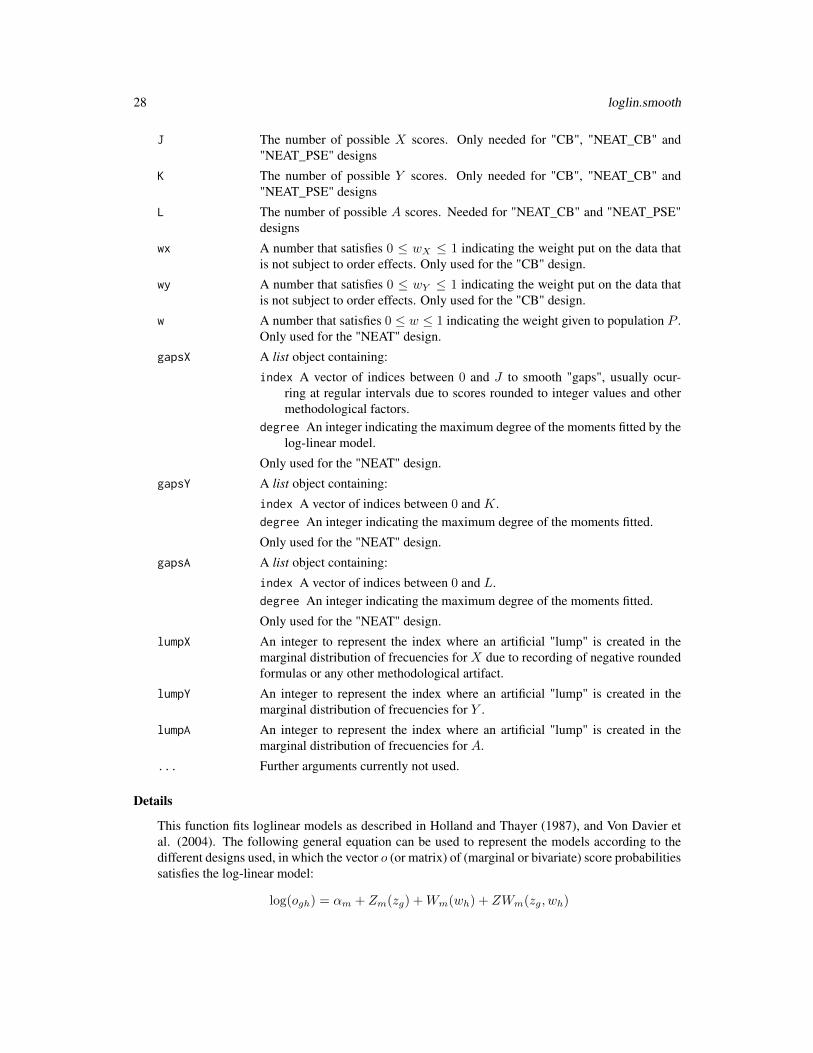
J The number of possible X scores. Only needed for "CB", "NEAT_CB" and"NEAT_PSE" designs
K The number of possible Y scores. Only needed for "CB", "NEAT_CB" and"NEAT_PSE" designs
L The number of possible A scores. Needed for "NEAT_CB" and "NEAT_PSE"designs
wx A number that satisfies 0 ≤ wX ≤ 1 indicating the weight put on the data thatis not subject to order effects. Only used for the "CB" design.
wy A number that satisfies 0 ≤ wY ≤ 1 indicating the weight put on the data thatis not subject to order effects. Only used for the "CB" design.
w A number that satisfies 0 ≤ w ≤ 1 indicating the weight given to population P .Only used for the "NEAT" design.
gapsX A list object containing:
index A vector of indices between 0 and J to smooth "gaps", usually ocur-ring at regular intervals due to scores rounded to integer values and othermethodological factors.
degree An integer indicating the maximum degree of the moments fitted by thelog-linear model.
Only used for the "NEAT" design.
gapsY A list object containing:
index A vector of indices between 0 and K.degree An integer indicating the maximum degree of the moments fitted.
Only used for the "NEAT" design.
gapsA A list object containing:
index A vector of indices between 0 and L.degree An integer indicating the maximum degree of the moments fitted.
Only used for the "NEAT" design.
lumpX An integer to represent the index where an artificial "lump" is created in themarginal distribution of frecuencies for X due to recording of negative roundedformulas or any other methodological artifact.
lumpY An integer to represent the index where an artificial "lump" is created in themarginal distribution of frecuencies for Y .
lumpA An integer to represent the index where an artificial "lump" is created in themarginal distribution of frecuencies for A.
... Further arguments currently not used.
Details
This function fits loglinear models as described in Holland and Thayer (1987), and Von Davier etal. (2004). The following general equation can be used to represent the models according to thedifferent designs used, in which the vector o (or matrix) of (marginal or bivariate) score probabilitiessatisfies the log-linear model:
log(ogh) = αm + Zm(zg) +Wm(wh) + ZWm(zg, wh)

loglin.smooth 29
where Zm(zg) =∑TZm
i=1 βzmi(zg)i, Wm(wh) =
∑TWm
i=1 βWmi(wh)i, and, ZWm(zg, wh) =∑IZm
i=1
∑IWm
i′=1 βZWmii′(zg)i(wh)i
′.
The symbols will vary according to the different equating designs specified. Possible values are:o = p(12), p(21), p, q; Z = X,Y ; W = Y,A; z = x, y; w = y, a; m = (12), (21), P,Q; g = j, k;h = l, k.
Particular cases of this general equation for each of the equating designs can be found in Von Davieret al (2004) (e.g., Equations (7.1) and (7.2) for the "EG" design, Equation (8.1) for the "SG" design,Equations (9,1) and (9.2) for the "CB" design).
Value
sp.est The estimated score probabilities
C The C matrix which is so that Σ = CCt
Author(s)
Jorge Gonzalez B. <[email protected]>
References
Gonzalez, J. (2014). SNSequate: Standard and Nonstandard Statistical Models and Methods forTest Equating. Journal of Statistical Software, 59(7), 1-30.
Holland, P. and Thayer, D. (1987). Notes on the use of loglinear models for fitting discrete proba-bility distributions. Research Report 87-31, Princeton NJ: Educational Testing Service.
Von Davier, A., Holland, P., and Thayer, D. (2004). The Kernel Method of Test Equating. NewYork, NY: Springer-Verlag.
[1] Moses, T. "Paper SA06_05 Using PROC GENMOD for Loglinear Smoothing Tim Moses andAlina A. von Davier, Educational Testing Service, Princeton, NJ".
See Also
glm, ker.eq
Examples
#Table 7.4 from Von Davier et al. (2004)data(Math20EG)rj<-loglin.smooth(scores=Math20EG[,1],degree=2,design="EG")$sp.estsk<-loglin.smooth(scores=Math20EG[,2],degree=3,design="EG")$sp.estscore<-0:20Table7.4<-cbind(score,rj,sk)Table7.4
## Example taken from [1]score <- 0:20freq <- c(10, 2, 5, 8, 7, 9, 8, 7, 8, 5, 5, 4, 3, 0, 2, 0, 1, 0, 2, 1, 0)ldata <- data.frame(score, freq)
plot(ldata, pch=16, main="Data w Lump at 0")

30 Math20SG
m1 = loglin.smooth(scores=ldata$freq,kert="gauss",degree=c(3),design="EG")m2 = loglin.smooth(scores=ldata$freq,kert="gauss",degree=c(3),design="EG",lumpX=0)Ns = sum(ldata$freq)points(m1$sp.est*Ns, col=2, pch=16)points(m2$sp.est*Ns, col=3, pch=16) # Preserves the lump
Math20EG Scores on two 20-items mathematics tests.
Description
The data set contains raw sample frequencies of number-right scores for two parallel 20-itemsmathematics tests given to two samples from a national population of examinees. This data hasbeen described and analized by Holland and Thayer (1989); Von Davier et al, (2004) (see also VonDavier, 2011 where other applications using these data set are shown).
Usage
data(Math20EG)
Format
A 21x2 matrix containing raw sample frequencies (raws) for two parallel tests (columns)
References
Holland, P. and Thayer, D. (1989). The kernel method of equating score distributions. (TechnicalReport No 89-84). Princeton, NJ: Educational Testing Service.
Von Davier, A., Holland, P., and Thayer, D. (2004). The Kernel Method of Test Equating. NewYork, NY: Springer-Verlag.
Examples
data(Math20EG)## maybe str(Math20EG) ; ...
Math20SG Bivariate score frequencies on two 20-items mathematics tests.
Description
The data set contains the bivariate sample frequencies of number-right scores for two parallel 20-items mathematics tests given to a sample from a national population of examinees. This data hasbeen described and analized by Holland and Thayer (1989); Von Davier et al, (2004).

mea.eq 31
Usage
data(Math20SG)
Format
A 21x21 matrix containing the bivariate sample frequencies for X (raws) and Y (columns)
References
Holland, P. and Thayer, D. (1989). The kernel method of equating score distributions. (TechnicalReport No 89-84). Princeton, NJ: Educational Testing Service.
Von Davier, A., Holland, P., and Thayer, D. (2004). The Kernel Method of Test Equating. NewYork, NY: Springer-Verlag.
Examples
data(Math20SG)## maybe str(Math20SG) ; ...
mea.eq The mean method of equating
Description
This function implements the mean method of test equating as described in Kolen and Brennan(2004).
Usage
mea.eq(sx, sy, scale)
Arguments
sx A vector containing the observed scores of the sample taking test X .
sy A vector containing the observed scores of the sample taking test Y .
scale Either an integer or vector containing the values on the scale to be equated.
Details
The function implements the mean method of equating as described in Kolen and Brennan (2004).Given observed scores sx and sy, the functions calculates
ϕ(x;µx, µy) = x− µx + µy
where µx and µy are the score means on test X and Y , respectively.

32 pasted_table_to_df
Value
A two column matrix with the values of ϕ() (second column) for each scale value x (first column)
Author(s)
Jorge Gonzalez B. <[email protected]>
References
Gonzalez, J. (2014). SNSequate: Standard and Nonstandard Statistical Models and Methods forTest Equating. Journal of Statistical Software, 59(7), 1-30.
Kolen, M., and Brennan, R. (2004). Test Equating, Scaling and Linking. New York, NY: Springer-Verlag.
See Also
lin.eq, eqp.eq, ker.eq, le.eq
Examples
#Artificial data for two two 100 item tests forms and 5 individuals in each groupx1<-c(67,70,77,79,65,74)y1<-c(77,75,73,89,68,80)
#Score meansmean(x1); mean(y1)
#An equivalent form y1 score of 72 on form x1mea.eq(x1,y1,72)
#Equivalent form y1 score for the whole scale rangemea.eq(x1,y1,0:100)
pasted_table_to_df Transform a table from String to Data Frame.
Description
The usual way to compare results is using tables from books. This method accept as input a pastedString, usually copied from a LaTeX table, and create a Data Frame. Assumes the input is separatedevenly by a character, default is an empty space.
Usage
pasted_table_to_df(string, n_cols, sep = " ", header = TRUE)
PREp 33
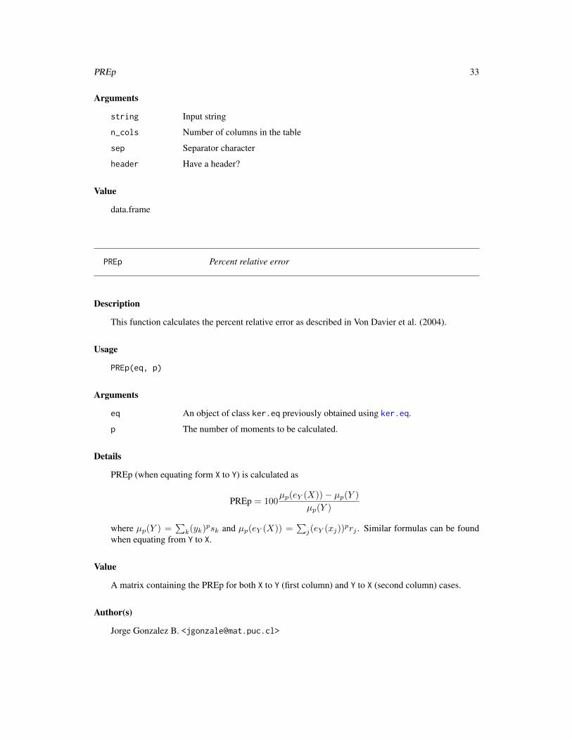
Arguments
string Input string
n_cols Number of columns in the table
sep Separator character
header Have a header?
Value
data.frame
PREp Percent relative error
Description
This function calculates the percent relative error as described in Von Davier et al. (2004).
Usage
PREp(eq, p)
Arguments
eq An object of class ker.eq previously obtained using ker.eq.
p The number of moments to be calculated.
Details
PREp (when equating form X to Y) is calculated as
PREp = 100µp(eY (X))− µp(Y )
µp(Y )
where µp(Y ) =∑k(yk)psk and µp(eY (X)) =
∑j(eY (xj))
prj . Similar formulas can be foundwhen equating from Y to X.
Value
A matrix containing the PREp for both X to Y (first column) and Y to X (second column) cases.
Author(s)
Jorge Gonzalez B. <[email protected]>

34 rowBlockSum
References
Gonzalez, J. (2014). SNSequate: Standard and Nonstandard Statistical Models and Methods forTest Equating. Journal of Statistical Software, 59(7), 1-30.
Von Davier, A., Holland, P., and Thayer, D. (2004). The Kernel Method of Test Equating. NewYork, NY: Springer-Verlag.
See Also
ker.eq
Examples
#Example: Table 7.5 in Von Davier et al. (2004)
data(Math20EG)mod.gauss<-ker.eq(scores=Math20EG,kert="gauss", hx = NULL, hy = NULL,degree=c(2, 3),design="EG")PREp(mod.gauss,10)
rowBlockSum Take a matrix and sum blocks of rows
Description
The original data set contains very long column headers. This function does a keyword search overthe headers to find those column headers that match a particular keyword, e.g., mean, median, etc.
Usage
rowBlockSum(mat, blocksize, w = NULL)
Arguments
mat Input matrix
blocksize Size of the row blocks
w (Optional) Vector for weighted sum
Value
Matrix

SEED 35
SEED Standard error of equating difference
Description
This function calculates the standard error of equating diference (SEED) as described in Von Davieret al. (2004).
Usage
SEED(eq1, eq2, ...)
Arguments
eq1 An object of class ker.eq which contains one of the two estimated equatedfunctions to be used for the SEED.
eq2 An object of class ker.eq which contains one of the two estimated equatedfunctions to be used for the SEED.
... Further arguments currently not in use
Details
The SEED can be used as a measure to choose whether to support or not a certain equating functionon another another one. For instance, when hX and hY tends to infinity, then the (gaussian kernel)eY (x) equating function tends to the linear equating function (see Theorem 4.5 in Von Davier et al,2004 for more details). Thus, one can calculate the measure
SEEDY (x) =
√V ar(eY (x)− LinY (x))
to decide between eY (x) and LinY (x).
Value
A two column matrix with the values of SEEYx for each x in the first column and the values of SEEXyfor each y in the second column
Author(s)
Jorge Gonzalez B. <[email protected]>
References
Gonzalez, J. (2014). SNSequate: Standard and Nonstandard Statistical Models and Methods forTest Equating. Journal of Statistical Software, 59(7), 1-30.
Von Davier, A., Holland, P., and Thayer, D. (2004). The Kernel Method of Test Equating. NewYork, NY: Springer-Verlag.

36 sim_unimodal
See Also
ker.eq
Examples
#Example: Figure7.7 in Von Davier et al, (2004)data(Math20EG)
mod.gauss<-ker.eq(scores=Math20EG,kert="gauss", hx = NULL, hy = NULL,degree=c(2, 3),design="EG")mod.linear<-ker.eq(scores=Math20EG,kert="gauss", hx = 20, hy = 20,degree=c(2, 3),design="EG")
Rx<-mod.gauss$eqYx-mod.linear$eqYxseed<-SEED(mod.gauss,mod.linear)$SEEDYx
plot(0:20,Rx,ylim=c(-0.8,0.8),pch=15)abline(h=0)points(0:20,2*seed,pch=0)points(0:20,-2*seed,pch=0)
#Example Figure 10.4 in Von Davier (2011)mod.unif<-ker.eq(scores=Math20EG,kert="unif", hx = NULL, hy = NULL,degree=c(2, 3),design="EG")mod.logis<-ker.eq(scores=Math20EG,kert="logis", hx = NULL, hy = NULL,degree=c(2, 3),design="EG")
Rx1<-mod.logis$eqYx-mod.gauss$eqYxRx2<-mod.unif$eqYx-mod.gauss$eqYx
seed1<-SEED(mod.logis,mod.gauss)$SEEDYxseed2<-SEED(mod.unif,mod.gauss)$SEEDYx
plot(0:20,Rx1,ylim=c(-0.2,0.2),pch=15,main="LK vs GK",ylab="",xlab="Scores")abline(h=0)points(0:20,2*seed1,pch=0)points(0:20,-2*seed1,pch=0)
plot(0:20,Rx2,ylim=c(-0.2,0.2),pch=15,main="UK vs GK",ylab="",xlab="Scores")abline(h=0)points(0:20,2*seed2,pch=0)points(0:20,-2*seed2,pch=0)
sim_unimodal Simulate different unimodal distributions.
Description
Simulate different unimodal, skewed distributions based on different mean and variance parameters.
Usage
sim_unimodal(n, x_mean, x_var, N_item, seed = NULL, name = NULL)

sim_unimodal 37
Arguments
n Size of the simulated distribution
x_mean Mean
x_var Variance
N_item Number of items simulated
seed (Optional) Set a random seed
name (Optional) Sample based on the names given by Keats & Lord (1962). Optionsare: "GANA", "MACAA", "TQS8", "WM8", "WMI".
Details
All the inner working of this procedure can be seen in Keats & Lord (1962).
Value
Simulated values

Index
∗Topic BNPBNP.eq, 7BNP.eq.predict, 8
∗Topic BayesianBNP.eq, 7BNP.eq.predict, 8
∗Topic IRT parameter linkingirt.link, 15
∗Topic Traditional equating methodseqp.eq, 10gof, 12lin.eq, 25mea.eq, 31
∗Topic datasetsACTmKB, 3CBdata, 9KB36, 17KB36.1PL, 18KB36_t, 19Math20EG, 30Math20SG, 30
∗Topic equating,BNP.eq, 7BNP.eq.predict, 8
∗Topic equatingBNP.eq, 7BNP.eq.predict, 8
∗Topic kernel equatingbandwidth, 4irt.eq, 13ker.eq, 19PREp, 33SEED, 35
∗Topic local equatingle.eq, 23
∗Topic non-parametrics,BNP.eq, 7BNP.eq.predict, 8
∗Topic package
SNSequate-package, 2∗Topic smoothing
loglin.smooth, 27
ACTmKB, 3
bandwidth, 4BNP.eq, 7BNP.eq.predict, 8
CBdata, 9contaminate_sample, 10
eqp.eq, 10, 24, 26, 32
glm, 29gof, 12
irt.eq, 13irt.link, 13, 14, 15
KB36, 17KB36.1PL, 18KB36_t, 19ker.eq, 11, 16, 19, 24, 26, 29, 32–34, 36
le.eq, 23, 32lin.eq, 11, 16, 24, 25, 32loglin.smooth, 6, 22, 27
Math20EG, 30Math20SG, 30mea.eq, 11, 16, 24, 26, 31
pasted_table_to_df, 32PREp, 22, 33
rowBlockSum, 34
SEED, 22, 35sim_unimodal, 36SNSequate (SNSequate-package), 2SNSequate-package, 2
38