package ‘tolerance’ · tolerance-package 3 tolerance-package statistical tolerance intervals...

Package ‘tolerance’February 4, 2017

Type Package

Title Statistical Tolerance Intervals and Regions

Version 1.3.0

Date 2017-02-03

Depends R (>= 3.2.0)

Imports rgl, stats4

Description Statistical tolerance limits provide the limits between which we can expect to find a speci-fied proportion of a sampled population with a given level of confidence. This package pro-vides functions for estimating tolerance limits (intervals) for various univariate distributions (bi-nomial, Cauchy, discrete Pareto, exponential, two-parameter exponential, extreme value, hyper-geometric, Laplace, logistic, negative binomial, negative hypergeometric, normal, Pareto, Pois-son-Lindley, Poisson, uniform, and Zipf-Mandelbrot), Bayesian normal tolerance limits, multi-variate normal tolerance regions, nonparametric tolerance intervals, tolerance bands for regres-sion settings (linear regression, nonlinear regression, nonparametric regression, and multivari-ate regression), and analysis of variance tolerance intervals. Visualizations are also avail-able for most of these settings.

License GPL (>= 2)

NeedsCompilation no

Author Derek S. Young [aut, cre]

Maintainer Derek S. Young <[email protected]>

Repository CRAN

Date/Publication 2017-02-04 08:40:19

R topics documented:tolerance-package . . . . . . . . . . . . . . . . . . . . . . . . . . . . . . . . . . . . . . 3acc.samp . . . . . . . . . . . . . . . . . . . . . . . . . . . . . . . . . . . . . . . . . . . 4anovatol.int . . . . . . . . . . . . . . . . . . . . . . . . . . . . . . . . . . . . . . . . . 5bayesnormtol.int . . . . . . . . . . . . . . . . . . . . . . . . . . . . . . . . . . . . . . 7bintol.int . . . . . . . . . . . . . . . . . . . . . . . . . . . . . . . . . . . . . . . . . . . 9bonftol.int . . . . . . . . . . . . . . . . . . . . . . . . . . . . . . . . . . . . . . . . . . 12cautol.int . . . . . . . . . . . . . . . . . . . . . . . . . . . . . . . . . . . . . . . . . . 13

1

2 R topics documented:

diffnormtol.int . . . . . . . . . . . . . . . . . . . . . . . . . . . . . . . . . . . . . . . . 14DiffProp . . . . . . . . . . . . . . . . . . . . . . . . . . . . . . . . . . . . . . . . . . . 16DiscretePareto . . . . . . . . . . . . . . . . . . . . . . . . . . . . . . . . . . . . . . . . 18distfree.est . . . . . . . . . . . . . . . . . . . . . . . . . . . . . . . . . . . . . . . . . . 19dpareto.ll . . . . . . . . . . . . . . . . . . . . . . . . . . . . . . . . . . . . . . . . . . 20dparetotol.int . . . . . . . . . . . . . . . . . . . . . . . . . . . . . . . . . . . . . . . . 21exp2tol.int . . . . . . . . . . . . . . . . . . . . . . . . . . . . . . . . . . . . . . . . . . 23exptol.int . . . . . . . . . . . . . . . . . . . . . . . . . . . . . . . . . . . . . . . . . . 25exttol.int . . . . . . . . . . . . . . . . . . . . . . . . . . . . . . . . . . . . . . . . . . . 26F1 . . . . . . . . . . . . . . . . . . . . . . . . . . . . . . . . . . . . . . . . . . . . . . 28fidbintol.int . . . . . . . . . . . . . . . . . . . . . . . . . . . . . . . . . . . . . . . . . 29fidnegbintol.int . . . . . . . . . . . . . . . . . . . . . . . . . . . . . . . . . . . . . . . 31fidpoistol.int . . . . . . . . . . . . . . . . . . . . . . . . . . . . . . . . . . . . . . . . . 33gamtol.int . . . . . . . . . . . . . . . . . . . . . . . . . . . . . . . . . . . . . . . . . . 35hypertol.int . . . . . . . . . . . . . . . . . . . . . . . . . . . . . . . . . . . . . . . . . 37K.factor . . . . . . . . . . . . . . . . . . . . . . . . . . . . . . . . . . . . . . . . . . . 38K.factor.sim . . . . . . . . . . . . . . . . . . . . . . . . . . . . . . . . . . . . . . . . . 40K.table . . . . . . . . . . . . . . . . . . . . . . . . . . . . . . . . . . . . . . . . . . . . 42laptol.int . . . . . . . . . . . . . . . . . . . . . . . . . . . . . . . . . . . . . . . . . . . 44logistol.int . . . . . . . . . . . . . . . . . . . . . . . . . . . . . . . . . . . . . . . . . . 45mvregtol.region . . . . . . . . . . . . . . . . . . . . . . . . . . . . . . . . . . . . . . . 47mvtol.region . . . . . . . . . . . . . . . . . . . . . . . . . . . . . . . . . . . . . . . . . 48negbintol.int . . . . . . . . . . . . . . . . . . . . . . . . . . . . . . . . . . . . . . . . . 50NegHypergeometric . . . . . . . . . . . . . . . . . . . . . . . . . . . . . . . . . . . . . 52neghypertol.int . . . . . . . . . . . . . . . . . . . . . . . . . . . . . . . . . . . . . . . 54nlregtol.int . . . . . . . . . . . . . . . . . . . . . . . . . . . . . . . . . . . . . . . . . . 55norm.OC . . . . . . . . . . . . . . . . . . . . . . . . . . . . . . . . . . . . . . . . . . 57norm.ss . . . . . . . . . . . . . . . . . . . . . . . . . . . . . . . . . . . . . . . . . . . 59normtol.int . . . . . . . . . . . . . . . . . . . . . . . . . . . . . . . . . . . . . . . . . 61np.order . . . . . . . . . . . . . . . . . . . . . . . . . . . . . . . . . . . . . . . . . . . 63npregtol.int . . . . . . . . . . . . . . . . . . . . . . . . . . . . . . . . . . . . . . . . . 64nptol.int . . . . . . . . . . . . . . . . . . . . . . . . . . . . . . . . . . . . . . . . . . . 66paretotol.int . . . . . . . . . . . . . . . . . . . . . . . . . . . . . . . . . . . . . . . . . 68plottol . . . . . . . . . . . . . . . . . . . . . . . . . . . . . . . . . . . . . . . . . . . . 69poislind.ll . . . . . . . . . . . . . . . . . . . . . . . . . . . . . . . . . . . . . . . . . . 71poislindtol.int . . . . . . . . . . . . . . . . . . . . . . . . . . . . . . . . . . . . . . . . 72PoissonLindley . . . . . . . . . . . . . . . . . . . . . . . . . . . . . . . . . . . . . . . 74poistol.int . . . . . . . . . . . . . . . . . . . . . . . . . . . . . . . . . . . . . . . . . . 75regtol.int . . . . . . . . . . . . . . . . . . . . . . . . . . . . . . . . . . . . . . . . . . . 77simnormtol.int . . . . . . . . . . . . . . . . . . . . . . . . . . . . . . . . . . . . . . . . 79TwoParExponential . . . . . . . . . . . . . . . . . . . . . . . . . . . . . . . . . . . . . 81umatol.int . . . . . . . . . . . . . . . . . . . . . . . . . . . . . . . . . . . . . . . . . . 82uniftol.int . . . . . . . . . . . . . . . . . . . . . . . . . . . . . . . . . . . . . . . . . . 83ZipfMandelbrot . . . . . . . . . . . . . . . . . . . . . . . . . . . . . . . . . . . . . . . 85zipftol.int . . . . . . . . . . . . . . . . . . . . . . . . . . . . . . . . . . . . . . . . . . 87zm.ll . . . . . . . . . . . . . . . . . . . . . . . . . . . . . . . . . . . . . . . . . . . . . 89

Index 92

tolerance-package 3

tolerance-package Statistical Tolerance Intervals and Regions

Description

Statistical tolerance limits provide the limits between which we can expect to find a specified pro-portion of a sampled population with a given level of confidence. This package provides functionsfor estimating tolerance limits (intervals) for various univariate distributions (binomial, Cauchy,discrete Pareto, exponential, two-parameter exponential, extreme value, hypergeometric, Laplace,logistic, negative binomial, negative hypergeometric, normal, Pareto, Poisson-Lindley, Poisson,uniform, and Zipf-Mandelbrot), Bayesian normal tolerance limits, multivariate normal toleranceregions, nonparametric tolerance intervals, tolerance bands for regression settings (linear regres-sion, nonlinear regression, nonparametric regression, and multivariate regression), and analysis ofvariance tolerance intervals. Visualizations are also available for most of these settings.

Details

Package: toleranceType: PackageVersion: 1.3.0Date: 2017-02-03Imports: rgl, stats4License: GPL (>= 2)

Author(s)

Derek S. Young, Ph.D.

Maintainer: Derek S. Young <[email protected]>

References

Hahn, G. J. and Meeker, W. Q. (1991), Statistical Intervals: A Guide for Practitioners, Wiley-Interscience.

Krishnamoorthy, K. and Mathew, T. (2009), Statistical Tolerance Regions: Theory, Applications,and Computation, Wiley.

Patel, J. K. (1986), Tolerance Intervals - A Review, Communications in Statistics - Theory andMethodology, 15, 2719–2762.

Young, D. S. (2010), tolerance: An R Package for Estimating Tolerance Intervals, Journal ofStatistical Software, 36(5), 1–39.

Young, D. S. (2014), Computing Tolerance Intervals and Regions in R. In M. B. Rao and C. R.Rao (eds.), Handbook of Statistics, Volume 32: Computational Statistics with R, 309–338. North-Holland, Amsterdam.

4 acc.samp

See Also

confint

acc.samp Acceptance Sampling

Description

Provides an upper bound on the number of acceptable rejects or nonconformities in a process. Thisis similar to a 1-sided upper tolerance bound for a hypergeometric random variable.

Usage

acc.samp(n, N, alpha = 0.05, P = 0.99, AQL = 0.01, RQL = 0.02)

Arguments

n The sample size to be drawn from the inventory.

N The total inventory (or lot) size.

alpha 1-alpha is the confidence level for bounding the probability of accepting theinventory.

P The proportion of items in the inventory which are to be accountable.

AQL The acceptable quality level, which is the largest proportion of defects in a pro-cess considered acceptable. Note that 0 < AQL < 1.

RQL The rejectable quality level, which is the largest proportion of defects in anindependent lot that one is willing to tolerate. Note that AQL < RQL < 1.

Value

acc.samp returns a matrix with the following quantities:

acceptance.limit

The number of items in the sample which may be unaccountable, yet still beable to attain the desired confidence level 1-alpha.

lot.size The total inventory (or lot) size N.

confidence The confidence level 1-alpha.

P The proportion of accountable items specified by the user.

AQL The acceptable quality level as specified by the user. If the sampling were to berepeated numerous times as a process, then this quantity specifies the proportionof missing items considered acceptable from the process as a whole. Condition-ing on the calculated value for acceptance.limit, the AQL is used to estimatethe producer’s risk (see prod.risk below).

anovatol.int 5

RQL The rejectable quality level as specified by the user. This is the proportion ofindividual items in a sample one is willing to tolerate missing. Conditioningon the calculated value for acceptance.limit, the RQL is used to estimate theconsumer’s risk (see cons.risk below).

sample.size The sample size drawn as specified by n.

prod.risk The producer’s risk at the specified AQL. This is the probability of rejecting anaudit of a good inventory (also called the Type I error). A good inventory can berejected if an unfortunate random sample is selected (e.g., most of the missingitems happened to be selected for the audit). 1-prod.risk gives the confidencelevel of this sampling plan for the specified AQL and RQL. If it is lower thanthe confidence level desired (e.g., because the AQL is too high), then a warningmessage will be displayed.

cons.risk The consumer’s risk at the specified RQL. This is the probability of acceptingan audit of a bad inventory (also called the Type II error). A bad inventory canbe accepted if a fortunate random sample is selected (e.g., most of the missingitems happened to not be selected for the audit).

References

Montgomery, D. C. (2005), Introduction to Statistical Quality Control, Fifth Edition, John Wiley &Sons, Inc.

See Also

Hypergeometric

Examples

## A 90%/90% acceptance sampling plan for a sample of 450## drawn from a lot size of 960.

acc.samp(n = 450, N = 960, alpha = 0.10, P = 0.90, AQL = 0.07,RQL = 0.10)

anovatol.int Tolerance Intervals for ANOVA

Description

Tolerance intervals for each factor level in a balanced (or nearly-balanced) ANOVA.

Usage

anovatol.int(lm.out, data, alpha = 0.05, P = 0.99, side = 1,method = c("HE", "HE2", "WBE", "ELL", "KM","EXACT", "OCT"), m = 50)

6 anovatol.int

Arguments

lm.out An object of class lm (i.e., the results from the linear model fitting routine suchthat the anova function can act upon).

data A data frame consisting of the data fitted in lm.out. Note that data must haveone column for each main effect (i.e., factor) that is analyzed in lm.out and thatthese columns must be of class factor.

alpha The level chosen such that 1-alpha is the confidence level.

P The proportion of the population to be covered by this tolerance interval.

side Whether a 1-sided or 2-sided tolerance interval is required (determined by side = 1or side = 2, respectively).

method The method for calculating the k-factors. The k-factor for the 1-sided toler-ance intervals is performed exactly and thus is the same for the chosen method."HE" is the Howe method and is often viewed as being extremely accurate, evenfor small sample sizes. "HE2" is a second method due to Howe, which per-forms similarly to the Weissberg-Beatty method, but is computationally sim-pler. "WBE" is the Weissberg-Beatty method (also called the Wald-Wolfowitzmethod), which performs similarly to the first Howe method for larger samplesizes. "ELL" is the Ellison correction to the Weissberg-Beatty method when f isappreciably larger than n^2. A warning message is displayed if f is not largerthan n^2. "KM" is the Krishnamoorthy-Mathew approximation to the exact solu-tion, which works well for larger sample sizes. "EXACT" computes the k-factorexactly by finding the integral solution to the problem via the integrate func-tion. Note the computation time of this method is largely determined by m."OCT" is the Owen approach to compute the k-factor when controlling the tailsso that there is not more than (1-P)/2 of the data in each tail of the distribution.

m The maximum number of subintervals to be used in the integrate function.This is necessary only for method = "EXACT" and method = "OCT". The largerthe number, the more accurate the solution. Too low of a value can result in an er-ror. A large value can also cause the function to be slow for method = "EXACT".

Value

anovatol.int returns a list where each element is a data frame corresponding to each main effect(i.e., factor) tested in the ANOVA and the rows of each data frame are the levels of that factor. Thecolumns of each data frame report the following:

mean The mean for that factor level.

n The effective sample size for that factor level.

k The k-factor for constructing the respective factor level’s tolerance interval.

1-sided.lower The 1-sided lower tolerance bound. This is given only if side = 1.

1-sided.upper The 1-sided upper tolerance bound. This is given only if side = 1.



bayesnormtol.int 7

References

Howe, W. G. (1969), Two-Sided Tolerance Limits for Normal Populations - Some Improvements,Journal of the American Statistical Association, 64, 610–620.

Weissberg, A. and Beatty, G. (1969), Tables of Tolerance Limit Factors for Normal Distributions,Technometrics, 2, 483–500.

See Also

K.factor, normtol.int, lm, anova

Examples

## 90%/95% 2-sided tolerance intervals for a 2-way ANOVA## using the "warpbreaks" data.

attach(warpbreaks)

lm.out <- lm(breaks ~ wool + tension)out <- anovatol.int(lm.out, data = warpbreaks, alpha = 0.10,

P = 0.95, side = 2, method = "HE")out

plottol(out, x = warpbreaks)

bayesnormtol.int Bayesian Normal Tolerance Intervals

Description

Provides 1-sided or 2-sided Bayesian tolerance intervals under the conjugate prior for data dis-tributed according to a normal distribution.

Usage

bayesnormtol.int(x = NULL, norm.stats = list(x.bar = NA,s = NA, n = NA), alpha = 0.05, P = 0.99,side = 1, method = c("HE", "HE2", "WBE","ELL", "KM", "EXACT", "OCT"), m = 50,hyper.par = list(mu.0 = NULL,sig2.0 = NULL, m.0 = NULL, n.0 = NULL))

Arguments

x A vector of data which is distributed according to a normal distribution.

norm.stats An optional list of statistics that can be provided in-lieu of the full dataset. Ifprovided, the user must specify all three components: the sample mean (x.bar),the sample standard deviation (s), and the sample size (n).

8 bayesnormtol.int






hyper.par A list consisting of the hyperparameters for the conjugate prior: the hyperpa-rameters for the mean (mu.0 and n.0) and the hyperparameters for the variance(sig2.0 and m.0).

Details

Note that if one considers the non-informative prior distribution, then the Bayesian tolerance inter-vals are the same as the classical solution, which can be obtained by using normtol.int.

Value

bayesnormtol.int returns a data frame with items:

alpha The specified significance level.

P The proportion of the population covered by this tolerance interval.

x.bar The sample mean.

1-sided.lower The 1-sided lower Bayesian tolerance bound. This is given only if side = 1.

1-sided.upper The 1-sided upper Bayesian tolerance bound. This is given only if side = 1.

2-sided.lower The 2-sided lower Bayesian tolerance bound. This is given only if side = 2.

2-sided.upper The 2-sided upper Bayesian tolerance bound. This is given only if side = 2.

bintol.int 9

References

Aitchison, J. (1964), Bayesian Tolerance Regions, Journal of the Royal Statistical Society, SeriesB, 26, 161–175.

Guttman, I. (1970), Statistical Tolerance Regions: Classical and Bayesian, Charles Griffin andCompany.

Young, D. S., Gordon, C. M., Zhu, S., and Olin, B. D. (2016), Sample Size Determination Strategiesfor Normal Tolerance Intervals Using Historical Data, Quality Engineering (to appear).

See Also

Normal, normtol.int, K.factor

Examples

## 95%/85% 1-sided Bayesian normal tolerance limits for## a sample of size 100.

set.seed(100)x <- rnorm(100)out <- bayesnormtol.int(x = x, alpha = 0.05, P = 0.85,

side = 1, method = "EXACT",hyper.par = list(mu.0 = 0,sig2.0 = 1, n.0 = 10, m.0 = 10))

out

plottol(out, x, plot.type = "both", side = "upper",x.lab = "Normal Data")

bintol.int Binomial Tolerance Intervals

Description

Provides 1-sided or 2-sided tolerance intervals for binomial random variables. From a statisticalquality control perspective, these limits use the proportion of defective (or acceptable) items in asample to bound the number of defective (or acceptable) items in future productions of a specifiedquantity.

Usage

bintol.int(x, n, m = NULL, alpha = 0.05, P = 0.99, side = 1,method = c("LS", "WS", "AC", "JF", "CP", "AS","LO", "PR", "PO", "CL", "CC", "CWS"),a1 = 0.5, a2 = 0.5)

10 bintol.int

Arguments

x The number of defective (or acceptable) units in the sample. Can be a vector oflength n, in which case the sum of x is used.

n The size of the random sample of units selected for inspection.

m The quantity produced in future groups. If m = NULL, then the tolerance limitswill be constructed assuming n for this quantity.


P The proportion of the defective (or acceptable) units in future samples of size mto be covered by this tolerance interval.


method The method for calculating the lower and upper confidence bounds, which areused in the calculation of the tolerance bounds. The default method is "LS",which is the large-sample method. "WS" is Wilson’s method, which is just thescore confidence interval. "AC" gives the Agresti-Coull method, which is alsoappropriate when the sample size is large. "JF" is Jeffreys’ method, which isa Bayesian approach to the estimation. "CP" is the Clopper-Pearson (exact)method, which is based on beta percentiles and provides a more conservativeinterval. "AS" is the arcsine method, which is appropriate when the sampleproportion is not too close to 0 or 1. "LO" is the logit method, which also isappropriate when the sample proportion is not too close to 0 or 1, but yields amore conservative interval. "PR" uses a probit transformation and is accuratefor large sample sizes. "PO" is based on a Poisson parameterization, but it tendsto be more erratic compared to the other methods. "CL" is the complementarylog transformation and also tends to perform well for large sample sizes. "CC"gives a continuity-corrected version of the large-sample method. "CWS" givesa continuity-corrected version of Wilson’s method. More information on thesemethods can be found in the "References".

a1 This specifies the first shape hyperparameter when using Jeffreys’ method.

a2 This specifies the second shape hyperparameter when using Jeffreys’ method.

Value

bintol.int returns a data frame with items:


P The proportion of defective (or acceptable) units in future samples of size m.

p.hat The proportion of defective (or acceptable) units in the sample, calculated byx/n.





bintol.int 11

References

Brown, L. D., Cai, T. T., and DasGupta, A. (2001), Interval Estimation for a Binomial Proportion,Statistical Science, 16, 101–133.

Hahn, G. J. and Chandra, R. (1981), Tolerance Intervals for Poisson and Binomial Variables, Jour-nal of Quality Technology, 13, 100–110.

Newcombe, R. G. (1998), Two-Sided Confidence Intervals for the Single Proportion: Comparisonof Seven Methods, Statistics in Medicine, 17, 857–872.

See Also

Binomial, umatol.int

Examples

## 85%/90% 2-sided binomial tolerance intervals for a future## lot of 2500 when a sample of 230 were drawn from a lot of## 1000. All methods but Jeffreys' method are compared## below.

bintol.int(x = 230, n = 1000, m = 2500, alpha = 0.15, P = 0.90,side = 2, method = "LS")

bintol.int(x = 230, n = 1000, m = 2500, alpha = 0.15, P = 0.90,side = 2, method = "WS")

bintol.int(x = 230, n = 1000, m = 2500, alpha = 0.15, P = 0.90,side = 2, method = "AC")

bintol.int(x = 230, n = 1000, m = 2500, alpha = 0.15, P = 0.90,side = 2, method = "CP")

bintol.int(x = 230, n = 1000, m = 2500, alpha = 0.15, P = 0.90,side = 2, method = "AS")

bintol.int(x = 230, n = 1000, m = 2500, alpha = 0.15, P = 0.90,side = 2, method = "LO")

bintol.int(x = 230, n = 1000, m = 2500, alpha = 0.15, P = 0.90,side = 2, method = "PR")

bintol.int(x = 230, n = 1000, m = 2500, alpha = 0.15, P = 0.90,side = 2, method = "PO")

bintol.int(x = 230, n = 1000, m = 2500, alpha = 0.15, P = 0.90,side = 2, method = "CL")

bintol.int(x = 230, n = 1000, m = 2500, alpha = 0.15, P = 0.90,side = 2, method = "CC")

bintol.int(x = 230, n = 1000, m = 2500, alpha = 0.15, P = 0.90,side = 2, method = "CWS")

## Using Jeffreys' method to construct the 85%/90% 1-sided## binomial tolerance limits. The first calculation assumes## a prior on the proportion of defects which places greater## density on values near 0. The second calculation assumes## a prior on the proportion of defects which places greater## density on values near 1.

bintol.int(x = 230, n = 1000, m = 2500, alpha = 0.15, P = 0.90,

12 bonftol.int

side = 1, method = "JF", a1 = 2, a2 = 10)bintol.int(x = 230, n = 1000, m = 2500, alpha = 0.15, P = 0.90,

side = 1, method = "JF", a1 = 5, a2 = 1)

bonftol.int Approximate 2-Sided Tolerance Intervals that Control the Tails UsingBonferroni’s Inequality

Description

This function allows the user to control what proportion of the population is to be in the tails of thegiven distribution for a 2-sided tolerance interval. The result is a conservative approximation basedon Bonferroni’s inequality.

Usage

bonftol.int(fn, P1 = 0.005, P2 = 0.005, alpha = 0.05, ...)

Arguments

fn The function name for the 2-sided tolerance interval to be calculated.

P1 The proportion of the population not covered in the lower tail of the distribution.

P2 The proportion of the population not covered in the upper tail of the distribution.


... Additional arguments passed to fn, including the data. All arguments that wouldbe specified in fn must also be specified here.

Value

The results for the 2-sided tolerance interval procedure are reported. See the corresponding help filefor fn about specific output. Note that the (minimum) proportion of the population to be coveredby this interval is 1 - (P1 + P2).

Note

This function can be used with any 2-sided tolerance interval function, including the regressiontolerance interval functions.

References

Jensen, W. A. (2009), Approximations of Tolerance Intervals for Normally Distributed Data, Qual-ity and Reliability Engineering International, 25, 571–580.

Patel, J. K. (1986), Tolerance Intervals - A Review, Communications in Statistics - Theory andMethodology, 15, 2719–2762.

cautol.int 13

Examples

## 95%/97% tolerance interval for normally distributed## data controlling 1% of the data is in the lower tail## and 2% of the data in the upper tail.

set.seed(100)x <- rnorm(100, 0, 0.2)bonftol.int(normtol.int, x = x, P1 = 0.01, P2 = 0.02,

alpha = 0.05, method = "HE")

cautol.int Cauchy Tolerance Intervals

Description

Provides 1-sided or 2-sided tolerance intervals for Cauchy distributed data.

Usage

cautol.int(x, alpha = 0.05, P = 0.99, side = 1)

Arguments

x A vector of data which is Cauchy distributed.




Value

cautol.int returns a data.frame with items:







References

Bain, L. J. (1978), Statistical Analysis of Reliability and Life-Testing Models, Marcel Dekker, Inc.

14 diffnormtol.int

See Also

Cauchy

Examples

## 95%/90% 2-sided Cauchy tolerance interval for a sample## of size 1000.

set.seed(100)x <- rcauchy(1000, 100000, 10)out <- cautol.int(x = x, alpha = 0.05, P = 0.90, side = 2)out

plottol(out, x, plot.type = "both", x.lab = "Cauchy Data")

diffnormtol.int 1-Sided Tolerance Limits for the Distribution of the Difference Be-tween Two Independent Normal Random Variables

Description

Provides 1-sided tolerance limits for the difference between two independent normal random vari-ables. If the ratio of the variances is known, then an exact calculation is performed. Otherwise,approximation methods are implemented.

Usage

diffnormtol.int(x1, x2, var.ratio = NULL, alpha = 0.05,P = 0.99, method = c("HALL", "GK", "RG"))

Arguments

x1 A vector of sample data which is distributed according to a normal distribution(sample 1).

x2 Another vector of sample data which is distributed according to a normal distri-bution (sample 2). It can be of a different sample size than the sample specifiedby x1.

var.ratio A specified, known value of the variance ratio (i.e., the ratio of the variancefor population 1 to the variance of population 2). If NULL, then the varianceratio is estimated according to one of the three methods specified in the methodargument.


P The proportion of the population to be covered by the tolerance limits.

diffnormtol.int 15

method The method for estimating the variance ratio. This only needs to be specifiedin the case when var.ratio is not NULL. "HALL" is Hall’s method, which takesa bias-corrected version of the ratio between the sample variance for sample 1to the sample variance for sample 2. "GK" is the Guo-Krishnamoorthy method,which first calculates a bias-corrected version of the ratio between the samplevariance for sample 2 to the sample variance for sample 1. The resulting limit isthen compared to the limit from Hall’s method and the most conservative limitis chosen. "RG" is the Reiser-Guttman method, which is a biased version ofthe variance ratio that is calculated by taking the sample variance for sample1 to the sample variance for sample 2. Typically, Hall’s method or the Guo-Krishnamoorthy method are preferred to the Reiser-Guttman method.

Details

Satterthwaite’s approximation for the degrees of freedom is used when the variance ratio is un-known.

Value

diffnormtol.int returns a data frame with items:



diff.bar The difference between the sample means.

1-sided.lower The 1-sided lower tolerance bound.

1-sided.upper The 1-sided upper tolerance bound.

Note

Unlike other tolerance interval functions, the output from diffnormtol.int cannot be passed toplottol.

References

Guo, H. and Krishnamoorthy, K. (2004), New Approximate Inferential Methods for the ReliabilityParameter in a Stress-Strength Model: The Normal Case, Communications in Statistics - Theoryand Methods, 33, 1715–1731.

Hall, I. J. (1984), Approximate One-Sided Tolerance Limits for the Difference or Sum of TwoIndependent Normal Variates, Journal of Quality Technology, 16, 15–19.


Reiser, B. J. and Guttman, I. (1986), Statistical Inference for Pr(Y < X): The Normal Case, Techno-metrics, 28, 253–257.

See Also

Normal, K.factor, normtol.int

16 DiffProp

Examples

## 90%/99% tolerance limits for the difference between two## simulated normal data sets. This data is taken from## Krishnamoorthy and Mathew (2009). Note that there is a## calculational error in their example, which yields different## results with the output below.

x1 <- c(10.166, 5.889, 8.258, 7.303, 8.757)x2 <- c(-0.204, 2.578, 1.182, 1.892, 0.786, -0.517, 1.156,

0.980, 0.323, 0.437, 0.397, 0.050, 0.812, 0.720)

diffnormtol.int(x1, x2, alpha = 0.10, P = 0.99, method = "HALL")diffnormtol.int(x1, x2, alpha = 0.10, P = 0.99, method = "GK")diffnormtol.int(x1, x2, alpha = 0.10, P = 0.99, method = "RG")diffnormtol.int(x1, x2, var.ratio = 3.8, alpha = 0.10, P = 0.99)

DiffProp Difference Between Two Proportions Distribution

Description

Density (mass), distribution function, quantile function, and random generation for the differencebetween two proportions. This is determined by taking the difference between two independentbeta distributions.

Usage

ddiffprop(x, k1, k2, n1, n2, a1 = 0.5, a2 = 0.5,log = FALSE, ...)

pdiffprop(q, k1, k2, n1, n2, a1 = 0.5, a2 = 0.5,lower.tail = TRUE, log.p = FALSE, ...)

qdiffprop(p, k1, k2, n1, n2, a1 = 0.5, a2 = 0.5,lower.tail = TRUE, log.p = FALSE, ...)

rdiffprop(n, k1, k2, n1, n2, a1 = 0.5, a2 = 0.5)

Arguments

x, q Vector of quantiles.

p Vector of probabilities.

n The number of observations. If length>1, then the length is taken to be thenumber required.

k1, k2 The number of successes drawn from groups 1 and 2, respectively.

n1, n2 The sample sizes for groups 1 and 2, respectively.

DiffProp 17

a1, a2 The shift parameters for the beta distributions. For the fiducial approach, weknow that the lower and upper limits are set at a1 = a2 = 0 and a1 = a2 = 1,respectively, for the true p1 and p2. While computations can be performed onreal values outside the unit interval, a warning message will be returned if suchvalues are specified. For practical purposes, the default value of 0.5 should beused for each parameter.

log, log.p Logical vectors. If TRUE, then the probabilities are given as log(p).

lower.tail Logical vector. If TRUE, then probabilities are P [X ≤ x], else P [X > x].

... Additional arguments passed to the Appell F1 function.

Details

The difference between two proportions distribution has a fairly complicated functional form. Pleasesee the article by Chen and Luo (2011), who corrected a typo in the article by Nadarajah and Kotz(2007), for the functional form of this distribution.

Value

ddiffprop gives the density (mass), pdiffprop gives the distribution function, qdiffprop givesthe quantile function, and rdiffprop generates random deviates.

References

Chen, Y. and Luo, S. (2011), A Few Remarks on ’Statistical Distribution of the Difference of TwoProportions’, Statistics in Medicine, 30, 1913–1915.

Nadarajah, S. and Kotz, S. (2007), Statistical Distribution of the Difference of Two Proportions,Statistics in Medicine, 26, 3518–3523.

See Also

runif and .Random.seed about random number generation.

Examples

## Randomly generated data from the difference between## two proportions distribution.

set.seed(100)x <- rdiffprop(n = 100, k1 = 2, k2 = 10, n1 = 17, n2 = 13)hist(x, main = "Randomly Generated Data", prob = TRUE)

x.1 <- sort(x)y <- ddiffprop(x = x.1, k1 = 2, k2 = 10, n1 = 17, n2 = 13)lines(x.1, y, col = 2, lwd = 2)

plot(x.1, pdiffprop(q = x.1, k1 = 2, k2 = 10, n1 = 17,n2 = 13), type = "l", xlab = "x",ylab = "Cumulative Probabilities")

qdiffprop(p = 0.20, k1 = 2, k2 = 10, n1 = 17, n2 = 13,

18 DiscretePareto

lower.tail = FALSE)qdiffprop(p = 0.80, k1 = 2, k2 = 10, n1 = 17, n2 = 13)

DiscretePareto Discrete Pareto Distribution

Description

Density (mass), distribution function, quantile function, and random generation for the discretePareto distribution.

Usage

ddpareto(x, theta, log = FALSE)pdpareto(q, theta, lower.tail = TRUE, log.p = FALSE)qdpareto(p, theta, lower.tail = TRUE, log.p = FALSE)rdpareto(n, theta)

Arguments




theta The shape parameter, which must be greater than 0 and less than 1.



Details

The discrete Pareto distribution has mass

p(x) = θlog(1+x) − θlog(2+x),

where x = 0, 1, . . . and 0 < θ < 1 is the shape parameter.

Value

ddpareto gives the density (mass), pdpareto gives the distribution function, qdpareto gives thequantile function, and rdpareto generates random deviates for the specified distribution.

References

Krishna, H. and Pundir, P. S. (2009), Discrete Burr and Discrete Pareto Distributions, StatisticalMethodology, 6, 177–188.

Young, D. S., Naghizadeh Qomi, M., and Kiapour, A. (2016), Approximate Discrete Pareto Toler-ance Limits for Characterizing Extremes in Count Data, submitted.

distfree.est 19

See Also


Examples

## Randomly generated data from the discrete Pareto## distribution.

set.seed(100)x <- rdpareto(n = 150, theta = 0.2)hist(x, main = "Randomly Generated Data", prob = TRUE)

x.1 <- sort(x)y <- ddpareto(x = x.1, theta = 0.2)lines(x.1, y, col = 2, lwd = 2)

plot(x.1, pdpareto(q = x.1, theta = 0.2), type = "l",xlab = "x", ylab = "Cumulative Probabilities")

qdpareto(p = 0.80, theta = 0.2, lower.tail = FALSE)qdpareto(p = 0.95, theta = 0.2)

distfree.est Estimating Various Quantities for Distribution-Free Tolerance Inter-vals

Description

When providing two of the three quantities n, alpha, and P, this function solves for the third quantityin the context of distribution-free tolerance intervals.

Usage

distfree.est(n = NULL, alpha = NULL, P = NULL, side = 1)

Arguments

n The necessary sample size to cover a proportion P of the population with confi-dence 1-alpha. Can be a vector.

alpha 1 minus the confidence level attained when it is desired to cover a proportion Pof the population and a sample size n is provided. Can be a vector.

P The proportion of the population to be covered with confidence 1-alpha whena sample size n is provided. Can be a vector.

side Whether a 1-sided or 2-sided tolerance interval is assumed (determined by side = 1or side = 2, respectively).

20 dpareto.ll

Value

When providing two of the three quantities n, alpha, and P, distfree.est returns the third quan-tity. If more than one value of a certain quantity is specified, then a table will be returned.

References

Natrella, M. G. (1963), Experimental Statistics: National Bureau of Standards - Handbook No. 91,United States Government Printing Office, Washington, D.C.

See Also

nptol.int

Examples

## Solving for 1 minus the confidence level.

distfree.est(n = 59, P = 0.95, side = 1)

## Solving for the sample size.

distfree.est(alpha = 0.05, P = 0.95, side = 1)

## Solving for the proportion of the population to cover.

distfree.est(n = 59, alpha = 0.05, side = 1)

## Solving for sample sizes for many tolerance specifications.

distfree.est(alpha = seq(0.01, 0.05, 0.01),P = seq(0.80, 0.99, 0.01), side = 2)

dpareto.ll Maximum Likelihood Estimation for the Discrete Pareto Distribution

Description

Performs maximum likelihood estimation for the parameter of the discrete Pareto distribution.

Usage

dpareto.ll(x, theta = NULL, ...)

dparetotol.int 21

Arguments

x A vector of raw data which is distributed according to a Poisson-Lindley distri-bution.

theta Optional starting value for the parameter. If NULL, then the method of momentsestimator is used.

... Additional arguments passed to the mle function.

Details

The discrete Pareto distribution is a discretized of the continuous Type II Pareto distribution (alsocalled the Lomax distribution).

Value

See the help file for mle to see how the output is structured.

References

Krishna, H. and Pundir, P. S. (2009), Discrete Burr and Discrete Pareto Distributions, StatisticalMethodology, 6, 177–188.


See Also

mle, DiscretePareto

Examples

## Maximum likelihood estimation for randomly generated data## from the discrete Pareto distribution.

set.seed(100)

dp.data <- rdpareto(n = 500, theta = 0.2)out.dp <- dpareto.ll(dp.data)stats4::coef(out.dp)stats4::vcov(out.dp)

dparetotol.int Discrete Pareto Tolerance Intervals

Description

Provides 1-sided or 2-sided tolerance intervals for data distributed according to the discrete Paretodistribution.

22 dparetotol.int

Usage

dparetotol.int(x, m = NULL, alpha = 0.05, P = 0.99, side = 1,...)

Arguments

x A vector of raw data which is distributed according to a discrete Pareto distribu-tion.

m The number of observations in a future sample for which the tolerance limitswill be calculated. By default, m = NULL and, thus, m will be set equal to theoriginal sample size.




... Additional arguments passed to the dpareto.ll function, which is used formaximum likelihood estimation.

Details

The discrete Pareto is a discretized of the continuous Type II Pareto distribution (also called theLomax distribution). Discrete Pareto distributions are heavily right-skewed distributions and po-tentially good models for discrete lifetime data and extremes in count data. For most practicalapplications, one will typically be interested in 1-sided upper bounds.

Value

dparetotol.int returns a data frame with the following items:



theta MLE for the shape parameter theta.





References


See Also

DiscretePareto, dpareto.ll

exp2tol.int 23

Examples

## 95%/95% 1-sided tolerance intervals for data assuming## the discrete Pareto distribution.

set.seed(100)

x <- rdpareto(n = 500, theta = 0.5)out <- dparetotol.int(x, alpha = 0.05, P = 0.95, side = 1)out

exp2tol.int 2-Parameter Exponential Tolerance Intervals

Description

Provides 1-sided or 2-sided tolerance intervals for data distributed according to a 2-parameter ex-ponential distribution. Data with Type II censoring is permitted.

Usage

exp2tol.int(x, alpha = 0.05, P = 0.99, side = 1,method = c("GPU", "DUN", "KM"), type.2 = FALSE)

Arguments

x A vector of data which is distributed according to the 2-parameter exponentialdistribution.




method The method for how the upper tolerance bound is approximated. "GPU" is theGuenther-Patil-Upppuluri method. "DUN" is the Dunsmore method, which hasbeen empirically shown to be an improvement for samples greater than or equalto 8. "KM" is the Krishnamoorthy-Mathew method, which is typically moreliberal than the other methods. More information on these methods can be foundin the "References", which also highlight general sample size conditions as towhen these different methods should be used.

type.2 Select TRUE if Type II censoring is present (i.e., the data set is censored at themaximum value present). The default is FALSE.

24 exp2tol.int

Value

exp2tol.int returns a data frame with items:







References

Dunsmore, I. R. (1978), Some Approximations for Tolerance Factors for the Two Parameter Expo-nential Distribution, Technometrics, 20, 317–318.

Engelhardt, M. and Bain, L. J. (1978), Tolerance Limits and Confidence Limits on Reliability forthe Two-Parameter Exponential Distribution, Technometrics, 20, 37–39.

Guenther, W. C., Patil, S. A., and Uppuluri, V. R. R. (1976), One-Sided β-Content Tolerance Factorsfor the Two Parameter Exponential Distribution, Technometrics, 18, 333–340.


See Also

TwoParExponential

Examples

## 95%/90% 1-sided 2-parameter exponential tolerance intervals## for a sample of size 50.

set.seed(100)x <- r2exp(50, 6, shift = 55)out <- exp2tol.int(x = x, alpha = 0.05, P = 0.90, side = 1,

method = "DUN", type.2 = FALSE)out

plottol(out, x, plot.type = "both", side = "upper",x.lab = "2-Parameter Exponential Data")

exptol.int 25

exptol.int Exponential Tolerance Intervals

Description

Provides 1-sided or 2-sided tolerance intervals for data distributed according to an exponential dis-tribution. Data with Type II censoring is permitted.

Usage

exptol.int(x, alpha = 0.05, P = 0.99, side = 1, type.2 = FALSE)

Arguments

x A vector of data which is distributed according to an exponential distribution.




type.2 Select TRUE if Type II censoring is present (i.e., the data set is censored at themaximum value present). The default is FALSE.

Value

exptol.int returns a data frame with items:



lambda.hat The mean of the data (i.e., 1/rate).





References

Blischke, W. R. and Murthy, D. N. P. (2000), Reliability: Modeling, Prediction, and Optimization,John Wiley & Sons, Inc.

See Also

Exponential

26 exttol.int

Examples

## 95%/99% 1-sided exponential tolerance intervals for a## sample of size 50.

set.seed(100)x <- rexp(100, 0.004)out <- exptol.int(x = x, alpha = 0.05, P = 0.99, side = 1,

type.2 = FALSE)out

plottol(out, x, plot.type = "both", side = "lower",x.lab = "Exponential Data")

exttol.int Weibull (or Extreme-Value) Tolerance Intervals

Description

Provides 1-sided or 2-sided tolerance intervals for data distributed according to either a Weibulldistribution or extreme-value (also called Gumbel) distributions.

Usage

exttol.int(x, alpha = 0.05, P = 0.99, side = 1,dist = c("Weibull", "Gumbel"), ext = c("min", "max"),NR.delta = 1e-8)

Arguments

x A vector of data which is distributed according to either a Weibull distributionor an extreme-value distribution.




dist Select either dist = "Weibull" or dist = "Gumbel" if the data is distributedaccording to the Weibull or extreme-value distribution, respectively.

ext If dist = "Gumbel", then select which extreme is to be modeled for the Gumbeldistribution. The Gumbel distribution for the minimum (i.e., ext = "min")corresponds to a left-skewed distribution and the Gumbel distribution for themaximum (i.e., ext = "max") corresponds to a right-skewed distribution

NR.delta The stopping criterion used for the Newton-Raphson algorithm when finding themaximum likelihood estimates of the Weibull or extreme-value distribution.

exttol.int 27

Details

Recall that the relationship between the Weibull distribution and the extreme-value distribution forthe minimum is that if the random variableX is distributed according to a Weibull distribution, thenthe random variable Y = ln(X) is distributed according to an extreme-value distribution for theminimum.

If dist = "Weibull", then the natural logarithm of the data are taken so that a Newton-Raphsonalgorithm can be employed to find the MLEs of the extreme-value distribution for the minimumand then the data and MLEs are transformed back appropriately. No transformation is performedif dist = "Gumbel". The Newton-Raphson algorithm is initialized by the method of momentsestimators for the parameters.

Value

exttol.int returns a data frame with items:



shape.1 MLE for the shape parameter if dist = "Weibull" or for the location parameterif dist = "Gumbel".

shape.2 MLE for the scale parameter if dist = "Weibull" or dist = "Gumbel".





References

Bain, L. J. and Engelhardt, M. (1981), Simple Approximate Distributional Results for Confidenceand Tolerance Limits for the Weibull Distribution Based on Maximum Likelihood Estimators, Tech-nometrics, 23, 15–20.

Coles, S. (2001), An Introduction to Statistical Modeling of Extreme Values, Springer.

See Also

Weibull

Examples

## 85%/90% 1-sided Weibull tolerance intervals for a sample## of size 150.

set.seed(100)x <- rweibull(150, 3, 75)out <- exttol.int(x = x, alpha = 0.15, P = 0.90, side = 1,

dist = "Weibull")out

28 F1

plottol(out, x, plot.type = "both", side = "lower",x.lab = "Weibull Data")

F1 Appell’s F1 Hypergeometric Function

Description

The Appell function of the first kind, which is a two variable extension of the hypergeometricdistribution.

Usage

F1(a, b, b.prime, c, x, y, ...)

Arguments

a, b, b.prime, c

Appropriate parameters for this function.

x, y The inputted values to evaluate this function such that each is less than 1 inabsolute value.

... Additional arguments passed to the integrate function.

Value

F1 returns the simple integral result for the Appell function of the first kind with the argumentsspecified above.

Note

This function is solved by using a simple integral representation for real numbers. While all four ofthe Appell functions can be extended to the complex plane, this is not an option for this code.

References

Bailey, W. N. (1935), Generalised Hypergeometric Series, Cambridge University Press.

See Also

DiffProp, integrate

Examples

## Sample calculation.

F1(a = 3, b = 4, b.prime = 5, c = 13, x = 0.2, y = 0.4)

fidbintol.int 29

fidbintol.int Fiducial-Based Tolerance Intervals for the Function of Two BinomialProportions

Description

Provides 1-sided or 2-sided tolerance intervals for the function of two binomial proportions usingfiducial quantities.

Usage

fidbintol.int(x1, x2, n1, n2, m1 = NULL, m2 = NULL, FUN,alpha = 0.05, P = 0.99, side = 1, K = 1000,B = 1000)

Arguments

x1 A value of observed "successes" from group 1.

x2 A value of observed "successes" from group 2.

n1 The total number of trials for group 1.

n2 The total number of trials for group 2.

m1 The total number of future trials for group 1. If NULL, then it is set to n1.


FUN Any reasonable (and meaningful) function taking exactly two arguments that weare interested in constructing a tolerance interval on.




K The number of fiducial quantities to be generated. The number of iterationsshould be at least as large as the default value of 1000. See Details for thedefinition of the fiducial quantity for a binomial proportion.

B The number of iterations used for the Monte Carlo algorithm which determinesthe tolerance limits. The number of iterations should be at least as large as thedefault value of 1000.

Details

IfX is observed from aBin(n, p) distribution, then the fiducial quantity for p isBeta(X+0.5, n−X + 0.5).

30 fidbintol.int

Value

fidbintol.int returns a list with two items. The first item (tol.limits) is a data frame with thefollowing items:



fn.est A point estimate of the functional form of interest using the maximum likelihoodestimates calculated with the inputted values of x1, x2, n1, and n2.





The second item (fn) simply returns the functional form specified by FUN.

References

Clopper, C. J. and Pearson, E. S. (1934), The Use of Confidence or Fiducial Limits Illustrated inthe Case of the Binomial, Biometrika, 26, 404–413.

Krishnamoorthy, K. and Lee, M. (2010), Inference for Functions of Parameters in Discrete Distri-butions Based on Fiducial Approach: Binomial and Poisson Cases, Journal of Statistical Planningand Inference, 140, 1182–1192.

Mathew, T. and Young, D. S. (2013), Fiducial-Based Tolerance Intervals for Some Discrete Distri-butions, Computational Statistics and Data Analysis, 61, 38–49.

See Also

fidnegbintol.int, fidpoistol.int

Examples

## 95%/99% 1-sided and 2-sided tolerance intervals for## the difference between binomial proportions.

set.seed(100)

p1 <- 0.2p2 <- 0.4n1 <- n2 <- 200x1 <- rbinom(1, n1, p1)x2 <- rbinom(1, n2, p2)fun.ti <- function(x, y) x - y

fidbintol.int(x1, x2, n1, n2, m1 = 500, m2 = 500, FUN = fun.ti,alpha = 0.05, P = 0.99, side = 1)

fidbintol.int(x1, x2, n1, n2, m1 = 500, m2 = 500, FUN = fun.ti,alpha = 0.05, P = 0.99, side = 2)

fidnegbintol.int 31

fidnegbintol.int Fiducial-Based Tolerance Intervals for the Function of Two NegativeBinomial Proportions

Description

Provides 1-sided or 2-sided tolerance intervals for the function of two negative binomial proportionsusing fiducial quantities.

Usage

fidnegbintol.int(x1, x2, n1, n2, m1 = NULL, m2 = NULL, FUN,alpha = 0.05, P = 0.99, side = 1, K = 1000,B = 1000)

Arguments

x1 A value of observed "failures" from group 1.

x2 A value of observed "failures" from group 2.

n1 The target number of successes for group 1.

n2 The target number of successes for group 2.







K The number of fiducial quantities to be generated. The number of iterationsshould be at least as large as the default value of 1000. See Details for thedefinition of the fiducial quantity for a negative binomial proportion.


Details

If X is observed from a NegBin(n, p) distribution, then the fiducial quantity for p is Beta(n,X +0.5).

32 fidnegbintol.int

Value

fidnegbintol.int returns a list with two items. The first item (tol.limits) is a data frame withthe following items:









References

Cai, Y. and Krishnamoorthy, K. (2005), A Simple Improved Inferential Method for Some DiscreteDistributions, Computational Statistics and Data Analysis, 48, 605–621.

Clopper, C. J. and Pearson, E. S. (1934), The Use of Confidence or Fiducial Limits Illustrated inthe Case of the Binomial, Biometrika, 26, 404–413.



See Also

fidbintol.int, fidpoistol.int

Examples

## 95%/99% 1-sided and 2-sided tolerance intervals for## the ratio of odds ratios for negative binomial proportions.

set.seed(100)

p1 <- 0.6p2 <- 0.2n1 <- n2 <- 50x1 <- rnbinom(1, n1, p1)x2 <- rnbinom(1, n2, p2)fun.ti <- function(x, y) x * (1 - y) / (y * (1 - x))

fidnegbintol.int(x1, x2, n1, n2, m1 = 50, m2 = 50, FUN = fun.ti,alpha = 0.05, P = 0.99, side = 1)

fidnegbintol.int(x1, x2, n1, n2, m1 = 50, m2 = 50, FUN = fun.ti,

fidpoistol.int 33

alpha = 0.05, P = 0.99, side = 2)

fidpoistol.int Fiducial-Based Tolerance Intervals for the Function of Two PoissonRates

Description

Provides 1-sided or 2-sided tolerance intervals for the function of two Poisson rates using fiducialquantities.

Usage

fidpoistol.int(x1, x2, n1, n2, m1 = NULL, m2 = NULL, FUN,alpha = 0.05, P = 0.99, side = 1, K = 1000,B = 1000)

Arguments

x1 A value of observed counts from group 1.

x2 A value of observed counts from group 2.

n1 The length of time that x1 was recorded over.

n2 The length of time that x2 was recorded over.







K The number of fiducial quantities to be generated. The number of iterationsshould be at least as large as the default value of 1000. See Details for thedefinition of the fiducial quantity for a Poisson rate.


Details

If X is observed from a Poi(n ∗ λ) distribution, then the fiducial quantity for λ is χ22∗x+1/(2 ∗ n).

34 fidpoistol.int

Value

fidpoistol.int returns a list with two items. The first item (tol.limits) is a data frame with thefollowing items:









References

Cox, D. R. (1953), Some Simple Approximate Tests for Poisson Variates, Biometrika, 40, 354–360.



See Also

fidbintol.int, fidnegbintol.int

Examples

## 95%/99% 1-sided and 2-sided tolerance intervals for## the ratio of two Poisson rates.

set.seed(100)

lambda1 <- 10lambda2 <- 2n1 <- 3000n2 <- 3250x1 <- rpois(1, n1 * lambda1)x2 <- rpois(1, n2 * lambda2)fun.ti <- function(x, y) x / y

fidpoistol.int(x1, x2, n1, n2, m1 = 2000, m2 = 2500,FUN = fun.ti, alpha = 0.05, P = 0.99, side = 1)

fidpoistol.int(x1, x2, n1, n2, m1 = 2000, m2 = 2500,FUN = fun.ti, alpha = 0.05, P = 0.99, side = 2)

gamtol.int 35

gamtol.int Gamma (or Log-Gamma) Tolerance Intervals

Description

Provides 1-sided or 2-sided tolerance intervals for data distributed according to either a gammadistribution or log-gamma distribution.

Usage

gamtol.int(x, alpha = 0.05, P = 0.99, side = 1,method = c("HE", "HE2", "WBE", "ELL", "KM", "EXACT","OCT"), m = 50, log.gamma = FALSE)

Arguments

x A vector of data which is distributed according to either a gamma distributionor a log-gamma distribution.






log.gamma If TRUE, then the data is considered to be from a log-gamma distribution, inwhich case the output gives tolerance intervals for the log-gamma distribution.The default is FALSE.

36 gamtol.int

Details

Recall that if the random variable X is distributed according to a log-gamma distribution, then therandom variable Y = ln(X) is distributed according to a gamma distribution.

Value

gamtol.int returns a data frame with items:







References

Krishnamoorthy, K., Mathew, T., and Mukherjee, S. (2008), Normal-Based Methods for a GammaDistribution: Prediction and Tolerance Intervals and Stress-Strength Reliability, Technometrics, 50,69–78.

See Also

GammaDist, K.factor

Examples

## 99%/99% 1-sided gamma tolerance intervals for a sample## of size 50.

set.seed(100)x <- rgamma(50, 0.30, scale = 2)out <- gamtol.int(x = x, alpha = 0.01, P = 0.99, side = 1,

method = "HE")out

plottol(out, x, plot.type = "both", side = "upper",x.lab = "Gamma Data")

hypertol.int 37

hypertol.int Hypergeometric Tolerance Intervals

Description

Provides 1-sided or 2-sided tolerance intervals for hypergeometric random variables. From a sam-pling without replacement perspective, these limits use the proportion of units from group A (e.g.,"black balls" in an urn) in a sample to bound the number of potential units drawn from group A ina future sample taken from the universe.

Usage

hypertol.int(x, n, N, m = NULL, alpha = 0.05, P = 0.99,side = 1, method = c("EX", "LS", "CC"))

Arguments

x The number of units from group A in the sample. Can be a vector, in which casethe sum of x is used.

n The size of the random sample of units selected.N The population size.m The quantity of units to be sampled from the universe for a future study. If

m = NULL, then the tolerance limits will be constructed assuming n for thisquantity.

alpha The level chosen such that 1-alpha is the confidence level.P The proportion of units from group A in future samples of size m to be covered

by this tolerance interval.side Whether a 1-sided or 2-sided tolerance interval is required (determined by side = 1

or side = 2, respectively).method The method for calculating the lower and upper confidence bounds, which are

used in the calculation of the tolerance bounds. The default method is "EX",which is an exact-based method. "LS" is the large-sample method. "CC" gives acontinuity-corrected version of the large-sample method.

Value

hypertol.int returns a data frame with items:

alpha The specified significance level.P The proportion of units from group A in future samples of size m.rate The sampling rate determined by n/N.p.hat The proportion of units in the sample from group A, calculated by x/n.1-sided.lower The 1-sided lower tolerance bound. This is given only if side = 1.1-sided.upper The 1-sided upper tolerance bound. This is given only if side = 1.2-sided.lower The 2-sided lower tolerance bound. This is given only if side = 2.2-sided.upper The 2-sided upper tolerance bound. This is given only if side = 2.

38 K.factor

Note

As this methodology is built using large-sample theory, if the sampling rate is less than 0.05, thena warning is generated stating that the results are not reliable. Also, compare the functionality ofthis procedure with the acc.samp procedure, which is to determine a minimal acceptance limit fora particular sampling plan.

References

Brown, L. D., Cai, T. T., and DasGupta, A. (2001), Interval Estimation for a Binomial Proportion,Statistical Science, 16, 101–133.

Eichenberger, P., Hulliger, B., and Potterat, J. (2011), Two Measures for Sample Size Determina-tion, Survey Research Methods, 5, 27–37.

Young, D. S. (2014), Tolerance Intervals for Hypergeometric and Negative Hypergeometric Vari-ables, Sankhya: The Indian Journal of Statistics, Series B, 77(1), 114–140.

See Also

acc.samp, Hypergeometric

Examples

## 90%/95% 1-sided and 2-sided hypergeometric tolerance## intervals for a future sample of 30 when the universe## is of size 100.

hypertol.int(x = 15, n = 50, N = 100, m = 30, alpha = 0.10,P = 0.95, side = 1, method = "LS")

hypertol.int(x = 15, n = 50, N = 100, m = 30, alpha = 0.10,P = 0.95, side = 1, method = "CC")

hypertol.int(x = 15, n = 50, N = 100, m = 30, alpha = 0.10,P = 0.95, side = 2, method = "LS")

hypertol.int(x = 15, n = 50, N = 100, m = 30, alpha = 0.10,P = 0.95, side = 2, method = "CC")

K.factor Estimating K-factors for Tolerance Intervals Based on Normality

Description

Estimates k-factors for tolerance intervals based on normality.

Usage

K.factor(n, f = NULL, alpha = 0.05, P = 0.99, side = 1,method = c("HE", "HE2", "WBE", "ELL", "KM", "EXACT","OCT"), m = 50)

K.factor 39

Arguments

n The (effective) sample size.

f The number of degrees of freedom associated with calculating the estimate ofthe population standard deviation. If NULL, then f is taken to be n-1.


P The proportion of the population to be covered by the tolerance interval.




Value

K.factor returns the k-factor for tolerance intervals based on normality with the arguments speci-fied above.

Note

For larger sample sizes, there may be some accuracy issues with the 1-sided calculation since itdepends on the noncentral t-distribution. The code is primarily intended to be used for moderatevalues of the noncentrality parameter. It will not be highly accurate, especially in the tails, for largevalues. See TDist for further details.

References

Ellison, B. E. (1964), On Two-Sided Tolerance Intervals for a Normal Distribution, Annals of Math-ematical Statistics, 35, 762–772.


40 K.factor.sim


Odeh, R. E. and Owen, D. B. (1980), Tables for Normal Tolerance Limits, Sampling Plans, andScreening, Marcel-Dekker.

Owen, D. B. (1964), Controls of Percentages in Both Tails of the Normal Distribution, Technomet-rics, 6, 377-387.

Wald, A. and Wolfowitz, J. (1946), Tolerance Limits for a Normal Distribution, Annals of theMathematical Statistics, 17, 208–215.


See Also

integrate, K.table, normtol.int, TDist

Examples

## Showing the effect of the Howe, Weissberg-Beatty,## and exact estimation methods as the sample size increases.

K.factor(10, P = 0.95, side = 2, method = "HE")K.factor(10, P = 0.95, side = 2, method = "WBE")K.factor(10, P = 0.95, side = 2, method = "EXACT", m = 50)

K.factor(100, P = 0.95, side = 2, method = "HE")K.factor(100, P = 0.95, side = 2, method = "WBE")K.factor(100, P = 0.95, side = 2, method = "EXACT", m = 50)

K.factor.sim Estimating K-factors for Simultaneous Tolerance Intervals Based onNormality

Description

Estimates k-factors for simultaneous tolerance intervals based on normality.

Usage

K.factor.sim(n, l = NULL, alpha = 0.05, P = 0.99, side = 1,method = c("EXACT", "BONF"), m = 50)

K.factor.sim 41

Arguments

n If method = "EXACT", this is the sample size of each of the l groups. Ifmethod = "BONF", then n can be a vector of different sample sizes for the lgroups.

l The number of normal populations for which the k-factors will be constructedsimultaneously. If NULL, then it is taken to be the length of n.


P The proportion of the population to be covered by the tolerance interval.

side Whether a k-factor for a 1-sided or 2-sided tolerance interval is required (deter-mined by side = 1 or side = 2, respectively).

method The method for calculating the k-factors. "EXACT" is an exact method that canbe used when all l groups have the same sample size. "BONF" is an approximatemethod using the Bonferroni inequality, which can be used when the l groupshave different sample sizes.

m The maximum number of subintervals to be used in the integrate function.This is necessary only for method = "EXACT". The larger the number, the moreaccurate the solution. Too low of a value can result in an error. A large valuecan also cause the function to be slow for method = "EXACT".

Value

K.factor returns the k-factor for simultaneous tolerance intervals based on normality with thearguments specified above.

Note

For larger combinations of n and l when side = 2 and method = "EXACT", the calculation can beslow. For larger sample sizes when side = "BONF", there may be some accuracy issues with the 1-sided calculation since it depends on the noncentral t-distribution. The code is primarily intended tobe used for moderate values of the noncentrality parameter. It will not be highly accurate, especiallyin the tails, for large values. See TDist for further details.

Thanks to Andrew Landgraf for providing the basic code for the method = "EXACT" procedure.

References


Mee, R. W. (1990), Simultaneous Tolerance Intervals for Normal Populations with Common Vari-ance, Technometrics, 32, 83-92.

See Also

integrate, K.factor

42 K.table

Examples

## Reproducing part of Table B5 from Krishnamoorthy and## Mathew (2009).

n_sizes <- c(2:20, seq(30, 100, 10))l_sizes <- 2:10KM_table <- sapply(1:length(l_sizes), function(i)

sapply(1:length(n_sizes), function(j)round(K.factor.sim(n = n_sizes[j],l = l_sizes[i], side=1, alpha = 0.1,P = 0.9),3)))

dimnames(KM_table) <- list(n = n_sizes, l = l_sizes)KM_table

K.table Tables of K-factors for Tolerance Intervals Based on Normality

Description

Tabulated summary of k-factors for tolerance intervals based on normality. The user can specifymultiple values for each of the three inputs.

Usage

K.table(n, alpha, P, side = 1, f = NULL, method = c("HE","HE2", "WBE", "ELL", "KM", "EXACT", "OCT"), m = 50,by.arg = c("n", "alpha", "P"))

Arguments

n A vector of (effective) sample sizes.

alpha The level chosen such that 1-alpha is the confidence level. Can be a vector.

P The proportion of the population to be covered by this tolerance interval. Canbe a vector.


f The number of degrees of freedom associated with calculating the estimate ofthe population standard deviation. If NULL, then f is taken to be n-1. Only asingle value can be specified for f.

method The method for calculating the k-factors. The k-factor for the 1-sided toler-ance intervals is performed exactly and thus is the same for the chosen method."HE" is the Howe method and is often viewed as being extremely accurate, evenfor small sample sizes. "HE2" is a second method due to Howe, which per-forms similarly to the Weissberg-Beatty method, but is computationally sim-pler. "WBE" is the Weissberg-Beatty method (also called the Wald-Wolfowitz

K.table 43

method), which performs similarly to the first Howe method for larger samplesizes. "ELL" is the Ellison correction to the Weissberg-Beatty method when f isappreciably larger than n^2. A warning message is displayed if f is not largerthan n^2. "KM" is the Krishnamoorthy-Mathew approximation to the exact solu-tion, which works well for larger sample sizes. "EXACT" computes the k-factorexactly by finding the integral solution to the problem via the integrate func-tion. Note the computation time of this method is largely determined by m."OCT" is the Owen approach to compute the k-factor when controlling the tailsso that there is not more than (1-P)/2 of the data in each tail of the distribution.


by.arg How you would like the output organized. If by.arg = "n", then the outputprovides a list of matrices sorted by the values specified in n. The matrices haverows corresponding to the values specified by 1-alpha and columns correspond-ing to the values specified by P. If by.arg = "alpha", then the output providesa list of matrices sorted by the values specified in 1-alpha. The matrices haverows corresponding to the values specified by n and columns corresponding tothe values specified by P. If by.arg = "P", then the output provides a list ofmatrices sorted by the values specified in P. The matrices have rows correspond-ing to the values specified by 1-alpha and columns corresponding to the valuesspecified by n.

Details

The method used for estimating the k-factors is that due to Howe as it is generally viewed as moreaccurate than the Weissberg-Beatty method.

Value

K.table returns a list with a structure determined by the argument by.arg described above.

References



See Also

K.factor

Examples

## Tables generated for each value of the sample size.

44 laptol.int

K.table(n = seq(50, 100, 10), alpha = c(0.01, 0.05, 0.10),P = c(0.90, 0.95, 0.99), by.arg = "n")

## Tables generated for each value of the confidence level.

K.table(n = seq(50, 100, 10), alpha = c(0.01, 0.05, 0.10),P = c(0.90, 0.95, 0.99), by.arg = "alpha")

## Tables generated for each value of the coverage proportion.

K.table(n = seq(50, 100, 10), alpha = c(0.01, 0.05, 0.10),P = c(0.90, 0.95, 0.99), by.arg = "P")

laptol.int Laplace Tolerance Intervals

Description

Provides 1-sided or 2-sided tolerance intervals for data distributed according to a Laplace distribu-tion.

Usage

laptol.int(x, alpha = 0.05, P = 0.99, side = 1)

Arguments

x A vector of data which is distributed according to a Laplace distribution.




Value

laptol.int returns a data frame with items:







logistol.int 45

References

Bain, L. J. and Engelhardt, M. (1973), Interval Estimation for the Two Parameter Double Exponen-tial Distribution, Technometrics, 15, 875–887.

Examples

## First generate data from a Laplace distribution with location## parameter 70 and scale parameter 3.

set.seed(100)tmp <- runif(40)x <- rep(70, 40) - sign(tmp - 0.5)*rep(3, 40)*

log(2*ifelse(tmp < 0.5, tmp, 1-tmp))

## 95%/90% 1-sided Laplace tolerance intervals for the sample## of size 40 generated above.

out <- laptol.int(x = x, alpha = 0.05, P = 0.90, side = 1)out

plottol(out, x, plot.type = "hist", side = "two",x.lab = "Laplace Data")

logistol.int Logistic (or Log-Logistic) Tolerance Intervals

Description

Provides 1-sided or 2-sided tolerance intervals for data distributed according to a logistic or log-logistic distribution.

Usage

logistol.int(x, alpha = 0.05, P = 0.99, log.log = FALSE,side = 1)

Arguments

x A vector of data which is distributed according to a logistic or log-logistic dis-tribution.

alpha The level chosen such that 1-alpha is the confidence level.P The proportion of the population to be covered by this tolerance interval.log.log If TRUE, then the data is considered to be from a log-logistic distribution, in

which case the output gives tolerance intervals for the log-logistic distribution.The default is FALSE.


46 logistol.int

Details

Recall that if the random variable X is distributed according to a log-logistic distribution, then therandom variable Y = ln(X) is distributed according to a logistic distribution.

Value

logistol.int returns a data frame with items:







References

Balakrishnan, N. (1992), Handbook of the Logistic Distribution, Marcel Dekker, Inc.

Hall, I. J. (1975), One-Sided Tolerance Limits for a Logistic Distribution Based on Censored Sam-ples, Biometrics, 31, 873–880.

See Also

Logistic

Examples

## 90%/95% 1-sided logistic tolerance intervals for a sample## of size 20.

set.seed(100)x <- rlogis(20, 5, 1)out <- logistol.int(x = x, alpha = 0.10, P = 0.95,

log.log = FALSE, side = 1)out

plottol(out, x, plot.type = "control", side = "two",x.lab = "Logistic Data")

mvregtol.region 47

mvregtol.region Multivariate (Multiple) Linear Regression Tolerance Regions

Description

Determines the appropriate tolerance factor for computing multivariate (multiple) linear regressiontolerance regions based on Monte Carlo simulation.

Usage

mvregtol.region(y, x, new.x = NULL, int = TRUE, alpha = 0.05,P = 0.99, B = 1000)

Arguments

y An nxq matrix of responses assumed to be drawn from a q-dimensional multi-variate normal distribution. n pertains to the sample size.

x An nxm matrix of predictors (i.e., the design matrix). m pertains to the numberof predictors. Do NOT include a column of 1’s if assuming an intercept. This iscontrolled by the int argument.

new.x A matrix of new values for which to approximate k-factors. This must be amatrix with m columns.

int If int = TRUE, then an intercept is assumed.


P The proportion of the population to be covered by this tolerance region.

B The number of iterations used for the Monte Carlo algorithm which determinesthe tolerance factor. The number of iterations should be at least as large as thedefault value of 1000.

Details

A basic sketch of how the algorithm works is as follows:

(1) Generate independent chi-square random variables and Wishart random matrices.

(2) Compute the eigenvalues of the randomly generated Wishart matrices.

(3) Iterate the above steps to generate a set of B sample values such that the 100(1-alpha)-thpercentile is an approximate tolerance factor.

Value

mvregtol.region returns a matrix where the first column is the k-factor, the next q columns arethe estimated responses from the least squares fit, and the final m columns are the predictor values.The first n rows of the matrix pertain to the raw data as specified by y and x. If values for new.x arespecified, then there is one additional row appended to this output for each row in the matrix new.x.

48 mvtol.region

References

Anderson, T. W. (2003) An Introduction to Multivariate Statistical Analysis, Third Edition, Wiley.


Krishnamoorthy, K. and Mondal, S. (2008), Tolerance Factors in Multiple and Multivariate LinearRegressions, Communications in Statistics - Simulation and Computation, 37, 546–559.

Examples

## 95%/95% multivariate regression tolerance factors using## a fertilizer data set presented in Anderson (2003, p. 374).

grain <- c(40, 17, 9, 15, 6, 12, 5, 9)straw <- c(53, 19, 10, 29, 13, 27, 19, 30)fert <- c(24, 11, 5, 12, 7, 14, 11, 18)Y <- cbind(grain, straw)X <- cbind(fert)new.x <- c(10, 15, 20)

set.seed(100)out <- mvregtol.region(Y, X, new.x, int = TRUE, alpha = 0.05,

P = 0.95, B = 5000)out

mvtol.region Multivariate Normal Tolerance Regions

Description

Determines the appropriate tolerance factor for computing multivariate normal tolerance regionsbased on Monte Carlo methods or other approximations.

Usage

mvtol.region(x, alpha = 0.05, P = 0.99, B = 1000, M = 1000,method = c("KM", "AM", "GM", "HM", "MHM", "V11","HM.V11", "MC"))

Arguments

x An nxp matrix of data assumed to be drawn from a p-dimensional multivariatenormal distribution. n pertains to the sample size.

alpha The level chosen such that 1-alpha is the confidence level. A vector of alphavalues may be specified.

P The proportion of the population to be covered by this tolerance region. A vectorof P values may be specified.

mvtol.region 49

B The number of iterations used for the Monte Carlo algorithms (i.e., when method = "KM"or "MC"), which determines the tolerance factor. The number of iterations shouldbe at least as large as the default value of 1000.

M The number of iterations used for the inner loop of the Monte Carlo algorithmspecified through method = "MC". The number of iterations should be atleast as large as the default value of 1000. Note that this is not required formethod = "KM" since that algorithm handles the eigenvalues differently in theestimation of the tolerance factor.

method The method for estimating the tolerance factors. "KM" is the Krishnamoorthy-Mondal method, which is the method implemented in previous versions of thetolerance package. It is one of the more accurate methods available. "AM" isan approximation method based on the arithmetic mean. "GM" is an approxima-tion method based on the geometric mean. "HM" is an approximation methodbased on the harmonic mean. "MHM" is a modified approach based on the har-monic mean. "V11" is a method that utilizes a certain partitioning of a Wishartrandom matrix for deriving an approximate tolerance factor. "HM.V11" is a hy-brid method of the "HM" and "V11" methods. "MC" is a simple Monte Carloapproach to estimating the tolerance factor, which is computationally expensiveas the values of B and M increase.

Details

All of the methods are outlined in the references that we provided. In practice, we recommendusing the Krishnamoorthy-Mondal approach. A basic sketch of how the Krishnamoorthy-Mondalalgorithm works is as follows:

(1) Generate independent chi-square random variables and Wishart random matrices.

(2) Compute the eigenvalues of the randomly generated Wishart matrices.

(3) Iterate the above steps to generate a set of B sample values such that the 100(1-alpha)-thpercentile is an approximate tolerance factor.

Value

mvtol.region returns a matrix where the rows pertain to each confidence level 1-alpha specifiedand the columns pertain to each proportion level P specified.

References

Krishnamoorthy, K. and Mathew, T. (1999), Comparison of Approximation Methods for ComputingTolerance Factors for a Multivariate Normal Population, Technometrics, 41, 234–249.

Krishnamoorthy, K. and Mondal, S. (2006), Improved Tolerance Factors for Multivariate NormalDistributions, Communications in Statistics - Simulation and Computation, 35, 461–478.

Examples

## 90%/90% bivariate normal tolerance region.

set.seed(100)

50 negbintol.int

x1 <- rnorm(100, 0, 0.2)x2 <- rnorm(100, 0, 0.5)x <- cbind(x1, x2)

out1 <- mvtol.region(x = x, alpha = 0.10, P = 0.90, B = 1000,method = "KM")

out1plottol(out1, x)

## 90%/90% trivariate normal tolerance region.

set.seed(100)x1 <- rnorm(100, 0, 0.2)x2 <- rnorm(100, 0, 0.5)x3 <- rnorm(100, 5, 1)x <- cbind(x1, x2, x3)mvtol.region(x = x, alpha = c(0.10, 0.05, 0.01),

P = c(0.90, 0.95, 0.99), B = 1000, method = "KM")

out2 <- mvtol.region(x = x, alpha = 0.10, P = 0.90, B = 1000,method = "KM")

out2plottol(out2, x)

negbintol.int Negative Binomial Tolerance Intervals

Description

Provides 1-sided or 2-sided tolerance intervals for negative binomial random variables. From astatistical quality control perspective, these limits use the number of failures that occur to reach nsuccesses to bound the number of failures for a specified amount of future successes (m).

Usage

negbintol.int(x, n, m = NULL, alpha = 0.05, P = 0.99,side = 1, method = c("LS", "WU", "CB","CS", "SC", "LR", "SP", "CC"))

Arguments

x The total number of failures that occur from a sample of size n. Can be a vectorof length n, in which case the sum of x is computed.

n The target number of successes (sometimes called size) for each trial.

m The target number of successes in a future lot for which the tolerance limitswill be calculated. If m = NULL, then the tolerance limits will be constructedassuming n for the target number of future successes.


negbintol.int 51

P The proportion of the defective (or acceptable) units in future samples of size mto be covered by this tolerance interval.


method The method for calculating the lower and upper confidence bounds, which areused in the calculation of the tolerance bounds. The default method is "LS",which is the large-sample method based on the MLE. "WU" is a Wald-type in-terval based on the UMVUE of the negative binomial proportion. "CB" is theCasella-Berger exact method. "CS" is a method based on chi-square percentiles."SC" is the score method. "LR" is a likelihood ratio-based method. "SP" is amethod using a saddlepoint approximation for the confidence intervals. "CC"gives a continuity-corrected version of the large-sample method and is appro-priate when n is large. More information on these methods can be found in the"References".

Details

This function takes the approach for Poisson and binomial random variables developed in Hahn andChandra (1981) and applies it to the negative binomial case.

Value

negbintol.int returns a data frame with items:


P The proportion of defective (or acceptable) units in future samples of size m.

pi.hat The probability of success in each trial, calculated by n/(n+x).





Note

Recall that the geometric distribution is the negative binomial distribution where the size is 1. There-fore, the case when n = m = 1 will provide tolerance limits for a geometric distribution.

References

Casella, G. and Berger, R. L. (1990), Statistical Inference, Duxbury Press.


Tian, M., Tang, M. L., Ng, H. K. T., and Chan, P. S. (2009), A Comparative Study of ConfidenceIntervals for Negative Binomial Proportions, Journal of Statistical Computation and Simulation,79, 241–249.

Young, D. S. (2014), A Procedure for Approximate Negative Binomial Tolerance Intervals, Journalof Statistical Computation and Simulation, 84, 438–450.

52 NegHypergeometric

See Also

NegBinomial, umatol.int

Examples

## Comparison of 95%/99% 1-sided tolerance limits with## 50 failures before 10 successes are reached.

negbintol.int(x = 50, n = 10, side = 1, method = "LS")negbintol.int(x = 50, n = 10, side = 1, method = "WU")negbintol.int(x = 50, n = 10, side = 1, method = "CB")negbintol.int(x = 50, n = 10, side = 1, method = "CS")negbintol.int(x = 50, n = 10, side = 1, method = "SC")negbintol.int(x = 50, n = 10, side = 1, method = "LR")negbintol.int(x = 50, n = 10, side = 1, method = "SP")negbintol.int(x = 50, n = 10, side = 1, method = "CC")

## 95%/99% 1-sided tolerance limits and 2-sided tolerance## interval for the same setting above, but when we are## interested in a future experiment that requires 20 successes## be reached for each trial.

negbintol.int(x = 50, n = 10, m = 20, side = 1)negbintol.int(x = 50, n = 10, m = 20, side = 2)

NegHypergeometric The Negative Hypergeometric Distribution

Description

Density, distribution function, quantile function, and random generation for the negative hypergeo-metric distribution.

Usage

dnhyper(x, m, n, k, log = FALSE)pnhyper(q, m, n, k, lower.tail = TRUE, log.p = FALSE)qnhyper(p, m, n, k, lower.tail = TRUE, log.p = FALSE)rnhyper(nn, m, n, k)

Arguments

x,q Vector of quantiles representing the number of trials until k successes have oc-curred (e.g., until k white balls have been drawn from an urn without replace-ment).

m The number of successes in the population (e.g., the number of white balls inthe urn).

NegHypergeometric 53

n The population size (e.g., the total number of balls in the urn).

k The number of successes (e.g., white balls) to achieve with the sample.

p Vector of probabilities, which must be between 0 and 1.

nn The number of observations. If length>1, then the length is taken to be thenumber required.

log,log.p Logical vectors. If TRUE, then probabilities are given as log(p).


Details

A negative hypergeometric distribution (sometimes called the inverse hypergeometric distribution)models the total number of trials until k successes occur. Compare this to the negative binomialdistribution, which models the number of failures that occur until a specified number of successeshas been reached. The negative hypergeometric distribution has density

p(x) =

(x−1k−1)(n−xm−k

)(nm

)for x = k, k + 1, ..., n−m+ k.

Value

dnhyper gives the density, pnhyper gives the distribution function, qnhyper gives the quantilefunction, and rnhyper generates random deviates.

Invalid arguments will return value NaN, with a warning.

References

Wilks, S. S. (1963), Mathematical Statistics, Wiley.

See Also


Examples

## Randomly generated data from the negative hypergeometric## distribution.

set.seed(100)x <- rnhyper(nn = 1000, m = 15, n = 40, k = 10)hist(x, main = "Randomly Generated Data", prob = TRUE)

x.1 = sort(x)y <- dnhyper(x = x.1, m = 15, n = 40, k = 10)lines(x.1, y, col = 2, lwd = 2)

plot(x.1, pnhyper(q = x.1, m = 15, n = 40, k = 10),type = "l", xlab = "x", ylab = "Cumulative Probabilities")

54 neghypertol.int

qnhyper(p = 0.20, m = 15, n = 40, k = 10, lower.tail = FALSE)qnhyper(p = 0.80, m = 15, n = 40, k = 10)

neghypertol.int Negative Hypergeometric Tolerance Intervals

Description

Provides 1-sided or 2-sided tolerance intervals for negative hypergeometric random variables. Whensampling without replacement, these limits are on the total number of expected draws in a futuresample in order to achieve a certain number from group A (e.g., "black balls" in an urn).

Usage

neghypertol.int(x, n, N, m = NULL, alpha = 0.05, P = 0.99,side = 1, method = c("EX", "LS", "CC"))

Arguments

x The number of units drawn in order to achieve n successes. Can be a vector, inwhich case the sum of x is used.

n The target number of successes in the sample drawn (e.g., the number of "blackballs" you are to draw in the sample).

N The population size (e.g., the total number of balls in the urn).

m The target number of successes to be sampled from the universe for a futurestudy. If m = NULL, then the tolerance limits will be constructed assuming n forthis quantity.


P The proportion of units from group A in future samples of size m to be coveredby this tolerance interval.


method The method for calculating the lower and upper confidence bounds, which areused in the calculation of the tolerance bounds. The default method is "EX",which is an exact-based method. "LS" is the large-sample method. "CC" gives acontinuity-corrected version of the large-sample method.

Value

neghypertol.int returns a data frame with items:


P The proportion of units from group A in future samples of size m.

rate The sampling rate determined by x/N.

nlregtol.int 55

p.hat The proportion of units in the sample from group A, calculated by n/x.





Note

As this methodology is built using large-sample theory, if the sampling rate is less than 0.05, then awarning is generated stating that the results are not reliable.

References

Khan, R. A. (1994), A Note on the Generating Function of a Negative Hypergeometric Distribution,Sankhya: The Indian Journal of Statistics, Series B, 56, 309–313.

Young, D. S. (2014), Tolerance Intervals for Hypergeometric and Negative Hypergeometric Vari-ables, Sankhya: The Indian Journal of Statistics, Series B, 77(1), 114–140.

See Also

acc.samp, NegHypergeometric

Examples

## 90%/95% 2-sided negative hypergeometric tolerance## intervals for a future number of 20 successes when## the universe is of size 100. The estimates are## based on having drawn 50 in another sample to achieve## 20 successes.

neghypertol.int(50, 20, 100, m = 20, alpha = 0.05,P = 0.95, side = 2, method = "LS")

nlregtol.int Nonlinear Regression Tolerance Bounds

Description

Provides 1-sided or 2-sided nonlinear regression tolerance bounds.

Usage

nlregtol.int(formula, xy.data = data.frame(), x.new = NULL,side = 1, alpha = 0.05, P = 0.99, maxiter = 50,...)

56 nlregtol.int

Arguments

formula A nonlinear model formula including variables and parameters.

xy.data A data frame in which to evaluate the formulas in formula. The first column ofxy.data must be the response variable.

x.new Any new levels of the predictor(s) for which to report the tolerance bounds. Thenumber of columns must be 1 less than the number of columns for xy.data.

side Whether a 1-sided or 2-sided tolerance bound is required (determined by side = 1or side = 2, respectively).


P The proportion of the population to be covered by the tolerance bound(s).

maxiter A positive integer specifying the maximum number of iterations that the nonlin-ear least squares routine (nls) should run.

... Optional arguments passed to nls when estimating the nonlinear regressionequation.

Details

It is highly recommended that the user specify starting values for the nls routine.

Value

nlregtol.int returns a data frame with items:


P The proportion of the population covered by the tolerance bound(s).

y.hat The predicted value of the response for the fitted nonlinear regression model.

y The value of the response given in the first column of xy.data. This data frameis sorted by this value.





References

Wallis, W. A. (1951), Tolerance Intervals for Linear Regression, in Second Berkeley Symposium onMathematical Statistics and Probability, ed. J. Neyman, Berkeley: University of CA Press, 43–51.

Young, D. S. (2013), Regression Tolerance Intervals, Communications in Statistics - Simulation andComputation, 42, 2040–2055.

See Also

nls

norm.OC 57

Examples

## 95%/95% 2-sided nonlinear regression tolerance bounds## for a sample of size 50.

set.seed(100)x <- runif(50, 5, 45)f1 <- function(x, b1, b2) b1 + (0.49 - b1)*exp(-b2*(x - 8)) +

rnorm(50, sd = 0.01)y <- f1(x, 0.39, 0.11)formula <- as.formula(y ~ b1 + (0.49 - b1)*exp(-b2*(x - 8)))out <- nlregtol.int(formula = formula,

xy.data = data.frame(cbind(y, x)),x.new=cbind(c(10, 20)), side = 2,alpha = 0.05, P = 0.95)

out

plottol(out, x = x, y = y, side = "two", x.lab = "X",y.lab = "Y")

norm.OC Operating Characteristic (OC) Curves for K-Factors for Tolerance In-tervals Based on Normality

Description

Provides OC-type curves to illustrate how values of the k-factors for normal tolerance intervals,confidence levels, and content levels change as a function of the sample size.

Usage

norm.OC(k = NULL, alpha = NULL, P = NULL, n, side = 1,method = c("HE", "HE2", "WBE", "ELL", "KM", "EXACT","OCT"), m = 50)

Arguments

k If wanting OC curves where the confidence level or content level is on the y-axis, then a single positive value of k must be specified. This would be the targetk-factor for the desired tolerance interval. If k = NULL, then OC curves will beconstructed where the k-factor value is found for given levels of alpha, P, andn.

alpha The set of levels chosen such that 1-alpha are confidence levels. If wantingOC curves where the content level is being calculated, then each curve willcorrespond to a level in the set of alpha. If a set of P values is specified, thenOC curves will be constructed where the k-factor is found and each curve willcorrespond to each combination of alpha and P. If alpha = NULL, then OCcurves will be constructed to find the confidence level for given levels of k, P,and n.

58 norm.OC

P The set of content levels to be considered. If wanting OC curves where theconfidence level is being calculated, then each curve will correspond to a levelin the set of P. If a set of alpha values is specified, then OC curves will beconstructed where the k-factor is found and each curve will correspond to eachcombination of alpha and P. If P = NULL, then OC curves will be constructedto find the content level for given levels of k, alpha, and n.

n A sequence of sample sizes to consider. This must be a vector of at least length2 since all OC curves are constructed as functions of n.



m The maximum number of subintervals to be used in the integrate function,which is used for the underlying exact method for calculating the normal toler-ance intervals.

Value

norm.OC returns a figure with the OC curves constructed using the specifications in the arguments.

References

Young, D. S. (2016), Normal Tolerance Interval Procedures in the tolerance Package, in press.

See Also

K.factor, normtol.int

Examples

## The three types of OC-curves that can be constructed## with the norm.OC function.

norm.OC(k = 4, alpha = NULL, P = c(0.90, 0.95, 0.99),n = 10:20, side = 1)

norm.ss 59

norm.OC(k = 4, alpha = c(0.01, 0.05, 0.10), P = NULL,n = 10:20, side = 1)

norm.OC(k = NULL, P = c(0.90, 0.95, 0.99),alpha=c(0.01,0.05,0.10), n = 10:20, side = 1)

norm.ss Sample Size Determination for Normal Tolerance Intervals

Description

Provides minimum sample sizes for a future sample size when constructing normal tolerance in-tervals. Various strategies are available for determining the sample size, including strategies thatincorporate known specification limits.

Usage

norm.ss(x = NULL, alpha = 0.05, P = 0.99, delta = NULL,P.prime = NULL, side = 1, m = 50, spec = c(NA, NA),hyper.par = list(mu.0 = NULL, sig2.0 = NULL,m.0 = NULL, n.0 = NULL), method = c("DIR","FW", "YGZO"))

Arguments

x A vector of current data that is distributed according to a normal distribution.This is only required for method = "YGZO".



delta The precision measure for the future tolerance interval as specified under theFaulkenberry-Weeks method.

P.prime The proportion of the population (greater than P) such that the tolerance intervalof interest will only exceed P.prime by the probability given by delta.


m The maximum number of subintervals to be used in the integrate function,which is used for the underlying exact method for calculating the normal toler-ance intervals.

spec A vector of length 2 given known specification limits. These are required whenmethod = "DIR" or method = "YGZO". By default, the values are NA. The twoelements of the vector are for the lower and upper specification limits, respec-tively. If side = 1, then only one of the specification limits must be specified.If side = 2, then both specification limits must be specified.

60 norm.ss

hyper.par Necessary parameter values for the different methods. If method = "DIR" ormethod = "YGZO", then mu.0 and sig2.0 must be specified, which correspondto the assumed population mean and variance of the underlying normal distri-bution, which further pertains to the historical data for method = "YGZO". Ifmethod = "YGZO" and the sample size is to be determined using Bayesian nor-mal tolerance intervals, then this is a required list consisting of the hyperparame-ters for the conjugate prior – the hyperparameters for the mean (mu.0 and n.0)and the hyperparameters for the variance (sig2.0 and m.0).

method The method for performing the sample size determination. "DIR" is the di-rect method (intended as a simple calculation for planning purposes) where themean and standard deviation are taken as truth and the sample size is deter-mined with respect to the given specification limits. "FW" is for the traditionalFaulkenberry-Weeks approach for sample size determination. "YGZO" is forthe Young-Gordon-Zhu-Olin approach, which incorporates historical data andspecification limits for determining the value of delta and/or P.prime in theFaulkenberry-Weeks approach. Note that for "YGZO", at least one of delta andP.prime must be NULL.

Value

norm.ss returns a data frame with items:



delta The user-specified or calculated precision measure. Not returned if method = "DIR".

P.prime The user-specified or calculated closeness measure. Not returned if method = "DIR".

n The minimum sample size determined using the conditions specified for thisfunction.

References

Faulkenberry, G. D. and Weeks, D. L. (1968), Sample Size Determination for Tolerance Limits,Technometrics, 10, 343–348.

Young, D. S., Gordon, C. M., Zhu, S., and Olin, B. D. (2016), Sample Size Determination Strategiesfor Normal Tolerance Intervals Using Historical Data, Quality Engineering (to appear).

See Also

bayesnormtol.int, Normal, normtol.int

Examples

## Sample size determination for 95%/95% 2-sided normal## tolerance intervals using the direct method.

set.seed(100)norm.ss(alpha = 0.05, P = 0.95, side = 2, spec = c(-3, 3),

normtol.int 61

method = "DIR", hyper.par = list(mu.0 = 0,sig2.0 = 1))

normtol.int Normal (or Log-Normal) Tolerance Intervals

Description

Provides 1-sided or 2-sided tolerance intervals for data distributed according to either a normaldistribution or log-normal distribution.

Usage

normtol.int(x, alpha = 0.05, P = 0.99, side = 1,method = c("HE", "HE2", "WBE", "ELL", "KM","EXACT", "OCT"), m = 50, log.norm = FALSE)

Arguments

x A vector of data which is distributed according to either a normal distribution ora log-normal distribution.

alpha The level chosen such that 1-alpha is the confidence level.P The proportion of the population to be covered by this tolerance interval.side Whether a 1-sided or 2-sided tolerance interval is required (determined by side = 1

or side = 2, respectively).method The method for calculating the k-factors. The k-factor for the 1-sided toler-

ance intervals is performed exactly and thus is the same for the chosen method."HE" is the Howe method and is often viewed as being extremely accurate, evenfor small sample sizes. "HE2" is a second method due to Howe, which per-forms similarly to the Weissberg-Beatty method, but is computationally sim-pler. "WBE" is the Weissberg-Beatty method (also called the Wald-Wolfowitzmethod), which performs similarly to the first Howe method for larger samplesizes. "ELL" is the Ellison correction to the Weissberg-Beatty method when f isappreciably larger than n^2. A warning message is displayed if f is not largerthan n^2. "KM" is the Krishnamoorthy-Mathew approximation to the exact solu-tion, which works well for larger sample sizes. "EXACT" computes the k-factorexactly by finding the integral solution to the problem via the integrate func-tion. Note the computation time of this method is largely determined by m."OCT" is the Owen approach to compute the k-factor when controlling the tailsso that there is not more than (1-P)/2 of the data in each tail of the distribution.


log.norm If TRUE, then the data is considered to be from a log-normal distribution, inwhich case the output gives tolerance intervals for the log-normal distribution.The default is FALSE.

62 normtol.int

Details

Recall that if the random variable X is distributed according to a log-normal distribution, then therandom variable Y = ln(X) is distributed according to a normal distribution.

Value

normtol.int returns a data frame with items:



x.bar The sample mean.





References


Wald, A. and Wolfowitz, J. (1946), Tolerance Limits for a Normal Distribution, Annals of Mathe-matical Statistics, 17, 208–215.


See Also

Normal, K.factor

Examples

## 95%/95% 2-sided normal tolerance intervals for a sample## of size 100.

set.seed(100)x <- rnorm(100, 0, 0.2)out <- normtol.int(x = x, alpha = 0.05, P = 0.95, side = 2,

method = "HE", log.norm = FALSE)out

plottol(out, x, plot.type = "both", side = "two",x.lab = "Normal Data")

np.order 63

np.order Sample Size Determination for Tolerance Limits Based on OrderStatistics

Description

For given values of m, alpha, and P, this function solves the necessary sample size such that the r-th(or (n-s+1)-th) order statistic is the [100(1-alpha)%, 100(P)%] lower (or upper) tolerance limit(see the Details section below for further explanation). This function can also report all combina-tions of order statistics for 2-sided intervals.

Usage

np.order(m, alpha = 0.05, P = 0.99, indices = FALSE)

Arguments

m See the Details section below for how m is defined.

alpha 1 minus the confidence level attained when it is desired to cover a proportion Pof the population with the order statistics.

P The proportion of the population to be covered with confidence 1-alpha withthe order statistics.

indices An optional argument to report all combinations of order statistics indices forthe upper and lower limits of the 2-sided intervals. Note that this can only becalculated when m>1.

Details

For the 1-sided tolerance limits, m=s+r such that the probability is at least 1-alpha that at least theproportion P of the population is below the (n-s+1)-th order statistic for the upper limit or abovethe r-th order statistic for the lower limit. This means for the 1-sided upper limit that r=1, while forthe 1-sided lower limit it means that s=1. For the 2-sided tolerance intervals, m=s+r such that theprobability is at least 1-alpha that at least the proportion P of the population is between the r-th and(n-s+1)-th order statistics. Thus, all combinations of r>0 and s>0 such that m=s+r are considered.

Value

If indices = FALSE, then a single number is returned for the necessary sample size such that ther-th (or (n-s+1)-th) order statistic is the [100(1-alpha)%, 100(P)%] lower (or upper) tolerancelimit. If indices = TRUE, then a list is returned with a single number for the necessary sample sizeand a matrix with 2 columns where each row gives the pairs of indices for the order statistics for allpermissible [100(1-alpha)%, 100(P)%] 2-sided tolerance intervals.

64 npregtol.int

References

Hanson, D. L. and Owen, D. B. (1963), Distribution-Free Tolerance Limits Elimination of theRequirement That Cumulative Distribution Functions Be Continuous, Technometrics, 5, 518–522.

Scheffe, H. and Tukey, J. W. (1945), Non-Parametric Estimation I. Validation of Order Statistics,Annals of Mathematical Statistics, 16, 187–192.

See Also

nptol.int

Examples

## Only requesting the sample size.

np.order(m = 5, alpha = 0.05, P = 0.95)

## Requesting the order statistics indices as well.

np.order(m = 5, alpha = 0.05, P = 0.95, indices = TRUE)

npregtol.int Nonparametric Regression Tolerance Bounds

Description

Provides 1-sided or 2-sided nonparametric regression tolerance bounds.

Usage

npregtol.int(x, y, y.hat, side = 1, alpha = 0.05, P = 0.99,method = c("WILKS", "WALD", "HM"), upper = NULL,lower = NULL)

Arguments

x A vector of values for the predictor variable. Currently, this function is onlycapable of handling a single predictor.

y A vector of values for the response variable.

y.hat A vector of fitted values extracted from a nonparametric smoothing routine.




npregtol.int 65

method The method for determining which indices of the ordered residuals will be usedfor the tolerance bounds. "WILKS", "WALD", and "HM" are each described innptol.int. However, since only one tolerance bound can actually be reportedfor this procedure, only the first tolerance bound will be returned. Note that thisis not an issue when method = "WILKS" is used as it only produces one set oftolerance bounds.

upper The upper bound of the data. When NULL, then the maximum of x is used.

lower The lower bound of the data. When NULL, then the minimum of x is used.

Value

npregtol.int returns a data frame with items:



x The values of the predictor variable.

y The values of the response variable.

y.hat The predicted value of the response for the fitted nonparametric smoothing rou-tine.





References


See Also

loess, nptol.int, spline

Examples

## 95%/95% 2-sided nonparametric regression tolerance bounds## for a sample of size 50.

set.seed(100)x <- runif(50, 5, 45)f1 <- function(x, b1, b2) b1 + (0.49 - b1)*exp(-b2*(x - 8)) +

rnorm(50, sd = 0.01)y <- f1(x, 0.39, 0.11)y.hat <- loess(y~x)$fitout <- npregtol.int(x = x, y = y, y.hat = y.hat, side = 2,

alpha = 0.05, P = 0.95, method = "WILKS")out

66 nptol.int

plottol(out, x = x, y = y, y.hat = y.hat, side = "two",x.lab = "X", y.lab = "Y")

nptol.int Nonparametric Tolerance Intervals

Description

Provides 1-sided or 2-sided nonparametric (i.e., distribution-free) tolerance intervals for any con-tinuous data set.

Usage

nptol.int(x, alpha = 0.05, P = 0.99, side = 1,method = c("WILKS", "WALD", "HM", "YM"),upper = NULL, lower = NULL)

Arguments

x A vector of data which no distributional assumptions are made. The data is onlyassumed to come from a continuous distribution.




method The method for determining which indices of the ordered observations will beused for the tolerance intervals. "WILKS" is the Wilks method, which producestolerance bounds symmetric about the observed center of the data by using thebeta distribution. "WALD" is the Wald method, which produces (possibly) multi-ple tolerance bounds for side = 2 (each having at least the specified confidencelevel), but is the same as method = "WILKS" for side = 1. "HM" is the Hahn-Meeker method, which is based on the binomial distribution, but the upper andlower bounds may exceed the minimum and maximum of the sample data. Forside = 2, this method will yield two intervals if an odd number of observationsare to be trimmed from each side. "YM" is the Young-Mathew method for per-forming interpolation or extrapolation based on the order statistics. See belowfor more information on this method.

upper The upper bound of the data. When NULL, then the maximum of x is used. Ifmethod = "YM" and extrapolation is performed, then upper will be greater thanthe maximum.

lower The lower bound of the data. When NULL, then the minimum of x is used. Ifmethod = "YM" and extrapolation is performed, then lower will be less than theminimum.

nptol.int 67

Details

For the Young-Mathew method, interpolation or extrapolation is performed. When side = 1, twointervals are given: one based on linear interpolation/extrapolation of order statistics (OS-Based)and one based on fractional order statistics (FOS-Based). When side = 2, only an interval basedon linear interpolation/extrapolation of order statistics is given.

Value

nptol.int returns a data frame with items:







References

Bury, K. (1999), Statistical Distributions in Engineering, Cambridge University Press.

Hahn, G. J. and Meeker, W. Q. (1991), Statistical Intervals: A Guide for Practitioners, Wiley-Interscience.

Wald, A. (1943), An Extension of Wilks’ Method for Setting Tolerance Limits, The Annals ofMathematical Statistics, 14, 45–55.

Wilks, S. S. (1941), Determination of Sample Sizes for Setting Tolerance Limits, The Annals ofMathematical Statistics, 12, 91–96.

Young, D. S. and Mathew, T. (2014), Improved Nonparametric Tolerance Intervals Based on Inter-polated and Extrapolated Order Statistics, Journal of Nonparametric Statistics, 26, 415–432.

See Also

distfree.est, npregtol.int

Examples

## 90%/95% 2-sided nonparametric tolerance intervals for a## sample of size 20.

set.seed(100)x <- rlogis(20, 5, 1)out <- nptol.int(x = x, alpha = 0.10, P = 0.95, side = 1,

method = "WILKS", upper = NULL, lower = NULL)out

plottol(out, x, plot.type = "both", side = "two", x.lab = "X")

68 paretotol.int

paretotol.int Pareto (or Power Distribution) Tolerance Intervals

Description

Provides 1-sided or 2-sided tolerance intervals for data distributed according to either a Paretodistribution or a power distribution (i.e., the inverse Pareto distribution).

Usage

paretotol.int(x, alpha = 0.05, P = 0.99, side = 1,method = c("GPU", "DUN"), power.dist = FALSE)

Arguments

x A vector of data which is distributed according to either a Pareto distribution ora power distribution.




method The method for how the upper tolerance bound is approximated when trans-forming to utilize the relationship with the 2-parameter exponential distribution."GPU" is the Guenther-Patil-Upppuluri method. "DUN" is the Dunsmore method,which was empirically shown to be an improvement for samples greater than orequal to 8. More information on these methods can be found in the "References".

power.dist If TRUE, then the data is considered to be from a power distribution, in whichcase the output gives tolerance intervals for the power distribution. The defaultis FALSE.

Details

Recall that if the random variable X is distributed according to a Pareto distribution, then the ran-dom variable Y = ln(X) is distributed according to a 2-parameter exponential distribution. More-over, if the random variable W is distributed according to a power distribution, then the randomvariable X = 1/W is distributed according to a Pareto distribution, which in turn means that therandom variable Y = ln(1/W ) is distributed according to a 2-parameter exponential distribution.

Value

paretotol.int returns a data frame with items:




plottol 69




References

Dunsmore, I. R. (1978), Some Approximations for Tolerance Factors for the Two Parameter Expo-nential Distribution, Technometrics, 20, 317–318.

Engelhardt, M. and Bain, L. J. (1978), Tolerance Limits and Confidence Limits on Reliability forthe Two-Parameter Exponential Distribution, Technometrics, 20, 37–39.

Guenther, W. C., Patil, S. A., and Uppuluri, V. R. R. (1976), One-Sided β-Content Tolerance Factorsfor the Two Parameter Exponential Distribution, Technometrics, 18, 333–340.

Krishnamoorthy, K., Mathew, T., and Mukherjee, S. (2008), Normal-Based Methods for a GammaDistribution: Prediction and Tolerance Intervals and Stress-Strength Reliability, Technometrics, 50,69–78.

See Also

TwoParExponential, exp2tol.int

Examples

## 95%/99% 2-sided Pareto tolerance intervals## for a sample of size 500.

set.seed(100)x <- exp(r2exp(500, rate = 0.15, shift = 2))out <- paretotol.int(x = x, alpha = 0.05, P = 0.99, side = 2,

method = "DUN", power.dist = FALSE)out

plottol(out, x, plot.type = "both", side = "two",x.lab = "Pareto Data")

plottol Plotting Capabilities for Tolerance Intervals

Description

Provides control charts and/or histograms for tolerance bounds on continuous data as well as toler-ance ellipses for data distributed according to bivariate and trivariate normal distributions. Scatter-plots with regression tolerance bounds and interval plots for ANOVA tolerance intervals may alsobe produced.

70 plottol

Usage

plottol(tol.out, x, y = NULL, y.hat = NULL,side = c("two", "upper", "lower"),plot.type = c("control", "hist", "both"),x.lab = NULL, y.lab = NULL, z.lab = NULL, ...)

Arguments

tol.out Output from any continuous (including ANOVA) tolerance interval procedureor from a regression tolerance bound procedure.

x Either data from a continuous distribution or the predictors for a regressionmodel. If this is a design matrix for a linear regression model, then it must bein matrix form AND include a column of 1’s if there is to be an intercept. Notethat multiple predictors are only allowed if considering polynomial regression.If the output for tol.out concerns ANOVA tolerance intervals, then x must bea data frame.

y The response vector for a regression setting. Leave as NULL if not doing regres-sion tolerance bounds.

y.hat The fitted values from a nonparametric smoothing routine if plotting nonpara-metric regression tolerance bounds. Otherwise, leave as NULL.

side side = "two" produces plots for either the two-sided tolerance intervals orboth one-sided tolerance intervals. This will be determined by the output intol.out. side = "upper" produces plots showing the upper tolerance bounds.side = "lower" produces plots showing the lower tolerance bounds.

plot.type plot.type = "control" produces a control chart of the data along with the tol-erance bounds specified by side. plot.type = "hist" produces a histogramof the data along with the tolerance bounds specified by side. plot.type = "both"produces both the control chart and histogram. This argument is ignored whenplotting regression data.

x.lab Specify the label for the x-axis.

y.lab Specify the label for the y-axis.

z.lab Specify the label for the z-axis.

... Additional arguments passed to the plotting function used for the control chartsor regression scatterplots.

Value

plottol can return a control chart, histogram, or both for continuous data along with the calculatedtolerance intervals. For regression data, plottol returns a scatterplot along with the regressiontolerance bounds. For ANOVA output, plottol returns an interval plot for each factor.

References

Montgomery, D. C. (2005), Introduction to Statistical Quality Control, Fifth Edition, John Wiley &Sons, Inc.

poislind.ll 71

Examples

## 90%/90% 1-sided Weibull tolerance intervals for a sample## of size 150.

set.seed(100)x <- rweibull(150, 3, 75)out <- exttol.int(x = x, alpha = 0.15, P = 0.90,

dist = "Weibull")out

plottol(out, x, plot.type = "both", side = "lower",x.lab = "Weibull Data")

## 90%/90% trivariate normal tolerance region.

set.seed(100)x1 <- rnorm(100, 0, 0.2)x2 <- rnorm(100, 0, 0.5)x3 <- rnorm(100, 5, 1)x <- cbind(x1, x2, x3)mvtol.region(x = x, alpha = c(0.10, 0.05, 0.01),

P = c(0.90, 0.95, 0.99), B = 1000)

out2 <- mvtol.region(x = x, alpha = 0.10, P = 0.90, B = 1000)out2plottol(out2, x)

## 95%/95% 2-sided linear regression tolerance bounds## for a sample of size 100.

set.seed(100)x <- runif(100, 0, 10)y <- 20 + 5*x + rnorm(100, 0, 3)out3 <- regtol.int(reg = lm(y ~ x), new.x = cbind(c(3, 6, 9)),

side = 2, alpha = 0.05, P = 0.95)plottol(out3, x = cbind(1, x), y = y, side = "two", x.lab = "X",

y.lab = "Y")

poislind.ll Maximum Likelihood Estimation for the Discrete Poisson-Lindley Dis-tribution

Description

Performs maximum likelihood estimation for the parameter of the Poisson-Lindley distribution.

Usage

poislind.ll(x, theta = NULL, ...)

72 poislindtol.int

Arguments


theta Optional starting value for the parameter. If NULL, then the method of momentsestimator is used.


Details

The discrete Poisson-Lindley distribution is a compound distribution that, potentially, provides abetter fit for count data relative to the traditional Poisson and negative binomial distributions.

Value


References

Ghitany, M. E. and Al-Mutairi, D. K. (2009), Estimation Methods for the Discrete Poisson-LindleyDistribution, Journal of Statistical Computation and Simulation, 79, 1–9.

Sankaran, M. (1970), The Discrete Poisson-Lindley Distribution, Biometrics, 26, 145–149.

See Also

mle, PoissonLindley

Examples

## Maximum likelihood estimation for randomly generated data## from the Poisson-Lindley distribution.

set.seed(100)

pl.data <- rpoislind(n = 500, theta = 0.5)out.pl <- poislind.ll(pl.data)stats4::coef(out.pl)stats4::vcov(out.pl)

poislindtol.int Poisson-Lindley Tolerance Intervals

Description

Provides 1-sided or 2-sided tolerance intervals for data distributed according to the Poisson-Lindleydistribution.

poislindtol.int 73

Usage

poislindtol.int(x, m = NULL, alpha = 0.05, P = 0.99, side = 1,...)

Arguments






... Additional arguments passed to the poislind.ll function, which is used formaximum likelihood estimation.

Details

The discrete Poisson-Lindley distribution is a compound distribution that, potentially, providesa better fit for count data relative to the traditional Poisson and negative binomial distributions.Poisson-Lindley distributions are heavily right-skewed distributions. For most practical applica-tions, one will typically be interested in 1-sided upper bounds.

Value

poislindtol.int returns a data frame with the following items:



theta MLE for the shape parameter theta.





References

Naghizadeh Qomi, M., Kiapour, A., and Young, D. S. (2015), Approximate Tolerance Intervals forthe Discrete Poisson-Lindley Distribution, Journal of Statistical Computation and Simulation, 86,841–854.

See Also

PoissonLindley, poislind.ll

74 PoissonLindley

Examples

## 90%/90% 1-sided tolerance intervals for data assuming## the Poisson-Lindley distribution.

x <- c(rep(0, 447), rep(1, 132), rep(2, 42), rep(3, 21),rep(4, 3), rep(5, 2))

out <- poislindtol.int(x, alpha = 0.10, P = 0.90, side = 1)out

PoissonLindley Discrete Poisson-Lindley Distribution

Description

Density (mass), distribution function, quantile function, and random generation for the Poisson-Lindley distribution.

Usage

dpoislind(x, theta, log = FALSE)ppoislind(q, theta, lower.tail = TRUE, log.p = FALSE)qpoislind(p, theta, lower.tail = TRUE, log.p = FALSE)rpoislind(n, theta)

Arguments




theta The shape parameter, which must be greater than 0.



Details

The Poisson-Lindley distribution has mass

p(x) =θ2(x+ θ + 2)

(θ + 1)x+3,

where x = 0, 1, . . . and θ > 0 is the shape parameter.

Value

dpoislind gives the density (mass), ppoislind gives the distribution function, qpoislind givesthe quantile function, and rpoislind generates random deviates for the specified distribution.

poistol.int 75

References

Ghitany, M. E. and Al-Mutairi, D. K. (2009), Estimation Methods for the Discrete Poisson-LindleyDistribution, Journal of Statistical Computation and Simulation, 79, 1–9.

Sankaran, M. (1970), The Discrete Poisson-Lindley Distribution, Biometrics, 26, 145–149.

See Also


Examples

## Randomly generated data from the Poisson-Lindley## distribution.

set.seed(100)x <- rpoislind(n = 150, theta = 0.5)hist(x, main = "Randomly Generated Data", prob = TRUE)

x.1 <- sort(x)y <- dpoislind(x = x.1, theta = 0.5)lines(x.1, y, col = 2, lwd = 2)

plot(x.1, ppoislind(q = x.1, theta = 0.5), type = "l",xlab = "x", ylab = "Cumulative Probabilities")

qpoislind(p = 0.20, theta = 0.5, lower.tail = FALSE)qpoislind(p = 0.80, theta = 0.5)

poistol.int Poisson Tolerance Intervals

Description

Provides 1-sided or 2-sided tolerance intervals for Poisson random variables. From a statisticalquality control perspective, these limits bound the number of occurrences (which follow a Poissondistribution) in a specified future time period.

Usage

poistol.int(x, n, m = NULL, alpha = 0.05, P = 0.99, side = 1,method = c("TAB", "LS", "SC", "CC", "VS", "RVS","FT", "CSC"))

76 poistol.int

Arguments

x The number of occurrences of the event in time period n. Can be a vector oflength n, in which case the sum of x is used.

n The time period of the original measurements.

m The specified future length of time. If m = NULL, then the tolerance limits willbe constructed assuming n for the future length of time.


P The proportion of occurrences in future time lengths of size m to be covered bythis tolerance interval.


method The method for calculating the lower and upper confidence bounds, which areused in the calculation of the tolerance bounds. The default method is "TAB",which is the tabular method and is usually preferred for a smaller number ofoccurrences. "LS" gives the large-sample (Wald) method, which is usually pre-ferred when the number of occurrences is x>20. "SC" gives the score method,which again is usually used when the number of occurrences is relatively large."CC" gives a continuity-corrected version of the large-sample method. "VS"gives a variance-stabilized version of the large-sample method. "RVS" is a recen-tered version of the variance-stabilization method. "FT" is the Freeman-Tukeymethod. "CSC" is the continuity-corrected version of the score method. Moreinformation on these methods can be found in the "References".

Value

poistol.int returns a data frame with items:


P The proportion of occurrences in future time periods of length m.

lambda.hat The mean occurrence rate per unit time, calculated by x/n.





References

Barker, L. (2002), A Comparison of Nine Confidence Intervals for a Poisson Parameter When theExpected Number of Events Is ≤ 5, The American Statistician, 56, 85–89.

Freeman, M. F. and Tukey, J. W. (1950), Transformations Related to the Angular and the SquareRoot, Annals of Mathematical Statistics, 21, 607–611.


regtol.int 77

See Also

Poisson, umatol.int

Examples

## 95%/90% 1-sided Poisson tolerance limits for future## occurrences in a period of length 3. All seven methods## are presented for comparison.

poistol.int(x = 45, n = 9, m = 3, alpha = 0.05, P = 0.90,side = 1, method = "TAB")

poistol.int(x = 45, n = 9, m = 3, alpha = 0.05, P = 0.90,side = 1, method = "LS")

poistol.int(x = 45, n = 9, m = 3, alpha = 0.05, P = 0.90,side = 1, method = "SC")

poistol.int(x = 45, n = 9, m = 3, alpha = 0.05, P = 0.90,side = 1, method = "CC")

poistol.int(x = 45, n = 9, m = 3, alpha = 0.05, P = 0.90,side = 1, method = "VS")

poistol.int(x = 45, n = 9, m = 3, alpha = 0.05, P = 0.90,side = 1, method = "RVS")

poistol.int(x = 45, n = 9, m = 3, alpha = 0.05, P = 0.90,side = 1, method = "FT")

poistol.int(x = 45, n = 9, m = 3, alpha = 0.05, P = 0.90,side = 1, method = "CSC")

## 95%/90% 2-sided Poisson tolerance intervals for future## occurrences in a period of length 15. All seven methods## are presented for comparison.

poistol.int(x = 45, n = 9, m = 15, alpha = 0.05, P = 0.90,side = 2, method = "TAB")

poistol.int(x = 45, n = 9, m = 15, alpha = 0.05, P = 0.90,side = 2, method = "LS")

poistol.int(x = 45, n = 9, m = 15, alpha = 0.05, P = 0.90,side = 2, method = "SC")

poistol.int(x = 45, n = 9, m = 15, alpha = 0.05, P = 0.90,side = 2, method = "CC")

poistol.int(x = 45, n = 9, m = 15, alpha = 0.05, P = 0.90,side = 2, method = "VS")

poistol.int(x = 45, n = 9, m = 15, alpha = 0.05, P = 0.90,side = 2, method = "RVS")

poistol.int(x = 45, n = 9, m = 15, alpha = 0.05, P = 0.90,side = 2, method = "FT")

poistol.int(x = 45, n = 9, m = 15, alpha = 0.05, P = 0.90,side = 2, method = "CSC")

regtol.int (Multiple) Linear Regression Tolerance Bounds

78 regtol.int

Description

Provides 1-sided or 2-sided (multiple) linear regression tolerance bounds. It is also possible to fit aregression through the origin model.

Usage

regtol.int(reg, new.x = NULL, side = 1, alpha = 0.05, P = 0.99)

Arguments

reg An object of class lm (i.e., the results from a linear regression routine).

new.x Any new levels of the predictor(s) for which to report the tolerance bounds.The number of columns must equal the number of predictors appearing on theright-hand side of the model in reg.




Value

regtol.int returns a data frame with items:



y The value of the response given on the left-hand side of the model in reg.

y.hat The predicted value of the response for the fitted linear regression model. Thisdata frame is sorted by this value.





References

Wallis, W. A. (1951), Tolerance Intervals for Linear Regression, in Second Berkeley Symposium onMathematical Statistics and Probability, ed. J. Neyman, Berkeley: University of CA Press, 43–51.


See Also

lm

simnormtol.int 79

Examples

## 95%/95% 2-sided linear regression tolerance bounds## for a sample of size 100.

set.seed(100)x <- runif(100, 0, 10)y <- 20 + 5*x + rnorm(100, 0, 3)out <- regtol.int(reg = lm(y ~ x), new.x = cbind(c(3, 6, 9)),

side = 2, alpha = 0.05, P = 0.95)out

plottol(out, x = cbind(1, x), y = y, side = "two", x.lab = "X",y.lab = "Y")

simnormtol.int Simultaneous Normal (or Log-Normal) Tolerance Intervals

Description

Provides simultaneous 1-sided or 2-sided tolerance intervals for data distributed according to eithera normal distribution or log-normal distribution.

Usage

simnormtol.int(x, alpha = 0.05, P = 0.99, side = 1,method = c("EXACT", "BONF"), m = 50, log.norm = FALSE)

Arguments

x Either a matrix or list of vectors of the data. If a matrix, then the columns are thesamples from the different normal (or log-normal) populations. If method = "EXACT",then x must be a matrix.



side Whether simultaneous 1-sided or 2-sided tolerance intervals are required (deter-mined by side = 1 or side = 2, respectively).

method The method for calculating the k-factors. "EXACT" is an exact method that canbe used when all l groups have the same sample size. "BONF" is an approximatemethod using the Bonferroni inequality, which can be used when the l groupshave different sample sizes.

m The maximum number of subintervals to be used in the integrate function.This is necessary only for method = "EXACT". The larger the number, the moreaccurate the solution. Too low of a value can result in an error. A large valuecan also cause the function to be slow for method = "EXACT".

80 simnormtol.int

log.norm If TRUE, then the data is considered to be from a log-normal distribution, inwhich case the output gives tolerance intervals for the log-normal distribution.The default is FALSE.

Details

Recall that if the random variable X is distributed according to a log-normal distribution, then therandom variable Y = ln(X) is distributed according to a normal distribution.

Value

normtol.int returns a data frame with items:



x.bar The sample means.

1-sided.lower The simultaneous 1-sided lower tolerance bounds. This is given only if side = 1.

1-sided.upper The simultaneous 1-sided upper tolerance bounds. This is given only if side = 1.

2-sided.lower The simultaneous 2-sided lower tolerance bounds. This is given only if side = 2.

2-sided.upper The simultaneous 2-sided upper tolerance bounds. This is given only if side = 2.

Note

The code for this functions is built upon code provided by Andrew Landgraf.

References


Mee, R. W. (1990), Simultaneous Tolerance Intervals for Normal Populations with Common Vari-ance, Technometrics, 32, 83-92.

See Also

Normal, K.factor.sim

Examples

## 95%/95% simultaneous 2-sided normal tolerance## intervals for three samples of unequal size.

set.seed(100)x <- list(rnorm(20),rnorm(10,1),rnorm(12,1,2))out <- simnormtol.int(x = x, alpha = 0.05, P = 0.95,

side = 2, method = "BONF")out

TwoParExponential 81

TwoParExponential The 2-Parameter Exponential Distribution

Description

Density, distribution function, quantile function, and random generation for the 2-parameter expo-nential distribution with rate equal to rate and shift equal to shift.

Usage

d2exp(x, rate = 1, shift = 0, log = FALSE)p2exp(q, rate = 1, shift = 0, lower.tail = TRUE, log.p = FALSE)q2exp(p, rate = 1, shift = 0, lower.tail = TRUE, log.p = FALSE)r2exp(n, rate = 1, shift = 0)

Arguments

x,q Vector of quantiles.



rate Vector of rates.

shift Vector of shifts.

log,log.p Logical vectors. If TRUE, then probabilities are given as log(p).


Details

If rate or shift are not specified, then they assume the default values of 1 and 0, respectively.

The 2-parameter exponential distribution has density

f(x) =1

βe(x−µ)/β

where x ≥ µ, µ is the shift parameter, and β > 0 is the scale parameter.

Value

d2exp gives the density, p2exp gives the distribution function, q2exp gives the quantile function,and r2exp generates random deviates.

See Also


82 umatol.int

Examples

## Randomly generated data from the 2-parameter exponential## distribution.

set.seed(100)x <- r2exp(n = 500, rate = 3, shift = -10)hist(x, main = "Randomly Generated Data", prob = TRUE)

x.1 = sort(x)y <- d2exp(x = x.1, rate = 3, shift = -10)lines(x.1, y, col = 2, lwd = 2)

plot(x.1, p2exp(q = x.1, rate = 3, shift = -10), type = "l",xlab = "x", ylab = "Cumulative Probabilities")

q2exp(p = 0.20, rate = 3, shift = -10, lower.tail = FALSE)q2exp(p = 0.80, rate = 3, shift = -10)

umatol.int Uniformly Most Accurate Upper Tolerance Limits for Certain DiscreteDistributions

Description

Provides uniformly most accurate upper tolerance limits for the binomial, negative binomial, andPoisson distributions.

Usage

umatol.int(x, n = NULL, dist = c("Bin", "NegBin", "Pois"), N,alpha = 0.05, P = 0.99)

Arguments

x A vector of data which is distributed according to one of the binomial, negativebinomial, or Poisson distributions. If the length of x is 1, then it is assumed thatthis number is the sum of iid values from the assumed distribution.

n The sample size of the data. If null, then n is calculated as the length of x.

dist The distribution for the data given by x. The options are "Bin" for the binomialdistribution, "NegBin" for the negative binomial distribution, and "Pois" forthe Poisson distribution.

N Must be specified for the binomial and negative binomial distributions. If dist = "Bin",then N is the number of Bernoulli trials and must be a positive integer. Ifdist = "NegBin", then N is the total number of successful trials (or disper-sion parameter) and must be strictly positive.



uniftol.int 83

Value

umatol.int returns a data frame with items:



p.hat The maximum likelihood estimate for the probability of success in each trial;reported if dist = "Bin".

nu.hat The maximum likelihood estimate for the probability of success in each trial;reported if dist = "NegBin".

lambda.hat The maximum likelihood estimate for the rate of success; reported if dist = "Pois".

1-sided.upper The 1-sided upper tolerance limit.

References

Zacks, S. (1970), Uniformly Most Accurate Tolerance Limits for Monotone Likelihood Ratio Fam-ilies of Discrete Distributions, Journal of the American Statistical Association, 65, 307–316.

See Also

Binomial, NegBinomial, Poisson

Examples

## Examples from Zacks (1970).

umatol.int(25, n = 4, dist = "Bin", N = 10, alpha = 0.10,P = 0.95)

umatol.int(13, n = 10, dist = "NegBin", N = 2, alpha = 0.10,P = 0.95)

umatol.int(37, n = 10, dist = "Pois", alpha = 0.10, P = 0.95)

uniftol.int Uniform Tolerance Intervals

Description

Provides 1-sided or 2-sided tolerance intervals for data distributed according to a uniform distribu-tion.

Usage

uniftol.int(x, alpha = 0.05, P = 0.99, upper = NULL,lower = NULL, side = 1)

84 uniftol.int

Arguments

x A vector of data which is distributed according to a uniform distribution.



upper The upper bound of the data. When NULL, then the maximum of x is used.

lower The lower bound of the data. When NULL, then the minimum of x is used.


Value

uniftol.int returns a data frame with items:







References

Faulkenberry, G. D. and Weeks, D. L. (1968), Sample Size Determination for Tolerance Limits,Technometrics, 10, 343–348.

Examples

## 90%/90% 1-sided uniform tolerance intervals for a sample## of size 50 with a known lower bound of 0.

set.seed(100)x <- runif(50, 0, 50)out <- uniftol.int(x = x, alpha = 0.10, P = 0.90, lower = 0,

side = 1)out

plottol(out, x, plot.type = "hist", side = "two",x.lab = "Uniform Data")

ZipfMandelbrot 85

ZipfMandelbrot Zipf-Mandelbrot Distributions

Description

Density (mass), distribution function, quantile function, and random generation for the Zipf, Zipf-Mandelbrot, and zeta distributions.

Usage

dzipfman(x, s, b = NULL, N = NULL, log = FALSE)pzipfman(q, s, b = NULL, N = NULL, lower.tail = TRUE,

log.p = FALSE)qzipfman(p, s, b = NULL, N = NULL, lower.tail = TRUE,

log.p = FALSE)rzipfman(n, s, b = NULL, N = NULL)

Arguments

x, q Vector of quantiles.p Vector of probabilities.n The number of observations. If length>1, then the length is taken to be the

number required.s, b The shape parameters, both of which must be greater than 0. b must be specified

for Zipf-Mandelbrot distributions.N The number of categories, which must be integer-valued for Zipf and Zipf-

Mandelbrot distributions. For a zeta distribution, N = Inf must be used.log, log.p Logical vectors. If TRUE, then the probabilities are given as log(p).lower.tail Logical vector. If TRUE, then probabilities are P [X ≤ x], else P [X > x].

Details

The Zipf-Mandelbrot distribution has mass

p(x) =(x+ δ)−λ∑Ni=1(i+ δ)−λ

,

where x = 1, . . . , N , λ, δ > 0 are shape parameters, and N is the number of distinct categories. TheZipf distribution is just a special case of the Zipf-Mandelbrot distribution where the second shapeparameter b=0. The zeta distribution has mass

p(x) =x−λ

ζ(λ),

where x = 1, 2, . . ., λ > 1 is the shape parameter, and ζ() is the Riemann zeta function given by:

ζ(t) =

∞∑i=1

1

it<∞.

86 ZipfMandelbrot

Note that the zeta distribution is just a special case of the Zipf distribution where s>1 and N goes toinfinity.

Value

dzipfman gives the density (mass), pzipfman gives the distribution function, qzipfman gives thequantile function, and rzipfman generates random deviates for the specified distribution.

Note

These functions may be updated in a future version of the package so as to allow greater flexibilitywith the inputs.

References

Mandelbrot, B. B. (1965), Information Theory and Psycholinguistics. In B. B. Wolman and E.Nagel, editors. Scientific Psychology, Basic Books.

Young, D. S. (2013), Approximate Tolerance Limits for Zipf-Mandelbrot Distributions, Physica A:Statistical Mechanics and its Applications, 392, 1702–1711.

Zipf, G. K. (1949), Human Behavior and the Principle of Least Effort, Hafner.

Zornig, P. and Altmann, G. (1995), Unified Representation of Zipf Distributions, ComputationalStatistics and Data Analysis, 19, 461–473.

See Also


Examples

## Randomly generated data from the Zipf distribution.

set.seed(100)x <- rzipfman(n = 150, s = 2, N = 100)hist(x, main = "Randomly Generated Data", prob = TRUE)

x.1 <- sort(x)y <- dzipfman(x = x.1, s = 2, N = 100)lines(x.1, y, col = 2, lwd = 2)

plot(x.1, pzipfman(q = x.1, s = 2, N = 100), type = "l",xlab = "x", ylab = "Cumulative Probabilities")

qzipfman(p = 0.20, s = 2, N = 100, lower.tail = FALSE)qzipfman(p = 0.80, s = 2, N = 100)

## Randomly generated data from the Zipf-Mandelbrot distribution.

set.seed(100)x <- rzipfman(n = 150, s = 2, b = 3, N = 100)hist(x, main = "Randomly Generated Data", prob = TRUE)

zipftol.int 87

x.1 <- sort(x)y <- dzipfman(x = x.1, s = 2, b = 3, N = 100)lines(x.1, y, col = 2, lwd = 2)

plot(x.1, pzipfman(q = x.1, s = 2, b = 3, N = 100), type = "l",xlab = "x", ylab = "Cumulative Probabilities")

qzipfman(p = 0.20, s = 2, b = 3, N = 100, lower.tail = FALSE)qzipfman(p = 0.80, s = 2, b = 3, N = 100)

## Randomly generated data from the zeta distribution.

set.seed(100)x <- rzipfman(n = 100, s = 1.3, N = Inf)hist(x, main = "Randomly Generated Data", prob = TRUE)

x.1 <- sort(x)y <- dzipfman(x = x.1, s = 1.3, N = Inf)lines(x.1, y, col = 2, lwd = 2)

plot(x.1, pzipfman(q = x.1, s = 1.3, N = Inf), type = "l",xlab = "x", ylab = "Cumulative Probabilities")

qzipfman(p = 0.20, s = 1.3, lower.tail = FALSE, N = Inf)qzipfman(p = 0.80, s = 1.3, N = Inf)

zipftol.int Zipf-Mandelbrot Tolerance Intervals

Description

Provides 1-sided or 2-sided tolerance intervals for data distributed according to Zipf, Zipf-Mandelbrot,and zeta distributions.

Usage

zipftol.int(x, m = NULL, N = NULL, alpha = 0.05, P = 0.99,side = 1, s = 1, b = 1, dist = c("Zipf","Zipf-Man", "Zeta"), ties = FALSE, ...)

Arguments

x A vector of raw data or a table of counts which is distributed according to a Zipf,Zipf-Mandelbrot, or zeta distribution. Do not supply a vector of counts!


88 zipftol.int

N The number of categories when dist = "Zipf" or dist = "Zipf-Man". Thisis not used when dist = "Zeta". If N = NULL, then N is estimated based on thenumber of categories observed in the data.




s The initial value to estimate the shape parameter in the zm.ll function.

b The initial value to estimate the second shape parameter in the zm.ll functionwhen dist = "Zipf-Man".

dist Options are dist = "Zipf", dist = "Zipf-Man", or dist = "Zeta" if thedata is distributed according to the Zipf, Zipf-Mandelbrot, or zeta distribution,respectively.

ties How to handle if there are other categories with the same frequency as the cat-egory at the estimated tolerance limit. The default is FALSE, which does nocorrection. If TRUE, then the highest ranked (i.e., lowest number) of the tiedcategories is selected for the lower limit and the lowest ranked (i.e., highestnumber) of the tied categories is selected for the upper limit.

... Additional arguments passed to the zm.ll function, which is used for maximumlikelihood estimation.

Details

Zipf-Mandelbrot models are commonly used to model phenomena where the frequencies of cat-egorical data are approximately inversely proportional to its rank in the frequency table. Zipf-Mandelbrot distributions are heavily right-skewed distributions with a (relatively) large mass placedon the first category. For most practical applications, one will typically be interested in 1-sided up-per bounds.

Value

zipftol.int returns a data frame with the following items:



s.hat MLE for the shape parameter s.

b.hat MLE for the shape parameter b when dist = "Zipf-Man".





Note

This function may be updated in a future version of the package so as to allow greater flexibilitywith the inputs.

zm.ll 89

References


Young, D. S. (2013), Approximate Tolerance Limits for Zipf-Mandelbrot Distributions, Physica A:Statistical Mechanics and its Applications, 392, 1702–1711.



See Also

ZipfMandelbrot, zm.ll

Examples

## 95%/99% 1-sided tolerance intervals for the Zipf,## Zipf-Mandelbrot, and zeta distributions.

set.seed(100)

s <- 2b <- 5N <- 50

zipf.data <- rzipfman(n = 150, s = s, N = N)zipfman.data <- rzipfman(n = 150, s = s, b = b, N = N)zeta.data <- rzipfman(n = 150, s = s, N = Inf)

out.zipf <- zipftol.int(zipf.data, dist = "Zipf")out.zipfman <- zipftol.int(zipfman.data, dist = "Zipf-Man")out.zeta <- zipftol.int(zeta.data, N = Inf, dist = "Zeta")

out.zipfout.zipfmanout.zeta

zm.ll Maximum Likelihood Estimation for Zipf-Mandelbrot Models

Description

Performs maximum likelihood estimation for the parameters of the Zipf, Zipf-Mandelbrot, and zetadistributions.

Usage

zm.ll(x, N = NULL, s = 1, b = 1, dist = c("Zipf", "Zipf-Man","Zeta"), ...)

90 zm.ll

Arguments

x A vector of raw data or a table of counts which is distributed according to a Zipf,Zipf-Mandelbrot, or zeta distribution. Do not supply a vector of counts!

N The number of categories when dist = "Zipf" or dist = "Zipf-Man". Thisis not used when dist = "Zeta". If N = NULL, then N is estimated based on thenumber of categories observed in the data.

s The initial value to estimate the shape parameter, which is set to 1 by default. Ifa poor initial value is specified, then a WARNING message is returned.

b The initial value to estimate the second shape parameter when dist = "Zipf-Man",which is set to 1 by default. If a poor initial value is specified, then a WARNINGmessage is returned.

dist Options are dist = "Zipf", dist = "Zipf-Man", or dist = "Zeta" if thedata is distributed according to the Zipf, Zipf-Mandelbrot, or zeta distribution,respectively.


Details

Zipf-Mandelbrot models are commonly used to model phenomena where the frequencies of cate-gorical data are approximately inversely proportional to its rank in the frequency table.

Value


Note

This function may be updated in a future version of the package so as to allow greater flexibilitywith the inputs.

References




See Also

mle, ZipfMandelbrot

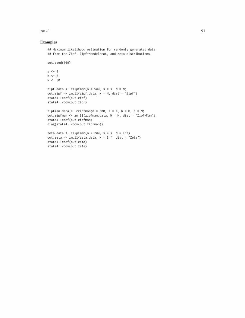
zm.ll 91

Examples

## Maximum likelihood estimation for randomly generated data## from the Zipf, Zipf-Mandelbrot, and zeta distributions.

set.seed(100)

s <- 2b <- 5N <- 50

zipf.data <- rzipfman(n = 500, s = s, N = N)out.zipf <- zm.ll(zipf.data, N = N, dist = "Zipf")stats4::coef(out.zipf)stats4::vcov(out.zipf)

zipfman.data <- rzipfman(n = 500, s = s, b = b, N = N)out.zipfman <- zm.ll(zipfman.data, N = N, dist = "Zipf-Man")stats4::coef(out.zipfman)diag(stats4::vcov(out.zipfman))

zeta.data <- rzipfman(n = 200, s = s, N = Inf)out.zeta <- zm.ll(zeta.data, N = Inf, dist = "Zeta")stats4::coef(out.zeta)stats4::vcov(out.zeta)

Index

∗Topic fileacc.samp, 4anovatol.int, 5bayesnormtol.int, 7bintol.int, 9bonftol.int, 12cautol.int, 13diffnormtol.int, 14DiffProp, 16DiscretePareto, 18distfree.est, 19dpareto.ll, 20dparetotol.int, 21exp2tol.int, 23exptol.int, 25exttol.int, 26F1, 28fidbintol.int, 29fidnegbintol.int, 31fidpoistol.int, 33gamtol.int, 35hypertol.int, 37K.factor, 38K.factor.sim, 40K.table, 42laptol.int, 44logistol.int, 45mvregtol.region, 47mvtol.region, 48negbintol.int, 50NegHypergeometric, 52neghypertol.int, 54nlregtol.int, 55norm.OC, 57norm.ss, 59normtol.int, 61np.order, 63npregtol.int, 64nptol.int, 66

paretotol.int, 68plottol, 69poislind.ll, 71poislindtol.int, 72PoissonLindley, 74poistol.int, 75regtol.int, 77simnormtol.int, 79TwoParExponential, 81umatol.int, 82uniftol.int, 83ZipfMandelbrot, 85zipftol.int, 87zm.ll, 89

.Random.seed, 17, 19, 53, 75, 81, 86

acc.samp, 4, 38, 55anova, 7anovatol.int, 5

bayesnormtol.int, 7, 60Binomial, 11, 83bintol.int, 9bonftol.int, 12

Cauchy, 14cautol.int, 13confint, 4

d2exp (TwoParExponential), 81ddiffprop (DiffProp), 16ddpareto (DiscretePareto), 18diffnormtol.int, 14DiffProp, 16, 28DiscretePareto, 18, 21, 22distfree.est, 19, 67dnhyper (NegHypergeometric), 52dpareto.ll, 20, 22dparetotol.int, 21dpoislind (PoissonLindley), 74

92

INDEX 93

dzipfman (ZipfMandelbrot), 85

exp2tol.int, 23, 69Exponential, 25exptol.int, 25exttol.int, 26

F1, 28fidbintol.int, 29, 32, 34fidnegbintol.int, 30, 31, 34fidpoistol.int, 30, 32, 33

GammaDist, 36gamtol.int, 35

Hypergeometric, 5, 38hypertol.int, 37

integrate, 28, 40, 41

K.factor, 7, 9, 15, 36, 38, 41, 43, 58, 62K.factor.sim, 40, 80K.table, 40, 42

laptol.int, 44lm, 7, 78loess, 65Logistic, 46logistol.int, 45

mle, 21, 72, 90mvregtol.region, 47mvtol.region, 48

NegBinomial, 52, 83negbintol.int, 50NegHypergeometric, 52, 55neghypertol.int, 54nlregtol.int, 55nls, 56norm.OC, 57norm.ss, 59Normal, 9, 15, 60, 62, 80normtol.int, 7–9, 15, 40, 58, 60, 61np.order, 63npregtol.int, 64, 67nptol.int, 20, 64, 65, 66

p2exp (TwoParExponential), 81paretotol.int, 68

pdiffprop (DiffProp), 16pdpareto (DiscretePareto), 18plottol, 69pnhyper (NegHypergeometric), 52poislind.ll, 71, 73poislindtol.int, 72Poisson, 77, 83PoissonLindley, 72, 73, 74poistol.int, 75ppoislind (PoissonLindley), 74pzipfman (ZipfMandelbrot), 85

q2exp (TwoParExponential), 81qdiffprop (DiffProp), 16qdpareto (DiscretePareto), 18qnhyper (NegHypergeometric), 52qpoislind (PoissonLindley), 74qzipfman (ZipfMandelbrot), 85

r2exp (TwoParExponential), 81rdiffprop (DiffProp), 16rdpareto (DiscretePareto), 18regtol.int, 77rnhyper (NegHypergeometric), 52rpoislind (PoissonLindley), 74runif, 17, 19, 53, 75, 81, 86rzipfman (ZipfMandelbrot), 85

simnormtol.int, 79spline, 65

TDist, 39–41tolerance (tolerance-package), 3tolerance-package, 3TwoParExponential, 24, 69, 81

umatol.int, 11, 52, 77, 82uniftol.int, 83

Weibull, 27

ZipfMandelbrot, 85, 89, 90zipftol.int, 87zm.ll, 89, 89

package ‘tolerance’ · tolerance-package 3 tolerance-package statistical tolerance intervals...

Documents