paciﬁc ocean: supplementary materials - caspo | scripps …ltalley/dpo/supplementary/ch_s1… ·...

C H A P T E R

S10

Pacific Ocean: Supplementary Materials

FIGURE S10.1 Pacific Ocean: mean surface geostrophic circulation with the current systems described in this text. Meansurface height (cm) relative to a zero global mean height, based on surface drifters, satellite altimetry, and hydrographicdata. (NGCUC ¼ New Guinea Coastal Undercurrent and SECC ¼ South Equatorial Countercurrent). Data from Niiler,

Maximenko, and McWilliams (2003).

1

FIGURE S10.2 Annual mean winds. (a) Wind stress (N/m2) (vectors) and wind-stress curl (�10�7 N/m3) (color),multiplied by �1 in the Southern Hemisphere. (b) Sverdrup transport (Sv), where blue is clockwise and yellow-red iscounterclockwise circulation. Data from NCEP reanalysis (Kalnay et al.,1996).

S10. PACIFIC OCEAN: SUPPLEMENTARY MATERIALS2

24.0

24.5

25.0

25.5

26.0

26.5

27.0

1

1

2

2

4810

12

121416

162025

3035 40

10

0

100

200

300

400

500

30°N 40°N 50°N

1 24

68

10 12

12

14

14

16

16

20

20

25

3035

40

4444

Dep

th (

m)

Latitude

Sea surface density

Pot

entia

l den

sity

σθ

Nitrate (μmol/kg)

Nitrate (μmol/kg)

(a)

(b)

(c)

(d)

0

100

200

300

400

500

44.5

5

5.5

6

6.5

78

8

9

1011

1213

1415

161718

9

3.5

0

100

200

300

400

500

33.8

33.9

34

34.134.2

34.5

34.1

34.3

32.733

33.7

32.8

34

3435.2 34.6

SAFZSTFZSubarctic DomainSubtropical Domain Transition Zone

30°N 40°N 50°N

Dep

th (

m)

Dep

th (

m)

SAFZSTFZ

Potential temperature

(°C)

Salinity

30°N 40°N 50°N

AlaskanStream

PF

FIGURE S10.3 The subtropical-subarctic transition along 150�W in the central North Pacific (MayeJune, 1984). SAFZand STFZ: subarctic and subtropical frontal zones. (a) Potential temperature (�C), (b) salinity, (c) nitrate (mmol/kg), and(d) nitrate versus potential density. After Roden (1991). Data from WOCE Pacific Ocean Atlas; Talley (2007).

S10. PACIFIC OCEAN: SUPPLEMENTARY MATERIALS 3

FIGURE S10.4 Subpolar gyre regimes. Only the major features are described in the text. Source: From Favorite, Dodimead,

and Nasu (1976).

FIGURE S10.5 Oyashio. Acceleration potential anomaly (similar to geopotential anomaly) on the isopycnal sq ¼ 26.52kg/m3 (150 cl/ton) referenced to 1500 dbar in September 1990. Source: From Kono and Kawasaki (1997).


FIGURE S10.6 (a) The Oyashio, Kuroshio, and Mixed Water Region east of Japan. (b) The southernmost latitude of thefirst Oyashio intrusion east of Honshu. Source: From Sekine (1999).


FIGURE S10.7 (a) Ocean color from the SeaWIFS satellite, showing an anticyclonic Haida Eddy in the Alaska Current onJune 13, 2002. Source: From NASAVisible Earth (2008). (b) Tracks of Sitka and Haida Eddies in 1995 and 1998 (top right) and inremaining years between 1993 and 2001 (bottom right). Source: From Crawford (2002).


FIGURE S10.8 Mean steric height at (a) 150 m and (b) 500 m relative to 2000 m; contour intervals are 0.04 and 0.02 m,respectively. Source: From Ridgway and Dunn (2003).


FIGURE S10.9 Sea level (m). (a) Total sea level, and(b) RMS sea level anomalies, from satellite altimetry. The3000 m isobath is shown (purple). Source: From Mata,

Wijffels, Church, and Tomczak (2006).

FIGURE S10.10 Surface chlorophyll concentration inaustral winter (June, July, August) and summer (December,January, February), derived from SeaWiFS satellite obser-vations. Source: From Mackas, Strub, Thomas, and Montecino

(2006).


FIGURE S10.11 Eastern South Pacific zonal vertical sections at 33�S: (a) temperature with meridional current directions,(b) salinity, (c) dissolved oxygen, and (d) phosphate.


FIGURE S10.12 RMS variability in surface height (cm) from satellite altimetry, high-passed with half power at 180 daysto depict the mesoscale eddy energy. �American Meteorological Society. Reprinted with permission. Source: From Qiu, Scott,

and Chen (2008).


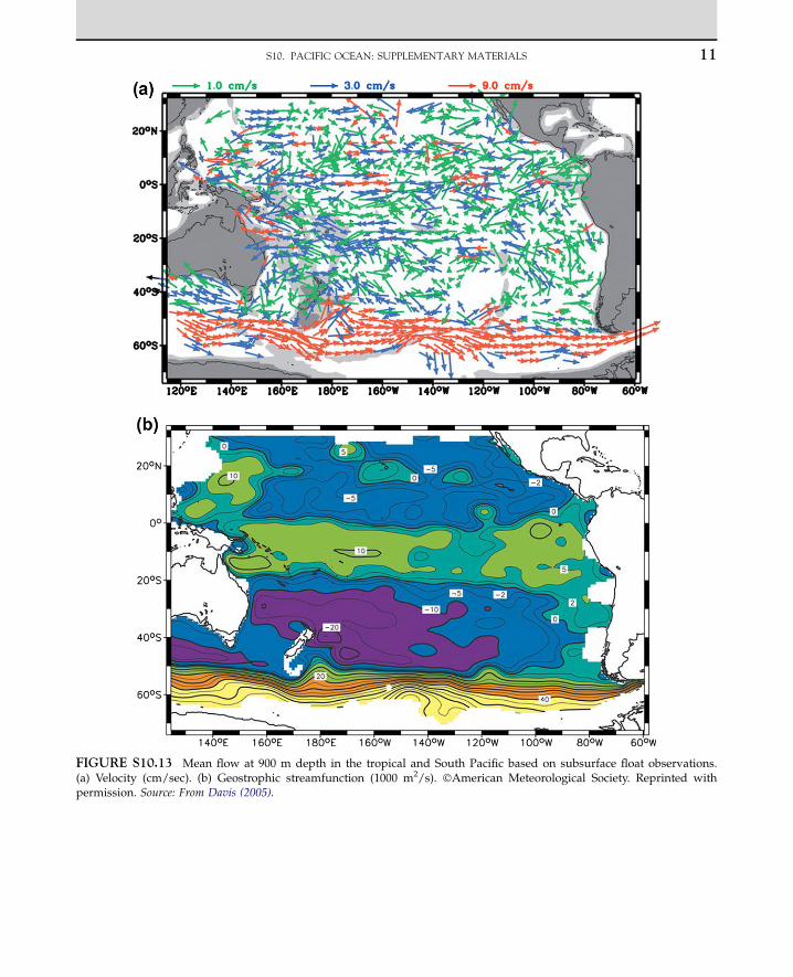
FIGURE S10.13 Mean flow at 900 m depth in the tropical and South Pacific based on subsurface float observations.(a) Velocity (cm/sec). (b) Geostrophic streamfunction (1000 m2/s). �American Meteorological Society. Reprinted withpermission. Source: From Davis (2005).


FIGURE S10.14 Pacific abyssal circulation schematics. Low latitude North Pacific. Source: From Kawabe, Yanagimoto, and

Kitagawa (2006).


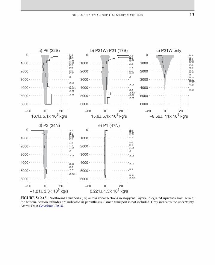
FIGURE S10.15 Northward transports (Sv) across zonal sections in isopycnal layers, integrated upwards from zero atthe bottom. Section latitudes are indicated in parentheses. Ekman transport is not included. Gray indicates the uncertainty.Source: From Ganachaud (2003).


100˚

100˚

120˚

120˚

140˚

140˚

160˚

160˚

180˚

180˚

200˚

200˚

220˚

220˚

240˚

240˚

260˚

260˚

280˚

280˚

300˚

300˚

-20˚ -20˚

0˚ 0˚

20˚ 20˚

00

0

0

0

0

100˚ 120˚ 140˚ 160˚ 180˚ 200˚ 220˚ 240˚ 260˚ 280˚ 300˚

-20˚ -20˚

0˚ 0˚

20˚ 20˚

0

0

0

00

0

00

0 0

August

0.1 N/m2

(a)

(b)

February

0-0.20 -0.10 0.10 0.20

Wind stress curl (N/m3)(x 1) (NH) or (x -1) (SH)

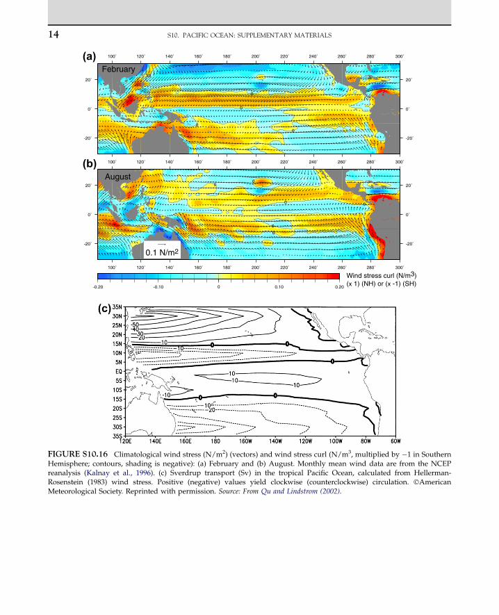
FIGURE S10.16 Climatological wind stress (N/m2) (vectors) and wind stress curl (N/m3, multiplied by �1 in SouthernHemisphere; contours, shading is negative): (a) February and (b) August. Monthly mean wind data are from the NCEPreanalysis (Kalnay et al., 1996). (c) Sverdrup transport (Sv) in the tropical Pacific Ocean, calculated from Hellerman-Rosenstein (1983) wind stress. Positive (negative) values yield clockwise (counterclockwise) circulation. �AmericanMeteorological Society. Reprinted with permission. Source: From Qu and Lindstrom (2002).


FIGURE S10.18 Chlorophyll composite images from SeaWiFS (January 1998 during El Nino and July 1998 duringtransition to La Nina). Red ¼ highest chlorophyll contents, dark purple ¼ lowest chlorophyll. Source: From SeaWiFS Project(2009).

FIGURE S10.17 Dynamic height (dyn cm) along the equator; transport (Sv) of the Equatorial Undercurrent is shown inthe inset. �American Meteorological Society. Reprinted with permission. Source: From Leetmaa and Spain (1981).


FIGURE S10.19 Currents in the western tropical Pacific. NEC ¼ North Equatorial Current; NECC ¼ North EquatorialCountercurrent; SEC ¼ South Equatorial Current; EUC ¼ Equatorial Undercurrent; NSCC and SSCC ¼ North and SouthSubsurface Countercurrent; MC ¼ Mindanao Current; MUC ¼ Mindanao Undercurrent; ME ¼ Mindanao Eddy; HE ¼Halmahera Eddy; NGCC ¼ New Guinea Coastal Current; NGCUC ¼ New Guinea Coastal Undercurrent; GBRUC ¼ GreatBarrier Reef Undercurrent; EAC ¼ East Australian Current; LC ¼ Leeuwin Current; AAIW ¼Antarctic Intermediate Water.Source: From Lukas, Yamagata, and McCreary (1996); after Fine et al. (1994).


FIGURE S10.20 Tropical sea surface temperature from the Tropical Rainfall Mapping Mission (TRMM) MicrowaveImager (TMI) for ten-day intervals from June 1 to August 30, 1998. Source: From Remote Sensing Systems (2004).


FIGURE S10.21 Winds and SST along the equator in the Pacific. Climatological zonal wind speed in (a) February and(b) August. Source: From TAO Project Office (2009b). (c) Monthly zonal wind speed (m/s) and SST (�C). Positive wind istowards the east. Source: From TAO Project Office (2009a).


(a)

FIGURE S10.22 (a) February mean winds (vectors) from COADS and February mean SST. The large arrows emphasizethe gaps through the American cordillera. From north to south: Tehuantepec, Papagayo, and Panama. Source: From Kessler

(2009). (b) SST in the Gulf of Tehuantepec, January 22, 1996. Source: From Zamudio et al. (2006).


-25-20-15-10

-505

10152025

SO

I (A

ustr

alia

BO

M)

1880 1890 1900 1910 1920 1930 1940 1950 1960 1970 1980 1990 2000

-15

Southern Oscillation Index (Australia BOM)

El Nino

La Nina

(a)

(b)

-2

0

2

Oceanic Nino Index (NOAA CPC)

1950 1955 1960 1965 1970 1975 1980 1985 1990 1995 2000 2005

Inde

x

El Nino

La Nina

FIGURE S10.23 (a) Southern Oscillation Index (SOI) time series from 1876 to 2008 (annual average). Data fromAustralian Government Bureau of Meteorology (2009). (b) “Oceanic Nino Index” based on SST in the region 5�Ne5�S,170�We120�W, as in Figure 10.28b. Red and blue in both panels correspond to El Nino and La Nina, respectively. (c) SSTreconstructions from the region 5�Ne5�S, 150�We 90�W. Source: From IPCC (2001). (d) Correlation of monthly sea levelpressure anomalies with the ENSO Nino3.4 index, averaged from 1948 to 2007. The Nino3.4 index is positive during theEl Nino phase, so the signs shown are representative of this phase. Data and graphical interface from NOAA ESRL (2009b).


FIGURE S10.23 (Continued).

FIGURE S10.24 Global precipitation anomalies for Northern Hemisphere summer (left) and winter (right) duringEl Nino. Source: From NOAA PMEL (2009d).


FIGURE S10.26 Subtropical Mode Water. (a) Vertical profile through North Pacific Subtropical Mode Water, at 29� 5’N,158� 33’E. Source: From Hanawa and Talley (2001). (b) North Pacific: thickness of the 17e18 �C layer. Source: From Masuzawa

(1969). (c) South Pacific: thickness of the 15e17 �C layer. �American Meteorological Society. Reprinted with permission.Source: From Roemmich and Cornuelle (1992).

FIGURE S10.25 Anomalies of United States winter (JFM) (a) temperature (�C) and (b) precipitation (mm) duringcomposite El Nino events from 1950 to 2008. Source: From NWS Internet Services Team (2008).


FIGURE S10.26 (Continued).

FIGURE S10.27 Salinity at the NPIW salinity minimum. Outer dark contour is the edge of the salinity minimum.�American Meteorological Society. Reprinted with permission. Source: From Talley (1993).


FIGURE S10.28 (a) Salinity, (b) oxygen (mmol/kg), and (c) silicate (mmol/kg) along 165�W. Neutral densities 28.00 and28.10 kg/m3 are superimposed. Station locations are shown in inset in (c). Source: From WOCE Pacific Ocean Atlas, Talley

(2007).


FIGURE S10.29 (a) Salinity, (b) silicate (mmol/kg), (c) D14C (/mille), and (d) d3He (%) at neutral density 28.01 kg/m3

(s2 ~ 36.96 kg/m3), characterizing PDW/UCDW at mid-depth. The depth of the surface is approximately 2600e2800 mnorth of the Antarctic Circumpolar Current. Source: From WOCE Pacific Ocean Atlas, Talley (2007).

FIGURE S10.30 (a) Salinity, (b) silicate (mmol/kg), and (c) depth (m) at neutral density 28.10 kg/m3 (s4 ~ 45.88 kg/m3),characteristic of LCDW. (d) Potential temperature at 4000 m. Source: From WOCE Pacific Ocean Atlas, Talley (2007).


TABLE S10.1 Major Upper Ocean Circulation Systems, Currents and Fronts of the Mid and High Latitude NorthPacific (Figure S10.1)*

Name Description Approximate Location

Subtropical gyre Anticyclonic gyre at mid-latitudes 10e40�N

Subpolar gyre Cyclonic gyre at mid to high latitudes 40e65�N

Western Subarctic Gyre Intense cyclonic sub-gyre in the western subpolar gyre 40e55�N, Kuril Islands to180�

Alaska Gyre Intense cyclonic sub-gyre in the eastern subpolar gyre 40�N to Alaskan coast, 180�

to eastern boundary

Bering Sea gyre Cyclonic circulation in the Bering Sea Bering Sea

Okhotsk Sea gyre Cyclonic circulation in the Okhotsk Sea Okhotsk Sea

Kuroshio Subtropical western boundary current 12e35�N

Kuroshio Extension Subtropical western boundary current extension 35�N

Kuroshio recirculation orKuroshio Countercurrent

Westward flow just south of the Kuroshio Extension 30�N

Subtropical Countercurrent Eastward flow of the western subtropical gyre, south ofthe recirculation; continues into the Subtropical Front

25�N

California Current System Subtropical eastern boundary current system 23e52�N

Oyashio Subpolar western boundary current south of centralKuril Islands

40eN

East Kamchatka Current Subpolar western boundary current north of centralKuril Islands

45e65�N

Alaska Current Subpolar eastern boundary current North of 52�N

Alaskan Stream Southwestward flow of the subpolar gyre along thenorthern boundary

180e145�W

North Equatorial Current Westward flow of the subtropical gyre and northerntropical gyre

10e20�N

North Pacific Current Eastward flow of the subtropical and subpolar gyres 20e50�N

Subtropical Frontal Zone Zonal frontal band in the subtropical gyre; close to themaximum Ekman transport convergence

30e35�N

Subarctic Frontal Zone Zonal frontal band separating the subpolar and subtropicalgyre regimes; close to maximum westerly wind stress

40e�N

* Shading indicates the basic set.


TABLE S10.2 South Pacific Circulation Systems and Currents*

Name Description

Subtropical gyre Anticyclonic gyre at mid-latitudes

East Australian Current (EAC) Western boundary current of the subtropical gyre along the coastof Australia

Tasman Front Eastward current connecting the East Australian Current and theEast Auckland Current

East Auckland Current Western boundary current of the subtropical gyre along the coast ofNew Zealand

South Pacific Current (or Westwind Drift) Eastward flow of the subtropical gyre

Subantarctic Front (SAF) Eastward flow in the northernmost front of the AntarcticCircumpolar Current

Peru-Chile Current System (PCCS) Eastern boundary current system for the subtropical gyre

Peru-Chile Current (PCC) Northward flow in the PCCS

Poleward Undercurrent (PUC) Southward undercurrent in the PCCS

Peru-Chile Countercurrent (PCCC) Southward surface flow within the PCCS

Cape Horn Current Southward eastern boundary current

South Equatorial Current Westward flow of the subtropical gyre



TABLE S10.3 Tropical Pacific Currents*

Name Description

Location Upper Ocean

Unless Otherwise Noted

North Equatorial Current (NEC) Westward flow of the North Pacificsubtropical gyre

8e30�N

South Equatorial Current (SEC) Westward flow of the South Pacificsubtropical gyre and westward flow in theequatorial region

30�S to 3�N

North Equatorial Countercurrent (NECC) Eastward flow between the NEC and SEC 3e8�N

South Equatorial Countercurrent (SECC) Eastward flow embedded in the SEC 8e11�S, western andcentral Pacific only

Equatorial Undercurrent (EUC) Eastward subsurface flow, just below thesurface layer

1�S to 1�N50e250 m

Equatorial Intermediate Current (EIC) Westward subsurface flow, below the EUC 1�S to 1�N250e1000 m

Equatorial stacked jets Reversing subsurface eastward-westwardjets, beneath the EIC

1�S to 1�N1000 m to bottom

North and South Subsurface Countercurrents(NSCC, SSCC; “Tsuchiya jets”)

Eastward subsurface flows, off the equator 6e2�S; 2e6�N150e500 m

Mindanao Current Southward western boundary currentconnecting the NEC and NECC

6e14�N

New Guinea Coastal Undercurrent (NGCUC) Northward tropical western boundarycurrent connecting the SEC and NQC tothe EUC, NSCC and SSCC

12�S to 6�N

North Queensland Current (NQC) and GreatBarrier Reef Undercurrent (GBRUC)

Northward western boundary current forthe SEC

15e12�S (NQC)23e15�S (GBRUC)



TABLE S10.4 Principal Pacific Ocean Water Masses*

Water Mass Characteristic in the Vertical Layer Process

North Pacific Central Water(NPCW)

Subtropical thermocline waters Upper0e1000 m

Subduction

South Pacific Central Water(SPCW)

Subtropical thermocline waters Upper0e1000 m

Subduction

North Pacific SubtropicalUnderwater (NPSTUW)

Subtropical/tropical salinitymaximum

Upper100e200 m

Subduction of high salinitysubtropical surface waters

South Pacific SubtropicalUnderwater (SPSTUW)

Subtropical/tropical salinitymaximum

Upper100e200 m

Subduction of high salinitysubtropical surface waters

North Pacific SubtropicalMode Water (NPSTMW)

Subtropical stability (potentialvorticity) minimum

Upper0e400 m

Subduction of thick winter mixedlayer

South Pacific SubtropicalMode Water (SPSTMW)

Subtropical stability (potentialvorticity) minimum

Upper0e300 m

Subduction of thick winter mixedlayer

Subantarctic Mode Water(SAMW)

Southern subtropical stability(potential vorticity) minimum

Upper0e600 m

Subduction of thick winter mixedlayer from Subantarctic Front

Dichothermal Water (DtW) North Pacific subpolartemperature minimum

Upper0e150 m

Advection of cold subpolar surfacewaters

Mesothermal Water (MtW) North Pacific subpolartemperature maximum

Upper200e500 m

Advection of warmer near-surfacesubpolar waters

North Pacific IntermediateWater (NPIW)

Salinity minimum in subtropicalNorth Pacific

Intermediate200e800 m

Advection of fresh subpolar surfacewater

Antarctic Intermediate Water(AAIW)

Salinity minimum in subtropicalNorth Pacific and tropical Pacific

Intermediate500e1200 m

Advection of fresh subantarcticsurface water

Pacific Deep Water (PDW) Oxygen minimum, nutrientmaximum

Deep1000e4000 m

Mixing and aging of deep waters

Upper Circumpolar DeepWater (UCDW)

High oxygen, low nutrients, highsalinity on isopycnal surfaces

Deep~ 1000e3000 m

Mixture of deep waters in theSouthern Ocean

Lower Circumpolar DeepWater (LCDW)

Deep salinity and oxygenmaxima, nutrient minima

Bottom3000m to bottom

Brine rejection in the Southern Oceanmixed with NADW, PDW, and IDW




References

Australian Government Bureau of Meteorology, 2009. S.O.I(Southern Oscillation Index) Archivesd 1876 to present.http://reg.bom.gov.au/climate/current/soihtm1.shtml(accessed 03.27.09).

Crawford, W., 2002. Physical characteristics of HaidaEddies. J. Oceanogr 58, 703e713.

Davis, R.E., 2005. Intermediate-depth circulation of theIndian and South Pacific Oceans measured by autono-mous floats. J. Phys. Oceanogr 35, 683e707.

Favorite, F., Dodimead, A.J., Nasu, K., 1976. Oceanog-raphy of the subarctic Pacific region, 1960e71. Inter-national North Pacific Fisheries Commission, ew, 33,187 pp.

Fine, R.A., Lukas, R., Bingham, F.M., Warner, M.J.,Gammon, R.H., 1994. The western equatorial Pacific:A water mass crossroads. J. Geophys. Res. 99,25063e25080.

Ganachaud, A., 2003. Large-scale mass transports, watermass formation, and diffusivities estimated from WorldOcean Circulation Experiment (WOCE) hydrographicdata. J. Geophys. Res. 108 (C7), 3213. doi: 10.1029/2002JC002565.

Hanawa, K., Talley, L.D., 2001. Mode Waters. In: Siedler, G.,Church, J. (Eds.), Ocean Circulation and Climate. Inter-national Geophysics Series. Academic Press,pp. 373e386.

IPCC, 2001. Climate Change 2001: The Scientific Basis. In:Houghton, J.T., Ding, Y., Griggs, D.J., Noguer, M., vander Linden, P.J., Dai, X., Maskell, K., Johnson, C.A.(Eds.), Contribution of Working Group I to the ThirdAssessment Report of the Intergovernmental Panel onClimate change. Cambridge University Press, Cam-bridge, UK and New York, 881 pp.

Kalnay, E., Kanamitsu, M., Kistler, R., Collins, W.,Deaven, D., Gandin, L., 1996. The NCEP-NCAR 40-yearreanalysis project. B. Am. Meteorol. Soc. 77, 437e471.

Kawabe, M., Yanagimoto, D., Kitagawa, S., 2006. Variations ofdeep western boundary currents in the Melanesian Basinin the western North Pacific. Deep-Sea Res. I 53, 942e959.

Kessler, W.S., 2009. The Central American mountain-gap winds and their effects on the ocean. http://faculty.washington.edu/kessler/t-peckers/t-peckers.html(accessed 3.27.09).

Kono, T., Kawasaki, Y., 1997. Modification of the westernsubarctic water by exchange with the Okhotsk Sea.Deep-Sea Res. I 44, 689e711.

Leetmaa, A., Spain, P.F., 1981. Results from a velocitytransect along the equator from 125 to 159�W. J. Phys.Oceanogr. 11, 1030e1033.

Lukas, R., Yamagata, T., McCreary, J.P., 1996. Pacific low-latitude western boundary currents and the Indonesianthroughflow. J. Geophys. Res. 101, 12209e12216.

Mackas, D.L., Strub, P.T., Thomas, A., Montecino, V., 2006.Eastern ocean boundaries pan-regional overview. In:Robinson, A.R., Brink, K.H. (Eds.), The Sea, Vol. 14A:The Global Coastal Ocean: Interdisciplinary RegionalStudies and Syntheses. Harvard University Press,pp. 21e60.

Masuzawa, J., 1969. Subtropical Mode Water. Deep-Sea Res.16, 453e472.

Mata, M.M., Wijffels, S.E., Church, J.A., Tomczak, M., 2006.Eddy shedding and energy conversions in the EastAustralian Current. J. Geophys. Res. 111, C09034.doi:10.1029/2006JC003592.

McClain, C., Christian, J.R., Signorini, S.R., Lewis, M.R.,Asanuma, I., Turk, D., Dupouy-Douchement, C., 2002.Satellite ocean-color observations of the tropical PacificOcean. Deep-Sea Res. II 49, 2533e2560.

NASA Visible Earth, 2008. Eddies off the Queen CharlotteIslands. NASA Goddard Space Flight Center. http://visibleearth.nasa.gov/view_rec.php?id=2886 (accessed3.26.09).

Niiler, P.P., Maximenko, N.A., McWilliams, J.C., 2003.Dynamically balanced absolute sea level of the globalocean derived from near-surface velocity observations.Geophys. Res. Lett. 30, 22. doi:10.1029/2003GL018628.

NOAA ESRL, 2009b. Linear correlations in atmosphericseasonal/monthly averages. NOAA Earth SystemResearch Laboratory Physical Sciences Division. http://www.cdc.noaa.gov/data/correlation/ (accessed 10.30.09).

NOAA PMEL, 2009d. Impacts of El Nino and benefits ofEl Nino prediction. NOAA Pacific Marine Environ-mental Laboratory. http://www.pmel.noaa.gov/tao/elnino/impacts.html (accessed 3.26.09).

NWS Internet Services Team, 2008. ENSO temperature andprecipitation composites. http://www.cpc.noaa.gov/products/precip/CWlink/ENSO/composites/EC_LNP_index.shtml (accessed 3.27.09).

Qiu, B., Scott, R.B., Chen, S., 2008. Length scales of eddygeneration and nonlinear evolution of the seasonallymodulated South Pacific Subtropical Countercurrent.J. Phys. Oceanogr. 38, 1515e1528.

Qu, T., Lindstrom, E., 2002. A climatological interpretationof the circulation in the western South Pacific. J. Phys.Oceanogr. 32, 2492e2508.

Remote Sensing Systems, 2004. TMI sea surface tempera-tures (SST). http://www.ssmi.com/rss_research/tmi_sst_pacific_equatorial_current.html (accessed 3.27.09).

Ridgway, K.R., Dunn, J.R., 2003. Mesoscale structure of themean East Australian Current System and its relation-ship with topography. Progr. Oceanogr. 56, 189e222.

Roden, G.I., 1991. Subarctic-subtropical transition zone ofthe North Pacific: Large-scale aspects and mesoscalestructure. In: Wetherall, J.A. (Ed.), Biology, Oceanog-raphy and Fisheries of the North Pacific Transition Zone


and the Subarctic Frontal Zone. NOAATechnical Report105, 1e38.

Roemmich, D., Cornuelle, B., 1992. The Subtropical ModeWaters of the South Pacific Ocean. J. Phys. Oceanogr. 22,1178e1187.

SeaWiFS Project, 2009. SeaWiFS captures El Nino-La Ninatransitions in the equatorial Pacific. NASA GoddardSpace Flight Center. http://oceancolor.gsfc.nasa.gov/SeaWiFS/BACKGROUND/Gallery/pac_elnino.jpg(accessed 3.26.09).

Sekine, Y., 1999. Anomalous southward intrusions of theOyashio east of Japan 2. Two-layer numerical model.J. Geophys. Res. 104, 3049e3058.

Talley, L.D., 1993. Distribution and formation of NorthPacific Intermediate Water. J. Phys. Oceanogr 23,517e537.

Talley, L.D., 2007. Hydrographic Atlas of the World OceanCirculation Experiment (WOCE). In: Sparrow, M.,Chapman, P., Gould, J. (Eds.), Pacific Ocean, Volume 2.International WOCE Project Office, Southampton, U.K.ISBN 0-904175-54-5.

TAO Project Office, 2009a. TAO/TRITON data display anddelivery. NOAA Pacific Marine Environmental Labora-tory. http://www.pmel.noaa.gov/tao/disdel/disdel.html (accessed 3.27.09).

TAO Project Office, 2009b. TAO Climatologies. NOAAPacific Marine Environmental Laboratory. http://www.pmel.noaa.gov/tao/clim/clim.html (accessed 7.5.09).

Zamudio, L., Hurlburt, H.E., Metzger, E.J., Morey, S.L.,O’Brien, J.J., Tilburg, C.E., Zavala-Hidalgo, J., 2006.Interannual variability of Tehuantepec eddies. J. Geo-phys. Res. 111, C05001. doi:10.1029/2005JC003182.

paciﬁc ocean: supplementary materials - caspo | scripps …ltalley/dpo/supplementary/ch_s1… ·...

Documents