opto-acoustic slopping prediction system in basic oxygen

IN DEGREE PROJECT INFORMATION AND COMMUNICATION TECHNOLOGY,SECOND CYCLE, 30 CREDITS

, STOCKHOLM SWEDEN 2017

Opto-Acoustic Slopping Prediction System in Basic Oxygen Furnace Converters

BINAYAK GHOSH

KTH ROYAL INSTITUTE OF TECHNOLOGYSCHOOL OF INFORMATION AND COMMUNICATION TECHNOLOGY

Acknowledgement

I would first like to thank my thesis advisors Norbert Uebber and Dr. Hans-JürgenOdenthal at SMS group GmbH for giving me this opportunity, facilities and supportneeded to complete this thesis. I wish to express my sincere gratitude to DimitriosStathis and Syed Asad Jafri at KTH Royal Institute of Technology for being mysupervisors and providing necessary guidance throughout the project. I am alwaysthankful to them for giving me the intellectual freedom, supporting my ideas anddemanding a high quality work in all my endeavors.

With deep sense of gratitude I thank Professor Ahmed Hemani at KTH RoyalInstitute of Technology for offering me the support and keeping the door open when-ever I had question regarding my research. I am gratefully indebted to him for thevery valuable comments on this thesis.

I am always thankful to my Grandmother, Mother and Father for the everlastinglove and support, without whom I would not be able to be in this position in thefirst place. This accomplishment would not have been possible without my friends,who have always motivated me and helped me whenever I needed them and I amforever indebted to them.

Opto-Acoustic Slopping Prediction System in BasicOxygen Furnace Converters

Binayak Ghosh

October 25, 2017

Abstract

Today, everyday objects are becoming more and more intelligent andsome-times even have self-learning capabilities. These self-learning capacitiesin particular also act as catalysts for new developments in the steel indus-try.Technical developments that enhance the sustainability and productivityof steel production are very much in demand in the long-term. The methodsof Industry 4.0 can support the steel production process in a way that enablessteel to be produced in a more cost-effective and environmentally friendlymanner.

This thesis describes the development of an opto-acoustic system for theearly detection of slag slopping in the BOF (Basic Oxygen Furnace) converterprocess. The prototype has been installed in Salzgitter Stahlwerks, a Germansteel plant for initial testing. It consists of an image monitoring camera at theconverter mouth, a sound measurement system and an oscillation measure-ment device installed at the blowing lance. The camera signals are processedby a special image processing software. These signals are used to rate theamount of spilled slag and for a better interpretation of both the sound dataand the oscillation data. A certain aspect of the opto-acoustic system for slop-ping detection is that all signals, i.e. optic, acoustic and vibratory, are affectedby process-related parameters which are not always relevant for the sloppingevent. These uncertainties affect the prediction of the slopping phenomenaand ultimately the reliability of the entire slopping system. Machine Learningalgorithms have been been applied to predict the Slopping phenomenon basedon the data from the sensors as well as the other process parameters.

Keywords - BOF, Slopping, Sensor fusion, Image Processing, MachineLearning, Data Analysis, Neural Networks, Deep Learning

i

Sammanfattning

Idag blir vardagliga föremål mer och mer intelligenta och ibland har de självlärandemöjligheter. Dessa självlärande förmågor fungerar också som katalysatorer förden nya utvecklingen inom stålindustrin. Teknisk utveckling som stärker håll-barheten och produktiviteten i stålproduktionen är mycket efterfrågad på lång sikt.Metoderna för Industry 4.0 kan stödja stålproduktionsprocessen på ett sätt som göratt stål kan produceras på ett mer kostnadseffektivt och miljövänligt sätt.

Denna avhandling beskriver utvecklingen av ett opto-akustiskt system för tidigdetektering av slaggsslipning i konverteringsprocessen BOF (Basic Oxygen Furnace).Prototypen har installerats i Salzgitter Stahlwerks, en tysk stålverk för första provn-ing. Den består av en bildövervakningskamera på omvandlarens mun, ett ljudmät-ningssystem och en oscillationsmätningsenhet som installeras vid blåsans. Kameranssignaler behandlas av en speciell bildbehandlingsprogram. Dessa signaler användsför att bestämma mängden spilld slagg och för bättre tolkning av både ljuddataoch oscillationsdata. En viss aspekt av det optoakustiska systemet för släcknings-detektering är att alla signaler, dvs optiska, akustiska och vibrerande, påverkas avprocessrelaterade parametrar som inte alltid är relevanta för slöjningsevenemanget.Dessa osäkerheter påverkar förutsägelsen av slopfenomenerna och i slutändan tillför-litligheten för hela slöjningssystemet. Maskininlärningsalgoritmer har tillämpats föratt förutsäga Slopping-fenomenet baserat på data från sensorerna liksom de andraprocessparametrarna.

Keywords - BOF, Slopping, Sensorfusion, Bildbehandling, Maskininlärning,Dataanalys, Neurala nätverk, Deep Learning

ii

ContentsAbstract i

Contents iv

List of figures vi

List of tables vii

1 Introduction 11.1 Background . . . . . . . . . . . . . . . . . . . . . . . . . . . . . . . . . 11.2 Motivation . . . . . . . . . . . . . . . . . . . . . . . . . . . . . . . . . 21.3 Purpose . . . . . . . . . . . . . . . . . . . . . . . . . . . . . . . . . . . 21.4 Scope of Thesis . . . . . . . . . . . . . . . . . . . . . . . . . . . . . . . 21.5 Thesis Outline . . . . . . . . . . . . . . . . . . . . . . . . . . . . . . . 3

2 Literature study 42.1 Industrial Internet of Things and Big Data Analytics . . . . . . . . . 42.2 Internet of Things in Steel Manufacturing . . . . . . . . . . . . . . . . 52.3 The BOF Converter Process . . . . . . . . . . . . . . . . . . . . . . . 52.4 Related works on Slopping Prevention Techniques . . . . . . . . . . . 8

3 Machine learning theory 103.1 Machine learning . . . . . . . . . . . . . . . . . . . . . . . . . . . . . . 103.2 Performance metrics for classification methods . . . . . . . . . . . . . 103.3 Decision Trees . . . . . . . . . . . . . . . . . . . . . . . . . . . . . . . 113.4 Random Forest . . . . . . . . . . . . . . . . . . . . . . . . . . . . . . . 123.5 Single Layer Neural Network . . . . . . . . . . . . . . . . . . . . . . . 12

3.5.1 Artificial Neurons . . . . . . . . . . . . . . . . . . . . . . . . . . 123.5.2 Single-Layer Feedforward Networks . . . . . . . . . . . . . . . . 13

3.6 The Perceptron . . . . . . . . . . . . . . . . . . . . . . . . . . . . . . . 143.7 Multilayer Neural networks . . . . . . . . . . . . . . . . . . . . . . . . 15

3.7.1 The Multilayer Perceptron . . . . . . . . . . . . . . . . . . . . . 153.8 Deep Learning . . . . . . . . . . . . . . . . . . . . . . . . . . . . . . . 16

3.8.1 Activation and Loss Functions . . . . . . . . . . . . . . . . . . . 163.8.2 Regularization . . . . . . . . . . . . . . . . . . . . . . . . . . . . 17

4 Implementation 184.1 Design of Optical Measuring System . . . . . . . . . . . . . . . . . . . 18

4.1.1 Experimental setup . . . . . . . . . . . . . . . . . . . . . . . . . 184.1.2 Video Processing Algorithm . . . . . . . . . . . . . . . . . . . . 20

4.2 Design of Acoustic Measuring System . . . . . . . . . . . . . . . . . . 23

iii

CONTENTS

4.3 Design of Vibration Measuring System . . . . . . . . . . . . . . . . . . 254.4 System Setup . . . . . . . . . . . . . . . . . . . . . . . . . . . . . . . . 28

4.4.1 Installation of microphones and camera . . . . . . . . . . . . . . 294.5 Data . . . . . . . . . . . . . . . . . . . . . . . . . . . . . . . . . . . . . 30

4.5.1 Static Data . . . . . . . . . . . . . . . . . . . . . . . . . . . . . . 314.5.2 Dynamic Data . . . . . . . . . . . . . . . . . . . . . . . . . . . . 314.5.3 Preparation of Data . . . . . . . . . . . . . . . . . . . . . . . . . 32

4.6 Modeling . . . . . . . . . . . . . . . . . . . . . . . . . . . . . . . . . . 344.6.1 Selection of features . . . . . . . . . . . . . . . . . . . . . . . . . 34

5 Results and Analysis 375.1 Decision Tree . . . . . . . . . . . . . . . . . . . . . . . . . . . . . . . . 375.2 Random Forest . . . . . . . . . . . . . . . . . . . . . . . . . . . . . . . 395.3 Deep Learning . . . . . . . . . . . . . . . . . . . . . . . . . . . . . . . 40

5.3.1 H2O . . . . . . . . . . . . . . . . . . . . . . . . . . . . . . . . . 405.3.2 Deep learning in H2O . . . . . . . . . . . . . . . . . . . . . . . . 40

5.4 Final Comparison of Models . . . . . . . . . . . . . . . . . . . . . . . . 455.5 Implementation of model in server for online testing . . . . . . . . . . 46

6 Conclusions and Discussion 49

iv

List of Figures2.1 Oxygen is blown through the lance of the converter vessel and an emul-

sion of gas, metal and slag is formed . . . . . . . . . . . . . . . . . . . 62.2 Phenomenon of slopping occurrence due to overflow of slag in the con-

verter . . . . . . . . . . . . . . . . . . . . . . . . . . . . . . . . . . . . 73.1 An example of a decision tree to predict slopping outcome from the

static parameter values . . . . . . . . . . . . . . . . . . . . . . . . . . 113.2 Nonlinear model of a neuron . . . . . . . . . . . . . . . . . . . . . . . 133.3 Single-Layer Feedforward Network . . . . . . . . . . . . . . . . . . . . 143.4 Figure a) showing separable patterns, where the two regions can be

separated by a linear function, while, in Figure b), such separation isnot possible . . . . . . . . . . . . . . . . . . . . . . . . . . . . . . . . . 14

3.5 Multilayer Feedforward Network . . . . . . . . . . . . . . . . . . . . . 154.1 Optical measuring system: network-capable camera for the digital de-

tection of slopping at the converter mouth. . . . . . . . . . . . . . . . 184.2 Experimental setup of camera system to detect slopping occurrence at

the BOF converter . . . . . . . . . . . . . . . . . . . . . . . . . . . . . 194.3 Images of slopping captured by the camera system . . . . . . . . . . . 204.4 Original image of the converter mouth with sparks and small, adhering

slag part at the right edge (right) and Result image with recognizedslag part at the converter (left) . . . . . . . . . . . . . . . . . . . . . . 20

4.5 Algorithm used for detecting the bright pixels in the captured images 214.6 Detection of incandescent material from the captured image by the

camera to detect illuminated slag particles . . . . . . . . . . . . . . . . 214.7 Figure on the right is generated by applying the thresholding mask on

the input image on the left on the as captured by the camera system . 224.8 The mask is then applied to ignore the zone with the contents of the

converter . . . . . . . . . . . . . . . . . . . . . . . . . . . . . . . . . . 224.9 This figure shows the trajectory of a the sound signal over the duration

of a heat, when the level of the sound signal crosses the threshold de-marcated by the red line, it indicates that there is a certain probabilityof occurrence of slopping . . . . . . . . . . . . . . . . . . . . . . . . . . 24

4.10Overview of the sound monitoring system which includes two micro-phones attached to the top (at 19m height) and base of the convertervessel . . . . . . . . . . . . . . . . . . . . . . . . . . . . . . . . . . . . 25

4.11 Schematic of the vibration measurement installation setup at the BOFconverter to detect slopping occurrence . . . . . . . . . . . . . . . . . . 26

v

LIST OF FIGURES

4.12Vibration pattern during a heat, corresponds to the patterns of theoxygen rate, lance height and the number of bright pixels; the areain the green zone shows an instance where a peak in the vibrationpattern is also reflected by a corresponding change in the patterns ofthe oxygen rate, lance height and the number of bright pixels . . . . . 27

4.13 Layout of the system at SZFG Salzgitter . . . . . . . . . . . . . . . . . 284.14Microphone attachment outside wall in the north east . . . . . . . . . 294.15 Installation of the camera System . . . . . . . . . . . . . . . . . . . . . 304.16 Sample dataset consisting of dynamic data of heat numbered 72638 as

measured on 16.01.2017 . . . . . . . . . . . . . . . . . . . . . . . . . . 314.17Acoustic plot depicting sound level variations in an average slopping

heat; the black line shows the heat with no slopping, the red line showsthe heat with liquid slopping and the blue line depicts the heat withsolid slopping . . . . . . . . . . . . . . . . . . . . . . . . . . . . . . . . 33

4.18 Plot of bright pixels against time in an average slopping heat; the blackline shows the heat with no slopping, the red line shows the heat withliquid slopping and the blue line depicts the heat with solid slopping . 33

4.19Chart of Importance Ratings of the Variables, as calculated using acombination of the ’Select K Best’, ’Randomized Lasso’, and ’BayesianRegression with ARD’, applied on all 2500 heats collected from Marchto June . . . . . . . . . . . . . . . . . . . . . . . . . . . . . . . . . . . 36

5.1 Confusion Matrix for implementation of decision tree algorithm to pre-dict slopping occurrence;the slopping categories [0], [1], [2], [3] and [4]are predicted, with [0] indicating no slopping, and [4] indicating max-imum slopping; the vertical rows depict the actual values while thehorizontal rows show the predicted values by the algorithm . . . . . . . 38

5.2 Confusion Matrix for Implementation of random forest algorithm topredict slopping occurrence;the slopping categories [0], [1], [2], [3] and[4] are predicted, with [0] indicating no slopping, and [4] indicatingmaximum slopping; the vertical rows depict the actual values whilethe horizontal rows show the predicted values by the algorithm . . . . 39

5.3 Table showing a plot of the variation of the mean squared error (MSE)for different number of hidden nodes, in the H2O deep learning model,calculated using the training dataset . . . . . . . . . . . . . . . . . . . 42

5.4 Comparison of variance of accuracy distribution of cross-validationmetrics of three models, decision trees, random forests and deep learn-ing . . . . . . . . . . . . . . . . . . . . . . . . . . . . . . . . . . . . . 46

5.5 Rapidminer Studio and Rapidminer Server Architecture . . . . . . . . 475.6 Graphical User Interface for online execution of Predictive Model for

Slopping Detection . . . . . . . . . . . . . . . . . . . . . . . . . . . . . 48

vi

List of Tables1 Activation functions for the deep learning methods [1] . . . . . . . . . 172 Loss functions for the deep learning methods [1] . . . . . . . . . . . . 173 Features of H2O cluster that was setup for building the predictive model 424 Results of application of deep learning model on test data, showing the

mean squared error (MSE), the root mean squared error (RMSE), thelogloss of the model and the mean error per class . . . . . . . . . . . . 43

5 Confusion matrix for implementation of deep learning algorithm topredict slopping occurrence;the slopping categories [0], [1], [2], [3] and[4] are predicted, with [0] indicating no slopping, and [4] indicatingmaximum slopping; the vertical rows depict the actual values whilethe horizontal rows show the predicted values by the algorithm . . . . 43

6 Table showing the full scoring history of the H2O deep learning algo-rithm on the test data which includes the duration per iteration, thetraining speed of the model, the number of predictions made and theclassification error . . . . . . . . . . . . . . . . . . . . . . . . . . . . . 44

7 Results of application of deep learning model using cross-validation,showing the mean squared error (MSE), the root mean squared error(RMSE), the logloss of the model and the mean error per class . . . . 44

8 Confusion matrix for implementation of deep learning algorithm, usingcross-validation, to predict slopping occurrence;the slopping categories[0], [1], [2], [3] and [4] are predicted, with [0] indicating no slopping,and [4] indicating maximum slopping; the vertical rows depict the ac-tual values while the horizontal rows show the predicted values by thealgorithm . . . . . . . . . . . . . . . . . . . . . . . . . . . . . . . . . . 45

9 Metrics Summary for the deep learning model after cross-validation . . 4510 Comparison of the developed system with the existing methods . . . . 51

vii

1 INTRODUCTION

1 | IntroductionThe Internet of Things (IoT) has transformed the physical world into a type of in-formation system — through sensors and actuators embedded in physical objectsand linked through wired and wireless networks via the Internet Protocol. In manu-facturing, the pertinence for cyber-physical systems to improve productivity in theproduction process and the supply chain is vast. ’Industrie 4.0’ is a German gov-ernment initiative that promotes automation of the manufacturing industry withthe goal of developing Smart Factories. McKinsey defines Industry 4.0 as "digiti-zation of the manufacturing sector, with embedded sensors in virtually all productcomponents and manufacturing equipment, ubiquitous cyberphysical systems, andanalysis of all relevant data" [2].

The direct fallout of the Internet of Things is Big Data Analytics or simply BigData. Advanced analytics refers to the use of statistical and mathematical toolsand formulae to data in order to obtain actionable insights which help to improveand optimize business operations. In the manufacturing sector, managers can useanalytics methods to delve into the historical process data and identify patterns, andrelationships among the process data and then, use it to optimize plant processes,to improve yield and productivity [2].

One of the prime examples in this regard is the Steel Industry. Steel is ubiquitous,everything is made from steel to some extent. It is an indispensable material formodern transportation infrastructure. A considerable number of people work insteel-intensive industries in Germany alone. And steel is a high-tech product thatgenerates huge masses of data in its processing — Big Steel Data [3].

1.1 BackgroundSteelmaking in the Basic Oxygen Furnace (BOF) [4] is a primary steelmaking processfor converting the molten pig iron into steel by blowing oxygen through a lance overthe molten pig iron inside the converter.

The formation of slag is a vital part of the BOF process. Slag, along with theother chemical compositions inside the converter, together, produce an emulsionwhich acts as the site for the essential metallurgical reactions. Proper slag foamingrequires a good conversion of materials. However, under some process conditions thefoamy slag volume becomes so large that it is thrown out of the converter. Sloppingprocesses must be avoided because they reduce yield and productivity, and mightdamage components.

As described in [5], Slopping is "the technical term used in steelmaking to describethe event when the slag foam cannot be contained within the process vessel, butis forced out through its opening. Slopping reduces process yields and may lead to

1

1 INTRODUCTION

discharge of pollutants to the surrounding environment."With increasing computing power, data storage capacity, advanced algorithms

and innovative sensor technologies it is today possible to apply machine learning anddata driven prediction models in the BOF process. These approaches process largeamounts of data to predict the BOF process conditions, one of the most essential ofwhich is slopping.

1.2 MotivationSlopping causes operational and environmental problems in basic oxygen steelmak-ing. The detection of the occurrence of slopping using a slop detection system is oneof the ways by which slopping can be prevented. Thus it is imperative to design asystem which will be able to detect and predict the slopping occurrences.

1.3 PurposeThe purpose of the Thesis project is to develop, analyze and implement a sloppingdetection and prediction method, which can be implemented in a Steel Plant. Thisproject was carried out in the office of SMS group GmbH, at Dusseldorf, Germany,in collaboration with SZFG Salzgitter Flackstahl AG, in Salzgitter. The systemwas setup inside the Salzgitter steel plant, to monitor the slopping occurrences inConverter C.

1.4 Scope of ThesisThe goal of this project is to device a mechanism in order to detect and predict theoverflow of slag, in the converter at Salzgitter. The tasks involved in the processwere

i Setup of cameras, microphones and vibration sensors in the Converter system

ii Development of image processing algorithm to extract high valued pixels fromthe Converter body

iii Collect and store all the incoming data from the sensors

iv Arrange, tabulate and clean the data for analysis

v Analyze the data for modeling, find patterns and features to help detection ofslopping from the data

vi Apply and analyze machine learning algorithms for prediction

vii Develop slopping prediction model and perform further tests

2

1 INTRODUCTION

1.5 Thesis OutlineChapter 2 of the thesis contains a comprehensive description of the Basic OxygenSteelmaking process and the related works that have been done in this domain tillnow.

Chapter 3 describes the setup of the system inside the steel plant, as well asthe functioning of the image processing system, together with sound and vibrationmeasurement devices. Chapter 3 also delineates the data processing techniques forfurther data analysis

Chapter 4 contains the theory behind the Machine Learning algorithms with fo-cus on Decision trees, Random forests and Neural Networks, specially Deep Learningmodels.

Chapter 5 presents the results of the implementation of the Machine Learningmodels and the consequent results and further analysis.

Chapters 6 and 7 discuss the implications of the entire work and the futureimprovements possible in this project, for enhanced performance.

3

2 LITERATURE STUDY

2 | Literature study2.1 Industrial Internet of Things and Big Data AnalyticsThe revolution of information and communication technologies that is taking man-ufacturing worldwide by storm, offers to make the management of manufacturingas well the work, itself, a lot smarter. Technologies based on the Internet of Thingshave the potential to profoundly enhance visibility in manufacturing to the pointwhere each unit of production can be “seen” at each step in the production process.

When Internet of Things is implemented in the Industrial and Manufacturingspace, it becomes Industrial Internet of Things. This technology is an amalgamationof different technologies like machine learning, big data, sensor data, machine-to-machine communication, and automation that have existed in the industrial back-drop for many years. Industrial Internet makes a connected enterprise by mergingthe information and operational department of the industry., improving visibility,boosting operational efficiency, increases productivity and decreases the complexityof process in the industry, effectively impacting the quality, security, efficiency in anindustry.

Smart manufacturing is about creating a scenario, where all information avail-able - from the plant floor to the supply chain - is captured, stored, analyzed andturned into controllable insights. All aspects of the process chain is considered,thus making the boundaries between plant operation, supply chain, product detailsand management as a whole, all the more indistinguishable. Smart manufacturingenables virtual tracing of processes, assets, thus providing full visibility, which inturn supports stream lining of business activities and optimizing manufacturing pro-cesses. Smart manufacturing also provides proactive and analytic capabilities, whichenable businesses to predicatively meet business needs and aims, with the help ofthe automated and intelligent actions of the systems, received from the insights ofthe physical world, which were inaccessible to a certain aspect in previous times.

One of the major drivers of the Internet of Things is Big Data and Big dataAnalytics. Advanced analytics refers to the use of statistical and mathematical toolsand formulae to data in order to obtain actionable insights which help to improveand optimize business operations. In the manufacturing sector, managers can useanalytics methods to delve into the historical process data and identify patterns, andrelationships among the process data and then, use it to optimize plant processes,to improve yield and productivity. Many manufacturers now have an abundance ofreal-time shop floor data and the capability of using such statistical analytics toolsto conduct assessments, aggregating previously isolated data sets, and analyzingthem to reveal important insights.

Today, the Internet of Things and Big Data are the epitome of the power of

4

2 LITERATURE STUDY

information. Many enterprises and organizations are now collecting and analyzingthis data to transform and impact people’s lives and change the way businesses andgovernments function. But it has to be realized that to unleash the full potential ofInternet of Things and Big Data, both technologies should be used hand in hand.The Internet of Things provides a tool through which the most interesting andrelevant data can be collected. However, just collecting data is not sufficient. Bigdata analytics solutions offer insights into how this data can be interpreted, enablingdecision makers in business and government alike to reach meaningful conclusionsand decisions that bolster business success.

2.2 Internet of Things in Steel ManufacturingSteel prices have currently decreased due to global production of raw steel exceed-ing demand.The challenges for producers in such an environment include how toimprove revenue by producing higher-added-value products, and how to boost cost-competitiveness and reduce business risks. Examples of business risks include prob-lems with product quality, unexpected equipment outages caused by faults or ac-cidents, and missing sales opportunities. These challenges, especially things likeproducing higher-added-value products and reducing business risks, need to be ad-dressed by making further advances in production and control systems.

To meet these needs, various companies and Steel manufacturers are lookingto develop new product functions in terms of both hardware and software basedon the concept of autonomous decentralization. In particular, it is establishingpractices for generating new added value by utilizing a wide variety of plant data incontrol systems. One of the potential ways to move forward with this practice is toimplement Condition monitoring and Predictive Analytics in the Steel Plant, whereeach machine is supposed to function like an individual.

2.3 The BOF Converter ProcessConversion of high-carbon containing hot metal, normally produced in the converter,in steelmaking to low carbon containing liquid steel is achieved in some type ofBasic Oxygen Furnace (BOF) process. The term refers to the use of oxygen forthe removal of carbon, in a vessel which has a basic protective inner lining. Theoxygen is supplied via a top-lance blowing against the metal surface. The processof blowing oxygen for steelmaking is commonly called a heat. One heat lasts foraround 15 minutes [5].

The basic principle of the BOF process, as illustrated in Figure 2.1, is the verticalhigh-velocity blowing of pure oxygen via a water-cooled lance against the metal bathin order to oxidize the carbon. In this process, the carbon in the charge will primarilyform carbon monoxide gas, which exits through the vessel opening (mouth), after

5

2 LITERATURE STUDY

which some degree of post combustion to carbon dioxide gas may occur. Otherelements with higher oxygen affinity will be oxidized and, together with the basicadditives (fluxes), form a more or less liquid slag phase [4].

Figure 2.1: Oxygen is blown through the lance of the converter vessel and anemulsion of gas, metal and slag is formed

A distinctive characteristic of the BOF process is the formation of a multi-phasedfoam, consisting of liquid slag, melt and CO gas, as shown in Figure 2.2. The slagphase plays a crucial role in all metallurgical processes. Slag overflow can causesevere and costly problems, both within the process vessel and on the outside. Earlyformation of a liquid slag phase is, for several reasons, of great importance in theBOF process. Together with metal droplets, undissolved additives and process gases,the slag will form a foam. Incorrect slag phase properties in combination with certainprocess circumstances may cause the foam to grow excessively, forcing some of thefoam out of the steelmaking vessel; i.e., the vessel and the melt will ’slop’. Such anevent causes not only damage to the vessel and its auxiliary equipment, but also lossof valuable metal, production disturbances and considerable dust emissions; hencethe need for technical solutions and process control measures for slopping prevention.

When attempting to reduce slopping events it is important to understand the

6

2 LITERATURE STUDY

Figure 2.2: Phenomenon of slopping occurrence due to overflow of slag in theconverter

phenomena itself. Dynamic as well as static factors can contribute to sloping. Staticfactors are related to the conditions before blowing oxygen, like amount of scrapmetals, lime, etc, while dynamic factors are related to blowing procedures like oxygenlevel, lance height, skirt height. [4].

Effect of slopping on metallic yieldApart from equipment damage, lost production time and undesirable impacts on theenvironment, slopping can also result in substantial metallic losses. As mentionedin [4], sometimes slopped material may well contain over 50% by weight of metaldroplets. If this is still the case then, with a specific weight of liquid slag of 100kg/tonne metal bulk, the amount of metal droplets suspended in the foaming slagwould be between 100 and 200 kg/tonne, or 10-20% of the total amount of metalbulk. Therefore, if large volumes of foaming slag are forced out of the vessel themetallic loss could be substantial. For every 1000 kg of slopping foam, at least 500kg metal will be carried out of the vessel.

Slopping controlPractical slopping control can be divided into two parts; primarily by taking static’pre-blow’ slopping avoidance measures and, if this is not sufficient, by applyingdynamic ’in-blow’ actions to suppress slopping. The static measures include controlof amounts of charged materials and applying optimized blowing control schemes,

7

2 LITERATURE STUDY

with regard to amount of hot metals, lime content, etc. As is often experienced,pre-blow or static measures and standardized blowing control schemes may not besufficient to avoid the occasional slop, making it necessary to take in-blow or dynamicactions.

2.4 Related works on Slopping Prevention TechniquesAs in many other areas, lack of measurement techniques and adequate signal analysissystems in iron and steelmaking has prevented automatic and unbiased detectionand prediction of critical process events. However, in recent times, developmentof advanced sensors and powerful signal analysis software and, of course, a rapidimprovement in computer capacity, has opened the door to the development of moreand more intricate process control systems. It is imperative to have some methodsof detecting and grading slopping occurrences, so that automated detection andprediction tools can be implemented to prevent slopping.

The first documented method of automatic slop detection was using photodiodes.[6]. A photodiode is a light-sensitive semiconductor which may be used as a lightsensor. The photodiodes were placed beneath the converter vessel, which detectedto some extent the overflowing sparks and liquid as well semi-liquid molten slag,flowing down the body of the vessel, from its mouth.

Later, with the evolution of computing strategies and image processing tech-niques, automatic detection of slag overflow was possible to a certain degree, usinghigh definition camera and software systems to identify slopping occurrences.

Much research has focused on the detection of slopping using measurements suchas a sonic meter [7], [8], vibrations of the oxygen lance or the converter[9], etc. Inthese slop detection algorithms, slopping is either detected when a certain boundaryvalue is crossed or if the measured pattern deviates too much from the "average’ or"expected’ pattern. Unfortunately, the accuracy of these algorithms is often limited.

Slopping detection today is principally based on image analysis of pictures recordedby cameras covering the area beneath the vessel and/or the converter mouth [10],[3].

The IMPHOS project [11] carried out by Tata Steel Europe as well as the Li-centiate thesis work "Avoiding Slopping in Top-Blown BOS Vessels" [4], which wascarried out at the SSAB EMEA Metallurgy’s BOS plant in Lulea, discusses in detailSlopping prevention techniques using sonic meters and vibrometers. But, most ofthese projects did not take into account the implementation of Machine Learningand Data Analytics methods for detection and prediction of Slopping Occurrences.

In 2013, the European Commission published the results of the project "Controlof slag and refining conditions in the BOF (Bathfoam)" [12]. The project docu-mented the implementation of vibrometry, acoustic fingerprinting and Optical mea-surement techniques, executed separately, in steel plants across Europe like Arcelor

8

2 LITERATURE STUDY

Mittal in Spain and Bremen, Germany and Tata Steel plant in Scunthorpe in theUnited Kingdom. The data collected was then analyzed using statistical measure-ments, and in some cases, this was found to result in successful prediction of theslopping behavior.

In Tata Steel Scunthorpe, the audio signals from the converter were analyzed,and pattern detection methods like Self Organizing Maps (SOM) were used to findpatterns in the audiometric curves. Finally, the interpolated values of the audio sig-nals as well as the static process variables were used for modeling. The results of theimplementation of machine learning algorithms like Multi Layer Perceptron (MLP)and Decision trees yielded around 70% and 60% cross-validation scores respectively.

ArcelorMittal Steel plant in Gent, Belgium just used static process parameters topredict slopping events using MLP and Decision Trees. The ArcelorMittal Plant inMaizières, France applied Neural Networks on static process data for Phosphorouscontent prediction, but not for predicting slopping events.

In the ArcelorMittal plant in Spain, both lance vibration analysis and acousticsignal analysis were applied but separately. Due to large number of process variables,dimensionality reduction techniques like Principal Component Analysis (PCA) andMultivariate Adaptive Regression Splines (MARS) [13] were used. The CHAID (Chi-square Automatic Interaction Detector) [14] Decision trees were used for prediction.

SMS group GmbH also applied the data driven modeling technique in other areasof the BOF process like endpoint prediction [15], [16]. This thesis work was carriedout to estimate how well a similar data driven technique will perform in the case ofslopping prediction, using advanced sensor fusion technology and machine learning.

9

3 MACHINE LEARNING THEORY

3 | Machine learning theory3.1 Machine learningMachine learning is a field in artificial intelligence that concerns construction ofsystems capable of learning from examples in different ways.

The whole process for compiling the data set, training the models and evaluatingthe results can be broken down into data mining, training and testing phases. Thedata mining phase is the collection, analysis and consolidation of data from the dif-ferent sources. The training phase is using the consolidated data and fitting machinelearning models to it. Once the training is finished the results will be evaluated todetermine which features are most influential and which model performed best.

3.2 Performance metrics for classification methodsTo evaluate how well an machine learning method for classification describes theunderlying relationship, several metrics may be applied to the trained model. Themetrics intended to be used are described below.

• Bias: The bias of a model is the difference between the estimated value andthe true value of the parameter being estimated. Bias is a measure of themodel’s ability to give accurate estimations.

• Variance: Variance can be defined as the variation of estimations betweendifferent realizations of a model. It gives an idea of the stability of a model inresponse to new conditions. The total error of a model can be expressed as

Error = Bias+ V ariance (1)

Ideally, it is desirable to select a model that not only accurately captures thesingularities in the training set, but also generalizes well to unseen data.

• Mean squared error: The mean squared error (MSE) of a model is theaverage of the squares of the prediction errors. The error in this case is definedas the difference between the estimate and the true value. The MSE can beexpressed by Equation 2 [17]

MSE(V ariance) = V arianceEstimate+Bias(Estimate, TrueV alue)2 (2)

• Root Mean squared error: The root mean squared error (RMSE) is simplythe square root of the MSE. Using the RMSE as a measure will give a moremeaningful representation of the error.

10


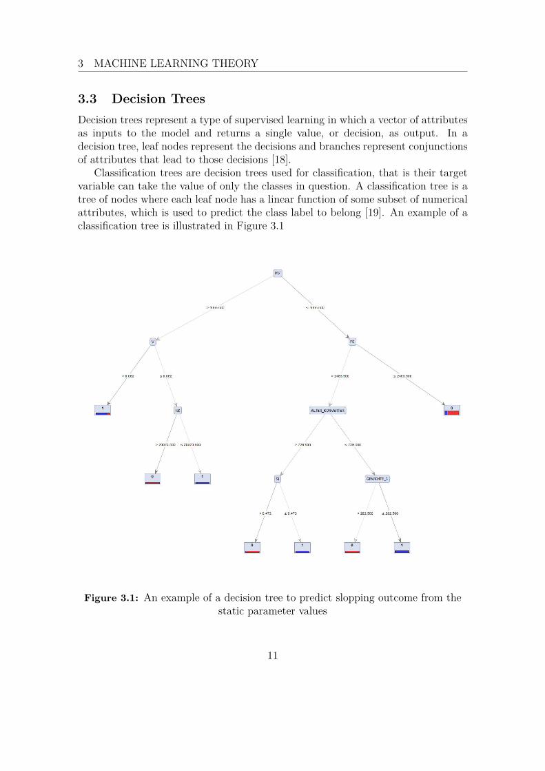
3.3 Decision TreesDecision trees represent a type of supervised learning in which a vector of attributesas inputs to the model and returns a single value, or decision, as output. In adecision tree, leaf nodes represent the decisions and branches represent conjunctionsof attributes that lead to those decisions [18].

Classification trees are decision trees used for classification, that is their targetvariable can take the value of only the classes in question. A classification tree is atree of nodes where each leaf node has a linear function of some subset of numericalattributes, which is used to predict the class label to belong [19]. An example of aclassification tree is illustrated in Figure 3.1

Figure 3.1: An example of a decision tree to predict slopping outcome from thestatic parameter values

11


. The order in which to place the nodes and which node to choose as the rootis decided by examining the entropy and information gain of the attributes. In-formation gain is "the expected reduction of entropy achieved after eliminating anattribute from the equation [19]."

3.4 Random ForestA random forest for classification is an ensemble learning method where severalclassification trees are trained and the mean prediction of the individual trees isthe output. Random forests use a modified tree learning algorithm that selectsa random subset of the attributes at each candidate split in the learning process.Random forests are used to correct for the tendency of decision trees to overfit totraining data [20].

Random forest uses two parameters for tuning a model fit. They are the maxi-mum number of features and the number of estimators. The maximum number offeatures defines how many features to use in each tree and the number of estimatorsdefine how many trees to train in total. The default maximum number of featuresis usually set to the square root of the total number of features and the numberof estimators is usually selected to be as high as possible while keeping trainingtime reasonably short. In order to find optimal parameter settings, these values,are iterated, to fit a final model to the data and the RMSE of the fitted Model isevaluated. The model with the most optimized RMSE value is then selected [18].

3.5 Single Layer Neural NetworkArtificial Neural Networks (ANNs) are modeled according to the biological neuralnetworks that constitute animal brains. Such systems learn to do tasks by consid-ering examples, generally without task-specific programming.

3.5.1 Artificial Neurons

The computing units that are part of a neural network are called artificial neuronsor for short just neurons [21]. The block diagram of Figure 3.2 shows a model of anartificial neuron. The neural model is composed of the following building blocks:

• A set of signals, each characterized by a weight. A signal xj at the input ofsynapse is connected to neuron k is multiplied by the weight ω.

• An adder for summing the input signals, weighted by the respective weights

• An activation function for limiting the amplitude of the output of a neuron.

12


Figure 3.2: Nonlinear model of a neuron

In the neural model presented in Figure 3.2 a bias, b, is applied to the network.The effect of the bias is to decrease or increase the net input of the activation functiondepending on whether it is negative or positive. A mathematical representation ofthe neural network in Figure 3.2 is given by the equations 3 and 4:

v =m∑j=0

ωjxj (3)

y = ψ(v) (4)

where x1, x2,..., xm are the input signals and ω1, ω2,...., ωm are the respectivesynaptic weights of neuron k. The output of the neuron is y represents the lin-ear combiner output due to the input signals. The bias is denoted by b, and theactivation function by ψ.

3.5.2 Single-Layer Feedforward Networks

In the single-layer network there is an input layer of source nodes which direct dataonto an output layer of neurons [21]. This is the definition of a feedforward networkwhere data goes from the input to the output layer but not the other way around.Figure 3.3 shows a single-layer feedforward network.

13


Figure 3.3: Single-Layer Feedforward Network

3.6 The PerceptronThe perceptron is more or less similar to the neuron. The activation function ψ(),acts as a hard limiter, which then produces an output equal to +1 if the hard limiterinput is positive, and -1 if it is negative. In this way, the perceptron can act like aclassifier.

For the perceptron to function properly, the two classes C1 and C2 must belinearly separable. This means that the two patterns to be classified must be suf-ficiently separated from each other to ensure that the decision surface consists of ahyperplane. An example of linearly separable and non separable patterns, in thetwo-dimensional case, is shown in Figure 3.4 [21].

(a) (b)

Figure 3.4: Figure a) showing separable patterns, where the two regions can beseparated by a linear function, while, in Figure b), such separation is not possible

14


Figure 3.5: Multilayer Feedforward Network

3.7 Multilayer Neural networksMultilayer networks are different from single-layer feedforward networks in one re-spect [22]. The multilayer network has one or more hidden layers, whose compu-tation nodes are called hidden neurons. The term ’hidden’ is used because thoselayers are not seen from either the input or the output layers. The task of thesehidden layers is to be part of the analysis of data flowing between the input andoutput layers. By adding one or more hidden layers the network can be capable ofextracting higher order statistics from its input.

The input signal is passed through the first hidden layer for computation. Theresulting signal is then an input signal to the next hidden layer. This procedurecontinues if there are many hidden layers until the signal reaches the output layer,in which case it is considered to be the total response of the network. Figure 3.5shows an example of a multilayer feedforward network with m input units, n hiddenunits and p output units [21].

3.7.1 The Multilayer Perceptron

The Multilayer Perceptron (MLP) consist of neurons whose activation functions aredifferentiable [22]. The network consists of one or more hidden layers and have ahigh degree of connectivity which is determined by weights.

The function signal is the output of a neuron in a preceding layer in the direc-tion from input to output. These signals are then passed to other neurons whichreceive them as input. The error signal comes at the output units and is propagatedbackward layer by layer. Each hidden or output neuron of the multilayer perceptronperform the following computations

1. Computation of the function signal appearing at the output of each neuron,

15


2. Estimation of the gradient vector, which is used in the backward pass throughthe network.

The hidden neurons act as feature detectors, as the learning process progresses,the hidden neurons discover new features in the training data. The hidden unitsperform a nonlinear transformation on the input data into a new space, called thefeature space. In the feature space, the classes of interest in a pattern classificationproblem, may be more easily classified than it would be in the original input space[21].

3.8 Deep LearningDeep Learning provides more stability, generalization, and scalability with big data[1].

Similarly as in Multilayer perceptrons, Deep Learning or Deep Neural networksare Multi-layer, feedforward neural networks, consisting of many layers of inter-connected neuron units, starting with an input layer to match the feature space,followed by multiple layers of nonlinearity, and ending with a classification layer tomatch the output space. The inputs and outputs of the model’s units follow thebasic logic of the single neuron.

As explained in [1], bias units are included in each non-output layer of the net-work. The weights linking neurons and biases with other neurons fully determinethe output of the entire network. Learning occurs when these weights are adaptedto minimize the error on the labeled training data. More specially, for each trainingexample j, the objective is to minimize a loss function, L(W,B | j).

Here, W is the collection (Wi)1:N-1, where Wi denotes the weight matrix con-necting layers i and i + 1 for a network of N layers. Similarly B is the collection(bi)1:N-1, where bi denotes the column vector of biases for layer i + 1.

This basic framework of multi-layer neural networks can be used to accomplishDeep Learning tasks. Deep Learning architectures are models of hierarchical featureextraction, typically involving multiple levels of nonlinearity.

3.8.1 Activation and Loss Functions

The choices for the nonlinear activation function, ψ, are summarized in Table 1below. xi and ωi represent the ring neuron’s input values and their weights, respec-tively.

The distribution functions for the response variable can be specified by using oneof the distribution arguments, like AUTO, Bernoulli, Multinomial, Poisson, etc.

In Table 2, t(j) and o(j) are the predicted (also known as target) output and actualoutput, respectively, for training example j; and y represents the output units andO the output layer.

16


Table 1: Activation functions for the deep learning methods [1]

Function Formula Range

Tanh ψ(v) = ev − e−v

ev + e−vψε[−1, 1]

Rectified Linear ψ(v) = max(0, v) ψεR+Maxout ψ(v1, v2) = max(v1, v2) ψεR

Table 2: Loss functions for the deep learning methods [1]

Function Formula Typical Use

Mean SquaredError

L(W,B|j) = 12 ||t

(j) − o(j)||22 Regression

Absolute L(W,B|j) = 12 ||t

(j) − o(j)||1 RegressionCross Entropy L(W,B|j) =

−∑yεO(ln(o(j)

y ).t(j)y + ln(1− o(j)y )(1− t(j)y ))

Classification

3.8.2 Regularization

Deep Learning framework supports regularization techniques to prevent overfitting.l1(L1: Lasso) and l2(L2: Ridge) regularization enforce modifying the loss functionso as to minimize loss according to the Equation 5:

L′(W,B|j) = L(W,B|j) + λ1R1(W,B|j) + λ2R2(W,B|j) (5)

For l1 regularization, λ1R1(W,B|j) is the sum of all l1 norms for the weightsand biases in the network; l2 regularization via λ2R2(W,B|j) represents the sum ofsquares of all the weights and biases in the network. The constants 1 and 2 aregenerally specified as very small (for example 10−5).

The second type of regularization available for Deep Learning is a modern inno-vation called dropout [23]. Dropout constrains the online optimization such that thenetwork weight values are scaled toward 0. Each training example trains a differentmodel. As a result, dropout allows an exponentially large number of models to beaveraged as an ensemble to help prevent overfitting and improve generalization.

17

4 IMPLEMENTATION

4 | Implementationin this chapter, the detection of the occurrence of slopping using a slop detectionsystem has been described.

4.1 Design of Optical Measuring SystemAs mentioned previously, one of the prevalent techniques for slopping is using directobservations with a camera. In [24] and [25], a slop detection algorithm based onimages from camera’s viewing the tap-hole, has been delineated. In this chaptera slop detection algorithm is presented, which builds on the previously mentionedmethod and is based on camera images taken with a camera viewing the lateral outerwall of the converter, instead of just focusing on the converter mouth. The acquiredimage of the converter mouth is then analyzed using image processing techniques todetect the occurrence of slopping.

4.1.1 Experimental setup

The Camera system was installed in the plant at Salzgitter Steelworks AG. AnFCMOS camera (Figure 4.1) is aimed at the lateral outer wall of the converter, toget a better view of the overflowing slag.

Figure 4.1: Optical measuring system: network-capable camera for the digitaldetection of slopping at the converter mouth.

18

4 IMPLEMENTATION

In Figure 4.2 the experimental set-up is shown. From this position the camerahas a clear view of the converter wall as well as the converter mouth. The imagesare acquired and recorded at a rate of 2.5 frames per second with software designedin OpenCV, using a shutterspeed of 5[ms] and a resolution of 480x640. Figure 4.3shows the images of slopping captured by the camera system.

Figure 4.2: Experimental setup of camera system to detect slopping occurrence atthe BOF converter

19

4 IMPLEMENTATION

Figure 4.3: Images of slopping captured by the camera system

4.1.2 Video Processing Algorithm

The basis for the image processing algorithm is the extraction of light pixels inthe captured image like the bright pixels in the processed image, colored in red(Figure 4.4). The image area for recognition which is relevant from slopping (areaof interest), is set with a green frame in the original captured image.

In order to extract the bright pixels from the original image, the signals, areconverted to a HSV colourspace. Then channel splitting is performed on both theRGB as well as the HSV versions of the images to filter out only the R (Red) andthe V (Value) channels. Two masks are applied on both channels such that thesignals higher than the set threshold values are filtered. Furthermore, those brightareas, which are only temporarily present (e.g. flying sparks) are not taken intoconsideration. The algorithm used for detecting the bright pixels in the capturedimages are shown below in Figure 4.5.

Figure 4.4: Original image of the converter mouth with sparks and small,adhering slag part at the right edge (right) and Result image with recognized slag

part at the converter (left)

20

4 IMPLEMENTATION

Figure 4.5: Algorithm used for detecting the bright pixels in the captured images

Figure 4.6: Detection of incandescent material from the captured image by thecamera to detect illuminated slag particles

In Figure 4.6, the test tool with activated R and V threshold range can beseen. The threshold ranges were adjusted according to the camera. The followingthresholds were found to be suitable:

• V-threshold: 100-254

21

4 IMPLEMENTATION

• R-threshold: 120-254

In Figure 4.6, the detected glowing areas are visible. The two resultant image fromthe two channels are then combined using logical AND function. The remainingpart of the image is then eroded and resultant part is dilated, to emphasize on theslag portion. This eliminates any wayward sparks that may have been capturedin the monitored area of the image. For perfect detection of slag, only the outercontour of the converter needs to be monitored. This is realized by application of amask, in which, the area to be monitored is displayed in white, and the remainingarea is black (Figure 4.7).

Figure 4.7: Figure on the right is generated by applying the thresholding mask onthe input image on the left on the as captured by the camera system

This mask is then loaded into the test tool to ignore the zone with the contentsof the converter (Figure 4.8).

Figure 4.8: The mask is then applied to ignore the zone with the contents of theconverter

22

4 IMPLEMENTATION

During the blow, often, sparks, from the flame, are captured in the monitoredarea of the image. Despite the ROI, some of the flame sparks still manage to becaptured in the monitored area, during the detection of slag slopping.

In order to prevent the flame sparks to be detected, two methods are used:

1. The area to be monitored is set lower

2. A low-pass filter is used

4.2 Design of Acoustic Measuring SystemIn order to reduce or prevent slag ejection at converters for steel production in theconverter, a system was installed for acoustic tracking and evaluation of the blowingprocess in the converter. The audiometric monitoring on a converter is based on thefact that the sound generated at the blow nozzle of the main lance is influenced byslag formation. The sound intensity is high in the initial phase of oxygen blowingand is dampened with the commencing slag formation, during the silicon oxidation.Normally, as a result of the advancing basal process with the sinking mass producedby the decarburization, a typical sound dampening process results, which can betraced back to the slag formation.

The figure shown in Figure 4.9 red line represents the threshold at which thesystem detects an impending slopping occurrence.The threshold value is dependenton a number of variables, converter geometry, Lance procedure, process engineeringet. and was determined empirically beforehand.

Objective of the acoustic system (Figure 4.10) is the realization of a low-maintenanceacoustic monitoring system on a LD converter process. It consists of a sound mea-surement device and a unit for evaluating the signals, which is based on an industrialPC. This PC has a sound card for recording of data originating from the microphonesfor Sound level measurements, a suitable software system and tools for evaluatingthe Sound measurements and visualize the acoustic signal graphs.

The signal is amplified and digitized. The resulting sound levels are archivedin files for later statistical evaluations and together with a slag status indicator forcontrol purposes.

The sound level measuring device consists mainly of microphones, sound tube,condensation microphones, microphone clamping devices, microphone cables, micro-phone preamplifier and an industrial computer for signal evaluation. Components ofthe measuring system are devices of Digigram [26]. The digitalization of the audiotakes place in Digigram ES8mic microphone preamplifiers, which are arranged ineach case close to the sound source.

The transmission of the digitized audio signal over longer distances in the steel-works is carried out via standard Ethernet (fiber optic cable), The Digigram de-vices are interconnected. The digitized audio signals from the four microphones

23

4 IMPLEMENTATION

Figure 4.9: This figure shows the trajectory of a the sound signal over theduration of a heat, when the level of the sound signal crosses the thresholddemarcated by the red line, it indicates that there is a certain probability of

occurrence of slopping

are then connected to the standard Windows Direct Sound Devices of the DigigramLX6464ES sound card and can be read in LabVIEW using the Windows Sound APIs.The sound levels generated as a result of the evaluation are then visualized on theindustrial computer and transferred to the existing automation system (PLC systemand process computer system) via appropriate hardware and software interfaces.

The sound card is configured so that the audio signals from the microphonesare applied to the ethernet sound channels. These can be accessed directly via theWindows Sound API. The sampling frequency was chosen such that a frequencyresolution of the sound signal of at least 15 Hz is enabled. The total frequencyrange to be mapped should be approximately 30 Hz to 10,000 Hz. In addition tothe reading of the sound card channels, up to 8 process parameters (eg. meltingnumber, oxygen quantity, blowing time, etc.) are read in from the automationsystem via the corresponding interface.

The signals of the sound channels are converted to the frequency range usingFast Fourier Transform. After the Fourier transform, a signal smoothening takesplace, which can be parameterized. The levels in the frequency range are weightedaccording to an A-score. For each sound channel, sound levels are formed in threefrequency ranges, whereby the lower limit can be set for each frequency range. From

24

4 IMPLEMENTATION

Figure 4.10: Overview of the sound monitoring system which includes twomicrophones attached to the top (at 19m height) and base of the converter vessel

the discrete levels of the individual frequency ranges, signals are to be generated,that is, a total of 6 sound levels (2 channels, 3 frequency ranges) are produced forthe time domain. The respective level levels can be set by parameterizable factors.

The processed sound waveform is displayed in the HMI of the system. Figure?? shows how slopping phenomena affect the sound. The Sound trajectory (blue)is at the beginning of the melt typically high and then falls rapidly Once the soundcurve falls below a certain predetermined threshold value, changes their color andan indication for slopping is given. The length of time wherein the threshold valueis relevant, is indicated by the extent of the red line and can be changed. Also, theheight of the threshold value can be changed. The batch whose sound level is shownin right image, had no slopping.

4.3 Design of Vibration Measuring SystemLance vibration for estimation of slag formation is based on the theory of transferof kinetic energy from the slag to a mechanical structure for which the vibration ismeasured (i.e. the oxygen lance). This, mainly horizontal transfer of energy to thelance, results in vibration propagating through the structure.

The vibration signal obtained from a sensor (i.e. accelerometer) placed on thetop part of the oxygen lance, was passed through a narrow band pass filter, with amid-frequency equivalent to the lance natural frequency.

25

4 IMPLEMENTATION

Figure 4.11: Schematic of the vibration measurement installation setup at theBOF converter to detect slopping occurrence

The accelerometer used to measure the vibration patterns was an industrial tri-axial accelerometer. It was attached at the top of the lance, to measure the vibrationof the lance, especially during slopping events (Figure 4.11). The wireless modulewas setup with the ibaPDA [27] software, a data acquisition system, for connectedautomation systems. The vibration data was recorded in the form of .DAT files andanalyzed in the ibaAnalyser software [27].

For analysis, the collected vibration data, stored in a raw format of the mea-surement system, was transformed by Fast Fourier Transformation and stored in adata base for further use. The FFT was calculated by using a moving time windowof a length which ensures an overlapping examination of the signals. However, inthis case, only the vibration patterns of 24 heats were recorded, due to some criticalmalfunction the vibration system.

The frequency data were additionally combined with process data such as slop-

26

4 IMPLEMENTATION

ping grade, sound signals, oxygen and carbon-monoxide rate, etc (Figure 4.12).These variables may influence the vibration measurement and therefore they shouldbe represented in parallel to the spectra.

Figure 4.12: Vibration pattern during a heat, corresponds to the patterns of theoxygen rate, lance height and the number of bright pixels; the area in the green

zone shows an instance where a peak in the vibration pattern is also reflected by acorresponding change in the patterns of the oxygen rate, lance height and the

number of bright pixels

In some cases from the vibration patterns of the heats, a few instances wereanalyzed which seemed to correlate with the slopping occurrences as well with themeasurement patterns of the high pixel values and the acoustic systems.

Even though different tests were performed with varying representations of theslopping behavior, and with different compilations of the data sets to cover con-straints of similar distribution of the slopping events inside the analyzed data sam-ple, the results were not satisfying.

The main problems of this analysis are the low amount of data from the heats,and unknown influences into the lance vibration behavior which may cover vibrationsinduced by occurring slag foaming and slopping. Further extended measurements

27

4 IMPLEMENTATION

to investigate these influences were not carried out because of system malfunctionand very little relation observed with slopping events, from the previous heats.

4.4 System Setup

Figure 4.13: Layout of the system at SZFG Salzgitter

As shown in Figure 4.13, the opto-acoustic slopping recognition system is networkedwith:

• The office network in order to remotely access the computer for configuration,maintenance and backup,

• The PLC network of the converter C for data exchange of the acoustic machinewith a control and S7

28

4 IMPLEMENTATION

• The microphone amplifier via a separate Ethernet connection with a soundcard in the computer.

4.4.1 Installation of microphones and camera

The microphone and camera are integrated with special heat protection plates inthe wall of the doghouse.

Figure 4.14: Microphone attachment outside wall in the north east

• Microphone tube with flange: To protect against dust and heat, the micro-phones are attached to a 2m long pipe, which is fastened by means of a pipeflange at the heat protective plate / the boiler.

• Burn plates microphone in the north east side: For the installation of thedoghouse microphone, a two-plate construction is provided; a "roof panel" toprevent slag splashes and a plate with a passage for the microphone (Figure4.14).

• The microphone is located on the north east side compared to the controlcenter in northwest.

29

4 IMPLEMENTATION

Figure 4.15: Installation of the camera System

4.5 DataThe data from the camera and the acoustic sensors as well as the process variabledata from the plant PLC was collected and stored in the database over a period of4 months, from March to June, 2017.

The data collected was of two types:

1. Static data, consisting of information collected before the start of blowing likelime content, Amount of scrap metal etc.

2. Dynamic data, consisting of the information collected during the blowing of

30

4 IMPLEMENTATION

oxygen, like the sensor data, and other process variables like oxygen content,CO content etc.

The static and dynamic data were collected from approximately 2500 heats dur-ing the 4 months.

4.5.1 Static Data

The static data consists of around 30 process variables, collected from 2500 heats,before the start of the blowing process. The process variables consisted of informa-tion on features available before the start of the heat like, heat number, converternumber, amount of different metals like C, Si, Ti, V, and amounts and types ofdifferent scrap. The slopping intensity of each heat was categorized from a scale of0 to 4, 0 being no slopping, to 4 being the highest. Also included in the data, wasthe slopping duration of each heat.

4.5.2 Dynamic Data

Figure 4.16: Sample dataset consisting of dynamic data of heat numbered 72638as measured on 16.01.2017

31

4 IMPLEMENTATION

The dynamic data from each heat consists of the sound sensor values and high pixelintensity, along with other process variables, collected at every second of the heat.On an average, a heat ran for around 1000 seconds, so the table for a sample heathad around 1000 rows. A sample dataset sheet of the dynamic data is shown inFigure 4.16. Every heat was identified with a slopping rating of 0 to 4, similar tothe static data. Some notable process features of the dynamic dataset:

• Blaszeit: The time in seconds calculated from the start of blowing in oneheat

• Sound intensity: The sound intensity values, ’Sound unten’ and ’Soundoben’, calculated from the two sets of microphones, each set placed over andunder the converter, and with three different frequencies, f1, f2 and f3.

• Helle pixel: Number of pixels of high intensity as calculated from the imageprocessing algorithm

4.5.3 Preparation of Data

Both sets of data had to be modified and corrected in order to remove erroneousvalues and encoding errors. This was accomplished using algorithms and scripts inVBA (Visual Basic Applications) and Java.

The raw data contained erroneous values due to defect sensors or incorrect dataprocessing. This data was identified and replaced automatically by reliable values.While this step can sometimes be handled automatically using simple rules (“discardheats where process value X lies outside two standard deviations around the meanvalue of X” [15]), better results will be achieved if such filter rules are specified (orat least reviewed) by a process specialist.

The dynamic dataset contained 2500 tables, each detailing the values of theprocess variables, calculated during the blowing process. In order to make the datamore coherent and for further statistical calculations, it was imperative to combinedata from all the heats to one single data table.

From the newly formed dataset of the dynamic data, average heat graphs werecomputed for both slopping and non-slopping heats. This was achieved by extractingall the data points corresponding to the slopping category (’MAX INTENSITÄTAUSWURF’) 0, for no slopping, and 4, for heavy slopping. Further the averageprocess variable values were computed for each time-point, in both cases, and thencompiled together to form the sample heats for no slopping and heavy slopping.

32

4 IMPLEMENTATION

Figure 4.17: Acoustic plot depicting sound level variations in an average sloppingheat; the black line shows the heat with no slopping, the red line shows the heat

with liquid slopping and the blue line depicts the heat with solid slopping

Figure 4.18: Plot of bright pixels against time in an average slopping heat; theblack line shows the heat with no slopping, the red line shows the heat with liquid

slopping and the blue line depicts the heat with solid slopping

33

4 IMPLEMENTATION

In Figure 4.17, it can be seen that for an average heat having slopping, theacoustic levels are considerably decreased in comparison to the sound levels in aheat with no sloping. This reinforces the hypothesis stated in Section 4.2, that thesound levels are influenced by slopping behavior, and that the sound levels can beused as a reliable factor for predicting future slopping occurrences.

Similarly, Figure 4.18 shows the range of the pixel intensity throughout a heatwith average slopping and no slopping, as calculated by the Optical Measuringsystem. It can be seen that for slopping heats, the pixel intensity is quite high, ascompared to the average heat with no slopping. All these factors, were taken intoconsideration, while developing a prediction system for Slopping events.

One of the major tasks involved was to compile the Static and the Dynamicdatasets into a single table, where each row corresponds to one ’Blaszeit’ time-pointof a particular heat, with both dynamic as well static information recorded of thattime-point. This was achieved using SQL commands and pandas library in Python.The final dataset consisted of more than 600,000 rows and 55 process variables. Ithas to be kept in mind that Only Data of the first 300 seconds of the heats wereused for modeling, as it is imperative to predict the occurrence of slopping as earlyas possible with respect to the time of blowing oxygen.

4.6 Modeling4.6.1 Selection of features

One of the most important steps before training a model is to specify which featuresshall be taken into account as input data of the model. There are two main aspectsto keep in mind here:

First, selecting too many features increases the risk of over-fitting, i.e. the modelbecomes complex and is allowed to adapt to the smallest particularities in the train-ing data, as explained in [15]. Such a model will usually not generalize well, meansthe performance on new data will deteriorate. One of the most general and popu-lar methods to counteract over-fitting is to use cross-validation. As an alternative,some machine learning algorithms, such as Bayesian linear regression [28] or Gaus-sian processes [29], have such complexity control built-in.

The second aspect for feature selection is to avoid inclusion of data which isnot trustworthy, or not available. Although recent sensor technology has becomemore complex and costly, some sensors to measure specific metallurgical featuresare increasingly susceptible and tend to fail. Similar to the data preparation stage,the feature selection was carried out partly manually or automatically.

The manual approach was guided by the process knowledge of a specialist whomade initial decisions about which features seem most likely to have an influence,or which (measured) features are untrustworthy.

34

4 IMPLEMENTATION

The automatic feature selection does not use any information of the process andis normally based on a predefined maximum set of features. The most commonmethods are “Backward elimination” (BE) and “Forward selection” (FS). BE startswith all features and successively removes one feature; FS starts with one feature andadds one feature in each step. These processes automatically evaluate the qualityof the models and stop when the quality (usually measured by cross-validation)does not improve anymore [30]. If information about the process is not available,automatic feature selection will be an excellent way to evaluate the data. However,a major disadvantage faced in this process was the long computing time due to ahigh number of features.

As a result, instead, it was decided to use some algorithms to get an idea, re-garding which of the features exerted the most influence on the Slopping parameter,and to also tell us which of the features to not include while training a model, asthey were either constant, or erroneous. The three algorithms implemented in thisstep were:

1. Select K Best: As defined in the Scikit-learn module documentation [31],"SelectKBest selects the top k features that have maximum relevance with thetarget variable. It takes two parameters as input arguments, "k" (obviously)and the score function to rate the relevance of every feature with the targetvariable."

2. Randomized Lasso: The Scikit-learn module documentation [31] definesthat "Lasso regression performs L1 regularization, i.e. it adds a factor ofsum of absolute value of coefficients in the optimization objective. For Lassoregression, the objective for optimizing the regression, isObjective = RSS + α * (sum of absolute value of regression coefficients), whereRSS stands for ‘Residual Sum of Squares’ which is the sum of square of errorsbetween the predicted and actual values in the training data set."

i a = 0: Same coefficients as simple linear regressionii α = ∞: All coefficients zero (same logic as before)iii 0 < α < ∞: coefficients between 0 and that of simple linear regression

Randomized Lasso works by subsampling the training data and computing aLasso estimate where the penalty of a random subset of coefficients has beenscaled. By performing this double randomization several times, the methodassigns high scores to features that are repeatedly selected across randomiza-tions.

35

4 IMPLEMENTATION

3. Bayesian Regression with Automatic Relevance Determination (ARD)[28]: According to the Scikit-learn module documentation [31], Bayesian Re-gression with Automatic Relevance Determination (ARD) includes "Fit theweights of a regression model, using an ARD prior. The weights of the regres-sion model are assumed to be in Gaussian distributions. Bayesian regressiontechniques can be used to include regularization parameters in the estimationprocedure: the regularization parameter (α) is not set in a hard sense buttuned to the data at hand."

All three of these algorithms were applied on the data, using Python modules,to find out the top influencing features on the slopping factor. The main purposeof these algorithms was to select the set of features that is optimal for building aprediction model from the given data base. At the end, those features which wereeither constant, or had little to no influence on the final model were rejected andthe final set of features were selected for building the model. Figure 4.19 shows therelative importances of the parameters as calculated from the algorithms.

Figure 4.19: Chart of Importance Ratings of the Variables, as calculated using acombination of the ’Select K Best’, ’Randomized Lasso’, and ’Bayesian Regression

with ARD’, applied on all 2500 heats collected from March to June

36

5 RESULTS AND ANALYSIS

5 | Results and AnalysisBefore building the different models the data is divided into training, validationand test data sets. The training set is used to train the different models and thevalidation test is used to verify and evaluate the models during iterative trainingin order to select the best meta parameters. Once the meta parameters have beenchosen and a finished model selected the final model is tested on the test data toevaluate its performance.

The division is done by partitioning the data using a stratified splitting method(Stratified Shuffle Split [31]). The validation and test data sets are also split basedon stratified partitioning. Partitioning using a stratified method ensures that thereis no strong correlation or dependencies between the data in the different sets, asit is made certain that the ’Slopping’ parameter values are uniformly distributed inall the three sets. If a random sampling method had been applied there would be arisk that observations with nonuniform distribution would appear in both trainingand test sets, giving a strong correlation between the data sets.

If stratified splitting method was not used, it could lead to high correlationbetween the data sets. This in turn could potentially lead to overfitting. Partitioningin this way gives a split of 67% training data, 11% validation data and 22% testdata. Since the validation data can be thought of as part of the training data themajor split into training and test sets is approximately 80% to 20%.

5.1 Decision TreeDecision trees are a non-parametric supervised learning method used for classifica-tion and regression. The goal is to create a model that predicts the value of a targetvariable by learning simple decision rules inferred from the data features. For theimplementation of decision trees on the training data set, the DecisionTreeClassifiermodule of the Scikit-learn machine learning library in Python [31] was used. Aswith other classifiers, DecisionTreeClassifier takes as input two arrays: an array X,sparse or dense, of size [n_samples, n_features] holding the training samples, andan array Y of integer values, size [n_samples], holding the class labels for the train-ing samples. After being fitted, the model was used to predict the class of samplesfrom the test data set. The probability of each class can be predicted, which is thefraction of training samples of the same class in a leaf. The ‘Gini’ impurity functionwas used to measure the quality of split in a node.

After the fitted model was applied on the test data set to evaluate, a MeanSquared Error (MSE) of 0.00021 was recorded. To verify the authenticity of the fittedmodel, a method known as cross-validation was used to further evaluate the fittedmodel. By definition [32], [33], "Cross-validation, is a model validation technique for

37


assessing how the results of a statistical analysis will generalize to an independentdata set. It is mainly used in settings where the goal is prediction, and one wantsto estimate how accurately a predictive model will perform in practice. The goal ofcross-validation is to define a validation dataset to "test" the model in the trainingphase, in order to limit problems like overfitting, give an insight on how the modelwill generalize to an independent dataset (i.e., an unknown dataset, for instancefrom a real problem), etc. "

One round of cross-validation involves partitioning a sample of data into com-plementary subsets, performing the analysis on one subset (called the training set),and validating the analysis on the other subset (called the validation set or test-ing set). To reduce variability, multiple rounds of cross-validation are performedusing different partitions, and the validation results are combined (e.g. averaged)over the rounds to estimate a final predictive model. In these cases, a fair wayto properly estimate model prediction performance is to use cross-validation as apowerful general technique.In summary, cross-validation combines (averages) mea-sures of fit (prediction error) to derive a more accurate estimate of model predictionperformance.

A cross-validation of the algorithm was then performed on the whole datasetwith 20 folds. The mean cross-validation score was 0.601. The resulting confusionmatrix is shown in Figure 5.1.

Figure 5.1: Confusion Matrix for implementation of decision tree algorithm topredict slopping occurrence;the slopping categories [0], [1], [2], [3] and [4] are

predicted, with [0] indicating no slopping, and [4] indicating maximum slopping;the vertical rows depict the actual values while the horizontal rows show the

predicted values by the algorithm

38


5.2 Random ForestA random forest fits a number of decision tree classifiers on various sub-samplesof the dataset and use averaging to improve the predictive accuracy and controlover-fitting. For the implementation of Decision trees on the training data set,the RandomForestClassifier module of the Scikit-learn Machine learning library inPython [31] was used. The parameter n_estimators, which defines the number oftrees trained in the ’forest’ was set to 100. All the features in the Training data wasused to train the model. After being fitted, the model was used to predict the classof samples from the test data set and also, the corresponding probabilities. Afterthe fitted model was applied on the test data set to evaluate, a Mean Squared Error(MSE) of 0.00026 was recorded.

A cross-validation of the algorithm was then performed on the whole dataset with10 folds. The mean cross-validation score was 0.70. The resulting cross-validationmatrix is shown in Table 5.1.

Figure 5.2: Confusion Matrix for Implementation of random forest algorithm topredict slopping occurrence;the slopping categories [0], [1], [2], [3] and [4] are



39


For both cases of decision tress and random forests implementations, the test re-sults were very promising, with almost 90% accuracy. However, the cross-Validationresults only yielded around 60% average score in both the cases.This discrepancyin the two validations proved that in both instances, the model was overfitting byconsiderable proportions.

5.3 Deep Learning5.3.1 H2O

H2O, as defined by [34] "is an open source, in-memory, distributed, fast, and scalablemachine learning and predictive analytics platform that allows to build machinelearning models on big data and provides easy productionalization of those models."

The H2O module can be implemented on statistical softwares like R, Python,and other environments. It is used for exploring and analyzing datasets held incloud interfaces as well as, in the conventional operating-systems Linux, MacOS,and Microsoft Windows. The H2O software is written in Java, Python, and R.

Inside H2O, a Distributed Key store is used to access and reference data, models,objects, etc., across all nodes and machines. The algorithms are implemented ontop of H2O’s distributed framework. The data is read in parallel and is distributedacross the cluster and stored in memory in a columnar format in a compressed way.H2O’s data parser supports data intake from multiple sources in various formats[34].

The main advantages of using H2O is the concept of a multi-node cluster withshared memory model, where all computations are performed in memory. Each nodesees only some rows of the data and there is no limit on cluster size. Objects in theH2O cluster such as data frames, models and results are all referenced by key. Anynode in the cluster can access any object in the cluster by key. The data frames aredistributed like a collection of vectors and the columns are distributed across nodes,such that each node must be able to see the entire dataset.

5.3.2 Deep learning in H2O

Deep learning methods use a composition of multiple nonlinear transformations tomodel high-level abstractions in data. Deep learning with H2O features automaticadaptive weight initialization, automatic data standardization, expansion of categor-ical data, automatic handling of missing values, automatic adaptive learning rates,various regularization techniques, automatic performance tuning, load balancing,grid-search, N-fold cross-validation, checkpointing, and different distributed train-ing modes on clusters for large data sets. There is no complicated configuration filesand H2O deep learning is highly optimized for maximum performance [1].

40


As mentioned in Section 3.8.1, the process of minimizing the loss function L(W,B| j) is accomplished using a parallelized version of Stochastic Gradient Descent(SGD), in H2O. In standard standard SGD as mentioned by [35], the gradient∇L(W,B|j) is computed via backpropagation .

Although stochastic gradient descent is fast and memory-efficient, to make itfaster, Hogwild!, a recently developed lock-free parallelization scheme from [36] hasbeen used, which follows a shared memory model where multiple cores (where eachcore handles separate subsets or all of the training data) are able to make inde-pendent contributions to the gradient updates ∇L(W,B|j) asynchronously. In amulti-node system, this parallelization scheme works on top of H2O’s distributedsetup that distributes the training data across the cluster. Each node operates inparallel on its local data until the final parameters W,B are obtained by averaging.

Parallel distributed and multi-threaded training with SGD in H2O deeplearning

1. Initialize global model parameters W,B

2. Distribute training data across nodes

3. Iterate until convergence criterion reached:

(A) For nodes n with training subset τn, partition the active subsets by num-ber of cores

(B) Update all sets of W,B(C) Optionally score the model(D) train/validation scoring sets

An H2O cluster was setup for running the deep learning algorithm in Python.The details of the cluster setup is provided in Table 3.

H2O supports model tuning in grid search by allowing users to specify sets ofvalues for parameter arguments and observe changes in model behavior. In the Rand Python examples below, three different network topologies and two different l1norm weights are specified. This grid search model trains six different models usingall possible combinations of these parameters; other parameter combinations can bespecified for a larger space of models.

Grid search provides more subtle insights into the model tuning and selectionprocess by inspecting and comparing the trained models after the grid search processis complete. Grid search parameters used for tuning the model hyperparameters in-volve, the number of hidden layers, ’hidden_opt = [[30, 30, 30], [40, 40, 40], [50, 50, 50]]’

41


Table 3: Features of H2O cluster that was setup for building the predictive model

H2O cluster uptime 06 secsH2O cluster version 3.10.4.8

H2O cluster version age 3 months and 10 daysH2O cluster name H2O_from_python_GHBI_mn4iji

H2O cluster total nodes 1H2O cluster free memory 1.778 GbH2O cluster total cores 8H2O cluster allowed core 8

H2O cluster status accepting new members, healthyH2O connection url http://127.0.0.1:54321

H2O connection proxy -H2O internal security False

Python version 3.6.0 final

and the l_1 norm weights as ’l_1_opt = [1e− 4, 1e− 3, 1e− 5]’. The results of thegrid search is shown on Figure 5.3

Figure 5.3: Table showing a plot of the variation of the mean squared error(MSE) for different number of hidden nodes, in the H2O deep learning model,

calculated using the training dataset

42


From Figure 5.3, it can be seen that the Mean Squared Error is least in case of adeep neural network with 3 hidden layers, each with 50 nodes, and with a l_1 normweight of 1e-5.

The deep learning algorithm was then applied, with the hidden layers and normweight combination, on the training data set to build a model. The new model wasthen tested on test data set and results are shown in Tables 4, 5 and 6.

Table 4: Results of application of deep learning model on test data, showing themean squared error (MSE), the root mean squared error (RMSE), the logloss of

the model and the mean error per class

MSE 0.088RMSE 0.297LogLoss 0.27

Mean Per-Class Error 0.298

Table 5: Confusion matrix for implementation of deep learning algorithm topredict slopping occurrence;the slopping categories [0], [1], [2], [3] and [4] are



0 1 2 3 4 Error Rate (number of wrongpredictions/total number ofpredictions)

79003 0 1345 467 1198 0.037 3,010 / 82,013123 0 322 299 187 1 931 / 931878 0 7969 159 168 0.131 1,205 / 9,174546 0 412 7052 330 0.154 1,288 / 8,3402878 0 1277 438 22643 0.169 4,593 / 27,23683428 0 11325 8415 24526 0.086 11,027 / 127,694

43


Table 6: Table showing the full scoring history of the H2O deep learningalgorithm on the test data which includes the duration per iteration, the trainingspeed of the model, the number of predictions made and the classification error

Duration Training Speed Epochs Iterations RMSE ClassificationError

4.11 sec 43424 obs/sec 0.26 1 0.52 0.314.324 sec 58452 obs/sec 1.82 7 0.46 0.2620.76 sec 61590 obs/sec 2.87 11 0.41 0.21

... ... ... ... ... ...2 min 24.809 sec 77306 obs/sec 26.3 101 0.31 0.112 min 25.317 sec 77302 obs/sec 26.3 101 0.27 0.09

From the results shown in the above tables, it can be inferred that the deeplearning algorithm has performed more or less similarly compared to decision treeand random forest, when tested on the same test data set.

For this reason, this same algorithm was then applied on the validation data setusing cross-validation of 5 folds. The results of the cross-validation implementationare shown in Tables 7, 8 and 9.

Table 7: Results of application of deep learning model using cross-validation,showing the mean squared error (MSE), the root mean squared error (RMSE), the

logloss of the model and the mean error per class

MSE 0.068RMSE 0.26LogLoss 0.22

Mean Per-Class Error 0.3

44


Table 8: Confusion matrix for implementation of deep learning algorithm, usingcross-validation, to predict slopping occurrence;the slopping categories [0], [1], [2],

[3] and [4] are predicted, with [0] indicating no slopping, and [4] indicatingmaximum slopping; the vertical rows depict the actual values while the horizontal

rows show the predicted values by the algorithm

0 1 2 3 4 Error Rate399367 0 2942 1404 6145 0.025 310,491 / 409,8581310 2 2458 613 429 0.999 4,810 / 4,8127552 0 34262 2027 2255 0.256 11,834 / 46,0963927 0 699 35012 2085 0.16 6,711 / 41,7236816 0 982 3551 125587 0.082 11,349 / 136,936418972 2 41343 42607 136501 0.07 45,195 / 639,425

Table 9: Metrics Summary for the deep learning model after cross-validation

Metrics Mean StandardDeviation

Fold1

Fold2

Fold3

Fold4

Fold5

Accuracy 0.93 0.005 0.93 0.94 0.93 0.93 0.91Mean Accuracy

per Class0.7 0.02 0.71 0.71 0.72 0.69 0.64

Mean Error perClass

0.3 0.02 0.29 0.28 0.28 0.3 0.35

Mean SquaredError

0.06 0.006 0.06 0.056 0.062 0.07 0.08

R2 0.98 0.002 0.98 0.98 0.97 0.97 0.97

5.4 Final Comparison of ModelsFigure 5.4 illustrates the accuracy distribution of the cross-validation metrics ofthree models, decision trees, random forests and deep learning. It can be seenthat the deep learning algorithm has the minimum variance over the range of thecross-validation iterations, which means that the all models in the cross-validationcalculations give more or less a similar performance, irrespective of the Training andValidation sets, compared to the other two algorithms, in terms of prediction. Inother words, the deep learning algorithm can be said to be generalizing very well,

45


and the chances of overfitting is reduced to the bare minimum. Based on thesefactors, a decision was taken to implement the deep learning algorithm for furthertesting.

Figure 5.4: Comparison of variance of accuracy distribution of cross-validationmetrics of three models, decision trees, random forests and deep learning

5.5 Implementation of model in server for online testingThe final step in testing the model was to deploy it online on a server. This wasneed to be done in order to test how the model performed when executed online andto build a prototype of a system in which it was possible to perform prediction andanalysis automatically on the server.

The tools used to achieve this goal were Rapidminer Studio and RapidminerServer. RapidMiner [37] "is a data science software platform developed by the com-pany of the same name that provides an integrated environment for data preparation,machine learning, deep learning, text mining, and predictive analytics." RapidMineruses a client/server model with the server offered as on-premise, or in public orprivate cloud infrastructures. RapidMiner is written in the Java programming lan-guage. RapidMiner provides a GUI to design and execute analytical workflows.

46


RapidMiner provides learning schemes, models and algorithms and can be extendedusing R and Python scripts.

RapidMiner Server [37] is a performance-optimized application server, it is pos-sible to schedule and run analytic processes and quickly return results. It seamlesslyintegrates with not only RapidMiner Studio, allowing processes to continually up-date so that they reflect any changes to external data sources. It is possible to —locally or remotely — collaborate, build, and visualize results using charts and maps,online. There are several main components to a RapidMiner Server configuration:

• RapidMiner Studio: RapidMiner Studio and RapidMiner Server connectand interact with each other, employing standard protocols.

• RapidMiner Server

• RapidMiner Server repository: The RapidMiner Server repository con-tains the RapidMiner Server processes and data.

• Data sources: The user data sources used for model building. Connectionsallow to connect to databases or to connect to other data sources.

• Operations database: It is possible to use an existing database server orcreate a new one; it can reside locally or on a remote host.

The Rapdiminer Server architecture is shown in Figure 5.5

Figure 5.5: Rapidminer Studio and Rapidminer Server Architecture

RapidMiner Studio and RapidMiner Server communicate via HTTP(S); Thecommunication port must be assigned and opened on each instance in the configu-ration. The developed Deep Learning model for the detection of slopping was then

47


implemented in the Rapidminer Server for onsite testing. The model was first re-alized in the Rapidminer Studio software and then, the model was uploaded intothe server. The server API was then used to develop a Human Machine Interface(HMI), which was utilized to enter each set of readings from the sensors. The modelwas then executed and the predictions, along with the confidence measures for eachcategory, was displayed online. A graph, depicting confidence measures for consec-utive sets of readings, was also displayed. Figure 5.6 shows the screenshot of theGraphical User Interface, of the application developed.

Figure 5.6: Graphical User Interface for online execution of Predictive Model forSlopping Detection

48

6 CONCLUSIONS AND DISCUSSION

6 | Conclusions and DiscussionInferring from the results and analysis of the entire project, it can be concludedthat Slopping detection was successful to a great extent. Although the system wasnot tested in real plant conditions, still early results from partial and offline testslook promising. A study of the slopping videos, captured by the camera system, inthe plant have given an idea of a basic pattern for slopping heats. In most cases ofslopping, usually, for heats with some extent of slopping occurrences, there was aconsiderable probability that slopping will also take place in the next few heats aswell.

Both the studies of the number of high pixels from the image analysis as well asthe trajectories of the acoustic signal curves, correlate to the slopping phenomenon.This re-affirms the hypothesis that the sound levels go down during slopping becauseof the slag emulsion muffling the sound from the converter vessel.

Although the analysis of the vibration measurement system proved inconclusive,it still showed signs of promise. From the limited number of vibration data available,it was still managed to form some correlation and patterns with the slopping factors.It may be possible to do an in-depth research into the vibration pattern analysis, ifthe system executes without malfunction, and more data can be available. In sucha case, it will be interesting to see how this vibration pattern data correlates toslopping, and to what extent can the prediction model be improved by the inclusionof that data.

The initial offline analysis of the static and the dynamic data proved successful.A test was conducted in the plant with only the static test available. Althoughthese results looked promising, it was still inconclusive as the data was unreliableto a certain extent. However, future on site tests with both the dynamic as well asthe static process data may prove to be fruitful.

The offline tests re-iterate the hypothesis that for highly accurate predictions ofslopping, the Deep Learning algorithm stood out among the rest. Both the DecisionTrees as well as the Random Forests algorithms did not generalize well, and wereprone to overfitting. Other algorithms like K-Nearest Neighbors (KNN) and SupportVector Machines (SVM) were also tested but, did not prove effective, either becauseof limited accuracy or due to highly intensive and time-consuming computations.

The application of the machine learning platform H2O was very effective, for theimplementation of the Deep Learning Algorithm. The cluster system of the H2Oplatform helped in decreasing much of the computational intensity as well as thetraining time. The Deep Learning algorithm performed better than many of theother Machine Learning models, in terms of both accuracy as well as performanceintensity. Given the positive results, the H2O platform may be used in the futurefor further predictive modeling in BOF Converter applications.

49


On comparison with the existing state-of-the-art systems on slopping detection,this system incorporates both static and dynamic process variables as well as datareceived from the image processing and acoustic devices. Till now, it is difficult tofind a single slopping prediction system which employs all the above characteristicsall in one. [3] introduces the image processing technique but does not involve anymachine learning models, only linear statistical models. [11] employs the Imageprocessing, Sound processing as well as vibration analysis, but the discussion in thepaper is only qualitative and does not involve any prediction system or machinelearning model. The papers [15] and [16] introduce the principle of creating a datadriven prediction model, but it is for end-point prediction, and not for slopping.The projects discussed in the BATHFOAM [12] are the some of the limited numberof projects to involve machine learning models together with sensor fusion systems.However, as explained in Section 2.4, none of the projects involve all the three sensorsystems, viz. Image processing, Acoustic monitoring and Vibratory signal analysistogether. Also, the use of Deep Learning methods for accurate prediction of sloppingoccurrences is quite unique, in comparison to the other systems discussed so far. InTable 10, the developed opto-acoustic system has been compared with the existingmethods.

50


Table 10: Comparison of the developed system with the existing methods

Projects ImageProcessing

AcousticProcessing

VibrationPatternAnalysis

PlantrelatedProcessvariables

MachineLearningAlgorithm

used

Purpose

Thesis byC.

Kattenbelt[3]

X - - X - Slopping

IMPHOSproject[11]

X X X - - PhosphorousContentmeasurement

End PointPrediction[15],[16]

- - - X BayesianLinearModels,SupportVectorMachine(SVM)

BOF End-Point Predic-tion

Tata SteelScun-thorpe[12]

- X - X SOM,MLP,

DecisionTrees

Slopping

ArcelorMittal

Gent [12]

- - - X MLP,DecisionTrees

Slopping

ArcelorMittalMaiziers

[12]

- - - X NeuralNetworks

Slopping

ArcelorMittal

Spain [12]

- X X X PCA,MARS,CHAIDDecisionTrees

Slopping

Opto-AcousticSystems

X X X X DeepLearningAlgorithm

Slopping

51


Future WorkThe study conducted in this thesis project was an initial research and estimation togauge the performance of data driven models for prediction of Slopping and otherphenomena related to the BOF Converter Process. The promising results of thisresearch should provide further incentive to improve and fine-tune this system forfuture production. The future scope for this project is quite large and some of thepotential advancements in this system in the future are mentioned below:

• There is scope for improvement of the database system for automatic andonline storing of the process datasets, such that the data can be ready formodeling and prediction in real time.

• The sensor system connections must be upgraded to improved network tech-nologies like cloud for fast processing of the signals along with the plant PLC.

• An improved HMI system will prove effective for visualization of the sensorsignals as well as the process parameters. The HMI, designed in Labview,will be used to integrate the predictive model, which will be able to run inparallel with the HMI system, thus giving predictions in real time, based onthe incoming data.

• Further tests are needed to be performed inside the plant in real plant condi-tions to estimate the performance of the entire sensor and prediction systemin real time. Based on the tests, further changes and improvements are neededto be made on the prediction model, wherever applicable.

• Implement a sliding model system which continues to update itself with recenttraining data at a regular interval.

52

REFERENCES

References[1] A. Candel, E. LeDell, V. Parmar, and A. Arora, “Deep Learning with H2o,”

Aug. 2017. [Online]. Available: http://docs.h2o.ai/h2o/latest-stable/h2o-docs/booklets/DeepLearningBooklet.pdf

[2] “McKinsey-Studie zu Industrie 4.0: Deutsche Un-ternehmen trotz wachsender Konkurrenz zuversichtlich |mckinsey.de.” [Online]. Available: https://www.mckinsey.de/mckinsey-studie-zu-industrie-40-deutsche-unternehmen-trotz-wachsender-konkurrenz-zuversichtlich

[3] C. Kattenbelt, “Modeling and optimization of slopping pre-vention and batch time reduction in basic oxygen steelmak-ing,” Ph.D. dissertation, University of Twente, Enschede, Jul.2008. [Online]. Available: https://research.utwente.nl/en/publications/modeling-and-optimization-of-slopping-prevention-and-batch-time-r

[4] M. Brämming, “Avoiding slopping in top-blown BOS vessels,” LicentiateThesis, uleå University of Technology, Department of Civil, Environmentaland Natural Resources Engineering, Sustainable Process Engineering,2010. [Online]. Available: http://www.diva-portal.org/smash/record.jsf?aq2=%5B%5B%5D%5D&c=1&af=%5B%5D&searchType=SIMPLE&query=Avoiding+slopping+in+top-blown+BOS+vessels&language=en&pid=diva2%3A990331&aq=%5B%5B%5D%5D&sf=all&aqe=%5B%5D&sortOrder=author_sort_asc&onlyFullText=false&noOfRows=50&dswid=-2942

[5] R. J. Fruehan and A. S. Foundation, The Making, Shaping, and Treating ofSteel: Steelmaking and refining volume. AISE Steel Foundation, 1998, google-Books-ID: dZ_ORwAACAAJ.

[6] D. Webster, K. Greenhalgh, and C. Boswell, “Recent Development in ProcessControl and Efficiency at BHP Newcastle Works BOS Shop,” in Proc. 68th ISSSteelmaking Conf., vol. 68, Detroit, Michigan, USA, 1985, pp. 299–307.

[7] C. Bencini and A. Poli, “Automation for refining and slag control in LD processat AFP/ Piombino steel shop,” Dallas, 1993, pp. 193–198.

[8] T. Kanai, A. Sakai, J. Tani, S. Yoshida, and N. Matsui, “Development of aslopping prediction and control system in BOF operation,” Toronto, 1997, pp.267–275.

53

http://docs.h2o.ai/h2o/latest-stable/h2o-docs/booklets/DeepLearningBooklet.pdf

http://docs.h2o.ai/h2o/latest-stable/h2o-docs/booklets/DeepLearningBooklet.pdf

https://www.mckinsey.de/mckinsey-studie-zu-industrie-40-deutsche-unternehmen-trotz-wachsender-kon kurrenz-zuversichtlich

https://www.mckinsey.de/mckinsey-studie-zu-industrie-40-deutsche-unternehmen-trotz-wachsender-kon kurrenz-zuversichtlich

https://research.utwente.nl/en/publications/modeling-and-optimization-of-slopping-prevention-and-batch-time-r

https://research.utwente.nl/en/publications/modeling-and-optimization-of-slopping-prevention-and-batch-time-r

http://www.diva-portal.org/smash/record.jsf?aq2=%5B%5B%5D%5D&c=1&af=%5B%5D&searchType=SIMPLE&query=Avoiding+slopping+in+top-blown+BOS+vessels&language=en&pid=diva2%3A990331&aq=%5B%5B%5D%5D&sf=all&aqe=%5B%5D&sortOrder=author_sort_asc&onlyFullText=false&noOfRows=50&dswid=-2942





REFERENCES

[9] H. Takezoe, T. Saito, K. Ebato, J. Katsuda, M. Azuma, and S. Hato-Guchi,“Some trials in the development of a slopping prediction technique in the BOFat Kakogawa works Kobe Steel Ltd.” 1991, pp. 1368–1370.

[10] M. Evestedt and A. Medvedev, “Model-based Slopping Warning in the LD SteelConverter Process,” Journal of Process Control, vol. No. 19, pp. 1000–1010,2009.

[11] “European Commission : CORDIS : Projects : IMPHOS - Improvingphosphorus refining,” Tech. Rep. 80409, Dec. 2009, project ID: RFSR-CT-2006-00006 Funded under: ECSC-COAL-STEEL-RTD C. [Online]. Available:http://cordis.europa.eu/project/rcn/80409_en.html

[12] P. O. o. t. E. Union, “Control of slag and refining conditions in theBOF (Bathfoam),” Tech. Rep., Oct. 2014, iSSN 1831-9424, ISBN 978-92-79-29232-3, DOI 10.2777/94993, Catalogue number KI-NA-25906-EN-N.[Online]. Available: https://publications.europa.eu/en/publication-detail/-/publication/9c8f4509-b410-4177-a51e-ce0e240ec16f

[13] J. H. Friedman and C. B. Roosen, “An introduction to multivariate adaptiveregression splines,” Statistical Methods in Medical Research, vol. 4, no. 3, pp.197–217, Sep. 1995.

[14] J. N. Luchman, “CHAID: Stata module to conduct chi-square automatedinteraction detection,” Feb. 2015. [Online]. Available: https://ideas.repec.org/c/boc/bocode/s457752.html

[15] S. Klanke, M. Löpke, N. Uebber, H.-J. Odenthal, J. Van Poucke, and A. VanYperen-De Deyne, “Advanced Data-driven Prediction Models for BOF end-point detection,” 2017.

[16] J. Schlüter, H.-J. Odenthal, N. Uebber, H. Blom, and K. Morik, “Reliable BOFendpoint prediction by a real-time data driven model,” Indianapolis (USA),2014, pp. 1–7.

[17] D. Wackerly, W. Mendenhall, and R. L. Scheaffer, Mathematical Statistics withApplications, 7th ed., Cengage Learning, Boston, MA, USA, 2007.

[18] H. Almer, “Machine learning and statistical analysis in fuel consumption pre-diction for heavy vehicles,” Degree Project in Computer Science, KTH RoyalInstitute of Technology, Stockholm, Sweden.

[19] S. Russell and P. Norvig, Artificial Intelligence: A Modern Approach, 3rd ed.Upper Saddle River, NJ, USA: Prentice Hall Press, 2009.

54

http://cordis.europa.eu/project/rcn/80409_en.html

https://publications.europa.eu/en/publication-detail/-/publication/9c8f4509-b410-4177-a51e-ce0e240ec16f

https://publications.europa.eu/en/publication-detail/-/publication/9c8f4509-b410-4177-a51e-ce0e240ec16f

https://ideas.repec.org/c/boc/bocode/s457752.html

https://ideas.repec.org/c/boc/bocode/s457752.html

REFERENCES

[20] L. Breiman, “Random Forests,” Machine Learning, vol. 45, no. 1, pp. 5–32,Oct. 2001. [Online]. Available: https://link.springer.com/article/10.1023/A:1010933404324

[21] G. Batres-Estrada, “Deep learning for multivariate financial time series,”Degree Project in Mathematical Statistics, KTH Royal Institute of Technology,Stockholm, Sweden, 2015, iSRN-KTH/MAT/E–15/40–SE. [Online]. Available:http://www.kth.se/sci

[22] S. O. Haykin, Neural Networks and Learning Machines, 3rd ed. New York:Pearson, Nov. 2008.

[23] G. Hinton, N. Srivastava, A. Krizhevsky, I. Sutskever, and Salakhutdinov,“Improving neural networks by preventing co-adaptation of feature detectors,”Department of Computer Science, University of Toronto, 6 King’s CollegeRd, Toronto, Ontario M5S 3G4, Canada, Tech. Rep., Mar. 2012. [Online].Available: https://arxiv.org/pdf/1207.0580.pdf

[24] H. Iso, K. Arima, M. Kanemoto, Y. Ueda, and H. Yamane, “Prediction andsuppression of slopping in the converter,” Transactions ISIJ, pp. 382–390, 1988.

[25] M. Oda, M. Yoshino, Y. Muraki, and T. Hasegawa, “Development of the slop-ping predictive and suppressing system in LD converter,” Nagoya, 1990, pp.109–114.

[26] “Digigram : Harnessing IP technologies for flexible workflows.” [Online].Available: https://www.digigram.com/

[27] “ibaAnalyzer: iba AG.” [Online]. Available: http://www.iba-ag.com/en/products/software/ibaanalyzer/

[28] M. Tipping, “Sparse Bayesian learning and the relevance vector machine,” Jour-nal of Machine Learning Research, pp. 211–244, 2011.

[29] C. E. Rasmussen and C. Williams, “Gaussian Processes for Machine Learning,”MIT Press, 2006.

[30] I. Guyon and A. Elisseeff, “An Introduction to Variable and Feature Selection,”Journal of Machine Learning Research, pp. 1157–1182, 2003.

[31] P. et al, “Scikit-learn: Machine Learning in Python,” JMLR 12, pp. 2825–2830,2011.

[32] S. Geisser, “Predictive Inference.” New York, NY, USA: Chapman and Hall,1993.

55

https://link.springer.com/article/10.1023/A:1010933404324

https://link.springer.com/article/10.1023/A:1010933404324

http://www.kth.se/sci

https://arxiv.org/pdf/1207.0580.pdf

https://www.digigram.com/

http://www.iba-ag.com/en/products/software/ibaanalyzer/

http://www.iba-ag.com/en/products/software/ibaanalyzer/

REFERENCES

[33] P. A. Devijver and J. Kittler, “Pattern Recognition: A Statistical Approach.”London: Prentice-Hall, 1982.

[34] “H2o.ai.” [Online]. Available: https://www.h2o.ai/

[35] Y. LeCun, L. Bottou, G. Orr, and K. Muller, “Efficient BackProp,” Tech. Rep.,1998. [Online]. Available: http://yann.lecun.com/exdb/publis/pdf/lecun-98b.pdf

[36] F. Niu, B. Recht, C. Re´, and Wright, “HOGWILD!: A Lock-Free Approachto Parallelizing Stochastic Gradient Descent,” Computer Sciences DepartmentUniversity of Wisconsin-Madison, Madison, WI 53706, Tech. Rep., 2011.[Online]. Available: http://i.stanford.edu/hazy/papers/hogwild-nips.pdf

[37] “Data Science Platform.” [Online]. Available: https://rapidminer.com/

56

https://www.h2o.ai/

http://yann.lecun.com/exdb/publis/pdf/lecun-98b.pdf

http://yann.lecun.com/exdb/publis/pdf/lecun-98b.pdf

http://i.stanford.edu/hazy/papers/hogwild-nips.pdf

https://rapidminer.com/

TRITA TRITA-ICT-EX-2017:176

www.kth.se

opto-acoustic slopping prediction system in basic oxygen

Documents