optimum asset availability modeled by q-weibull
TRANSCRIPT

João Luis Reis e Silva
Optimum Asset Availability Modeled by
q-Weibull Distribution and Non-Perfect Repairs
Belo Horizonte – MG
Dezembro de 2017


João Luis Reis e Silva
Optimum Asset Availability Modeled by q-Weibull
Distribution and Non-Perfect Repairs
Dissertação de Mestrado submetida à BancaExaminadora designada pelo Colegiado doPrograma de Pós-Graduação em EngenhariaElétrica da Escola de Engenharia da Universi-dade Federal de Minas Gerais, como requisitopara obtenção do Título de Mestre em Engen-haria Elétrica.
Universidade Federal de Minas Gerais
Escola de Engenharia
Programa de Pós-Graduação em Engenharia Elétrica
Supervisor: Prof. Dr. Rodney Rezende Saldanha
Co-supervisor: Prof. Dr. Adriano Chaves Lisboa
Belo Horizonte – MG
Dezembro de 2017

João Luis Reis e SilvaOptimum Asset Availability Modeled by q-Weibull Distribution and Non-Perfect
Repairs/ João Luis Reis e Silva. – Belo Horizonte – MG, Dezembro de 2017-95 p. : il. color; 30 cm.
Supervisor: Prof. Dr. Rodney Rezende Saldanha
Dissertação (Mestrado) – Universidade Federal de Minas GeraisEscola de EngenhariaPrograma de Pós-Graduação em Engenharia Elétrica, Dezembro de 2017.
1. Optimization. 2. Reliability. 3. Restoration Factors. I. Saldanha, RodneyRezende. II. Universidade Federal de Minas Gerais. III. Escola de Engenharia. IV.Optimum Asset Availability Modeled by q-Weibull Distribution and Non-Perfect Repairs

João Luis Reis e Silva
Optimum Asset Availability Modeled by q-WeibullDistribution and Non-Perfect Repairs
Dissertação de Mestrado submetida à BancaExaminadora designada pelo Colegiado doPrograma de Pós-Graduação em EngenhariaElétrica da Escola de Engenharia da Universi-dade Federal de Minas Gerais, como requisitopara obtenção do Título de Mestre em Engen-haria Elétrica.
Trabalho aprovado. Belo Horizonte – MG, 22 de dezembro de 2017:
Prof. Dr. Rodney Rezende SaldanhaDEE UFMG
Prof. Dr. Adriano Chaves LisboaDiretor Técnico GAIA BHTEC
Prof. Dr. Carlos Andrey MaiaDEE UFMG
Profa. Dra. Alessandra Lopes CarvalhoDepto. Eng. Elétrica PUC-MG
Prof. Dr. Douglas Alexandre Gomes VieiraDiretor Técnico ENACOM BHTEC
Dr. Lucas Sirimarco Moreira GuedesGerência de Planejamento VLI
Belo Horizonte – MGDezembro de 2017


This master thesis is dedicated to the memory of engineer and professor Eduardo de Santana
Seixas, a great colleague and friend who inspired and taught me in all fields of reliability
engineering.


Acknowledgements
I would like to thank and express my sincere gratitude to my advisor Prof. Dr. RodneyRezende Saldanha for the continuous support during the entire period of my master degree,for his motivation, immense enthusiasm, knowledge and to support my study and research inreliability engineering area.
My sincere thanks also to my co-supervisor Prof. Dr. Adriano Chaves Lisboa for hisguidance help in all the time of research papers and writing of this master thesis.
I would like to thank the rest of my master thesis committee: Prof. Dr. Carlos AndreyMaia, Prof. Dr. Douglas Alexandre Gomes Vieira, Profa. Dra. Alessandra Lopes Carvalho andDr. Lucas Sirimarco Moreira Guedes, for their insightful comments and hard questions.
Last but not the least, i would like to thank my parents, family and a special thanks forall my fellow classmates and labmates from LOPAC for the stimulating discussions, hardworkand fun times and beers in Aeroburguer, Na Tora and many others Botecos in Belo Horizonte.


“I do not know what I may appear to the world;
but to myself I seem to have been only like a boy playing
on the seashore, and diverting myself in now and then
finding a smoother pebble or a prettier shell than ordinary,
whilst the great ocean of truth lay all undiscovered before me.”
Sir Isaac Newton, from Brewster, Memoirs of Newton (1855)English mathematician & physicist (1642 - 1727)


Abstract
The availability indicator is a key metric for assessing operational results of assets at manyindustrial contexts. Maintenance policies, represented by the correct choice of maintenance tasksalong with the optimized intervals, are fundamental to achieve optimum levels of availabilityand thus ensure the production, reliability and operational safety results of the analyzed assets.In this context, a proposal to analyze and optimize the availability indicator of an asset, givendifferent strategies and maintenance intervals characteristics, is strategic to guarantee the safe andprofitable asset operation. The main proposal for this master thesis aims to apply mathematicalmodels for optimum preventive maintenance intervals, to analyze and simulate the availabilityand maintainability functions for non-perfect repairs.
The q-Weibull distribution, applied in the optimality models for preventive intervals, has theparticularity to model the entire asset life cycle, allowing to assign different maintenancestrategies for any asset life phase. The restoration factor, which represents a parameter thatmeasures the quality of maintenance repair, directly influences the optimal maintenance intervals,since non-perfect repairs tend to increase the asset failure rate, moving the optimality point ofthe maximum availability objective function.
Keywords: optimization, asset availability, q-Weibull distribution, non-perfect repair.


Resumo
O indicador de disponibilidade é uma métrica de suma importância para avaliar os resultadosoperacionais de ativos em diversos contextos industriais. As políticas de manutenção, representa-das pela escolha correta da tarefas juntamente com os intervalos otimizados, são fundamentaispara alcançar os níveis ótimos de disponibilidade e, desta forma, assegurar os resultados deprodução, confiabilidade e segurança operacional dos ativos analisados. Neste contexto, umaproposta de análise e otimização do indicador de disponibilidade de um ativo, frente às diversasparticularidades de estratégias e intervalos de manutenção, é estratégico para garantir a operaçãosegura e rentável de um ativo em estudo. A proposta principal deste projeto de mestrado visaaplicar modelos matemáticos para intervalos ótimos de manutenção preventiva, análisar e simularas funções de disponibilidade e mantenabilidade para reparos não perfeitos.
A distribuição q-Weibull, utilizada nos modelos de otimalidade para intervalos de preventiva,tem a particularidade de modelar todo o ciclo de vida do ativo, permitindo atribuir estratégiasdiferenciadas de manutenção para qualquer fase de vida do ativo. O fator de restauração, querepresenta um parâmetro que mede a qualidade de reparo da manutenção, influencia diretamenteos intervalos ótimos de manutenção, uma vez que reparos não perfeitos tendem a aumentara taxa de falha do ativo, deslocando o ponto de otimalidade das funções objetivo de máximadisponibilidade.
Palavras-chave: otimização, disponibilidade de um ativo, distribuição q-Weibull, reparo nãoperfeito.


List of Figures
Figure 1 – q-exponential function for different shapes. . . . . . . . . . . . . . . . . . . 50Figure 2 – q-Weibull probability density function for different shapes. . . . . . . . . . 52Figure 3 – q-Weibull reliability function for different shapes. . . . . . . . . . . . . . . 53Figure 4 – q-Weibull cumulative distribution function for different shapes. . . . . . . . 53Figure 5 – q-Weibull failure rate function for different shapes. . . . . . . . . . . . . . . 54Figure 6 – q-Weibull bathtub curve for different q parameters. . . . . . . . . . . . . . . 56Figure 7 – System failure times. SOURCE: (RELIASOFT BLOCKSIM, 2007, p. 255) 58Figure 8 – Failure times for R f type I example. . . . . . . . . . . . . . . . . . . . . . . 61Figure 9 – Failure times for R f type II example. . . . . . . . . . . . . . . . . . . . . . 62Figure 10 – Graphical unimodality analysis. . . . . . . . . . . . . . . . . . . . . . . . . 68Figure 11 – Uniform distribution. SOURCE: (O’CONNOR; KLEYNER, 2012, p. 110) . 70Figure 12 – Inverse-transform method. . . . . . . . . . . . . . . . . . . . . . . . . . . . 71Figure 13 – Simulation example for non-corrective maintenance. . . . . . . . . . . . . . 73Figure 14 – Simulation for non-corrective maintenance. . . . . . . . . . . . . . . . . . 74Figure 15 – Simulation example for corrective maintenance with perfect repair. . . . . . 75Figure 16 – Simulation example for corrective maintenance with non-perfect repair. . . . 75Figure 17 – Simulation for corrective maintenance. . . . . . . . . . . . . . . . . . . . . 77Figure 18 – Simulation example for preventive and corrective maintenance with perfect
repair. . . . . . . . . . . . . . . . . . . . . . . . . . . . . . . . . . . . . . 77Figure 19 – Simulation for preventive and corrective maintenance. . . . . . . . . . . . . 78Figure 20 – 2MW wind turbine layout and terminology. SOURCE: (CHUNG et al., 2016,
p. 166) . . . . . . . . . . . . . . . . . . . . . . . . . . . . . . . . . . . . . 79Figure 21 – Typical wind turbine conversion architectures. SOURCE: (CHUNG et al.,
2016, p. 167) . . . . . . . . . . . . . . . . . . . . . . . . . . . . . . . . . . 79Figure 22 – Gearbox failure rate function . . . . . . . . . . . . . . . . . . . . . . . . . 83


List of Tables
Table 1 – q-Weibull parameters for different function shapes. . . . . . . . . . . . . . . 52Table 2 – q-Weibull failure rate behavior. . . . . . . . . . . . . . . . . . . . . . . . . . 55Table 3 – Air-conditioning failure data. SOURCE: (RELIASOFT WEIBULL, 2005,
p. 418) . . . . . . . . . . . . . . . . . . . . . . . . . . . . . . . . . . . . . 62Table 4 – Estimated parameters comparison. . . . . . . . . . . . . . . . . . . . . . . . 62Table 5 – Simulation parameters. . . . . . . . . . . . . . . . . . . . . . . . . . . . . . 72Table 6 – Simulation results for non-corrective maintenance. . . . . . . . . . . . . . . 74Table 7 – Simulation results for corrective maintenance with perfect repair. . . . . . . . 75Table 8 – Simulation results for corrective maintenance with non-perfect repair (R f =0.6
type I). . . . . . . . . . . . . . . . . . . . . . . . . . . . . . . . . . . . . . 76Table 9 – Corrective maintenance with non-perfect repair (R f =0.6 type II) simulation
results. . . . . . . . . . . . . . . . . . . . . . . . . . . . . . . . . . . . . . 76Table 10 – Simulation results for preventive and corrective maintenance with perfect repair. 78Table 11 – Fault occurrence rate by asset group. SOURCE: (KARKI; BILLINTON;
VERMA, 2014, p. 172) . . . . . . . . . . . . . . . . . . . . . . . . . . . . . 80Table 12 – Gearbox TTF data . . . . . . . . . . . . . . . . . . . . . . . . . . . . . . . 81Table 13 – Widget failure data. SOURCE: (RELIASOFT WEIBULL, 2005, p. 177) . . . 81Table 14 – LDA tests for bi-parametric Weibull distribution . . . . . . . . . . . . . . . 82Table 15 – LDA tests for tri-parametric Weibull distribution . . . . . . . . . . . . . . . 82Table 16 – Gearbox LDA results for q-Weibull distribution . . . . . . . . . . . . . . . . 82Table 17 – Gearbox RDA type I and II results for accumulated TTF data . . . . . . . . . 83Table 18 – Gearbox LDA results for q-Weibull distribution with non-perfect repairs . . . 84Table 19 – Gearbox normality test for parameters distribution type I and II . . . . . . . . 85Table 20 – Gearbox hypothesis test for parameters distribution with R f =0.86 type I . . . 85Table 21 – Gearbox hypothesis test for parameters distribution with R f =0.59 type II . . 85Table 22 – Gearbox optimum PM interval for perfect and non-perfect repairs . . . . . . 85Table 23 – Gearbox optimum availability for perfect and non-perfect repairs . . . . . . . 86Table 24 – Gearbox simulated results for CM and PM numbers . . . . . . . . . . . . . . 86Table 25 – Electric fan motor LDA results for q-Weibull distribution parameters . . . . . 87Table 26 – Electric fan motor optimum PM interval for perfect and non-perfect repairs . 88Table 27 – Electric fan motor optimum availability for perfect and non-perfect repairs . . 88Table 28 – Electric fan motor simulated results for CM and PM numbers . . . . . . . . 88


List of abbreviations and acronyms
ABAO As Bad As Old
AE Age Exploration
AGAN As Good As New
BFGS Broyden–Fletcher–Goldfarb–Shanno Algorithm
BGS Boltzmann-Gibbs-Shannon
BOWN Better Than Old, But Worse Than New
CBM Condition-Based Maintenance
CCEE Brazilian Marketing Chamber of Electric Energy
cdf Cumulative Distribution Function
CM Corrective Maintenance
CMMS Computerized Maintenance Management System
DOD Department of Defense
FEMP Federal Energy Management Program
FF Failure Finding Task
FTA Fault Tree Analysis
GRP General Renewal Process
IEEE Institute of Electrical and Electronics Engineers
IID Statistically Independent and Identically Distributed
ISO International Organization for Standardization
LDA Life Data Analysis
LKV Logarithmic Likelihood Value
LSM Least Square Method
MAPE Mean Absolute Percentage Error
MIL-STD Military Standard

MLE Maximum Likelihood
MoM Method of Moments
MR Median Ranks
MRA Guaranteed Energy Reduction Mechanism
MRE Energy Relocation Mechanism
MRGF Mechanism Reduction of Physical Guarantees
MSE Mean Squared Error
MSS Maintenance Strategies Simulator
MTBF Mean Time Between Failures
MTTF Mean Time to Failure
MTTFF Mean Time to First Failure
MTTR Mean Time to Repair
NHPP Non-Homogeneous Poisson Process
OC On Condition Task
ODS Operating Deflection Shape
ONS Brazilian Electric National System Operator
OT One Time Task
pdf Probability Density Function
PdM Predictive Maintenance
PM Preventive Maintenance
PRP Perfect Renewal Process
RBD Reliability Block Diagram
RAM Reliability, Availability and Maintainability
RAMS Reliability, Availability, Maintainability and Safety
RCFA Root Cause Failure Analysis
RCM Reliability-Centered Maintenance

RDA Recurrent Data Analysis
RGA Reliability Growth Analysis
RNG Pseudo Random Number Generator
SQC Statistical Quality Control
SPC Statistical Process Control
TB Time-Based Task
TBM Time-Based Maintenance
TTF Time to Failure
TTFF Time to First Failure
TTR Time to Repair
TTS Time to Suspension
UM Unscheduled Maintenance


List of symbols
f (·) Probability density function (pdf ).
f (x) Objective function.
fc(·) Age/Calendar PM cost function.
fcd(·) Age/Calendar PM cost and downtime function.
fd(·) Age/Calendar PM downtime function.
fi Forced interruption rate index.
fi Reference index for forced interruption rate.
g(x) Inequality constraint function.
h(x) Equality constraint function.
h(·) Hazard function.
m Number of Monte Carlo runs.
pi Planned interruption rate index.
pi Reference index for planned interruption rate.
q Entropic index of q-Weibull distribution.
q f Action effectiveness factor.
t, ti, x Continuous random variable.
t∗c Optimum age/calendar cost-based PM interval.
t∗cd Optimum age/calendar cost and downtime based PM interval.
t∗d Optimum age/calendar downtime-based PM interval.
tmax q-Weibull lifetime deadline.
vi Virtual age.
A(·) Availability function.
C Confidence level.
Cp Cost of preventive task.

Cu Cost of corrective task.
EM Error measure.
Er(·) Standard error.
F(·) Probability of failure function, also cumulative distribution function (cdf ).
F−1(·) Unreliable life function.
F(·|·) Conditional probability of failure function.
FR f
N The N-th failure time with restoration factor R f .
F Feasible set.
H0 Null hypothesis.
H1 Alternative hypothesis.
H(·) Cumulative hazard function.
Ill Ending of the time interval of the lth group.
IlL Beginning of the time interval of the lth group.
Kurt(· · · ) Kurtosis, fourth moment of a distribution.
L(·) Likelihood function.
N,O, S Number of events (failures, suspensions etc).
P(·) Standard probability.
Q(·) Unreliability function.
R(·) Reliability function.
R−1(·),TR Reliable life function.
R(·|·) Conditional reliability function.
R f Restoration factor.
R Real set numbers.
S kew(· · · ) Skewness, third moment of a distribution.
T , x,m Mean life (MTTF/MTTR), first moment of a distribution.
T , x Median life.

T , x Modal life (mode).
T Time to perform PM repair.
T Time which availability turn to zero.
T, X Continuous random variable.
Tp Time to perform preventive task.
Tu Time to perform corrective task.
Ui Probability value.
U(0, 1) Uniform distribution function.
Var(· · · ) Variance, second moment of a distribution.
Zα/2 Standard normal statistic.
α Type I error probability, significance level or the size of the test.
β Shape parameter (slope) of Weibull distribution.
η Scale parameter (characteristic life) of Weibull distribution.
ηi Availability factor.
γ Location parameter (minimum life) of exponential and Weibull distribution.
λ Constant failure rate function of exponential distribution.
λ(·) Failure rate function.
µ Mean value of standard normal distribution.
µ′ Mean of the natural logarithms of lognormal distribution.
ρ Correlation coefficient for regression analysis.
σ Standard deviation (scale parameter) of standard normal distribution.
σ′ Standard deviation of the natural logarithms of lognormal distribution.
θ Scale parameter.
θ, x Estimate parameter for θ, x unknown parameter.
Γ(·) Gamma function.
Λ(·) Logarithmic likelihood function.

Φ(z) Cumulative value of standard normal variate, z.
Φ−1(p) Inverse cumulative value of s-normal probability, p.

Contents
Introduction . . . . . . . . . . . . . . . . . . . . . . . . . . . . . . . . . 31
1 MAINTENANCE STRATEGIES AND LIFE DATA ANALYSIS . . . . . . . 33
1.1 Maintenance Management Methods . . . . . . . . . . . . . . . . . . . . 33
1.1.1 Corrective Maintenance . . . . . . . . . . . . . . . . . . . . . . . . . . . 33
1.1.2 Preventive Maintenance . . . . . . . . . . . . . . . . . . . . . . . . . . . 33
1.1.2.1 Discard Task . . . . . . . . . . . . . . . . . . . . . . . . . . . . . . . . . . 34
1.1.2.2 Restoration Task . . . . . . . . . . . . . . . . . . . . . . . . . . . . . . . . 34
1.1.3 Predictive Maintenance . . . . . . . . . . . . . . . . . . . . . . . . . . . . 34
1.1.4 Failure Finding Maintenance . . . . . . . . . . . . . . . . . . . . . . . . . 35
1.1.5 One Time Maintenance . . . . . . . . . . . . . . . . . . . . . . . . . . . . 35
1.1.6 Proactive Maintenance . . . . . . . . . . . . . . . . . . . . . . . . . . . . 35
1.2 Introduction to Reliability Engineering . . . . . . . . . . . . . . . . . . 36
1.3 Random Variables . . . . . . . . . . . . . . . . . . . . . . . . . . . . . . 36
1.4 Probability Density and Cumulative Distribution Functions . . . . . . 37
1.5 Reliability Function . . . . . . . . . . . . . . . . . . . . . . . . . . . . . 37
1.5.1 Conditional Reliability Function . . . . . . . . . . . . . . . . . . . . . . . . 38
1.5.2 Reliable Life Function . . . . . . . . . . . . . . . . . . . . . . . . . . . . . 39
1.6 Failure Rate Function . . . . . . . . . . . . . . . . . . . . . . . . . . . . 39
1.7 Mean Life Function . . . . . . . . . . . . . . . . . . . . . . . . . . . . . 40
1.8 Median Life Function . . . . . . . . . . . . . . . . . . . . . . . . . . . . 40
1.9 Modal Life Function . . . . . . . . . . . . . . . . . . . . . . . . . . . . . 40
1.10 Distribution Functions . . . . . . . . . . . . . . . . . . . . . . . . . . . 40
1.10.1 Exponential Distribution . . . . . . . . . . . . . . . . . . . . . . . . . . . . 41
1.10.2 Normal Distribution . . . . . . . . . . . . . . . . . . . . . . . . . . . . . . 41
1.10.3 Lognormal Distribution . . . . . . . . . . . . . . . . . . . . . . . . . . . . 42
1.10.4 Weibull Distribution . . . . . . . . . . . . . . . . . . . . . . . . . . . . . . 43
1.11 Methods For Parameter Estimation . . . . . . . . . . . . . . . . . . . . 45
1.11.1 Graphical Method . . . . . . . . . . . . . . . . . . . . . . . . . . . . . . . 45
1.11.2 Method of Moments . . . . . . . . . . . . . . . . . . . . . . . . . . . . . . 45
1.11.3 Least Square Method . . . . . . . . . . . . . . . . . . . . . . . . . . . . . 47
1.11.4 Maximum Likelihood Method . . . . . . . . . . . . . . . . . . . . . . . . . 48
2 THE Q-WEIBULL DISTRIBUTION . . . . . . . . . . . . . . . . . . . . . 49
2.1 Introduction . . . . . . . . . . . . . . . . . . . . . . . . . . . . . . . . . 49

2.2 The q-Exponential Function . . . . . . . . . . . . . . . . . . . . . . . . 50
2.3 The q-Weibull Function . . . . . . . . . . . . . . . . . . . . . . . . . . . 51
2.3.1 Probability Density Function . . . . . . . . . . . . . . . . . . . . . . . . . 51
2.3.2 Reliability and Cumulative Distribution Functions . . . . . . . . . . . . . . 52
2.3.3 Failure Rate Function . . . . . . . . . . . . . . . . . . . . . . . . . . . . . 54
2.3.4 Mean Life Function . . . . . . . . . . . . . . . . . . . . . . . . . . . . . . 54
2.3.5 Median Life Function . . . . . . . . . . . . . . . . . . . . . . . . . . . . . 55
2.3.6 Modal Life Function . . . . . . . . . . . . . . . . . . . . . . . . . . . . . . 55
2.4 Mathematical Properties and Main Applications for q-Weibull Distri-
bution . . . . . . . . . . . . . . . . . . . . . . . . . . . . . . . . . . . . . 55
3 PARAMETRIC RECURRENT DATA ANALYSIS . . . . . . . . . . . . . . 57
3.1 Introduction . . . . . . . . . . . . . . . . . . . . . . . . . . . . . . . . . 57
3.2 The GRP Model . . . . . . . . . . . . . . . . . . . . . . . . . . . . . . . 57
3.2.1 GRP Model Type I . . . . . . . . . . . . . . . . . . . . . . . . . . . . . . . 57
3.2.2 GRP Model Type II . . . . . . . . . . . . . . . . . . . . . . . . . . . . . . 58
3.2.3 The Power Law Function . . . . . . . . . . . . . . . . . . . . . . . . . . . 58
3.3 Imperfect Repairs . . . . . . . . . . . . . . . . . . . . . . . . . . . . . . 59
3.3.1 Restoration Factors . . . . . . . . . . . . . . . . . . . . . . . . . . . . . . 59
3.3.1.1 Restoration Factor Type I . . . . . . . . . . . . . . . . . . . . . . . . . . . . 60
3.3.1.2 Restoration Factor Type II . . . . . . . . . . . . . . . . . . . . . . . . . . . . 60
3.3.2 Restoration Factor Calculus . . . . . . . . . . . . . . . . . . . . . . . . . 62
4 OPTIMUM MAINTENANCE INTERVALS . . . . . . . . . . . . . . . . . 63
4.1 Preventive Maintenance Interval Models . . . . . . . . . . . . . . . . . 63
4.1.1 Age Exploration . . . . . . . . . . . . . . . . . . . . . . . . . . . . . . . . 63
4.1.2 Optimal Preventive Replacement Interval . . . . . . . . . . . . . . . . . . 63
4.1.2.1 Cost-Based Models . . . . . . . . . . . . . . . . . . . . . . . . . . . . . . . 64
4.1.2.2 Downtime-Based Models . . . . . . . . . . . . . . . . . . . . . . . . . . . . 64
4.1.2.3 Cost and Downtime Based Models . . . . . . . . . . . . . . . . . . . . . . . 65
4.2 A Practical Optimization Model In The MRGF Indicator . . . . . . . . 66
4.2.1 Definition . . . . . . . . . . . . . . . . . . . . . . . . . . . . . . . . . . . . 66
4.2.2 Applicability . . . . . . . . . . . . . . . . . . . . . . . . . . . . . . . . . . 66
4.3 Mathematical Analysis for Optimization Problems . . . . . . . . . . . 67
4.3.1 Optimum Calendar Downtime-Based PM Interval Example . . . . . . . . 68
5 MAINTENANCE STRATEGIES SIMULATION . . . . . . . . . . . . . . . 69
5.1 Monte Carlo Reliability Simulation . . . . . . . . . . . . . . . . . . . . 69
5.1.1 Introduction . . . . . . . . . . . . . . . . . . . . . . . . . . . . . . . . . . 69
5.1.2 Distributed Pseudo Random Number Generator . . . . . . . . . . . . . . 69

5.1.3 Number of Simulation Runs . . . . . . . . . . . . . . . . . . . . . . . . . 70
5.1.4 Basic Monte Carlo Simulation Algorithm . . . . . . . . . . . . . . . . . . . 71
5.2 Maintenance Scenarios Simulation . . . . . . . . . . . . . . . . . . . . 72
5.2.1 Introduction . . . . . . . . . . . . . . . . . . . . . . . . . . . . . . . . . . 72
5.2.2 Corrective Maintenance Simulation . . . . . . . . . . . . . . . . . . . . . 73
5.2.2.1 Non-Corrective Maintenance . . . . . . . . . . . . . . . . . . . . . . . . . . 73
5.2.2.2 Corrective Maintenance With Perfect Repair . . . . . . . . . . . . . . . . . . 73
5.2.2.3 Corrective Maintenance With Non-Perfect Repair . . . . . . . . . . . . . . . . 74
5.2.3 Preventive and Corrective Maintenance Simulation . . . . . . . . . . . . . 76
6 EXPERIMENTAL RESULTS . . . . . . . . . . . . . . . . . . . . . . . . 79
6.1 The Onshore Wind Turbine Case . . . . . . . . . . . . . . . . . . . . . 79
6.1.1 Wind Turbine Gearbox Database . . . . . . . . . . . . . . . . . . . . . . . 80
6.2 Wind Turbine Gearbox Reliability Analysis . . . . . . . . . . . . . . . . 81
6.2.1 Gearbox Life Data Analysis . . . . . . . . . . . . . . . . . . . . . . . . . . 81
6.2.2 Gearbox Life Parametric Recurrent Data Analysis . . . . . . . . . . . . . 82
6.3 Wind Turbine Gearbox Simulation Analysis . . . . . . . . . . . . . . . 83
6.3.1 Gearbox Life Data Analysis with Non-Perfect Repairs . . . . . . . . . . . 83
6.3.2 Hypothesis Test for Distribution Parameters . . . . . . . . . . . . . . . . . 84
6.3.3 Optimum Availability With Perfect and Non-Perfect Repairs . . . . . . . . 84
6.3.4 Simulation Results for Perfect and Non-Perfect Models . . . . . . . . . . 85
6.4 Wind Turbine Electric Fan Motor Case . . . . . . . . . . . . . . . . . . 87
7 CONCLUSION . . . . . . . . . . . . . . . . . . . . . . . . . . . . . . . . 89
BIBLIOGRAPHY . . . . . . . . . . . . . . . . . . . . . . . . . . . . . . 91


31
Introduction
Maintenance is a process that exists in any production context and the type of maintenancestrategies adopted in an industry makes great influence in the life cycle of any asset, drivingthese assets to perform non-profitable or optimum scenarios. The most common, oldest andnon-profitable maintenance strategy is the corrective maintenance, the most profitable and newstrategy is the condition-based maintenance or proactive maintenance. All theses strategies areapplied in a industry according to management or technical decisions. Optimum maintenanceintervals is one of the biggest challenges in a maintenance program. The use of incorrect intervalscan lead the equipment to operate in non-profit scenario even though maintenance strategy wasadjusted correctly. Nowadays, many qualitative and quantitative methods exists to determinethe optimum maintenance intervals, since the most easy method like age exploration untiladvanced statistical methods that uses distribution and objective functions applied for mono ormulti-objective optimization.
The goals of this master thesis is to apply the q-Weibull distribution and optimumpreventive maintenance intervals models, to maximize the availability for an asset non-perfectrepaired. The quality of repairs affect the optimum maintenance intervals and thus, moving theseintervals for a non-optimum result. A case study was proposed to evaluated the influence of anon-perfect repair in the optimum interval. It will be seen that the results obtained both by theoryand simulation, proves that non-perfect repair affects the maintenance interval for optimumavailability. Adjustments in the model were proposed to drive the asset studied to operate in anoptimum scenario for availability.
The structure of this work is composed by seven chapters, where the first one is dedicatedto present the main maintenance management methods along with the theory of life data analysis,probability distributions, reliability functions, failure rate and methods for distribution parametersestimation. Chapter 2 approaches the study of q-Weibull distribution, its statistical propertiesand the particularity to model the entire life cycle for a given asset. Chapter 3 explains theuse of general renew process to model failures with non-perfect repair. Chapter 4 deals withstrategies and optimum maintenance intervals to maximize availability and minimize costs. Apractical optimization model applied to power plant availability factor is also stated. In chapter5, the discrete simulation method was applied to simulate maintenance strategies with perfectand non-perfect repair. Chapter 6 presents the main objective of this master thesis, where theobjective function for availability is adapted for non-perfect repair, and thus improving theavailability and maintenance intervals for an onshore wind turbine case study. Chapter 7 presentsthe conclusions and improvements for future works.
During the entire period of this master degree program at UFMG, many technical papers

32 Introduction
where published in national and international conferences and symposiums as researches resultsin reliability and optimizations fields. The first paper published deals with Weibull parametersestimation using ellipsoidal algorithm (SILVA, 2015b). The second paper studied the use of ellip-soidal algorithm to obtain distribution parameters from repair activities (SILVA; SALDANHA,2015). Third paper also used ellipsoidal algorithm to select and cluster maintenance teams(SILVA, 2015a). Fourth paper applied ELECTRE I multicriteria decision-making method tooptimize preventive maintenance strategies (SILVA, 2015c). The fifth paper used multi-objectiveoptimization along with q-Weibull distribution to optimize maintenance intervals (SILVA; SAL-DANHA; LISBOA, 2017a). Sixth paper studied power quality events predictions using advancedfuzzy time series (SILVA; LISBOA; SALDANHA, 2017). The seventh paper studied predictivemaintenance intervals optimizations in industrial plants using q-Weibull distribution (SILVA;SALDANHA; LISBOA, 2017b). Eighth paper deals with advanced fuzzy time series appliedto short term load forecasting (SILVA et al., 2017). The ninth and last paper studied the use offuzzy time series to forecast wind turbines failure data (SILVA et al., 2017).

33
1 Maintenance Strategies and Life Data
Analysis
1.1 Maintenance Management Methods
The definition for Maintenance, according to (DOD, 2011, p. 10), stands for “Actionstaken to ensure components, equipment and systems provide their intended functions whenrequired”. The word “Maintenance” is derived from Latin language manus tenere and means “tomaintain what you have” and it exists in human history for eras since human being starts to handmanual and production tools (VIANA, 2006, p. 1). The following subsections describe brieflythe main maintenance task types applied into modern industrial scenario.
1.1.1 Corrective Maintenance
Corrective maintenance (CM) is a maintenance task performed to identify, isolate, andrectify a fault so that the failed equipment, machine, or system can be restored to an operationalcondition within the tolerances or limits established for in-service operations (DOD, 2011, p. 10).CM activities are easy for most people to comprehend - if something is broken, it must be fixed.Since these activities are generally not known in advance, and therefore cannot be scheduled,they are often referred to as unscheduled maintenance (UM), also called breakdown, emergency,or repair maintenance (PATTON, 1980, p. 199).
From reliability-centered maintenance (RCM) methodology, CM is a part from default
tasks, i.e., a group of task that must be undertaken if a suitable preventive task cannot be foundor applied, justified by the total cost of doing it (MOUBRAY, 1994, p. 106). The action forcorrective task is carried out after failure detection and is aimed at restoring an asset to a conditionin which it can perform its intended function. CM also be subdivided into “immediate correctivemaintenance” or “no scheduled corrective maintenance” (in which work starts immediatelyafter a failure) and “deferred corrective maintenance” or “scheduled corrective maintenance” (inwhich work is delayed in conformance to a given set of maintenance planning). CM is by far themost expensive maintenance strategies due to long times for restore the asset condition and theseverity of equipment failure.
1.1.2 Preventive Maintenance
Preventive maintenance (PM) is the second most expensive and first applied maintenancestrategies in industries. Also referred as time-based maintenance (TBM) or time-based task (TB),PM is performed into determined and scheduled intervals of time. As a planned maintenance,

34 Chapter 1. Maintenance Strategies and Life Data Analysis
carried out according to a fixed and standardized plan. According to (DOD, 2011, p. 10), PMreduces the probability of occurrence of a particular failure mode or discovers a hidden failure.PM could be divided into two classes of preventive maintenance actions, i.e., discard andrestoration. (SMITH; HINCHCLIFFE, 2003, p. 20) defines PM as the performance of servicingtasks that have been preplanned (scheduled) for accomplishment at specific points in time toretain the functional capabilities of operating equipment or systems.
1.1.2.1 Discard Task
Discard or replacement are maintenance actions which restores a system operatingcondition to as good as new (AGAN), i.e., a system has the same lifetime distribution and failurerate function as a new one. Complete overhaul of an engine with a broken connecting rod is anexample of discard (perfect repair). Replacement of a failed system by a new one is a perfectrepair (WANG; PHAM, 2006, p. 14).
1.1.2.2 Restoration Task
Restoration or imperfect repair are actions in which the equipment receives maintenanceat a specified interval and the action restore the equipment degradation to a less significantdegree than replacement. Usually the restoration factor (R f ) brings the equipment to a levelbetween 0 and 1, i.e., 0 < R f < 1. The service tasks are parts of the restoration task usuallyapplied to periodically lubricating, charging, cleaning, and so on, materials or items to preventthe occurrence of incipient failures (DHILLON, 2006, p. 152).
1.1.3 Predictive Maintenance
Predictive maintenance (PdM) is referred in literature as condition-based maintenance(CBM) or on condition task (OC), i.e., during certain intervals of time an equipment condition isinspected, if a critical degradation level is observed, restoration or repair action will be provided.According to (MOBLEY, 2002, p. 4) “The common premise of predictive maintenance is thatregular monitoring of the actual mechanical condition, operating efficiency, and other indicatorsof the operating condition of machine-trains and process systems will provide the data required toensure the maximum interval between repairs and minimize the number and cost of unscheduledoutages created by machine-train failures”.
The main predictive maintenance techniques applied worldwide in industrial plantsare vibration monitoring, infrared thermography, tribology analysis, ultrasonics and sensitiveinspections. These techniques are applied to monitoring degradations for a large types of failuremodes like imbalance, leakages, corrosions, mechanical looseness, misalignments etc.

1.1. Maintenance Management Methods 35
1.1.4 Failure Finding Maintenance
Failure finding (FF) task, as well as CM, are considered by RCM methodology as default
task. This type of maintenance action are necessary when hidden failures exists, i.e., undetectedfailure mode that are not immediately evident. Hidden failure modes have the potential tomanifest themselves in a plant effect as a result of either time or multiple-failure consequences.These hidden failure modes occur quite frequently and specifically within hidden standby systemsor portions of those standby systems (BLOOM, 2005, p. 66).
1.1.5 One Time Maintenance
One time maintenance tasks (OT) are appropriate for situations in which the organizationwill perform a single action that will improve the reliability or maintainability of the equipment,e.g., an up-front investment to redesign the equipment. This is not part of the scheduled mainte-nance plan but an activity necessary if CM, PM, PdM or FF strategies are not sufficient or notcost-effective (RELIASOFT RCM, 2005, p. 286).
1.1.6 Proactive Maintenance
Proactive or prevention maintenance utilizes preventive or predictive maintenance tech-niques together with root cause failure analysis (RCFA) to detect and pinpoint the preciseproblems, combined with advanced installation and repair techniques, including potential equip-ment redesign or modification to avoid or eliminate problems from occurring (FEMP, 2010,p. 5.9).
The action performed by proactive maintenance, correct conditions that could lead tomaterial degradation. Instead of investigating material and performance degradation factorsto assess the extent of incipient and impending failure conditions, proactive maintenance con-centrates on identifying and correcting abnormal or aberrant root-causes of failure that createunstable operating conditions. Such unstable conditions are the “roots of failure” and signal afirst stage failure mode called “conditional failure”. Proactive maintenance is the first line ofdefense against material degradation (incipient failure) and subsequent performance degradation(impending failure), failures that ultimately lead to precipitous and catastrophic forms of failureand machine breakdown (FITCH, 1992, p. 13).
Examples of proactive maintenance in an industry are the shielding techniques appliedto gearbox to avoid oil contamination and degradation. In vibration analysis, the use of operatingdeflection shape (ODS) method can lead the visualization of the vibration pattern of a machineor structure as influenced by its own operating forces and thus, avoiding in a proactive mannerthe appearing of fatigue and failures.

36 Chapter 1. Maintenance Strategies and Life Data Analysis
1.2 Introduction to Reliability Engineering
Life data analysis (LDA) is an useful statistical methodology to study probability andcapability of equipments, components and systems. The aim of LDA is the analysis and predictionof product lifetimes to better understand, design and maintain the required function of a productor process. The output of LDA is always an estimate, thus the true value for parameter distribution,probability, reliability or any other parameters is unknown (O’CONNOR; KLEYNER, 2012,p. 1–7).
Reliability engineering provides the theoretical and practical tools whereby the proba-bility and capability of parts, components, equipment, products and systems to perform theirrequired functions for desired periods of time without failure, in specified environments andwith a desired confidence, can be specified, designed in, predicted, tested and demonstrated (KE-CECIOGLU, 2002a, p. 1–6). According to (RELIASOFT WEIBULL, 2005, p. 6–7), reliabilityengineering also covers all aspects of a product’s life, from its conception, subsequent designand product processes, as well as through its practical use lifetimes, with maintenance supportand availability. The terms RAM (reliability, availability and maintainability), RAMS (reliability,availability, maintainability and safety) or dependability (INTERNATIONAL ORGANIZATIONFOR STANDARDIZATION, 1993) are areas that can be numerically quantified with the use ofreliability engineering principles and LDA.
1.3 Random Variables
The majority problems faced in LDA are quantitative measures represented by a randomvariable X, such as time to failure of a component. The main types of random variables are:
• discrete random variable: this type of variable can only deal with discrete states, e.g.,numerical outcomes from a rolling dice (SMOLA; VISHWANATHAN, 2008, p. 12–13);
• continuous random variable: in this case, variables assume continuous values, e.g., productfailure time equal to 2.5 years.
Most of the problems in reliability engineering deal with continuous random values(lifetimes), such as time to failure (TTF), time to repair (TTR), time to suspension (TTS),cycles to failure, miles to failure and so on. TTF corresponds the system uptime between thestart of operation until a failure time. TTR is the downtime necessary to perform repair tasks(corrective or preventive). TTS, in the particular case for right censored data, is the system uptimebetween the start of operation until a time-based maintenance task or operational interruption(RELIASOFT WEIBULL, 2005, p. 59). The continuous random values, also called eventsin LDA, must be assumed as statistically independent and identically distributed (IID) to beanalyzed.

1.4. Probability Density and Cumulative Distribution Functions 37
1.4 Probability Density and Cumulative Distribution Functions
For a given continuous random variable X, the probability:
P(a ≤ X ≤ b) =
∫ b
af (x)dx⇔ f (x) ≥ 0,∀x ∈ R (1.1)
where:P(·): standard probability;f (x): probability density function (pdf );x: continuous random variable.
that X takes on a value in the interval [a, b] with a ≤ b, represents the area under a functionf (x) from a to b. The f (x) function is called probability density function (pdf ) (RELIASOFTWEIBULL, 2005, p. 18-19). The cumulative distribution function (cdf ) for X is defined by:
F(x) = P(X ≤ x) =
∫ x
0f (x)dx (1.2)
where:F(x): cumulative distribution function (cdf );
and represents the probability that the observed value of X will be at most x. According to(KLINGER; NAKADA; MENENDEZ, 1990, p. 199), the pdf and cdf functions have mathemat-ical relationship between each other given by:
F(x) =
∫ x
0f (x)dx (1.3)
and conversely by:
f (x) =d[F(x)]
dx(1.4)
The total area under f (x) is always equal to 1, mathematically given by:
∫ ∞
−∞
f (x)dx = 1 (1.5)
1.5 Reliability Function
If the continuous random variable X represents the TTF of an equipment or product, thenthe cdf for TTF represents the probability of failure for an event happening in the region between

38 Chapter 1. Maintenance Strategies and Life Data Analysis
0 and t. In reliability engineering, this cdf function is also called unreliability function Q(t):
F(t) = Q(t) =
∫ t
0f (t)dt (1.6)
where:F(t),Q(t): probability of failure or unreliability function.
The reliability function R(t):
R(t) = 1 − Q(t) =
∫ ∞
tf (t)dt (1.7)
is the complement of Q(t) and since reliability and unreliability are the probabilities of these twomutually exclusive states, i.e., success or failure, the sum of these probabilities is always equalto unity (BAZOVSKY, 2004, p. 79):
Q(t) + R(t) = 1 (1.8)
The pdf function can also be derived from R(t) as stated by:
f (t) = −d[R(t)]
dt(1.9)
1.5.1 Conditional Reliability Function
The reliability function described in (1.7) assumes that the equipment, product or processstarts the mission with no accumulated life, i.e., “brand new”. In cases where its necessaryadmit that equipment starts a mission with certain “age”, i.e., “used equipment”, the conditionalreliability function:
R(t|T ) =R(T + t)
R(t)(1.10)
where:R(·|·): conditional reliability function;T : duration of the successfully completed previous mission;t: duration of the new mission.
must be applied. The conditional reliability function calculates the probability of success fora mission with total duration equals T + t given that it has already successfully completed themission with T duration. Conditional reliability is also useful in describing the reliability of acomponent or system following a burn-in period T or after a warranty period T (EBELING,

1.6. Failure Rate Function 39
1997, p. 32–34). Conditional reliability and conditional probability failure function F(·|·) are alsocomplementary functions:
F(t|T ) + R(t|T ) = 1 (1.11)
1.5.2 Reliable Life Function
The reliable life function R−1(R(TR)) or TR is the lifetime which a system operatessuccessfully until reaches a specific level of reliability R(TR). The reliable life function is theinverse of reliability function, so that:
R−1(R(TR)) = TR (1.12)
the unreliable life function F−1(F(TR)) has the same meaning of reliable life function and arecomplementary functions for TR:
R(TR) + F(TR) = 1 (1.13)
1.6 Failure Rate Function
The failure rate function λ(t) or hazard function h(t) is given by:
h(t) = lim∆t→0
−[R(t + ∆t) − R(t)]∆t
1R(t)
=−dR(t)
dt1
R(t)=
f (t)R(t)
(1.14)
and represents the units of failures per unit time among surviving units, e.g., 2 failures per year(FINKELSTEIN, 2008, p. 12). The total number of failures expected by an item or system for agiven time t can be determined by:
H(t) =
∫ t
0h(t)dt (1.15)
where H(t) is denoted as cumulative hazard function. The failure rate function has an importantaspect among maintenance strategies choice. Basically three types of failure rate behavior canbe experienced by an equipment and the perfect maintenance strategies choices can be appliedaccording to the following criteria:
• failure rate monotonically decreases with time: proactive maintenance or OT must beapplied;
• failure rate approximately constant: CM must be applied;

40 Chapter 1. Maintenance Strategies and Life Data Analysis
• failure rate monotonically increases with time: PM, PdM or FF must be applied due towearout behavior of equipments.
1.7 Mean Life Function
The mean life function:
T = m =
∫ ∞
0t f (t)dt (1.16)
also denoted as mean time to failure (MTTF) or mean time between failures (MTBF) for caseswhen repair is null, provides a measure of the average time of operation to failure. The sameconcept can be extended to mean time to repair (MTTR), this indicator measures the averagetime of repair.
1.8 Median Life Function
Median life function:
T = t ∈ R :∫ t
0f (t)dt = 0.5 (1.17)
is the value that exactly reaches 50% of area under pdf.
1.9 Modal Life Function
The modal life function or mode, denoted mathematically by:
T = t ∈ R :d[ f (t)]
dt= 0 (1.18)
represents the value for t which has the maximum probability of occurrence for a given stochasticevent modeled by a statistical distribution (pdf ).
1.10 Distribution Functions
Some of the main continuous distribution used in reliability engineering are brieflydescribed in the following subsections. An important description is given ahead for the q-Weibulldistribution which represents one of the objectives in this master thesis.

1.10. Distribution Functions 41
1.10.1 Exponential Distribution
The exponential function:
f (t) = λe−λ(t−γ)f (t) ≥ 0,∀t ∈ R
λ ≥ 0t ≥ 0 ∧ t ≥ γ
−∞ < γ < ∞
(1.19)
where:λ: failure rate;γ: location parameter or minimum life.
is the most mathematically simple and widely used distribution in reliability engineering, andits primary use is to model the behavior of equipments with constant failure rate. Due to thesimple mathematical form and easiness to algebraic manipulations, sometimes leads the useof exponential distribution where it is not appropriate, e.g., reliability predictions in wearoutsystems. Another common misconception practiced by reliability engineers is to apply the valuefor MTTF:
T = m =1λ
+ γ (1.20)
as an inverse of failure rate λ(t), this is only valid for exponential distributions. An importantcharacteristic of exponential distribution is the memoryless property, i.e., the behavior of failure-free time in the future will not depend on how long it has already been operating (BIROLINI,2007, p. 419–420).
1.10.2 Normal Distribution
The normal distribution function:
f (t) =1
σt√
2πe−
12
( t−µσt
)2
f (t) ≥ 0,∀t ∈ R
−∞ < t < ∞
−∞ < µ < ∞
σt > 0
(1.21)
is the most widely-used general purpose distribution, very widespread in industrial 6-sigmaprograms, statistical quality control (SQC) and statistical process control (SPC) (GNEDENKO;

42 Chapter 1. Maintenance Strategies and Life Data Analysis
where:µ: mean of TTF;σt: standard deviation of TTF.
USHAKOV, 1995, p. 15–19). One of the most interesting properties of this distributions is thefact that mean, median and mode positions are equal, i.e., T = T = T , besides the parameters ofnormal distribution are very intuitive for most users.
In reliability engineering applications, the normal distributions are applied in cases ofwearout behavior and well defined failure time, e.g., saturation of a cartridge oil filter. Due tocomplexity to integrate (1.21) an alternative expression to obtain the normal cdf is:
F(t) = Φ
(t − µσt
)(1.22)
and can be calculated by using error function:
Φ(x) =1√
2π
∫ x
−∞
e−t22 dt (1.23)
or with its inverse error function:
Φ−1[F(t)] = −µ
σt+
1σt
t (1.24)
1.10.3 Lognormal Distribution
If the logarithm of a continuous random variable is normally distributed than this ran-dom variable are also lognormally distributed and its distribution became namely lognormaldistribution (YANG, 2007, p. 28–30) and is given by:
f (t) =1
σt′√
2πe−
12
(ln(t)−µ′σt′
)2
f (t) ≥ 0,∀t ∈ R
t > 0−∞ < µ′ < ∞
σt′ > 0
(1.25)
where:µ′: mean of the natural logarithms of TTF;σt′: standard deviation of the natural logarithms of TTF.

1.10. Distribution Functions 43
This particular distribution is widely applied to study human behavior in maintenance repairsand mechanicals fatigues due to the asymmetry of one-half right tail of the distribution aroundmode position.
1.10.4 Weibull Distribution
The Weibull distribution was first identified by Fréchet in 1927 and first applied byRosin & Rammler in 1933 to describe particle size distributions. Weibull distribution receivedofficially this name after the Swedish engineer, scientist and mathematician Ernst HjalmarWaloddi Weibull (18 June 1887 - 12 October 1979) described it in details in 1951 on studies instrength of materials, fatigue, rupture in solids and bearings. The Weibull distribution is by farthe most applied distribution in reliability engineering (BARLOW, 1998, p. 35–36). This generalpurpose reliability distribution is widely used due to the versatile that it takes on represent andmodeling other distributions like exponential, normal or lognormal, based primarily on the valueof shape parameter β. In its most general case, the three-parameter Weibull pdf is defined by:
f (t) =β
η
(t − γη
)β−1
e−( t−γη
)β
f (t) ≥ 0,∀t ∈ R
t ≥ 0 ∧ t ≥ γ
β > 0η > 0−∞ < γ < ∞
(1.26)
where:β: shape parameter or slope;η: scale parameter or characteristic life;γ: location parameter or minimum life.
for some situations, the two-parameter Weibull is applied by setting γ to zero. The parameterspositions for three-parameter Weibull are the mean position:
T = m = γ + ηΓ
(1β
+ 1)
(1.27)
the median:
T = γ + η (ln 2)1β (1.28)
and the mode:
T = γ + η
(1 −
1β
) 1β
(1.29)

44 Chapter 1. Maintenance Strategies and Life Data Analysis
According to (ABRAMOWITZ; STEGUN, 1968, p. 255), the gamma function is givenby:
Γ(x) =
∫ ∞
0xt−1e−xdx (1.30)
and is used to calculate the mean function (1.27). A numerical implementation of this function isdetailed described by (PRESS et al., 2007, p. 256). An interesting observation can be made for βand η parameters: (i) setting β = 1 on two-parameter Weibull (γ = 0), and for only this case, theMTTF value is equal to η since Γ(1/β + 1) = Γ(2) = 1 and; (ii) η value is equal to the time forwhich Q(t) = 1 − e−1.
The standard deviation is given by:
σt = η
√Γ
(2β
+ 1)− Γ
(1β
+ 1)2
(1.31)
Both (1.27) and (1.31) functions can be used to obtain the Weibull distribution parameters usingthe method of moments (MoM). The probability of failure function for three-parameter Weibullare:
F(t) = 1 − e−( t−γη
)β(1.32)
and with reliability function given by:
R(t) = e−( t−γη
)β(1.33)
The function which formulates the Weibull distribution for conditional reliability, givena successfully mission time T and total time mission T + t is given by:
R(t|T ) = e−[( T+t−γ
η
)β−( T−γ
η
)β](1.34)
The Weibull reliable life given by:
TR = γ + η {− ln [R (TR)]}1β (1.35)
calculates the lifetime which an equipment or system operates successfully until reaches aspecific level of reliability, e.g., TR for 85% of reliability, i.e., R(TR) = 0.85. The failure ratefunction λ(t) for Weibull distribution is given by:
λ(t) =β
η
(t − γη
)β−1
(1.36)

1.11. Methods For Parameter Estimation 45
The β parameter has a marked effect on the behavior of failure rate. The β parameter and λ(t)can be associate with maintenance strategies choices in the same manner that was approached insection 1.6. This associations are:
• β < 1: failure rate monotonically decreases with time. Proactive maintenance or OT mustbe applied;
• β = 1: failure rate approximately constant (exponential model). CM must be applied;
• β > 1: failure rate monotonically increases with time. PM, PdM or FF must be applied dueto wearout behavior of equipments.
1.11 Methods For Parameter Estimation
1.11.1 Graphical Method
The graphical method for estimating the distribution parameters is the least mathemat-ically complex method for parameter estimation. It involves generating at first an appropriateprobability plot paper for a distribution type chosen. The next step is to ascendly sort the time tofailure data vector, each of these data represents the x value of the plot paper. The y value, i.e.,Q(t), can be calculate using an approximation of the median ranks (MR) given by:
Q( j) = MR =j − 0.3N + 4
(1.37)
where:j: jth failure;N: total number of failures.
This approximation is called Benard’s approximation (KECECIOGLU, 2002b, p. 82). Oncethe (x, y) values are obtained, the final step is to put each (x j, y j) points on the plot and drawnthe best possible straight line through these points. The estimating parameters are obtained byinspection of the plot, each parameter value has an specific information on the plot, e.g., forWeibull distribution, the slope of line represents the β value and η value is the point in x thatintercept the line for Q(t) ≈ 63.2% (MEEKER; ESCOBAR, 1998, p. 137–138). A completeexample of how to estimate parameters with probability paper can be found at (RELIASOFTWEIBULL, 2005, p. 38–44). The main disadvantages of this method are the time to implementby hand and imprecisions around the estimated parameters.
1.11.2 Method of Moments
The method of moments (MoM) is a popular estimation technique based on equalityof sample moments with unobservable population moments, from which the parameters can

46 Chapter 1. Maintenance Strategies and Life Data Analysis
be estimated. The main advantages of this method is that it’s quite easy to use, on the otherhand, the disadvantages lie in limitations for distributions with more than two parameters, e.g.,three-parameter Weibull, and sample data with suspensions. According to (O’CONNOR, 2011,p. 25–26), MoM uses the first and second moments of a distribution, i.e., the mean:
x =1N
N∑i=1
xi (1.38)
and the variance:
Var(x1, ..., xn) = σ2(x1, ..., xn) =1
N − 1
N∑i=1
(xi − x)2 (1.39)
The third and fourth moments, i.e., the skewness:
Skew(x1, ..., xn) =1N
N∑i=1
( xi − xσ
)3
(1.40)
and kurtosis:
Kurt(x1, ..., xn) =
1N
N∑i=1
( xi − xσ
)4 − 3 (1.41)
are useless in this method. The steps to compute MOM are: (i) compute mean and variance fora given data; (ii) equate the sample mean and variance to the mean and variance of a chosendistribution and; (iii) solve the system equations to isolate the expected mean and variance for agiven distribution. The mean:
µ′ = −ln
(∑Ni=1 x2
i
)2
+ 2 ln
N∑i=1
xi
− 32
ln(N) (1.42)
and the variance:
σt′2 = ln
N∑i=1
x2i
− 2 ln
N∑i=1
xi
+ ln(N) (1.43)
are respectively the expected formulations for lognormal parameters (µ′, σt′) obtained by MoM.
For Weibull distribution, the system equations given by the mean:
µ = ηΓ
(1β
+ 1)
(1.44)

1.11. Methods For Parameter Estimation 47
and variance:
σ = η
√Γ
(2β
+ 1)− Γ
(1β
+ 1)2
(1.45)
must be solved to determine the expected parameters β and η for Weibull bi-parametric distribu-tion.
1.11.3 Least Square Method
The philosophy around least square method (LSM) is the same that for graphical method.The main difference is that the best possible straight line through the plot points are obtainedmathematically by regression analysis. This method minimizes the sum of squares distances ofpoints according to:
N∑i=1
(a + bxi − yi
)2= min
a,b
N∑i=1
(a + bxi − yi)2 (1.46)
The distance minimization can be applied either to vertical y and horizontal x directions.The most common direction minimization is around vertical axis, i.e., regression on y. Accordingto (ZIO, 2007, p. 65–67), the estimated parameters, using regression on y, for the straight liney = a + bx, are obtained by the linear coefficient:
a =
∑Ni=1 yi
N− b
∑Ni=1 xi
N= y − bx (1.47)
and angular coefficient:
b =
∑Ni=1 xiyi −
∑Ni=1 xi
∑Ni=1 yi
N∑Ni=1 xixi −
∑Ni=1 xi
∑Ni=1 xi
N
(1.48)
The estimated values for a and b, obtained respectively by (1.47) and (1.48), must becorrelated to the linear form of the desired distribution. For Weibull distribution example, thiscorrelation is obtained for β = b and η = e−
ab .
The fit quality analysis of LSM can be quantified using the correlation coefficient:
ρ =σxy
σxσy(1.49)
the closer ρ is to ±1 is, the better the fit will be. The main disadvantages of this method are theimpossibility to estimate parameters with left or interval censored data and the biased estimationwhen deal with right censored data. Reference for complete and censored data concepts can befound at (RELIASOFT WEIBULL, 2005, p. 57–61).

48 Chapter 1. Maintenance Strategies and Life Data Analysis
1.11.4 Maximum Likelihood Method
The maximum likelihood method (MLE) is by far the most robust estimation parametermethod from statistical point of view. One of the main advantages of this method is to handlebetter with right, left and interval suspensions and the fact that MLE is asymptotically efficient,i.e., large samples produces most precise estimates. The disadvantages are the badly biasedestimations for small sample sizes. Examples of distribution parameters estimation using MLEcan be found in the following references, (SILVA; SALDANHA, 2015) and (SILVA, 2015a).
For a given general distribution function f (x; θ1, θ2, ..., θk), the unknown parametersθ1, θ2, ..., θk are estimated by taking the logarithmic likelihood function Λ evaluated for all theM independent observations, i.e., exact failures, x1, x2, ..., xM (1.50). According to (NELSON,1982, p. 357), the estimated distribution parameters θ∗:
Λ = ln(L) =
M∑i=1
ln f (xi; θ1, θ2, ..., θk) (1.50)
are which that maximize the logarithmic likelihood function Λ:
θ∗ = arg maxθ
Λ(θ) ∈ Rk (1.51)
If a given distribution contains right, left or interval suspended data, the unknownparameters are estimated by taking the complete logarithmic likelihood function:
Λ =M∑
i=1ln f (xi; θ1, θ2, ..., θk) +
N∑j=1
ln [1 − F(S i; θ1, θ2, ..., θk)] +
+O∑
l=1ln
[F(Ill ; θ1, θ2, ..., θk) − F(IlL ; θ1, θ2, ..., θk)
] (1.52)
where:N: number of right suspended units;O: number of left or interval suspended units;S j: the jth time of suspension;Ill : ending of the time interval of the lth group;IlL : beginning of the time interval of the lth group.

49
2 The q-Weibull Distribution
2.1 Introduction
As mentioned in section 1.10.4, the simple and powerful empirical model of Weibulldistribution allows the widely use in reliability analysis. Over the past years some generalizationsof Weibull distribution have been proposed, e.g., linear, non-linear transformation of time,use of multiple distributions, time dependence of parameters, discrete, multivariate, stochasticmodels etc. Almost all proposals rely on the exponential framework, e.g., single exponential,exponentials of various functions and so forth (ASSIS; BORGES; MELO, 2013).
Exponential distributions are usually applied in non-interacting or weakly interactingsimple systems and for memoryless process (Markovian process). Statistical mechanics of simplesystems has a well established theoretical framework. Probability distributions with exponentialsderived from Boltzmann-Gibbs-Shannon (BGS) entropy makes possible to extend statisticalmechanics to complex systems
The generalization of BGS entropy leads the formulation of q-exponential and q-logarithm distributions, and further the q-Weibull distribution which is obtained from the classicalWeibull distribution (1.26) by the substitution of exponential function by a q-exponential function(ASSIS; BORGES; MELO, 2013).
Weibull distribution has been first generalized to a q-Weibull distribution by (PICOLI;MENDES; MALACARNE, 2003) within the context of non-extensive statistical mechanicsand q-exponential distribution. The Weibull distribution generalization, by using q-Weibull,makes possible to represent different behaviors of failure rate shapes: monotonically decreasing,monotonically increasing, constant, unimodal and bathtub curves. This failure rate behaviorcharacteristic makes possible to unify the models usually applied in reliability analysis.
The first use of q-Weibull distribution in reliability analysis was applied to describe time-to-breakdown during the dielectric breakdown regime of ultra-thin oxides in electronic devices(COSTA et al., 2006). Others applications of q-Weibull resides in studies of stock exchange,compression unit in a typical natural gas recovery plant, oil wells and multi-objective optimizationalong with q-Weibull distribution to optimize maintenance intervals (SILVA; SALDANHA;LISBOA, 2017a).
In (PICOLI; MENDES; MALACARNE, 2003), a set data about basketball baskets in achampionship, tropical cyclone victims, brand-name drugs by retail sales and highway length,are analyzed using with q-exponential, Weibull and q-Weibull distributions. In that paper, it waspossible to verify that q-Weibull, in general, gives a better adjustment than the two others.

50 Chapter 2. The q-Weibull Distribution
2.2 The q-Exponential Function
The non-extensive entropy, which is the generalization of BGS entropy by means of aparameter q (entropic index), has introduced the possibility to extend statistical mechanics tocomplex systems in a coherent and natural way. The q-exponential function:
expq(x) =
[1 + (1 − q)x][(1/(1−q)], if [1 + (1 − q)x] ≥ 0,0, otherwise.
(2.1)
where:x, q ∈ Rq: entropic index.
represents a non-extensive statistical function to deal with systems that exhibit long-rangeinteractions, long-term memory (non-Markovian process) and effects of competition/cooperation(ASSIS, 2013). When q→ 1, q-exponential function is reduced to original exponential functionand for certain values of x and q, q-exponential presents a cross-over between an exponentialbehavior and a power-law regime leading this distribution to modeling either simple or complexsystems. Figure 1 shows q-exponential functions for different shapes.
0 2 4 6 8 100
0.1
0.2
0.3
0.4
0.5
0.6
0.7
0.8
0.9
1
x
Exp
q(x)
q−Exponential Function
Monotonically Decreasing Monotonically Increasing Unimodal U−Shaped
Figure 1 – q-exponential function for different shapes.

2.3. The q-Weibull Function 51
2.3 The q-Weibull Function
2.3.1 Probability Density Function
The q-Weibull function:
fq(t) = (2 − q)β
η
(t − γη
)β−1
expq
− (t − γη
)β
f (t) ≥ 0,∀t ∈ R
t ≥ 0 ∧ t ≥ γ
q < 2β > 0η > 0−∞ < γ < ∞
(2.2)
where:q: entropic index;β: shape parameter or slope;η: scale parameter or characteristic life;γ: location parameter or minimum life.
from the non-extensive statistical mechanics, is the original Weibull function generalized byusing the q-exponential function (2.1). The versatility of q-Weibull allows to reproduce varioustypes of failure rate behaviors, i.e., monotonically decreasing, constant, monotonically increasing,unimodal and bathtub curve (PICOLI; MENDES; MALACARNE, 2003).
The shape of original Weibull function is affect only by the β parameter. For q-Weibull,the shape is a function of both q and β parameters according to different shapes presented byFigure 2. The same behavior of q-exponential function occurs to q-Weibull when q→ 1 lettingthese functions approximating into the original ones. An important aspect to q-Weibull functionis the fact that due to normalization requirements, the parameter q must be less than 2 (q < 2)(ASSIS; BORGES; MELO, 2013).
The parameter η in (2.2) can also be expressed as η−γ in some texts and it’s also referredas scale parameter θ. Figure 2 shows q-Weibull probability density function with differentparameters values according to Table 1, while remaining γ constant and equal to zero. Theparameters constraints for q-Weibull are also presented by (2.2).

52 Chapter 2. The q-Weibull Distribution
0 2 4 6 8 100
0.1
0.2
0.3
0.4
0.5
0.6
0.7
0.8
x
f q(x)
q−Weibull Probability Density Function
Monotonically Decreasing Monotonically Increasing Unimodal U−Shaped
Figure 2 – q-Weibull probability density function for different shapes.
2.3.2 Reliability and Cumulative Distribution Functions
The reliability function:
Rq(t) =
expq
− (t − γη
)β2−q
(2.3)
and cumulative distribution function:
Fq(t) = 1 − Rq(t) (2.4)
are the formulations designed for q-Weibull distribution. Figures 3 to 5 presents respectively thereliability, probability of failure and failure rate function for different shapes using the q-Weibullparameters according to Table 1.
Table 1 – q-Weibull parameters for different function shapes.
Function Shape q-Weibull Parameters
Monotonically decreasing q = 1.5, β = 0.5, η = 1.0, γ = 0Monotonically increasing q = 0.5, β = 2.0, η = 7.0, γ = 0Unimodal q = 1.5, β = 2.0, η = 1.0, γ = 0U-Shaped or Bathtub curve q = 0.5, β = 0.5, η = 2.5, γ = 0
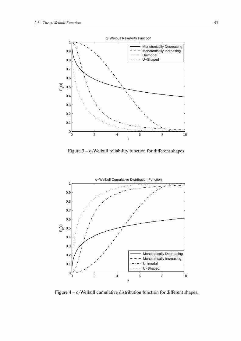
2.3. The q-Weibull Function 53
0 2 4 6 8 100
0.1
0.2
0.3
0.4
0.5
0.6
0.7
0.8
0.9
1
x
Rq(x
)
q−Weibull Reliability Function
Monotonically Decreasing Monotonically Increasing Unimodal U−Shaped
Figure 3 – q-Weibull reliability function for different shapes.
0 2 4 6 8 100
0.1
0.2
0.3
0.4
0.5
0.6
0.7
0.8
0.9
1
x
Fq(x
)
q−Weibull Cumulative Distribution Function
Monotonically Decreasing Monotonically Increasing Unimodal U−Shaped
Figure 4 – q-Weibull cumulative distribution function for different shapes.

54 Chapter 2. The q-Weibull Distribution
2.3.3 Failure Rate Function
The failure rate function is presented by:
hq(t) =fq(t)Rq(t)
=(2 − q)β
η
(t − γη
)β−1expq
− (t − γη
)βq−1
(2.5)
as viewed before, when q → 1 the failure rate for q-Weibull will be reduced to the originalWeibull according to:
h1(t) =β
η
(t − γη
)β−1
(2.6)
0 1 2 3 4 5 6 7 80
0.2
0.4
0.6
0.8
1
1.2
1.4
1.6
x
h q(x)
q−Weibull Failure Rate Function
Monotonically Decreasing Monotonically Increasing Unimodal U−Shaped
Figure 5 – q-Weibull failure rate function for different shapes.
2.3.4 Mean Life Function
The mean life function for q-Weibull distribution with q > 1 is given by:
T =
1∑i=0
γ1−iηiΓ
(1 +
iβ
)Γ(
2−qq−1 −
iβ
)(q − 1)i/βΓ
(2−qq−1
), 1 < q < 1 +β
β + η(2.7)
and for q < 1 is given by:
T =
1∑i=0
γn−iηiΓ
(1 +
iβ
)Γ(
3−2q1−q
)(1 − q)i/βΓ
(3−2q1−q + i
β
), q < 1 (2.8)

2.4. Mathematical Properties and Main Applications for q-Weibull Distribution 55
these two formulations are necessary due to normalization requirements for q < 1 and q > 1.
2.3.5 Median Life Function
The median life function for q-Weibull distribution is given by:
T = γ + η
log 12−q
0.5
q − 2
1β
(2.9)
for all values of q.
2.3.6 Modal Life Function
Modal life function for q-Weibull distribution is given by:
T = γ + η
(β − 1
β + (β − 1)(1 − q)
) 1β
,∀β > 1 (2.10)
for all values of q but with constraints around β.
2.4 Mathematical Properties and Main Applications for q-Weibull
Distribution
One of the main advantages for use q-Weibull distribution is the ability to represent dif-ferent behaviors of failure rate shapes, i.e., monotonically decreasing, monotonically increasing,constant, unimodal and bathtub curves, by changing only q and β parameters according to Table2. This ability has an important aspect in the study of asset life cycle due to the correlationbetween failure rate shape behavior with maintenance strategies choices as can be seen in section1.6.
Table 2 – q-Weibull failure rate behavior.
q-WeibullParameters 0 < β < 1 β = 1 β > 1
q < 1 U-Shape, Bathtub curve Monoton. increasing Monoton. increasingq = 1 Monoton. decreasing Constant Monoton. increasing1 < q < 2 Monoton. decreasing Monoton. decreasing Unimodal
The q-Weibull distribution unifies monotonic and non-monotonic hazard rate functionsby using one general formula. Using a single set of three parameters, q-Weibull can represent thewhole bathtub curve (Figure 6) without piecewise description, which is necessary when using

56 Chapter 2. The q-Weibull Distribution
original Weibull distribution. The flexibility of q-Weibull is important to accurately performreliability analyses when failure data are characterized by non-monotonic hazard rates.
0 10 20 30 40 50 60 70 80 900
0.5
1
1.5
2
2.5
x
h q(x)
q−Weibull Bathtub Curve
q = 0.95 q = 0.9 q = 0.5 q = −1
Figure 6 – q-Weibull bathtub curve for different q parameters.
Examples presented by (ASSIS; BORGES; MELO, 2013) for oil pumps and pumpingrods which presents failure rates with a bathtub shape and another example for production tubingswhich exhibits failure rate as an unimodal function, shows that the performance of q-Weibullwas superior to usual Weibull for all examples when evaluated using goodness of fit and meansquared error (MSE) criteria.
The q-Weibull pdf has not all its moments defined for q > 1, besides all moments arewell defined for q < 1. When parameter q < 1, the maximum allowed time (lifetime deadline)presents divergence when using (2.5) due to the fact that Hq<1 → ∞ at t → tmax < ∞, where H(t)represents the cumulative failure rate function (total number of expected failures at t). Weibulldistribution is unlimited at t, thus Hq=1 → ∞ at t → ∞, q-Weibull is limited at tmax which isdefined by:
tmax = γ + η (1 − q)−1β ,∀q < 1 (2.11)
The method usually applied to estimate the q-Weibull parameters, due to the fact thatthis function has four parameters, is the MLE method. The algorithms commonly used to findefficiently the maximum value for (1.52) are the Nelder-Mead simplex (ARORA, 2012, p. 694–696), ellipsoidal algorithm (SILVA, 2015b) and some class of nature-based heuristic methodslike artificial bee colony, particle swarm optimization and others (XUA et al., 2017).

57
3 Parametric Recurrent Data Analysis
3.1 Introduction
The parametric recurrent event data analysis (RDA) is a field from reliability engineeringconcerned in the study of failure behavior of a specific system and the effects of repairs onthe age of that system. In RDA the events must be statistically dependent and not identicallydistributed such as repairable system data (RELIASOFT RGA, 2009, p. 11). This assumption isthe inverse from LDA which needs events to be IID. Two types of RDA approaches are providedto analyze event data: non-parametric and parametric RDA analysis. This work concerns on thelatter one.
Parametric RDA can be analyzed using perfect renewal process (PRP) when repairdata are corresponding to perfect repairs, i.e., AGAN. For minimal repairs, i.e., as bad as oldrepair (ABAO), RDA uses non-homogeneous Poisson process (NHPP) (GUO et al., 2007). Theintermediate and most complicated scenario when a general repair is better than old, but worsethan new (BOWN), i.e., 0 < R f < 1, RDA treated these events data using general renewal process(GRP) model (KIJIMA; SUMITA, 1986).
3.2 The GRP Model
Failure and repair events can be treated as recurrent data and the rate which these eventsoccur may keep constant, decrease and increase. Past and current repairs may affect future failuresand GRP is useful in modeling the failure behavior of a specific system partially rejuvenatedafter repair, i.e., 0 < R f < 1.
The GRP model uses the concept of virtual age v, i.e., the age of a system right after arepair. An example of equipment aging affected by virtual age can be found at (CASSADY et al.,2005). Figure 7 presents a system with successive failure times t and the corresponding time x
between these failures so that the i-th time failure is the sum of the past xi times according to:
ti =
i∑j=1
x j (3.1)
3.2.1 GRP Model Type I
The GRP model type I assumes that after each event (failure), the repair actions takento improve the system performance will not remove the cumulative damage from previousfailures, i.e., when a i-th failure happens the i-th repair only reduce the additional age xi to q f xi,

58 Chapter 3. Parametric Recurrent Data Analysis
0
X1
t1
X2
t2
X3
t3 tn−2
Xn−1
tn−1
Xn
tn
Figure 7 – System failure times. SOURCE: (RELIASOFT BLOCKSIM, 2007, p. 255)
where parameter q f represents the action effectiveness factor with domain constraints equals to0 ≤ q f ≤ 1. Equation:
vi = vi−1 + q f xi = q f ti (3.2)
presents the virtual age function vi for GRP model type I (METTAS; ZHAO, 2005).
3.2.2 GRP Model Type II
For GRP model type II, the virtual age is given by:
vi = q f (vi−1 + xi) = qif x1 + qi−1
f x2 + . . . + xi (3.3)
In this model type the i-th repair will remove all cumulative damage from both current andprevious failures by reducing the virtual age to q f (vi−1 + xi) (METTAS; ZHAO, 2005).
3.2.3 The Power Law Function
The rate of recurrence for GRP model according to (GUO; ZHAO; METTAS, 2006) isgiven by the power law function:
λ(t) = λβtβ−1 (3.4)
where:λ(t): failure intensity function;λ: recurrence rate;β: shape parameter;t: time.
The characteristic life η can be calculated by:
η =
(1λ
)1/β
(3.5)

3.3. Imperfect Repairs 59
To estimate the power law function parameters λ, β and q f , the conditional pdf derivedfrom (3.4) and given by:
f (ti|ti−1) = λβ (xi + vi−1)β−1 e−λ[(xi+vi−1)β−vβi−1
](3.6)
must be applied to the log likelihood function according to:
Λ = ln(L) = n(ln λ + ln β) − λ[(T − tn + vn)β − vβn
]- λ
n∑i=1
[(xi + vi−1)β − vβi−1
]+ (β − 1)
n∑i=1
ln (xi + vi−1)(3.7)
The constant n is the total number of events during the entire observation period. Time T is thestop observation time of the system, if T stops right after the last event (failure) then T = tn,otherwise T > tn and the stop observation time has the same meaning of a suspension time (GUOet al., 2010).
3.3 Imperfect Repairs
3.3.1 Restoration Factors
The imperfect repairs occur in maintenance tasks when a repair or replacement of suchequipment or component is done with used ones or with new ones but with imperfect repair dueto poor quality of tools, procedures or lack of training for maintenance crews. The best way tomodel an imperfect repair is to give a virtual age to the equipment or component analyzed. Thevirtual age will be affect by the action effectiveness factor q f , described by the GRP model, aftereach repair or maintenance action. Usually R f is given by:
R f = 1 − q f (3.8)
and is used to modeling the restoration factor instead of q f . The following examples extractedfrom (RELIASOFT BLOCKSIM, 2007, p. 253) better describe the concept around restorationfactors:
• restoration factor of 1 (100%) implies that the component is AGAN after repair, i.e., thevirtual age (start age) is set to zero right after a maintenance action. Examples for this caseare the discard tasks like cartridge filter and lamp substitutions;
• restoration factor of 0 implies that the component is ABAO after repair, i.e., the virtual age(start age) is the same as it was prior to repair. The age will be not affected by maintenanceactions. Examples for this case are the restoration tasks with extremely poor qualitymaintenance or discard tasks with used equipments or components with the same age thatthe previous one;

60 Chapter 3. Parametric Recurrent Data Analysis
• restoration factor of 0.30 (30%) implies that the component is BOWN after repair andthe virtual age of the equipment or component is equal to 0.70 (70%) of component’s ageat failure time. Examples are the imperfect maintenance due to restoration tasks such aslubrications, cleaning and screw tightenings.
A detailed effect of imperfect repair in the equipment hazard rate function can be foundat (CHEN et al., 2016) and (LU et al., 2012). Another important aspect over restoration factors isthe fact that if a failure distribution is modeled by exponential functions, the restoration factors q f
or R f do not make any effect in the final age of equipment or component. The same analogy canbe done with effect of preventive maintenance with equipment failures modeled by exponentialfunctions.
3.3.1.1 Restoration Factor Type I
Imperfect repairs modeled by restoration factor type I uses GRP model type I (3.2) toremove only the damage caused by current failure (KIJIMA, 1989). The Algorithm 1 based onexample extracted from (RELIASOFT BLOCKSIM, 2007, p. 256) was proposed to implementthis restoration model. Figure 8 presents the simulation time results up to the second failureusing Algorithm 1.
Algorithm 1 Example for R f type I algorithmInput: β, η, R ftype−I
Output: ti
1: f (t)← W(β, η) . Choose a specific distribution, e.g., Weibull with β = 1.5 and η = 1000h2: q f ← 1 − R f . Set action effectiveness factor equal to 70% (R f =30%)3: v0 ← 0 . Set initial virtual age to zero4: p1 ← U1[0, 1] . Generate an uniform random number, e.g., U1 = 0.70225: x1 ← F−1(p1) . Calculate the first time between failure using unreliable life with probability
calculated from step 4, e.g., x1 = 500h6: t1 ← x1 . Calculate the first time failure, e.g., t1 = 500h7: v1 ← v0 + q f x1 . Calculate the virtual age right after the first failure, e.g., v1 = 350h8: for i = 2→ n do . Implement a loop from second to n-th failure9: pi ← Ui[0, 1] . Generate an uniform random number, e.g., U2 = 0.8825
10: xi ← F−1[piR(vi−1)] − vi−1 . Calculate the i-th time between failure using conditionalreliability function R(t + T ) = R(t,T )R(T ). Example: x2 = 129.53
11: ti ← ti−1 + xi . Calculate the i-th time failure, e.g., t2 = 629.5312: vi ← vi−1 + q f xi . Calculate the i-th virtual age right after the i-th failure, e.g.,
v2 = 440.6713: end for
3.3.1.2 Restoration Factor Type II
The Algorithm 2, based on example extracted from (RELIASOFT BLOCKSIM, 2007,p. 257), was proposed to implement imperfect repairs modeled by restoration factor type II (3.3).

3.3. Imperfect Repairs 61
time (h)ta,b0 = 0
va,b0 = 0
R f
RafI
= 1.00
RbfI
= 0.30
xa,b1 = 500
ta,b1 = 500va
1 = 0vb
1 = 350
xa2 = 250
ta2 = 750va
2 = 0
xb2 = 129.53
tb2 = 629.53
vb2 = 440.67
Figure 8 – Failure times for R f type I example.
This restoration model remove all cumulative damage from both current and previous failures(KIJIMA, 1989). Simulation time results up to the second failure using GRP model type II ispresented by Figure 9. An important fact about the two simulations examples given by Figures8 and 9 refers to the time which occurs the second failure. With the start age equal to zeros inboth examples, even with different R f types, the time to occurs the second failure is the same butthe virtual age after second failure is different. These effects will influence the third and othersfailure times.
Algorithm 2 Example for R f type II algorithmInput: β, η, R ftype−II
Output: ti
1: f (t)← W(β, η) . Choose a specific distribution, e.g., Weibull with β = 1.5 and η = 1000h2: q f ← 1 − R f . Set action effectiveness factor equal to 70% (R f =30%)3: v0 ← 0 . Set initial virtual age to zero4: p1 ← U1[0, 1] . Generate an uniform random number, e.g., U1 = 0.70225: x1 ← F−1(p1) . Calculate the first time between failure using unreliable life with probability
calculated from step 4, e.g., x1 = 500h6: t1 ← x1 . Calculate the first time failure, e.g., t1 = 500h7: v1 ← q f (v0 + q f x1) . Calculate the virtual age right after the first failure, e.g., v1 = 350h8: for i = 2→ n do . Implement a loop from second to n-th failure9: pi ← Ui[0, 1] . Generate an uniform random number, e.g., U2 = 0.8825
10: xi ← F−1[piR(vi−1)] − vi−1 . Calculate the i-th time between failure using conditionalreliability function R(t + T ) = R(t,T )R(T ). Example: x2 = 129.53
11: ti ← ti−1 + xi . Calculate the i-th time failure, e.g., t2 = 629.5312: vi ← q f (vi−1 + xi) . Calculate the i-th virtual age right after the i-th failure, e.g.,
v2 = 335.6713: end for

62 Chapter 3. Parametric Recurrent Data Analysis
time (h)ta,b0 = 0
va,b0 = 0
R f
RafII
= 1.00
RbfII
= 0.30
xa,b1 = 500
ta,b1 = 500va
1 = 0vb
1 = 350
xa2 = 250
ta2 = 750va
2 = 0
xb2 = 129.53
tb2 = 629.53
vb2 = 335.67
Figure 9 – Failure times for R f type II example.
3.3.2 Restoration Factor Calculus
The parameters that needs to be estimated in GRP model are λ, β, η and q f (R f ). In thiswork, a MATLAB code was developed to estimate these parameters using the log likelihoodfunction (3.7). This MATLAB code uses constrained optimization to find the optimum parametersthat maximizes (3.7) (MATHWORKS, 2003, p. 2/9). To test the algorithm, an example extractedfrom (RELIASOFT WEIBULL, 2005, p. 418) using ReliaSoft Weibull++ software was used.The set of data failures are respected from an air-conditioning unit of an aircraft (Table 3).Table 4 compares the results for estimated parameters obtained from Weibull++ software withparameters obtained from MATLAB code implemented, the error was bellow 0.1%. To comparethe results, it was used the mean absolute percentage error (MAPE):
EM =1n
n∑t=1
|yt − y′
t |
|yt|100 (3.9)
Table 3 – Air-conditioning failure data. SOURCE: (RELIASOFT WEIBULL, 2005, p. 418)
50 290 544 945 1013 148994 329 732 950 1152 1512
196 332 811 955 1362 1525268 347 899 991 1459 1539
Table 4 – Estimated parameters comparison.
Parameters Weibull++ MATLAB MAPE
λ 4.94E-3 4.9419E-3 0.0385%β 1.19760 1.19760 0.0000%η 84.2841 84.2690 0.0179%q 0.13440 0.13451 0.0818%

63
4 Optimum Maintenance Intervals
4.1 Preventive Maintenance Interval Models
Calculation of optimum PM intervals is one of the biggest challenges in a maintenanceprogram. The use of incorrect intervals can lead the equipment to operate in non-profit scenarioeven though maintenance strategy was adjusted correctly. Many qualitative and quantitativemethods exists in literature to determine the optimum intervals, since the most easy methodlike Age Exploration – applied only when good statistical data is not available and experienceto guess at task intervals is really the only option – until advanced statistical methods whichuses distributions functions obtained from equipments life data. The following methods used tocalculate optimum PM intervals are briefly described:
4.1.1 Age Exploration
The age exploration (AE) technique is strictly empirical. It works like this illustrativeexample: supposing an initial overhaul interval for a fan motor is 3 years and after the firstoverhaul, inspections reveals no such wearout or aging signs, than the initial interval is increasedautomatically by 10%. Repeat the process, continuing until, on one of the overhauls, incipientsigns of wearout or aging are inspected. At this point, the AE process stops, perhaps back off by10%, and define this as the final task interval (SMITH; HINCHCLIFFE, 2003, p. 126–127).
4.1.2 Optimal Preventive Replacement Interval
Preventive maintenance actions, i.e., actions taken before equipment reaches a failedstate, require two necessary conditions to be implemented: (i) the total cost of the replacementmust be greater after failure than before and; (ii) the hazard rate of the equipment must beincreasing (JARDINE; TSANG, 2013, p. 38). From mathematical theory of optimization, thegeneral formulation of an optimization problem is expressed by:
x∗ = arg minx
f (x) ∈ Rm, x ∈ F
F = {x ∈ Rn | g(x) ≤ 0, h(x) = 0}(4.1)
where f (x) represent the function to be minimized or maximized, g(x) and h(x) the constraintsfunctions of the problem. Both cost-based and downtime-based models used to optimize PMintervals are also expressed by this formulation.

64 Chapter 4. Optimum Maintenance Intervals
where:x∗: vector of optimum variables;f (x): objective function f : Rn 7→ R;R: real set numbers;F: feasible set;g(x): inequality constraint function g : Rn 7→ Rm;h(x): equality constraint function h : Rn 7→ Rp;x: vector of optimization variables.
4.1.2.1 Cost-Based Models
If cost, due to the high cost of replacement after failure, is the appropriate criterion tobe applied as objective function to determine PM interval, then a cost-based model is desired.A model proposed by (BARLOW; HUNTER, 1960) determine the optimum age time for PMaction which minimizes global costs:
t∗c = mint
fc(t) =CpR(t) + Cu(1 − R(t))∫ t
0R(t)dt
(4.2)
where:t∗c: optimum age cost-based PM interval;fc(t): age PM cost function fc : R 7→ R;R(t): reliability function R : R 7→ R;Cp: cost of preventive task;Cu: cost of corrective task;t: time.
An alternative formulation for age cost-based models are also presented by (JARDINE; TSANG,2013, p. 52):
t∗c = mint
fc(t) =CpR(t) + Cu(1 − R(t))
tR(t) +∫ t
0t f (t)dt
(4.3)
where:f (t): probability density function.
cost-based models can also be applied to the study of predictive maintenance intervals optimiza-tions (SILVA; SALDANHA; LISBOA, 2017b).
4.1.2.2 Downtime-Based Models
For cases which the objective is to get maximum throughput or utilization of equipment,the PM interval required may be one which minimizes total downtime per unit time. When PMinterval decrease, the number of CM and availability also decreases due to the higher number of

4.1. Preventive Maintenance Interval Models 65
PM performed. On the other hand if PM interval increase, the number of CM due to failures alsoincreases leading the availability decrease due to CM performed. According to:
t∗d = mint
fd(t) =TpR(t) + Tu(1 − R(t))
(t + Tp)R(t) +[∫ t
0R(t)dt + Tu
](1 − R(t))
(4.4)
where:t∗d: optimum age downtime-based PM interval;fd(t): age PM downtime function fd : R 7→ R;Tp: time to perform preventive task;Tu: time to perform corrective task.
the perfect balance age time interval is obtained to perform preventive and corrective repairtasks that minimizes downtime of the equipment. Also, an age alternative formulation foravailability-based models are presented by (JARDINE, 1973, p. 94–96):
t∗d = mint
fd(t) =TpR(t) + Tu(1 − R(t))
(t + Tp)R(t) +∫ t
0t f (t)dt + Tu(1 − R(t))
(4.5)
For cases which the calendar time must be used, formulation:
t∗d = mint
fd(t) =H(t)Tu + Tp
t + Tp(4.6)
where:t∗d: optimum calendar downtime-based PM interval;fd(t): calendar PM downtime function fd : R 7→ R;H(t): expected number of failures function H : R 7→ R.
presented by (JARDINE, 1973, p. 95) calculate the optimum calendar PM interval.
4.1.2.3 Cost and Downtime Based Models
According to (JARDINE, 1973, p. 92–94), an alternative formula for PM age intervalwhich optimizes both cost and availability is presented by:
t∗cd = mint
fcd(t) =CpR(t) + Cu(1 − R(t))
(t + Tp)R(t) +∫ t
0t f (t)dt + Tu(1 − R(t))
(4.7)
where:t∗cd: optimum calendar cost and downtime based PM interval;fcd(t): calendar PM cost and downtime function fcd : R 7→ R.

66 Chapter 4. Optimum Maintenance Intervals
4.2 A Practical Optimization Model In The MRGF Indicator
4.2.1 Definition
The indicator for mechanism reduction of physical guarantees (MRGF, or the old MRA,guaranteed energy reduction mechanism) aims to encourage the quality of electric energy gener-ation service (LISBOA et al., 2015). This indicator verifies whether a power plant participant ofenergy relocation mechanism (MRE) has fulfilled or not the established availability requirements.These verifications are made by calculating an availability factor ηi, equivalent to the ratiobetween verified indexes ( fi and pi) and the reference indexes ( fi and pi) (LISBOA et al., 2015).This availability factor is given by:
ηi = min{
1,(1 − fi)(1 − pi)(1 − fi)(1 − pi)
}(4.8)
where:ηi: availability factor;fi: forced interruption rate index;fi: reference index for forced interruption rate;pi: planned interruption rate index;pi: reference index for planned interruption rate.
These parameters in (4.8) are calculated within a 60-month time window, includingthe backward calculation month. The reference indexes are provided by the Brazilian electricnational system operator (ONS) and agents, being statistical parameters that cannot be controlledby the agent at first. The forced interruption rate can be controlled indirectly by the agent, e.g.,through preventive maintenance, while the planned interruption rate is naturally over the controlof the agent. These interruptions are typically justified by preventive maintenance at the plants.A value less than 1 for ηi means that the plant has not met the availability requirements, and itsphysical guarantee will be adjusted to reflect this non-compliance (LISBOA et al., 2015). Theformulation of MRGF can be found in the marketing rules of the Brazilian marketing chamberof electric energy (CCEE) (CCEE, 2017; CCEE, 2016).
4.2.2 Applicability
Physical guarantee is what has commercial value in the energy market, not the energyactually generated. Therefore, the physical guarantee of a power plant must be maximizedto avoid loss of revenue. In addition, loss of availability may imply a reduction of physicalguarantee, which is a key factor of electric system operation (LISBOA et al., 2015).
The main objective of a power plant is to maximize the availability of energy generationwith quality. For maximizing the availability, many strategies could be used. One of the mostused is the PM time optimization. As mentioned before, the correct preventive maintenance

4.3. Mathematical Analysis for Optimization Problems 67
interval reduces the number of outages (failures) in equipments, increasing the availability, anddecreasing the failure number and cost. An objective function can be adjusted to optimize theavailability of an electric system according to:
t∗ = arg maxt
A(t) = (1 − fi(t))(1 − pi(t)), t ∈ F :
F = {t ∈ R | T ≤ t ≤ T }(4.9)
where:t∗: optimum PM interval;A(t): availability function A : R 7→ R;fi(t): forced interruption rate function f : R 7→ R;pi(t): planned interruption rate function p : R 7→ R;F: feasible set;R: real set numbers;T : time to perform PM repair;T : time which availability turn to zero;t: time.
This expression is exactly the availability factor ηi in (4.8) without the references indexes andthe upper bound at 1.
4.3 Mathematical Analysis for Optimization Problems
The cost and downtime based models discussed previously must be analyzed in respect ofconvexity and unimodality to assure that the optimizations algorithms used, especially algorithmsbased in gradients evaluations like ellipsoidal, Broyden-Fletcher-Goldfarb-Shanno (BFGS) oreven Nelder-Mead algorithm, will reach the global optimum solution.
According to (BOYD; VANDENBERGHE, 2009, p. 67), a function f : Rn 7→ R isconvex if dom f is a convex set and if for all x, y ∈ dom f , and θ with 0 ≤ θ ≤ 1, thus:
f (θx + (1 − θ)y) ≤ θ f (x) + (1 − θ) f (y) (4.10)
Geometrically, this inequality means that the line segment between (x, f (x)) and (y, f (y)), whichis the chord from x to y, lies above the graph of function f . The mathematical condition toestablish an unimodal function is that the first derivative is null at only one point in the subinterval[t1, t2] of the function domain. The unimodality can also be guaranteed if:
f ′′(T ) ≤f ′(T )2
f (T ),∀T ∈ [t1, t2] (4.11)
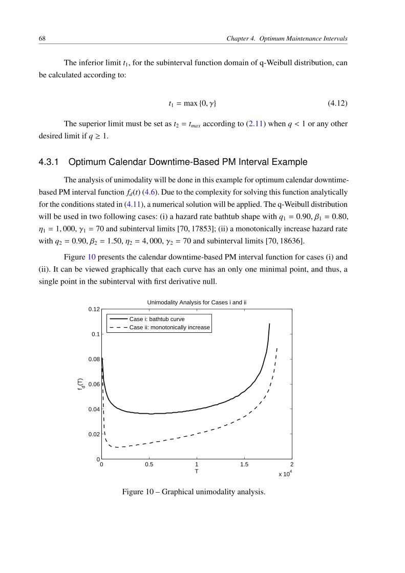
68 Chapter 4. Optimum Maintenance Intervals
The inferior limit t1, for the subinterval function domain of q-Weibull distribution, canbe calculated according to:
t1 = max {0, γ} (4.12)
The superior limit must be set as t2 = tmax according to (2.11) when q < 1 or any otherdesired limit if q ≥ 1.
4.3.1 Optimum Calendar Downtime-Based PM Interval Example
The analysis of unimodality will be done in this example for optimum calendar downtime-based PM interval function fd(t) (4.6). Due to the complexity for solving this function analyticallyfor the conditions stated in (4.11), a numerical solution will be applied. The q-Weibull distributionwill be used in two following cases: (i) a hazard rate bathtub shape with q1 = 0.90, β1 = 0.80,η1 = 1, 000, γ1 = 70 and subinterval limits [70, 17853]; (ii) a monotonically increase hazard ratewith q2 = 0.90, β2 = 1.50, η2 = 4, 000, γ2 = 70 and subinterval limits [70, 18636].
Figure 10 presents the calendar downtime-based PM interval function for cases (i) and(ii). It can be viewed graphically that each curve has an only one minimal point, and thus, asingle point in the subinterval with first derivative null.
0 0.5 1 1.5 2
x 104
0
0.02
0.04
0.06
0.08
0.1
0.12
T
f d(T)
Unimodality Analysis for Cases i and ii
Case i: bathtub curveCase ii: monotonically increase
Figure 10 – Graphical unimodality analysis.

69
5 Maintenance Strategies Simulation
5.1 Monte Carlo Reliability Simulation
5.1.1 Introduction
Simulations are used to predict the behavior of processes or equipments whose operationare difficult or impossible to represent with analytical models. They also may be used if themathematical relationships are known but would require more time than the simulation process.Reliability simulation are primarily discrete model with a governing sequence of discrete events,such as failures, corrective repairs, preventive maintenance actions and equipment or componentstand-by switchings. The role of reliability simulation is the creation of an algorithm whichtransforms a set of initial data into a sequence of discrete events. These events may havestatistical characteristics that must be computed at each completed simulation run (USHAKOV;HARRISON, 1994, p. 456).
Monte Carlo simulation was first proposed in the 40’s by mathematicians John vonNeumann and Stanislaw Ulam from Manhattan project in Los Alamos - USA, for evaluatingcomplicated mathematical integrals that arise in the theory of nuclear chain reactions. Thissimulation method allow the solution to mathematical and technical problems by means ofsystem probabilistic models and simulation of random variables. Playing an important role insystem reliability, availability and optimal maintenance of large-scale complex networks, MonteCarlo simulation is now recognized as relatively easy and fast analysis method for determiningstandard confidence bounds of complex reliability system (WANG; PHAM, 2006, p. 275–276).
5.1.2 Distributed Pseudo Random Number Generator
The basis of Monte Carlo simulation is the random variables inputs generated by a pseudorandom number generator (RNG) to simulate the process of sampling from a population. Thesepseudo random variables are generated following an arbitrary statistical distribution accordingto specific needs of the simulation problem. The ability to generate pseudo random numbers isthe key for a successful Monte Carlo simulation. The uniform distribution holds a special placein the Monte Carlo simulation due to the fact that any RNG can use the uniformly distributedrandom variable for the RNG process (O’CONNOR; KLEYNER, 2012, p. 108–109).
The continuous uniform distribution, a.k.a., rectangular distribution, has constant proba-

70 Chapter 5. Maintenance Strategies Simulation
bility on the interval [a, b] (Figure 11) and pdf given by:
f (x) =
1(b−a) , a ≤ x ≤ b,
0, otherwise.(5.1)
In cases which a specific value must have higher probability of occurrence, the triangulardistribution can be used. Such distribution is often used in engineering approximations where arandom variable is defined by the minimum, most likely and maximum values, also referred asthree-point estimator (O’CONNOR; KLEYNER, 2012, p. 109).
x
f (x)
a b
1(b−a)
Figure 11 – Uniform distribution. SOURCE: (O’CONNOR; KLEYNER, 2012, p. 110)
One of the most applied methods for generate a custom distribution of pseudo randomnumbers is the inverse-transform method. This method is quite simple and easy to implement.The process begins with the generation of a probability value Ui obtained from an uniformdistribution U(0, 1), then using a chosen distribution, the inverse cdf is calculate for Ui giventhe pseudo random value for X that represents the random number generated by the chosendistribution. Figure 12 and Algorithm 3 illustrated the whole process (KROESE; TAIMRE;BOTEV, 2011, p. 45).
Algorithm 3 Inverse-transform algorithmInput: D(θ1, θ2, ..., θk), mOutput: X
1: for i = 1→ m do . Implement a loop from 1 to max number of simulations m2: Ui ← U(0, 1) . Generate an uniform probability value3: Xi ← F−1(Ui; θ1, θ2, ..., θk) . Calculate the inverse cdf for Ui
4: end for
5.1.3 Number of Simulation Runs
The total number of runs necessary in a Monte Carlo simulation depends on the accuracyrequired, the complexity of the deterministic model, variance of the input and the sought accuracyof the output. High variance of the input and high complexity of the model increases the variance

5.1. Monte Carlo Reliability Simulation 71
x
F(x)
1
U
0X
Figure 12 – Inverse-transform method.
of the output and thus more simulation runs are required to achieve the stability of the output(O’CONNOR; KLEYNER, 2012, p. 112).
An estimation for the numbers of runs to reach a certain level of confidence in statisticsof the simulated output can be implemented by using the central limit theorem and the confidencebounds estimate for the normal distribution. The appropriate sample size is found by calculate m:
m =
(Zα/2σEr(µ)
)2
(5.2)
where:m: number of Monte Carlo runs;Zα/2: standard normal statistic;α = 1 −C: significance level, where C is the confidence level;σ: standard deviation of the output;Er(µ) = |x − µ|: standard error of the mean.
this formulation calculates the sample size with specified error on the mean with variance known(MONTGOMERY; RUNGER, 2011, p. 256). This formulation has limited applications becausethe value of σ is not known and can only be assumed a priori or estimated after the first simulation(CHAN, 2013, p. 29-34).
5.1.4 Basic Monte Carlo Simulation Algorithm
A Monte Carlo algorithm could vary based on the scope of the problem. A diagram toillustrate this process can viewed at (GOTI, 2010, p. 110). The core of the algorithm can beimplemented using basic steps according to (O’CONNOR; KLEYNER, 2012, p. 112):
• step 1: define the problem and the overall objectives of the study. Evaluate the availabledata and outcome expectations;

72 Chapter 5. Maintenance Strategies Simulation
• step 2: define the system and create a parametric model, y = f (x1, x2, ..., xq);
• step 3: design the simulation. Quantities of interest need to be collected, such as theprobability distributions for each of the inputs. Define how many simulation runs shouldbe used. The number of runs m is affected by the complexity of the model and the soughtaccuracy of results;
• step 4: generate a set of random inputs, xi,1, xi,2, ..., xi,q;
• step 5: run the deterministic system model with the set of random inputs. Evaluate themodel and store the results as yi;
• step 6: repeat steps 4 and 5 until i = m;
• step 7: analyze the overall results like confidence intervals, histograms, best fit distributionor any other statistical measure.
5.2 Maintenance Scenarios Simulation
5.2.1 Introduction
The maintenance scenarios simulated in the following subsections are basically teststo validate the Monte Carlo algorithm developed in MATLAB, called maintenance strategiessimulator (MSS), to test the analytical functions used to optimize the asset availability modelsdeveloped in this work. To compare such simulation results, it was used a worldwide benchmarkreliability simulation software called ReliaSoft BlockSim 7, version 7.0.14. To quantify errorsbetween MATLAB MSS and BlockSim 7, the MAPE error was used (3.9).
The simulation parameters used in BlockSim 7 and MATLAB MSS are describedaccording to Table 5. The q-Weibull distribution with parameter q = 1 was used to simulatedWeibull 2-parameters, due to the fact that q-Weibull had not yet been implemented by BlockSim7 software.
Table 5 – Simulation parameters.
Parameters Values
Failure Distribution q-Weibull (q = 1; β = 2.5; η = 1200h; γ = 0)CM TTR Distribution constant = 50hPM TTR Distribution constant = 15hPM Calendar Interval constant = 800hSimulation Time (h) 5000hNumber of Simulations 5000Increments Calculations 10

5.2. Maintenance Scenarios Simulation 73
5.2.2 Corrective Maintenance Simulation
5.2.2.1 Non-Corrective Maintenance
The first simulated maintenance scenario used to test MATLAB MSS, was the case fornon-corrective maintenance. It’s expected that the availability value in this scenario was very lowdue to the fact that no maintenance strategies are made to improve availability. The simulationprocess for this scenario is quite easy due to the fact that no maintenance strategies are made,the simulation generates just one TTF, i.e., TT F1, for each simulation time tsim. Operational(non-failure) and failure states are represented respectively by letters O and F according toFigure 13.
An important parameter obtained in this simulation is the mean time to first failure(MTTFF), this parameter is the arithmetic mean for all time to first failure (TTFF) valuesgenerated in the entire number of simulations, this parameter also helps to evaluate the quality ofRNG when no maintenance strategies are applied. Figure 14 presents the evolution for availabilityparameter during the total number of simulations.
x
Op. S tate
O
S
F0 tsim
TT FF = TT F1
Figure 13 – Simulation example for non-corrective maintenance.
Table 6 presents the simulation results for BlockSim 7 and MATLAB MSS. It can beseen that the MAPE error was very low for all parameters compared.
5.2.2.2 Corrective Maintenance With Perfect Repair
The next simulated scenario used the most basic maintenance strategy, the correctivemaintenance. Naturally, the availability must be greater than with no maintenance scenario. Thecomplexity in this simulation process increases due to the fact that many conditions must be met.An example about this, is the number of failures and repairs that are done until the simulationtime is reached. In case of failures or repairs, the TTF or TTR generated should be truncated toavoid failures or repairs occurring after the final simulation time. Figure 15 presents the mainsimulation process idea applied for this scenario.

74 Chapter 5. Maintenance Strategies Simulation
0 1000 2000 3000 4000 500020
20.5
21
21.5
22
22.5
23
23.5
24
24.5
25Maintenance Strategies Simulation
Upt
ime
%
Simulation Number
Non−corrective maintenance
Figure 14 – Simulation for non-corrective maintenance.
Table 6 – Simulation results for non-corrective maintenance.
Simulation Parameters BlockSim 7 MATLAB MSS MAPE
Uptime 0.2132 0.2133 0.0296%Mean Uptime (h) 1066.1614 1066.3173 0.0146%Mean CM Time (h) NE NE NEMean PM Time (h) NE NE NEMTTFF (h) 1066.1614 1066.3173 0.0146%# Total Failures 1 1 0.0000%# CM NE NE NE# PM NE NE NE
The simulation results for CM with perfect repair using BlockSim 7 and MATLAB MSSare displayed by Table 7. The MAPE error evaluated for each parameters compared are still low.
5.2.2.3 Corrective Maintenance With Non-Perfect Repair
Simulation using corrective maintenance with non-perfect repair is very similar whenusing perfect repair simulation. The main difference lies in the failure times that are recalculatedusing restoration factors and GRP models approached in details in sections 3.2 and 3.3. In Figure16, the failure time F1.0
2 represents the second simulation failure with perfect repair, i.e., R f = 1.0,this failure time is the same as presented by Figure 15. With non-perfect repair, the second andforward failures are different and must be recalculated according to R f values and restorationfactor types. This behavior occurs due to the fact that after each maintenance, the age of the

5.2. Maintenance Scenarios Simulation 75
x
Op. S tate
O
S
F0 tsim
TT FF = TT F1
TTR1
TT F2
TTR2
TT F3
Figure 15 – Simulation example for corrective maintenance with perfect repair.
Table 7 – Simulation results for corrective maintenance with perfect repair.
Simulation Parameters BlockSim 7 MATLAB MSS MAPE
Uptime 0.9590 0.9592 0.0224%Mean Uptime (h) 4794.7956 4796.0753 0.0267%Mean CM Time (h) 205.2044 203.9247 0.6236%Mean PM Time (h) NE NE NEMTTFF (h) 1060.0269 1069.3893 0.8832%# Total Failures 4.1282 4.1012 0.6540%# CM 4.1282 4.1012 0.6540%# PM NE NE NE
equipment are reduced by a quantity proportional to the operating time (PHAM, 2003, p. 330).Failure F0.6
2 in Figure 16 illustrates the second failure with TTF adjusted according to non-perfectrepair.
x
Op. S tate
O
S
F0 tsim
TT FF = TT F1
TTR1
TT F2
F0.62 F1.0
2
TTR2
TT F3
Figure 16 – Simulation example for corrective maintenance with non-perfect repair.

76 Chapter 5. Maintenance Strategies Simulation
Tables 8 and 9 presents the simulation results for BlockSim 7 and MATLAB MSS usingrestoration factor of R f = 0.6 with GRP models type I and II respectively. The MAPE errorevaluated remains low for all parameters compared.
Table 8 – Simulation results for corrective maintenance with non-perfect repair (R f =0.6 type I).
Simulation Parameters BlockSim 7 MATLAB MSS MAPE
Uptime 0.9046 0.9048 0.0192%Mean Uptime (h) 4523.1535 4523.8688 0.0158%Mean CM Time (h) 476.8465 476.1312 0.1500%Mean PM Time (h) NE NE NEMTTFF (h) 1062.8797 1064.4665 0.1493%# Total Failures 9.6280 9.6074 0.2140%# CM 9.6280 9.6074 0.2140%# PM NE NE NE
Table 9 – Corrective maintenance with non-perfect repair (R f =0.6 type II) simulation results.
Simulation Parameters BlockSim 7 MATLAB MSS MAPE
Uptime 0.9412 0.9415 0.0260%Mean Uptime (h) 4706.1128 4707.2272 0.0237%Mean CM Time (h) 293.8872 292.7728 0.3792%Mean PM Time (h) NE NE NEMTTFF (h) 1061.6259 1065.8491 0.3978%# Total Failures 5.9110 5.8914 0.3316%# CM 5.9110 5.8914 0.3316%# PM NE NE NE
Figure 17 presents the evolution for availability parameter during the total number ofsimulations for three different maintenance strategies, i.e., perfect CM and non-perfect type I andII CM. It can be seen graphically that perfect repair brings best availability followed respectivelyby type II and I GRP models. Other examples of gains in maintenance strategy under imperfectmaintenance can be found at (LIU; HUANG, 2010).
5.2.3 Preventive and Corrective Maintenance Simulation
The last scenario simulated was applied for preventive and corrective maintenancestrategy. This simulation scenario is, by far, the most complex scenario up to now. The mainreason for the complexity lies in managing lots of variables and conditions related to failures,repairs and preventive intervals.
Figure 18 shows a simulation representation for PM task occurring at PMi interval. Forcases when the TTF occurs before PMi, a failure will occur and corrective repair must be done,this is the situation for CM scenario. Otherwise, if TTF occurs after PMi, a PM task must be done

5.2. Maintenance Scenarios Simulation 77
0 1000 2000 3000 4000 500090
91
92
93
94
95
96
97Maintenance Strategies Simulation
Upt
ime
%
Simulation Number
CM with perfect repairCM with RF = 0.6 type IICM with RF = 0.6 type I
Figure 17 – Simulation for corrective maintenance.
by PM repair time TTR2, reducing the number of failures and thus increasing the availability ofthe equipment. Figure 18 presents this situation when a PM task is realized at PMi time and avirtual failure occurring at F1.0
2 time.
The time to suspension (TTS) represented in Figure 18 is the time before PM, PdMor inspection tasks and do not represent a failure. In LDA, this suspension time is modeled asa quasi-failure and have influence in the way that distribution parameters are estimated. Thequasi-failure (suspension) level are represented by suspended-state in Figure 18.
x
Op. S tate
O
S
F0 tsim
TT FF = TT F1
TTR1
TTS 1
PMi F1.02
TTR2
TT F3
Figure 18 – Simulation example for preventive and corrective maintenance with perfect repair.
The results for PM and CM with perfect repair using BlockSim 7 and MATLAB MSS

78 Chapter 5. Maintenance Strategies Simulation
are presented by Table 10. The MAPE error evaluated remains low except for mean PM time,MTTFF and number of PM realized. This issue is explained by the fact that BlockSim 7 softwareuses age time to perform PM, while MATLAB MSS uses calendar time. Unfortunately, BlockSim7 version 7.0.14 does not allow the calendar time option to perform PM tasks.
Table 10 – Simulation results for preventive and corrective maintenance with perfect repair.
Simulation Parameters BlockSim 7 MATLAB MSS MAPE
Uptime 0.9677 0.9617 0.6213%Mean Uptime (h) 4838.3366 4808.4422 0.6179%Mean CM Time (h) 97.0832 98.0508 0.9967%Mean PM Time (h) 64.5803 93.5070 NEMTTFF (h) 2433.7387 612.8385 NE# Total Failures 1.9492 1.9674 0.9337%# CM 1.9492 1.9674 0.9337%# PM 4.3094 6.2338 NE
Figure 19 shows the evolution for availability parameter through the entire simulationtime for both CM and PM with CM strategies simulated. It can be seen that even with non-optimized preventive time, the mean availability for PM with CM are greater than with only CM.Otherwise this assumption could be wrong if the PM interval are short and PM repair time areclose to CM repair.
0 1000 2000 3000 4000 500095
95.2
95.4
95.6
95.8
96
96.2
96.4
96.6
96.8
97Maintenance Strategies Simulation
Upt
ime
%
Simulation Number
CM and PM with perfect repairCM with perfect repair
Figure 19 – Simulation for preventive and corrective maintenance.

79
6 Experimental Results
6.1 The Onshore Wind Turbine Case
The technology of wind turbines for generating electricity dates back to the end ofnineteenth century. Modern large wind turbines developments date back to work in Europeand the United States, later stimulated by oil price rises after the 1973 Yom Kippur War. Windturbines failures are normally resulting of an unacceptable operational condition, such as an over-temperature, over-speed or pitch problem. Exceptions may occur due to gearbox degradation,generator or blade failures (TAVNER, 2012, p. 1). The basic structure of a modern three-blade,upwind horizontal axis wind turbine is exemplified by Figure 20, with typical mechanical andelectrical variable speed circuit presented by Figure 21.
Figure 20 – 2MW wind turbine layout and terminology. SOURCE: (CHUNG et al., 2016, p. 166)
Figure 21 – Typical wind turbine conversion architectures. SOURCE: (CHUNG et al., 2016,p. 167)
The stochastic nature of mechanical or electrical equipment failures, significantly influ-ence the availability of a wind turbine. The importance of knowing this availability has motivatedseveral studies of reliability, since consumers, mainly commercial and industrial sectors, are

80 Chapter 6. Experimental Results
increasingly sensitive to profit losses associated with unavailability of electrical system (SILVAet al., 2017).
Power system reliability indexes are also an good alternative to model failures and repairsto perform reliability and availability analysis of a wind turbine. The IEEE standards (IEEE,2012) and (IEEE, 2007) give the main concepts to develop RAM analysis in any functionalreliability power system zones, i.e., generation, transmission and distribution, (BROWN, 2002,p. 1–4). Methods like fault tree analysis (FTA) and reliability block diagrams (RBD) are alsouseful to model the entire wind turbine and to perform RAM analysis.
Offshore wind turbine reliability and maintenance costs are of key interest to wind farmoperators, since a high degree of uncertainty area associated with cost and reliability indexes. Tocontrol and achieve risk reduction, models need to be developed in order to predict what is aneglected and important part of wind farm life cycle cost. Maintenance databases are useful toextract metrics which can be used for populating a reliability, risk and maintenance cost model(KARKI; BILLINTON; VERMA, 2014, p. 169–171). Table 11 presents fault occurrence rate peryear for main wind turbine components.
Table 11 – Fault occurrence rate by asset group. SOURCE: (KARKI; BILLINTON; VERMA,2014, p. 172)
Asset name Failure rate/year
Controller 2.362Nacelle 1.391Tower 1.221Transmission 1.091Gearbox 0.841Hub 0.490Parking brake 0.380Hydraulics 0.360Yaw 0.270Generator 0.230Pitch 0.220Measurements sensors 0.210Blade system 0.060Switchgear 0.060Over speed protection system 0.040HV system 0.040
6.1.1 Wind Turbine Gearbox Database
According to chapter 1, an accurate method to predict failure events is the use ofprobability distributions for the time to failure data vector. The failure vectors in Table 12,presents the TTF and accumulated TTF for the wind turbine gearbox from a wind farm located

6.2. Wind Turbine Gearbox Reliability Analysis 81
in Brazil. This power plant has 72 wind turbines installed each one with 2 MW and have been inoperation for 3 years.
The total number of failures where 5, with just one failure for each wind turbine. Thus,five wind turbines failed and 67 still operating without failures. The negative values in both datavectors are representations for right censoring times, i.e., suspensions, and represents the timebetween the beginning of wind turbine operation and the time when data were collected.
Table 12 – Gearbox TTF data
Data Type TT F1 TT F2 TT F3 TT F4 TT F5 TTS 1
TTF 5552 5208 2376 168 7536 -1792TTF Accum. 5552 10760 13136 13304 20840 -22632
6.2 Wind Turbine Gearbox Reliability Analysis
6.2.1 Gearbox Life Data Analysis
The LDA process starts chosen a distribution to estimate parameters for failure data fromTable 12. In this work, the q-Weibull was chosen due to the life cycle characteristics explained insection 2.4. To perform LDA in gearbox, a test must be made to MATLAB MSS algorithm de-veloped to estimated the q-Weibull parameters. This algorithm implemented the MLE estimationparameter method according to subsection 1.11.4. Table 13 was used to test the algorithm, thefailure data values are obtained from the widget example in (RELIASOFT WEIBULL, 2005,p. 177). To test the algorithm, parameter q was set to one, thus the algorithm could be comparedwith Weibull++ 7 software that used bi and tri-parametric Weibull distribution.
Table 13 – Widget failure data. SOURCE: (RELIASOFT WEIBULL, 2005, p. 177)
2 11 23 -41 59-3 -13 29 43 -615 -17 -31 -47 -67
-7 -19 37 -53
The test results are described according to Tables 14 and 15. As could be seen, the MAPEerror was low for tests made with bi and tri-parametric Weibull distributions. The logarithmiclikelihood value (LKV) evaluates the logarithmic likelihood function at the optimum point wherethe parameters distribution were estimated using MLE method.
To estimate the q-Weibull parameters for gearbox failures, two estimations analysiswhere made. The first one was to estimate all q-Weibull parameters, i.e., with minimum valueconsidered to be non-null. The second analysis was made to estimate q-Weibull setting theminimum life as zero. This is for case whether the first analysis estimates the minimum life as
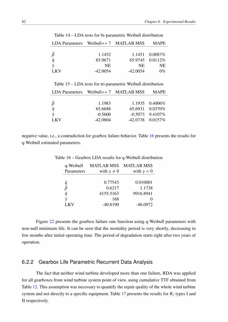
82 Chapter 6. Experimental Results
Table 14 – LDA tests for bi-parametric Weibull distribution
LDA Parameters Weibull++ 7 MATLAB MSS MAPE
β 1.1452 1.1451 0.0087%η 65.9671 65.9745 0.0112%γ NE NE NELKV -42.0054 -42.0054 0%
Table 15 – LDA tests for tri-parametric Weibull distribution
LDA Parameters Weibull++ 7 MATLAB MSS MAPE
β 1.1983 1.1935 0.4006%η 65.6688 65.6931 0.0370%γ -0.5600 -0.5073 9.4107%LKV -42.0804 -42.0738 0.0157%
negative value, i.e., a contradiction for gearbox failure behavior. Table 16 presents the results forq-Weibull estimated parameters.
Table 16 – Gearbox LDA results for q-Weibull distribution
q-Weibull MATLAB MSS MATLAB MSSParameters with γ , 0 with γ = 0
q 0.77543 0.010001β 0.6217 1.1738η 4155.5163 9916.8941γ 168 0LKV -40.8190 -46.0972
Figure 22 presents the gearbox failure rate function using q-Weibull parameters withnon-null minimum life. It can be seen that the mortality period is very shortly, decreasing infew months after initial operating time. The period of degradation starts right after two years ofoperation.
6.2.2 Gearbox Life Parametric Recurrent Data Analysis
The fact that neither wind turbine developed more than one failure, RDA was appliedfor all gearboxes from wind turbine system point of view, using cumulative TTF obtained fromTable 12. This assumption was necessary to quantify the repair quality of the whole wind turbinesystem and not directly to a specific equipment. Table 17 presents the results for R f types I andII respectively.

6.3. Wind Turbine Gearbox Simulation Analysis 83
0 0.5 1 1.5 2 2.5 3 3.5 4 4.5
x 104
0
1
2
3
4
5
6x 10
−3
time (h)
h q(x)
Gearbox q−Weibull Failure Rate Function
Figure 22 – Gearbox failure rate function
Table 17 – Gearbox RDA type I and II results for accumulated TTF data
q-Weibull MATLAB MSS MATLAB MSSParameters R f type I R f type II
β 1.8953 1.907η 5669.1686 6136.7523λ 7.6876e-08 5.9771e-08q f 0.13646 0.41139R f 0.86354 0.58861LKV -46.1825 -45.8908
6.3 Wind Turbine Gearbox Simulation Analysis
6.3.1 Gearbox Life Data Analysis with Non-Perfect Repairs
To study the influence of non-perfect repair in optimum availability for a given asset, it’snecessary first to determine the failure distribution parameters with non-perfect repair effects.This process involves generation of pseudo random TTF vector using the original distributionparameters (Table 16) and applying non-perfect repair formulations (3.2), (3.3), and type I and IIR f values (Table 17) to generate a new set of TTF. To estimate distribution parameters from thenew set of TTF, MLE must be applied according to previously discussed in subsection 6.2.1. Avector of 30 TTF samples was generated to avoid MLE bias effect when using small samples.Table 18 presents the new distribution parameters for restoration types I and II.
84 Chapter 6. Experimental Results
Table 18 – Gearbox LDA results for q-Weibull distribution with non-perfect repairs
q-Weibull Parameters for Parameters for Parameters forParameters original data R f =0.86 type I R f =0.59 type II
q 0.77543 0.85198 0.93098β 0.6217 0.76391 0.81704η 4155.5163 2412.1726 4130.5059γ 168 71.2911 73.9169
6.3.2 Hypothesis Test for Distribution Parameters
The statistical behavior from a set of distribution parameters, subjected to acceleratedlife testing (stress) or maintenance tasks (repairs), can be modified according to the nature ofthese parameters. For example, when applying stress or maintenance repair to bi-parametricWeibull, only the η parameter will change, proportionally to the level of stress or maintenancerepair quality. Otherwise, parameter β will not change due to relationship of that parameter withthe shape of failure, i.e., failure mode. To change β parameter, a resize or project improvementmust be done at the equipment.
To prove if a given distribution parameter changes its statistical properties due to stressor maintenance tasks, a hypothesis tests on the mean must be applied. The null hypothesis H0:
H0 : µθ = µθ0 (6.1)
and alternative hypothesis H1:
H1 :
µθ , µθ0
µθ > µθ0
µθ < µθ0
(6.2)
are the test formulations used to compare between parameters mean µθ0 with TTF for perfectrepair and parameters means from samples with TTF for non-perfect repair µθ. The hypothesistest results obtained are described according to Tables 20 and 21. The test used a significancelevel of 5% (α = 0.05) and a sample size of 20. All samples are normally distributed accord-ing to statistical tests applied (Table 19). The normality condition was obtained applying theAnderson-Darling test, i.e., a statistical test whether a particular data follows a normal distribution(RAZALI; WAH, 2011).
6.3.3 Optimum Availability With Perfect and Non-Perfect Repairs
The optimum calendar preventive maintenance intervals which maximizes the availabilityof gearboxes and hence increase the availability of wind turbine system are obtained applying

6.3. Wind Turbine Gearbox Simulation Analysis 85
Table 19 – Gearbox normality test for parameters distribution type I and II
q-Weibull Anderson-Darling Anderson-DarlingParameter p-value for R f type I p-value for R f type II
q 0.9803 0.4476β 0.5075 0.5965η 0.3594 0.9839γ 0.1261 0.8420
Table 20 – Gearbox hypothesis test for parameters distribution with R f =0.86 type I
q-Weibull µθ µθ0 Hypothesis p-valueParameter test
q 0.77543 0.85198 H0 : µθ < µθ0 0.9781β 0.6217 0.76391 H0 : µθ < µθ0 0.9039η 4155.5163 2412.1726 H0 : µθ > µθ0 0.9822γ 168 71.2911 H0 : µθ > µθ0 0.9633
Table 21 – Gearbox hypothesis test for parameters distribution with R f =0.59 type II
q-Weibull µθ µθ0 Hypothesis p-valueParameter test
q 0.77543 0.93098 H0 : µθ < µθ0 0.9999β 0.6217 0.81704 H0 : µθ < µθ0 0.9995η 4155.5163 4130.5059 H0 : µθ > µθ0 0.5982γ 168 73.9169 H0 : µθ > µθ0 0.9831
equation (4.6) using q-Weibull distributions according to Table 18. The CM and PM repairstimes are constant distributions and was set to Tu = 6Tp, i.e., CM repair is six times longer thenPM repair time. Table 22 presents the optimum calendar PM intervals calculated for perfect andnon-perfect repairs.
Table 22 – Gearbox optimum PM interval for perfect and non-perfect repairs
Repair Optimum PM Tu Tp
type interval t∗d(h)
Perfect repair 21,025 36 6Repair type I 10,300 36 6Repair type II 30,882 36 6
6.3.4 Simulation Results for Perfect and Non-Perfect Models
The asset key performance indicators usually used to evaluated maintenance strategiesapplied are basically the availability and total numbers of correctives and preventives realized
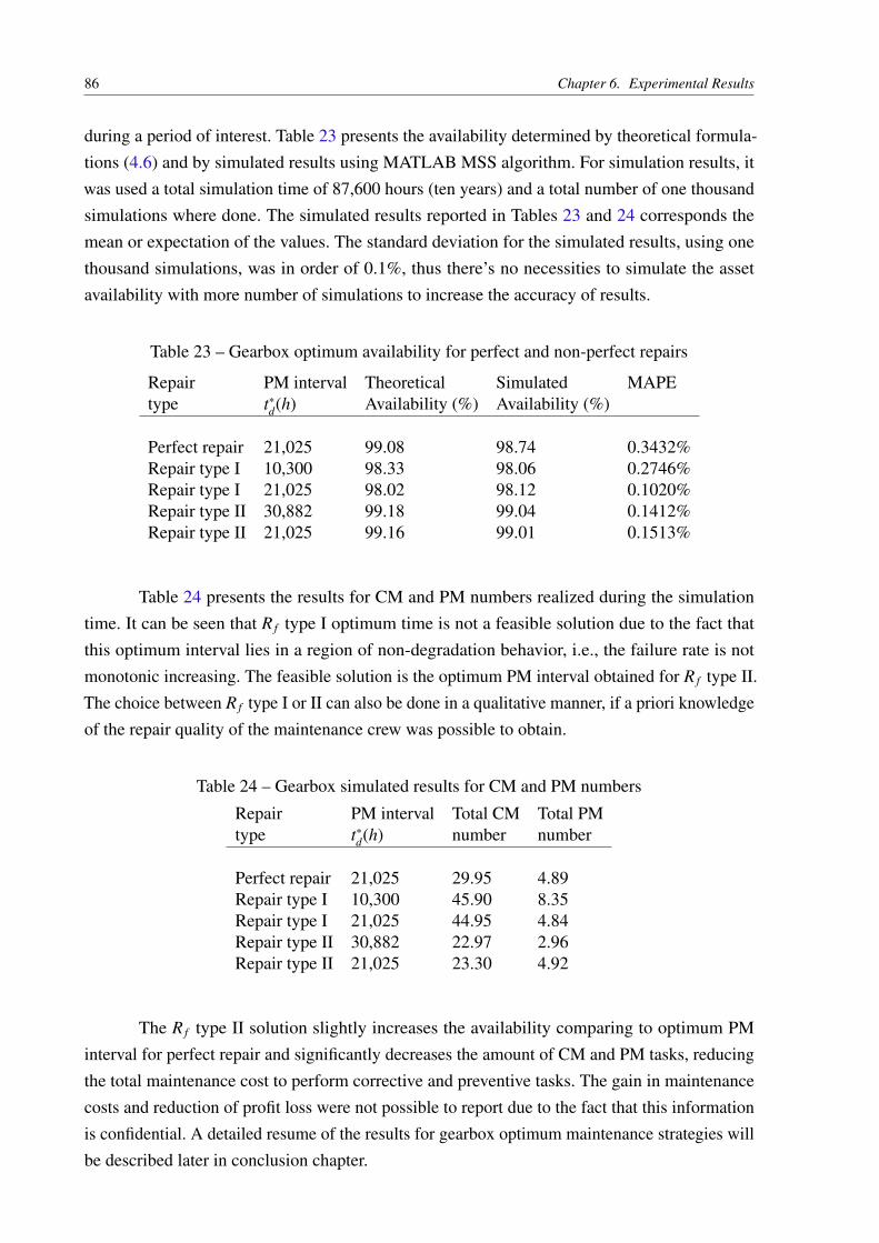
86 Chapter 6. Experimental Results
during a period of interest. Table 23 presents the availability determined by theoretical formula-tions (4.6) and by simulated results using MATLAB MSS algorithm. For simulation results, itwas used a total simulation time of 87,600 hours (ten years) and a total number of one thousandsimulations where done. The simulated results reported in Tables 23 and 24 corresponds themean or expectation of the values. The standard deviation for the simulated results, using onethousand simulations, was in order of 0.1%, thus there’s no necessities to simulate the assetavailability with more number of simulations to increase the accuracy of results.
Table 23 – Gearbox optimum availability for perfect and non-perfect repairs
Repair PM interval Theoretical Simulated MAPEtype t∗d(h) Availability (%) Availability (%)
Perfect repair 21,025 99.08 98.74 0.3432%Repair type I 10,300 98.33 98.06 0.2746%Repair type I 21,025 98.02 98.12 0.1020%Repair type II 30,882 99.18 99.04 0.1412%Repair type II 21,025 99.16 99.01 0.1513%
Table 24 presents the results for CM and PM numbers realized during the simulationtime. It can be seen that R f type I optimum time is not a feasible solution due to the fact thatthis optimum interval lies in a region of non-degradation behavior, i.e., the failure rate is notmonotonic increasing. The feasible solution is the optimum PM interval obtained for R f type II.The choice between R f type I or II can also be done in a qualitative manner, if a priori knowledgeof the repair quality of the maintenance crew was possible to obtain.
Table 24 – Gearbox simulated results for CM and PM numbers
Repair PM interval Total CM Total PMtype t∗d(h) number number
Perfect repair 21,025 29.95 4.89Repair type I 10,300 45.90 8.35Repair type I 21,025 44.95 4.84Repair type II 30,882 22.97 2.96Repair type II 21,025 23.30 4.92
The R f type II solution slightly increases the availability comparing to optimum PMinterval for perfect repair and significantly decreases the amount of CM and PM tasks, reducingthe total maintenance cost to perform corrective and preventive tasks. The gain in maintenancecosts and reduction of profit loss were not possible to report due to the fact that this informationis confidential. A detailed resume of the results for gearbox optimum maintenance strategies willbe described later in conclusion chapter.

6.4. Wind Turbine Electric Fan Motor Case 87
6.4 Wind Turbine Electric Fan Motor Case
An additional case was made to clarify the process done before for the gearbox reliabilityanalysis. This additional case was applied to the electric fan motor of the wind turbine. Thecomplete process to perform the reliability analysis is detailed explained using the Algorithm 4.
Algorithm 4 Reliability analysis process algorithm for electric fan motorInput: TT F vectorOutput: Reliability analysis results
1: TT Faccum. ← Σ(TT F) . Obtain the TTF accumulated values from TTF vector2: Wq(q, β, η, γ)← Λ(xi; θ1, θ2, ..., θk) . Perform LDA for TTF vector using MLE method3: if γ < 0 then4: Wq(q, β, η, 0)← Λ(xi; θ1, θ2, ..., θk) . Perform LDA with γ = 0 to avoid negative values5: end if6: R ftype−I ,R ftype−II ← RDA(TT Faccum.) . Calculates R f values for RDA types I and II7: TT Ftype−I ,TT Ftype−II ← Wq(q, β, η, γ) . Generates TTF vectors with non-repair effects
types I and II8: Wqtype−I (q, β, η, γ),Wqtype−II (q, β, η, γ)← Λ(xi; θ1, θ2, ..., θk) . Perform LDA for TTF vectors
with non-repair effects types I and II9: Tu,Tp . Determine the values for corrective and preventive repair times
10: t∗dtype−I, t∗dtype−II
← min fd(t) . Calculates optimum calendar downtime-based PM intervals forR f types I and II
11: tsim . Determine the simulation total time12: nsim . Calculate the number of simulation runs according to (5.2)13: MS S (tsim, nsim,Wq, ...,Tu,Tp) . Perform the simulation using MATLAB MSS algorithm
for R f types I and II scenarios14: Atheo.(t), Asim.(t), EM . Perform analysis for theoretical and simulated availability values.
Evaluate the EM error15: #CM, #PM . Perform analysis for numbers of corrective and preventive maintenance
Table 25 presents the estimated parameters for q-Weibull distribution obtained fromoriginal TTF data and TTF vector generated with non-perfect repair effects. The original TTFdata was obtained from the computerized maintenance management system (CMMS) databaseduring a period of the last two years. It can be seen that all the q-Weibull estimated parameterslie in a failure rate region with monotonically increasing, thus, the preventive maintenance isjustified. The γ parameters were set to zero due to negative values obtained by MLE method.
Table 25 – Electric fan motor LDA results for q-Weibull distribution parameters
q-Weibull Parameters for Parameters for Parameters forParameters original data R f =0.9990 type I R f =0.9983 type II
q 0.0100 0.1801 0.0113β 4.3829 4.5119 5.6404η 746.0171 657.1377 726.5341γ 0.0000 0.0000 0.0000

88 Chapter 6. Experimental Results
Table 26 presents the optimal calendar downtime PM interval values for perfect andnon-perfect repair calculated according to (4.6). The CM and PM repairs times are the sameused for gearbox case.
Table 26 – Electric fan motor optimum PM interval for perfect and non-perfect repairs
Repair Optimum PM Tu Tp
type interval t∗d(h)
Perfect repair 317.094 36 6Repair type I 289.644 36 6Repair type II 354.115 36 6
The theoretical and simulated availability values for perfect and non-perfect repairs arepresented by Table 27. The MAPE evaluated either for gearbox (Table 23) and electric fan motor(Table 27) were low, around 1%. The simulation parameters used in MATLAB MSS algorithmwere: 8,760 hours (one year) for total simulation time, and one thousand simulations runs.
Table 27 – Electric fan motor optimum availability for perfect and non-perfect repairs
Repair PM interval Theoretical Simulated MAPEtype t∗d(h) Availability (%) Availability (%)
Perfect repair 317.094 97.62 96.91 0.73%Repair type I 289.644 97.42 96.46 0.99%Repair type I 317.094 97.37 96.34 1.06%Repair type II 354.115 97.99 97.43 0.57%Repair type II 317.094 97.94 97.58 0.37%
Table 28 presents the simulated results for CM and PM numbers. As it can be seen, dueto the fact that R f values for both types I and II are closer to perfect repair (R f = 1), the gain inavailability and corrective maintenance by using PM interval for type II was slight.
Table 28 – Electric fan motor simulated results for CM and PM numbers
Repair PM interval Total CM Total PMtype t∗d(h) number number
Perfect repair 317.094 3.84 22.16Repair type I 289.644 4.73 23.34Repair type I 317.094 5.59 19.98Repair type II 354.115 2.76 21.05Repair type II 317.094 1.66 25.38

89
7 Conclusion
The onshore wind turbine case applied in this work made possible to apply all theconcepts studied in this master thesis. As mentioned before, the correct choices for maintenancetask types along with the optimized intervals, represents the optimum maintenance policies whichdrives a given asset to perform optimum levels of availability and thus ensure the production,reliability and operational safety results.
The availability measures calculated in this practical case is a common metric for measureasset operational results at many industrial contexts. The analysis and optimizations made wasstrategic to guarantee the safe and profitable asset operation. The asset life cycle studied isdynamic and can be influenced by industrial operational context, maintenance policies andquality of repair. The q-Weibull distribution applied in this work has the flexibility to model theentire asset life cycle, allowing to assign different maintenance strategies for any asset life phase.
The life data analysis performed using the gearbox wind turbine database, can show thatthe asset performed the entire bathtub curve along its life period. The premature failure periodstarts at the beginning of operation and extends to approximately six months. The useful lifeperiod was approximately 10 thousand hours, after that, the wearout period begins.
The parametric recurrent data analysis, made for the wind turbine system using thecumulative time to failure database, presented different quality of repair when using type I andtype II GRP models. This different values are justified due to the fact that type II restorationeliminates all past imperfect repairs, thus, the restoration factor must be lower than type I.
The hypothesis test was made to proof that repairs did not affect the failure rate shape forWeibull and q-Weibull distributions. As can be seen with the results obtained using hypothesistest, when using q-Weibull, the failure rate shape, which is function of parameters q and β, didnot modify the original failure rate shape even with these parameters changed after non-perfectrepairs. For Weibull distribution, the failure rate shape is modeled only by parameter β, whichremains statistically constant when applied the hypothesis test for time to failure data using non-perfect repairs. The U-shaped or bathtub curve remains the same for new q-Weibull distributionswith non-perfect repairs.
The optimum preventive calendar interval, which maximizes the gearbox availability,was calculated for perfect and non-perfect repairs (type I and II models). The theoretical resultsobtained shows that the gain in availability, if applied the optimum interval for all 72 windturbines, was in order of 22% for type I and 1.44% for type II. The simulated results for thetotal number of corrective and preventive maintenance realized during the entire simulation time,shows that type I presented an increase of 0.95 failures for CM and 3.51 failures for PM, whiletype II, presented a decrease of 0.33 failures for CM and 1.96 failures for PM.

90 Chapter 7. Conclusion
Basically, the presented results show that type I model is an unfeasible solution due tothe fact that the optimum interval of 10,300 hours lies in a region of constant failure rate whichis not recommended for PM strategies. The choice for type II optimum interval of 30,882 hoursgives an increment in availability and reduces both number of CM and PM maintenance whencompared with the optimum interval of 21,025 hours.
Improvements and future studies proposed for this work are regarding to the analysis ofoptimum grouped preventive intervals for non-perfect repair using different failure modes forequipments and components of the wind turbine. Besides, the development of models for opti-mum predictive intervals also with non-perfect repairs and inclusion of predictive maintenancemodule into the MATLAB MSS algorithm.

91
Bibliography
ABRAMOWITZ, M.; STEGUN, I. A. Handbook of Mathematical Functions with Formulas,Graphs and Mathematical Tables. 1. ed. New York, USA: Dover Publications, Inc., 1968.1045 p.
ARORA, J. S. Introduction to Optimum Design. 3. ed. Waltham, MA, USA: Elsevier, 2012.880 p.
ASSIS, E. M.; BORGES, E. P.; MELO, S. A. B. V. Generalized q-weibull model and the bathtubcurve. International Journal of Quality Reliability Management, v. 1, n. 30, p. 19, 2013.
ASSIS, E. M. de. O Modelo q-Weibull em Confiabilidade, Árvores de Falha Dinâmicas eImplementação de Manutenção. Tese (Doutorado) — Universidade Federal da Bahia - EscolaPolitécnica, Salvador, julho 2013.
BARLOW, R.; HUNTER, L. Optimum preventive maintenance policies. Operations Research,v. 8, n. NE, p. 90–100, 1960.
BARLOW, R. E. Engineering Reliability. 1. ed. Philadelphia, USA: ASA-SIAM, 1998. 199 p.
BAZOVSKY, I. Reliability Theory and Practice. 1. ed. Mineola, New York, USA: DoverPublications, Inc., 2004. 292 p.
BIROLINI, A. Reliability Engineering - Theory and Practice. 5. ed. London, UK: Springer,2007. 593 p.
BLOOM, N. B. Reliability Centered Maintenance: Implementation made simple. 1. ed. NewYork, USA: McGraw-Hill Books, 2005. 291 p.
BOYD, S.; VANDENBERGHE, L. Convex Optimization. 7. ed. The Edinburgh Building,Cambridge, CB2 8RU, UK: Cambridge University Press, 2009. 716 p.
BROWN, R. E. Electric Power Distribution Reliability. 1. ed. New York, USA: Marcel Dekker,Inc., 2002. 380 p.
CÂMARA DE COMERCIALIZAÇÃO DE ENERGIA ELÉTRICA. CCEE: Regras decomercialização - garantia física. Brazil, 2016. 73 p.
CÂMARA DE COMERCIALIZAÇÃO DE ENERGIA ELÉTRICA. CCEE: Regras decomercialização - medição contábil. Brazil, 2017. 129 p.
CASSADY, C. R. et al. A generic model of equipment availability under imperfect maintenance.IEEE Transactions on Reliability, v. 54, n. 4, p. 564–571, 2005.
CHAN, W. K. Theory and Applications of Monte Carlo Simulations. 1. ed. RensselaerPolytechnic Institute, USA: InTech, 2013. 284 p.
CHEN, F. et al. Research on imperfect preventive maintenance strategy for turret system of thecnc lathe. 11th International Conference on Reliability, Maintainability and Safety (ICRMS),NE, n. NE, p. 1–4, 2016.

92 Bibliography
CHUNG, H. S. hung et al. Reliability of Power Electronic Converter Systems. 1. ed. London,UK: The Institution of Engineering and Technology, 2016. 489 p.
COSTA, U. M. S. et al. An improved description of the dielectric breakdown in oxides based ona generalized weibull distribution. Physica A, v. 1, n. 361, p. 209–2015, 2006.
DEPARTMENT OF DEFENSE - DOD. MIL-STD-3034: Reliability-centered maintenance (rcm)process. USA, 2011. 64 p.
DHILLON, B. S. Maintainability, Maintenance and Reliability for Engineers. 1. ed. Florida,USA: Taylor & Francis Group, 2006. 214 p.
EBELING, C. E. An Introduction to Reliability and Maintainability Engineering. 1. ed. NewYork, USA: The McGraw-Hill Companied, Inc., 1997. 486 p.
FINKELSTEIN, M. Failure Rate Modelling for Reliability and Risk. 1. ed. London, UK:Springer, 2008. 290 p.
FITCH, E. C. Proactive Maintenance for Mechanical Systems. 1. ed. Oklahoma, USA: Elsevier,1992. 337 p.
GNEDENKO, B.; USHAKOV, I. Probabilistic Reliability Engineering. 1. ed. New York, USA:John Wiley & Sons, Inc., 1995. 518 p.
GOTI, A. Discrete Event Simulations. 1. ed. Rijeka, Croatia: Sciyo, 2010. 330 p.
GUO, H. et al. Piecewise nhpp models with maximum likelihood estimation for repairablesystems. IEEE Annual Reliability and Maintainability Symposium, 2010. Proceedings, NE,n. NE, p. 7, 2010.
GUO, H.; ZHAO, W.; METTAS, A. Practical methods for modeling repairable systems withtime trends and repair effects. IEEE Annual Reliability and Maintainability Symposium, 2006.Proceedings, NE, n. NE, p. 7, 2006.
GUO, H. R. et al. A new stochastic model for systems under general repairs. IEEE Transactionson Reliability, v. 56, n. 1, p. 10, 2007.
INTERNATIONAL ORGANIZATION FOR STANDARDIZATION. ISO 9000-4 :1993, Qualitymanagement and quality assurance standards — Part 4: Guide to dependability programmemanagement. EUA, 1993.
JARDINE, A. K. S. Maintenance, Replacement and Reliability. 1. ed. Ontario, Canada: PitmanPublishing, 1973. 199 p.
JARDINE, A. K. S.; TSANG, A. H. C. Maintenance, Replacement and Reliability - Theory andApplications. 2. ed. Boca Raton, FL, USA: CRC Press, 2013. 330 p.
KARKI, R.; BILLINTON, R.; VERMA, A. K. Reliability Modeling and Analysis of SmartPower Systems. 1. ed. New Delhi, India: Springer India, 2014. 202 p.
KECECIOGLU, D. B. Reliability & Life Testing Handbook - Volume 1. 1. ed. Lancaster,Pennsylvania, USA: DEStech Publications, 2002. 803 p.
KECECIOGLU, D. B. Reliability & Life Testing Handbook - Volume 2. 1. ed. Lancaster,Pennsylvania, USA: DEStech Publications, 2002. 793 p.
Bibliography 93
KIJIMA, M. Some results for repairable systems with general repair. Journal of AppliedProbability, v. 26, n. 1, p. 89–102, 1989.
KIJIMA, M.; SUMITA, U. A useful generalization of renewal theory: Counting processesgoverned by non-negative markovian increments. Journal of Applied Probability, v. 23, n. 1, p.71–88, 1986.
KLINGER, D. J.; NAKADA, Y.; MENENDEZ, M. A. AT&T Reliability Manual. 1. ed. NewYork, USA: Van Nostrand Reinhold, 1990. 225 p.
KROESE, D. P.; TAIMRE, T.; BOTEV, Z. I. Handbook of Monte Carlo Methods. 1. ed. Hoboken,New Jersey, USA: John Wiley & Sons Ltd., 2011. 743 p.
LISBOA, A. C. et al. Planejamento de manutenções para minimização do impacto do mecanismode redução de garantia física. XXIII SNPTEE - Seminário Nacional de Produção e Transmissãode Energia Elétrica, v. 1, n. 23, p. 9, 2015.
LIU, Y.; HUANG, H. Z. Optimal selective maintenance strategy for multi-state systems underimperfect maintenance. IEEE Transactions on Reliability, v. 59, n. 2, p. 356–367, 2010.
LU, X. et al. Exact results on the statistically expected total cost and optimal solutions forextended periodic imperfect preventive maintenance. IEEE Transactions on Reliability, v. 61,n. 2, p. 378–388, 2012.
MATHWORKS. MATLAB: Optimization toolbox user’s guide - version 2. Natick, MA, USA,2003. 352 p.
MEEKER, W. Q.; ESCOBAR, L. A. Statistical Methods for Reliability Data. 1. ed. New York,USA: John Wiley & Sons Ltd., 1998. 680 p.
METTAS, A.; ZHAO, W. Modeling and analysis of repairable systems with general repair. IEEEAnnual Reliability and Maintainability Symposium, 2005. Proceedings, NE, n. NE, p. 7, 2005.
MOBLEY, R. K. An Introduction to Predictive Maintenance. 2. ed. Woburn, MA, USA:Butterworth-Heinemann Ltd, 2002. 438 p.
MONTGOMERY, D. C.; RUNGER, G. C. Applied Statistics and Probability for Engineers. 5.ed. New York, USA: John Wiley & Sons, Inc., 2011. 768 p.
MOUBRAY, J. Reliability-centred Maintenance (RCM). 1. ed. Oxford, UK: Butterworth-Heinemann Ltd, 1994. 320 p.
NELSON, W. B. Applied Life Data Analysis. 1. ed. New York, USA: John Wiley & Sons Ltd.,1982. 634 p.
O’CONNOR, A. N. Probability Distributions Used in Reliability Engineering. 1. ed. CollegePark, Maryland, USA: University of Maryland, 2011. 208 p.
O’CONNOR, P. D. T.; KLEYNER, A. Practical Reliability Engineering. 5. ed. New York, USA:John Wiley & Sons Ltd., 2012. 484 p.
PATTON, J. D. Maintainability and Maintenance Management. 1. ed. North Carolina, USA:Instrument Society of America, 1980. 441 p.

94 Bibliography
PHAM, H. Handbook of Reliability Engineering. 1. ed. London, UK: Springer-Verlag, 2003.663 p.
PICOLI, S.; MENDES, R. S.; MALACARNE, L. C. q-exponential, weibull, and q-weibulldistributions: An empirical analysis. Physica A, v. 1, n. 324, p. 678–688, 2003.
PRESS, W. H. et al. Numerical Recipes in C - The Art of Scientific Computing. 3. ed. New York,USA: Cambridge University Press, 2007. 1235 p.
RAZALI, N. M.; WAH, Y. B. Power comparisons of shapiro-wilk, kolmogorov-smirnov,lilliefors and anderson-darling tests. Journal of Statistical Modeling and Analytics, v. 2, n. 1, p.21–33, 2011.
RELIASOFT CORPORATION. RCM++: Rcm - user’s guide. Tucson, Arizona, USA, 2005.632 p.
RELIASOFT CORPORATION. Weibull++ 7: Life data analysis reference. Tucson, Arizona,USA, 2005. 580 p.
RELIASOFT CORPORATION. BlockSim 7: System analysis reference - reliability, availability& optimization. Tucson, Arizona, USA, 2007. 487 p.
RELIASOFT CORPORATION. RGA: Reliability growth & repairable system data analysisreference. Tucson, Arizona, USA, 2009. 587 p.
SILVA, G. C. et al. Advanced fuzzy time series applied to short term load forecasting. 4th IEEELatin American Conference on Computational Intelligence, NE, n. NE, p. 6, 2017.
SILVA, J. L. R. Caracterização de equipes de manutenção com base nos parâmetros dadistribuição weibull obtidos pela maximização da mle utilizando o algoritmo elipsoidal. 30o
Congresso Brasileiro de Manutenção e Gestão de Ativos, NE, n. NE, p. 10, 2015.
SILVA, J. L. R. Determinação dos parâmetros da distribuição weibull obtidos pela maximizaçãoda mle utilizando o algoritmo elipsoidal. 13o Simpósio Internacional de Confiabilidade, NE,n. NE, p. 8, 2015.
SILVA, J. L. R. Optimum preventive maintenance strategies using electre i multicriteriadecision-making method. ABRISCO 2015 - Congresso da Associação Brasileira de Análise deRisco, Segurança de Processo e Confiabilidade, NE, n. NE, p. 8, 2015.
SILVA, J. L. R. et al. Forecasting wind turbines failure data using advanced fuzzy time series.ABRISCO 2017 - Congresso da Associação Brasileira de Análise de Risco, Segurança deProcesso e Confiabilidade, NE, n. NE, p. 5, 2017.
SILVA, J. L. R.; LISBOA, A. C.; SALDANHA, R. R. Forecasting power quality events usingadvanced fuzzy time series. XII Conferência Brasileira sobre Qualidade de Energia Elétrica,NE, n. NE, p. 6, 2017.
SILVA, J. L. R.; SALDANHA, R. R. Utilização do algoritmo elipsoidal para caracterização deequipes de reparo de manutenção e correlação com parâmetros de qualidade da energia. XIConferência Brasileira sobre Qualidade de Energia Elétrica, NE, n. NE, p. 8, 2015.
SILVA, J. L. R.; SALDANHA, R. R.; LISBOA, A. C. Abordagem multiobjetiva para otimizaçãode estratégias de manutenção utilizando a distribuição q-weibull. 15o Simpósio Internacional deConfiabilidade, NE, n. NE, p. 5, 2017.

Bibliography 95
SILVA, J. L. R.; SALDANHA, R. R.; LISBOA, A. C. Otimização de intervalos de manutençãopreditiva - estudo de caso para análise de Óleo lubrificante em plantas industriais. 32o CongressoBrasileiro de Manutenção e Gestão de Ativos, NE, n. NE, p. 11, 2017.
SMITH, A. M.; HINCHCLIFFE, G. R. RCM - Gateway to World Class Maintenance. 1. ed.Oxford, UK: Elsevier, 2003. 336 p.
SMOLA, A.; VISHWANATHAN, S. V. N. Introduction to Machine Learning. 1. ed. Cambridge,UK: Cambridge University Press, 2008. 226 p.
TAVNER, P. Offshore Wind Turbines - Reliability, Availability and Maintenance. 1. ed. London,UK: The Institution of Engineering and Technology, 2012. 269 p.
THE INSTITUTE OF ELECTRICAL AND ELECTRONICS ENGINEERS - IEEE. IEEE Std493-1997: Recommended practice for the design of reliable industrial and commercial powersystems. New York, USA, 2007. 369 p.
THE INSTITUTE OF ELECTRICAL AND ELECTRONICS ENGINEERS - IEEE. IEEE Std1366-2012: Guide for electric power distribution reliability indices. New York, USA, 2012. 40 p.
U.S DEPARTMENT OF ENERGY - FEDERAL ENERGY MANAGEMENT PROGRAM(FEMP). Operations & Maintenance Best Practices: A guide to achieving operational efficiency.USA, 2010. 321 p.
USHAKOV, I. A.; HARRISON, R. A. Handbook of Reliability Engineering. 1. ed. New York,USA: John Wiley & Sons, Inc., 1994. 663 p.
VIANA, H. R. G. Planejamento e Controle da Manutenção. 1. ed. Rio de Janeiro, Brasil:Qualitymark Editora Ltda., 2006. 192 p.
WANG, H.; PHAM, H. Reliability and Optimal Maintenance. 1. ed. London, UK:Springer-Verlag, 2006. 345 p.
XUA, M. et al. On the q-weibull distribution for reliability applications: An adaptive hybridartificial bee colony algorithm for parameter estimation. Reliability Engineering and SystemSafety, v. 1, n. 158, p. 93–105, 2017.
YANG, G. Life Cycle Reliability Engineering. 1. ed. New York, USA: John Wiley & Sons, Inc.,2007. 517 p.
ZIO, E. An Introduction to the Basics of Reliability and Risk Analysis. 1. ed. 5 Toh Tuck Link,Singapore: World Scientific Publishing Co. Re. Ltd., 2007. 222 p.