optimization methods for ndp - wayne state universityhzhang/courses/7290b/lectures/05... ·...

Optimization Methods for NDP

Acknowledgment: the slides are based on those from Drs. Yong Liu, Deep Medhi, and Michał Pióro.

Hongwei Zhang

http://www.cs.wayne.edu/~hzhang

Optimization Methods

optimization -- choose the “best”. what “best” means -- objective function what choices you have -- feasible set

solution methods brute-force, analytical, and heuristic solutions linear/integer/convex programming

Outline

Linear programming Integer/mixed integer programming NP-Completeness Branch-Bound

LP decomposition methods Stochastic heuristics Matlab optimization toolbox

Outline


LP decomposition methods Matlab optimization toolbox Stochastic heuristics

Linear Programming - a problem and its solution

maximize z = x1 + 3x2 subject to - x1 + x2 ≤ 1

x1 + x2 ≤ 2

x1 ≥ 0 , x2 ≥ 0

x2

x1

-x1+x2 =1

x1+x2 =2

x1+3x2 =z

z=5

z=3

z=0

(1/2,3/2)

Extreme point (vertex): a feasible point that cannot be expressed as a convex linear combination of other feasible points.

Linear Program in Standard Form indices

j=1,2,...,n variables i=1,2,...,m equality constraints

constants c = (c1,c2,...,cn) cost coefficients b = (b1,b2,...,bm) constraint right-hand-sides A = (aij) m × n matrix of constraint coefficients

variables x = (x1, x2,...,xn)

Linear program maximize z = Σj=1,2,...,n cjxj subject to Σj=1,2,...,m aijxj = bi , i=1,2,...,m xj ≥ 0 , j=1,2,...,n

Linear program (matrix form) maximize cx subject to Ax = b x ≥ 0

n > m rank(A) = m

SIMPLEX

Transformation of LPs to the standard form

Inequalities: slack variables Σj=1,2,...,m aijxj ≤ bi to Σj=1,2,...,m aijxj + xn+i = bi , xn+i ≥ 0

Σj=1,2,...,m aijxj ≥ bi to Σj=1,2,...,m aijxj - xn+i = bi , xn+i ≥ 0

Unconstrained sign: diff. between two nonnegative variables

xk with unconstrained sign: xk = xk′ - xk

″ , xk′ ≥ 0 , xk

″ ≥ 0

Exercise: transform the following LP to the standard form maximize z = x1 + x2

subject to 2x1 + 3x2 ≤ 6

x1 + 7x2 ≥ 4

x1 + x2 = 3 x1 ≥ 0 , x2 unconstrained in sign

Basic facts of Linear Programming feasible solution - satisfying constraints basis matrix - a non-singular m × m submatrix of A basic solution to a LP - the unique vector determined by a basis

matrix: n-m variables associated with columns of A not in the basis matrix are set to 0, and the remaining m variables result from the square system of equations

basic feasible solution - basic solution with all variables nonnegative (at most m variables can be positive)

Theorem 1. The objective function, z, assumes its maximum at an

extreme point of the constraint set. Theorem 2. A vector x = (x1, x2,...,xn) is an extreme point of the

constraint set if and only if x is a basic feasible solution.

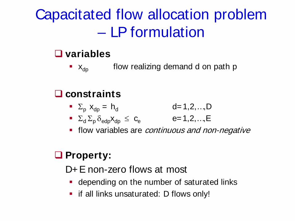
Capacitated flow allocation problem – LP formulation

variables xdp flow realizing demand d on path p

constraints

Σp xdp = hd d=1,2,…,D Σd Σp δedpxdp ≤ ce e=1,2,…,E flow variables are continuous and non-negative

Property: D+E non-zero flows at most

depending on the number of saturated links if all links unsaturated: D flows only!

Solution Methods for Linear Programs (1)

cT

x1

x2

Simplex Method Optimum must be at

the intersection of constraints

Intersections are easy to find, change inequalities to equalities

Jump from one vertex to another

Efficient solution for most problems, exponential time worst case.

Interior Point Methods (IPM) Instead of considering only

vertices of the solution polytope by moving along its edges, IPM follow a path through the interior of the polgytope

Benefits Scales Better than Simplex Certificate of Optimality

cT

x1

x2

Solution Methods for Linear Programs (2)

Outline



IPs and MIPs

Integer Program (IP) maximize z = cx subject to Ax ≤ b, x ≥ 0 (linear constraints) x integer (integrality constraint)

Mixed Integer Program (MIP)

maximize z = cx + dy subject to Ax + Dy ≤ b, x, y ≥ 0 (linear constraints) x integer (integrality constraint)

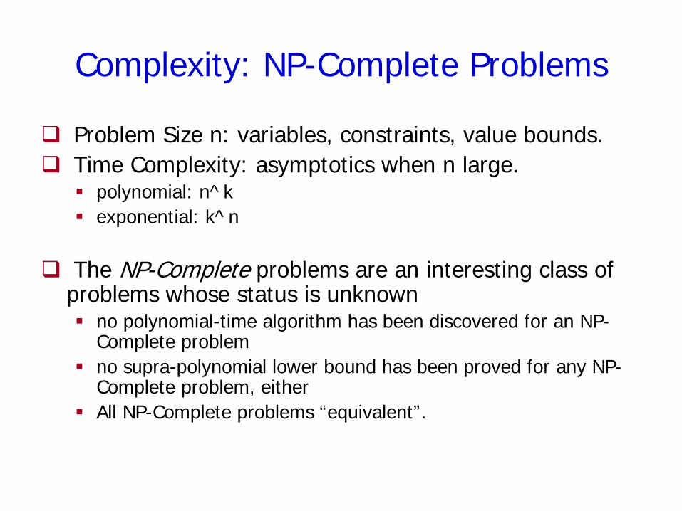
Complexity: NP-Complete Problems

Problem Size n: variables, constraints, value bounds. Time Complexity: asymptotics when n large.

polynomial: n^k exponential: k^n

The NP-Complete problems are an interesting class of

problems whose status is unknown no polynomial-time algorithm has been discovered for an NP-

Complete problem no supra-polynomial lower bound has been proved for any NP-

Complete problem, either All NP-Complete problems “equivalent”.

Prove NP-Completeness

Why? most people accept that it is probably intractable don’t need to come up with an efficient algorithm can instead work on approximation algorithms

How? reduce (transform) a well-known NP-Complete

problem P into your own problem Q if P reduces to Q, P is “no harder to solve” than Q

IP (and MIP) is NP-Complete

SATISFIABILTY PROBLEM (SAT) can be expressed as

IP even as a binary program (all integer variables are

binary)

SATISFIABILITY PROBLEM SAT U = {u1,u2,…um} - Boolean variables; t : U → {true, false} - truth assignment a clause - {u1,u2,u4 } represents conjunction of its elements (u1 + u2 + u4) a clause is satisfied by a truth assignment t if and only if one of its elements is true

under assignment t C - finite collection of n clauses SAT: given: a set U of variables and a collection C of clauses question: is there a truth assignment satisfying all clauses in C?

So far there are several thousands of known NP problems, (including Travelling Salesman, Clique, Steiner Problem, Graph Colourability, Knapsack) to which SAT can be reduced

SAT is NP-complete (Cook’s theorem)

X - set of vectors x = (x1,x2,...,xn) x ∈ X iff Ax ≤ b and x are integers Decision problem: Instance: given n, A, b, C, and linear function f(x). Question: is there x ∈ X such that f(x) ≤ C? The SAT problem is directly reducible to a binary IP problem. assign binary variables xi and xi with each Boolean variables ui and

ui

an inequality for each clause of the instance of SAT (x1 + x2 + x4 ≥ 1)

add inequalities: 0 ≤ xi ≤ 1, 0 ≤ xi ≤ 1, 1 ≤ xi + xi ≤ 1, i=1,2,...,n

Integer Programming is NP-Complete

Optimization Methods for MIP and IP

no hope for efficient (polynomial time) exact general methods

main stream for achieving exact solutions: branch-and-bound

based on LP

• can be enhanced with Lagrangian relaxation

a variant: branch-and-cut

stochastic heuristics

evolutionary algorithms, simulated annenaling, etc.

Why LPs, MIPs, and IPs are so Important?

in practice only LP guarantees efficient solutions decomposition methods are available for LPs

MIPs and IPs can be solved by general solvers using the

branch-and-cut method, based on LP sometimes very efficiently

otherwise, we have to use (frequently) unreliable stochastic meta-heuristics (sometimes specialized heuristics)

Enumeration – Tree Search, Dynamic Programming etc.

Guaranteed to find a feasible solution (only consider integers, can check feasibility (P) )

But, exponential growth in computation time

Solution Methods for Integer Programs

x1=0

X2=0 X2=2 X2=1

x1=1 x1=2

X2=0 X2=2 X2=1 X2=0 X2=2 X2=1


How about solving LP Relaxation followed by rounding?

-cT

x1

x2

LP Solution

Integer Solution

Integer Programs

LP solution provides lower bound on IP But, rounding can be arbitrarily far away from integer

solution

-cT

x1

x2

Combined approach to Integer Programming

-cT

x1

x2

-cT

x1

x2

Why not combine both approaches! Solve LP Relaxation to get fractional solutions Create two sub-branches by adding constraints

x2≤1

x2≥2

Known as Branch and Bound Branch as above For minimizing problem, LP give lower bound, feasible

solutions give upper bound


LP

J* = J0

LP + x1≥4

J* = J2

LP + x1≤3

J* = J1

x1= 3.4, x2= 2.3

LP + x1≤3, x2≤2

J* = J3

LP + x1≤3, x2≥3

J* = J4

LP + x1≥4, x2≥4

J* = J6

LP + x1 ≥ 4, x2 ≤ 3

J* = J5

x1= 4, x2= 3.7 x1= 3, x2= 2.6

Branch and Bound Method for Integer Programs

Branch and Bound Algorithm

1. Solve LP relaxation for lower bound on cost for current branch

• If solution exceeds upper bound, branch is terminated

• If solution is integer, replace upper bound on cost

2. Create two branched problems by adding constraints to original

problem

• Select integer variable with fractional LP solution

• Add integer constraints to the original LP

3. Repeat until no branches remain, return optimal solution.

Additional Refinements – Cutting Planes

Idea stems from adding additional constraints to LP to improve tightness of relaxation

Combine constraints to eliminate non-integer solutions

x1

x2

Added Cut

All feasible integer solutions remain feasible

Current LP solution is not feasible

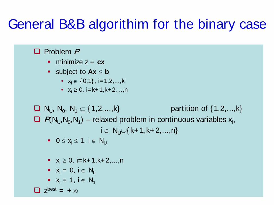
General B&B algorithim for the binary case

Problem P minimize z = cx subject to Ax ≤ b

• xi ∈ {0,1}, i=1,2,...,k • xi ≥ 0, i=k+1,k+2,...,n

NU, N0, N1 ⊆ {1,2,...,k} partition of {1,2,...,k} P(NU,N0,N1) – relaxed problem in continuous variables xi, i ∈ NU∪{k+1,k+2,...,n}

0 ≤ xi ≤ 1, i ∈ NU

xi ≥ 0, i=k+1,k+2,...,n xi = 0, i ∈ N0

xi = 1, i ∈ N1

zbest = +∞

B&B for the binary case - algorithm

procedure BBB(NU,N0,N1) begin solution(NU,N0,N1,x,z); { solve P(NU,N0,N1) } if NU = ∅ or for all i ∈ NU xi are binary then if z < zbest then begin zbest := z; xbest := x end else if z ≥ zbest then return { bounding } else begin { branching } choose i ∈ NU such that xi is fractional; BBB(NU \ { i },N0∪ { i },N1); BBB(NU \ { i },N0,N1∪ { i }) end end { procedure }

original problem: (IP) maximize cx subject to Ax ≤ b x ≥ 0 and integer linear relaxation: (LR) maximize cx subject to Ax ≤ b x ≥ 0

B&B - example

The optimal objective value for

(LR) is greater than or equal to the

optimal objective for (IP).

If (LR) is infeasible then so is (IP).

If (LR) is optimised by integer

variables, then that solution is

feasible and optimal for (IP).

If the cost coefficients c are

integer, then the optimal objective

for (IP) is less than or equal to the

“round down” of the optimal

objective for (LR).

B&B - knapsack problem maximize 8x1 + 11x2 + 6x3+ 4x4 subject to 5x1 + 7x2 + 4x3 + 3x4 ≤ 14

xj ∈ {0,1} , j=1,2,3,4

(LR) solution: x1 = 1, x2 = 1, x3 = 0.5, x4 = 0, z = 22 no integer solution will have value greater than 22

Fractional z = 22

x3 = 0 Fractional z = 21.65


add the constraint to (LR)

x1 = 1, x2 = 1, x3 = 0, x4 = 0.667 x1 = 1, x2 = 0.714, x3 = 1, x4 = 0

we know that the optimal integer solution is not greater than 21.85 (21 in fact) we will take a subproblem and branch on one of its variables

- we choose an active subproblem (here: not chosen before) - we choose a subproblem with highest solution value

B&B example cntd.

Fractional z = 22



x1 = 1, x2 = 0, x3 = 1, x4 = 1 x1 = 0.6, x2 = 1, x3 = 1, x4 = 0

x3 = 1, x2 = 0 Integer z = 18 INTEGER

x3 = 1, x2 = 1 Fractional z = 21.8

no further branching, not active

B&B example cntd. Fractional z = 22



x1 = 0, x2 = 1, x3 = 1, x4 = 1 x1 = 1, x2 = 1, x3 = 1, x4 = ?

x3 = 1, x2 = 0 Integer z = 18 INTEGER

x3 = 1, x2 = 1 Fractional z = 21.8

x3 = 1, x2 = 1, x1 = 0 Integer z = 21 INTEGER

x3 = 1, x2 = 1, x1 = 1 Infeasible INFEASIBLE

there is no better solution than 21: bounding

optimal

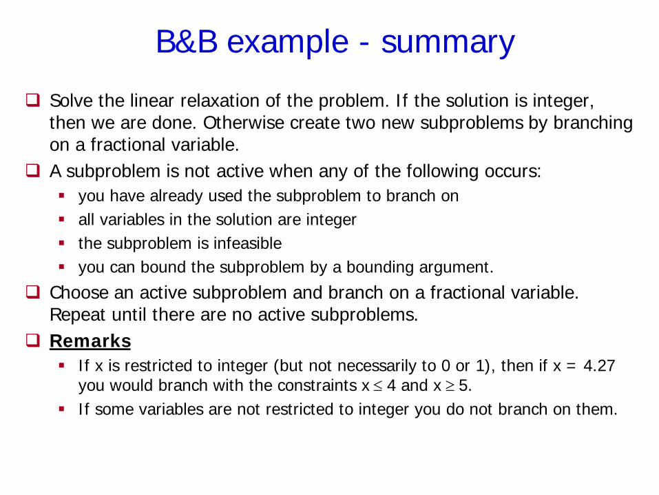
B&B example - summary

Solve the linear relaxation of the problem. If the solution is integer, then we are done. Otherwise create two new subproblems by branching on a fractional variable.

A subproblem is not active when any of the following occurs: you have already used the subproblem to branch on all variables in the solution are integer the subproblem is infeasible you can bound the subproblem by a bounding argument.

Choose an active subproblem and branch on a fractional variable. Repeat until there are no active subproblems.

Remarks If x is restricted to integer (but not necessarily to 0 or 1), then if x = 4.27

you would branch with the constraints x ≤ 4 and x ≥ 5. If some variables are not restricted to integer you do not branch on them.

B&B algorithim - comments

Also, integer MIP can always be converted into binary MIP transformation: xj = 20uj0 + 21uj1 + ... + 2qujq (xj ≤ 2q+1 -1)

Lagrangian relaxation can also be used for finding lower bounds (instead of linear relaxation).

Branch-and-Cut (B&C) combination of B&B with the cutting plane method

• the most effective exact approach to NP-complete MIPs

idea: add ”valid inequalities” which define the facets of the integer polyhedron

• the valid inequalities generation is problem-dependent, and not based on general “formulas”as for the cutting plane method (e.g., Gomory fractional cuts)

Outline



LP decomposition methods

Lagrangian Relaxation (LR) Column Generation technique for Candidate Path

List Augmentation (CPLA) Based on LR Need-based, incremental addition of candidate paths

for link-path formulation

Bender’s decomposition Master problem + feasibility test

• When feasibility test fails, add a new (linear) inequality to the master problem

Lagrangian Relaxation Method to solve large problems (especially with integer variables

having special structure)

LR method (cont’d)

LR method: generalization from the 3-node example

Using matrix notation:

Lagrangian

Rearranging

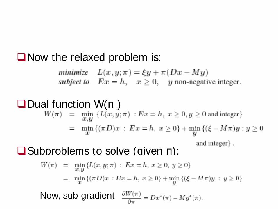
Now the relaxed problem is:

Dual function W(π )

Subproblems to solve (given π):

Now, sub-gradient

Iterative process (5.4.4b)

where update “step-size” by (5.4.4c)

Outline



Stochastic heuristics

Local Search Simulated Annealing Evolutionary Algorithms Simulated Allocation Tabu Search Others: greedy randomized

adaptive search

Local Search: steepest descent

minimize f(x) starting from initial point xc=x0

iteratively minimize value f(xc) of current state xc, by replacing it by point in its neighborhood that has lowest value.

stop if improvement no longer possible

“hill climbing” when maximizing

Problem with Local Search

may get stuck in local minima

starting point

descend direction

local minimum

global minimum

barrier to local search

Question: How to avoid local minima?

What about Occasional Ascents?

Help escaping the local optima.

desired effect

Might pass global optima after reaching it

adverse effect (easy to avoid by keeping track of best-ever state)

Simulated annealing (SAN): basic idea

From current state, pick a random successor state;

If it has better value than current state, then “accept the transition,” that is, use successor state as current state;

Otherwise, do not give up, but instead flip a coin and accept the transition with a given probability (that is lower as the successor is worse).

So we accept to sometimes “un-optimize” the value function a little with a non-zero probability.

Simulated Annealing Kirkpatrick et al. 1983:

Simulated annealing is a general method for making likely the escape from local minima by allowing jumps to higher value states.

The analogy here is with the process of annealing used by a craftsman in forging a sword from an alloy.

Real annealing: Sword

He heats the metal, then slowly cools it as he hammers the blade into shape. if he cools the blade too

quickly the metal will form patches of different composition;

if the metal is cooled slowly while it is shaped, the constituent metals will form a uniform alloy.

Simulated Annealing - algorithm

begin choose an initial solution i∈ S; select an initial temperature T > 0; while stopping criterion not true count := 0; while count < L choose randomly a neighbour j∈Ν(i); ∆F:= F(j) - F(i); if ∆F ≤ 0 then i := j else if random(0,1) < exp (-∆F / T) then i := j; count := count + 1 end while; reduce temperature (T:= T×α) end while end

Metropolis test

uphill moves are permitted but only with a certain (decreasing) probability (“temperature” dependent) according to the so called Metropolis Test

Simulated Annealing - limit theorem

limit theorem: global optimum will be found for fixed T, after sufficiently number of steps: Prob { X = i } = exp(-F(i)/T) / Z(T) Z(T) = Σj∈S exp(-F(j)/T)

for T→0, Prob { X = i } remains greater than 0 only for optimal configurations i∈S

this is not a very practical result: too many moves (number of states squared) would have to be made to achieve the limit sufficiently closely

Evolution Algorithm: motivation

A population of individuals exists in an environment with limited resources

Competition for those resources causes selection of those fitter individuals that are better adapted to the environment

These individuals act as seeds for the generation of new individuals through recombination and mutation

The new individuals have their fitness evaluated and compete (possibly also with parents) for survival.

Over time Natural selection causes a rise in the fitness of the population

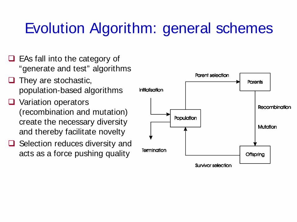
Evolution Algorithm: general schemes

EAs fall into the category of “generate and test” algorithms

They are stochastic, population-based algorithms

Variation operators (recombination and mutation) create the necessary diversity and thereby facilitate novelty

Selection reduces diversity and acts as a force pushing quality

population = a set of µ chromosomes

generation = a consecutive population

chromosome = a sequence of genes individual solution (point of the solution space) genes represent internal structure of a solution fitness function = cost function

Evolutionary Algorithm: basic notions

mutation is performed over a chromosome with certain (low)

probability it perturbs the values of the chromosome’s genes

Crossover/recombination exchanges genes between two parent chromosomes

to produce an offspring in effect the offspring has genes from both parents chromosomes with better fitness function have

greater chance to become parents

Genetic operators

In general, the operators are problem-dependent.

(M + L) - Evolutionary Algorithm

begin n:= 0; initialize(P0); while stopping criterion not true On:= ∅; for i:= 1 to L do On:= On∪crossover(Pn): for ε ∈On do mutate(ε); n:= n+1, Pn:= select_best(On∪Pn); end while end

Chromosome: x = (x1,x2,...,xD) Gene: xd = (xd1,xd2,...,xdPd) - flow pattern for the demand d 5 2 3 3 1 4 1 2 0 0 3 5 1 0 2 1 chromosome 2 3

Evolutionary Algorithm for the flow problem

Evolutionary Algorithm for the flow problem cntd.

crossover of two chromosomes each gene of the offspring is taken from one of the parents

• for each d=1,2,…,D: xd := xd(1) with probability 0.5 xd := xd(2) with probability 0.5

better fitted chromosomes have greater chance to become parents

mutation of a chromosome for each gene shift some flow from one path to another everything at random

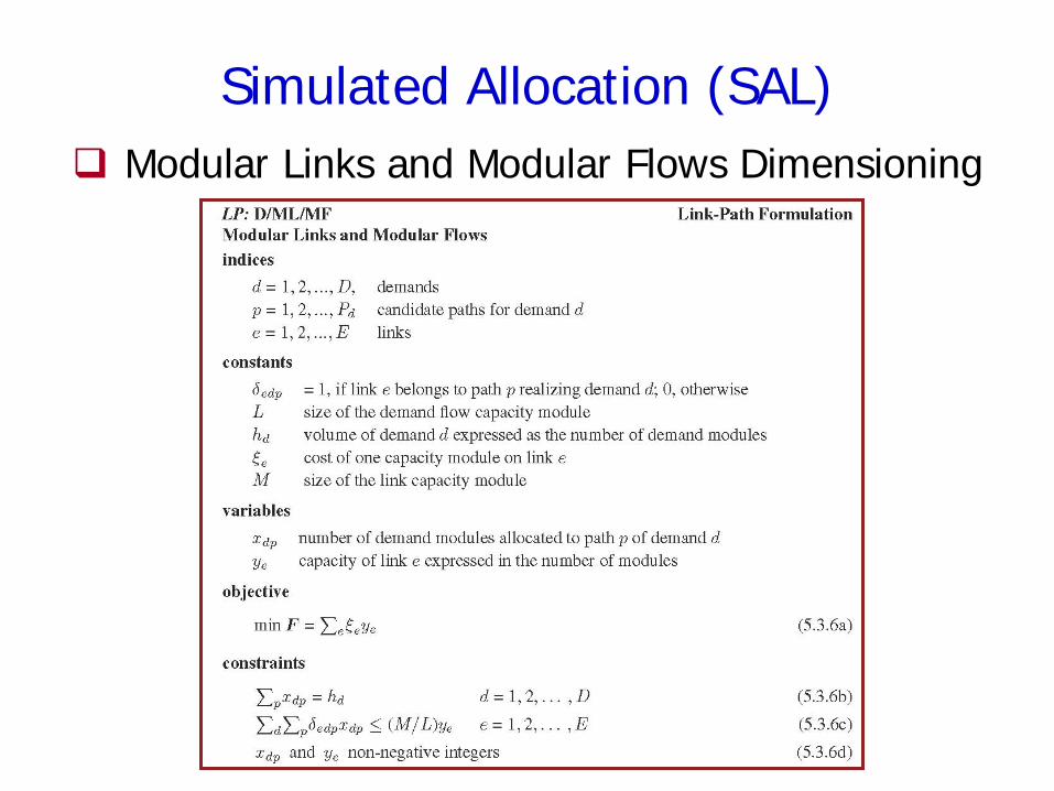
Simulated Allocation (SAL) Modular Links and Modular Flows Dimensioning

SAL: general schemes

Work with partial flow allocations some solutions NOT implement all demands

In each step chooses, with probability q(x), between: allocate(x) – adding one demand flow to the current

state x disconnect(x) – removing one or more demand flows

from current x Choose best out of N full solutions

SAL: algorithm

SAL: details

allocate(x) randomly pick one non-allocated demand module allocate demand to the shortest path

• link weight 0 if unsaturated • link weight set to the link price if saturated

increase link capacity by 1 on saturated links disconnect(x) randomly pick one allocated demand module disconnect it from the path it uses decrease link capacity by 1 for links with empty link

modules

Outline



Optimization packages

Matlab optimization toolbox

CPLEX: can solve large scale LP/IP/MIP; AMPL: a standard programming interface for

many optimization engines. Student version windows/unix/linux

• 300 variables

Matlab & optimization toolbox

Matlab: a powerful technical computing software Script-like language Rich toolboxes: optimization, statistics, symbolic

math, simulink, image processing, etc User-friendly online document/help

Optimization toolbox linprog: solve linear programming problems bintprog: solve binary integer programming problems …

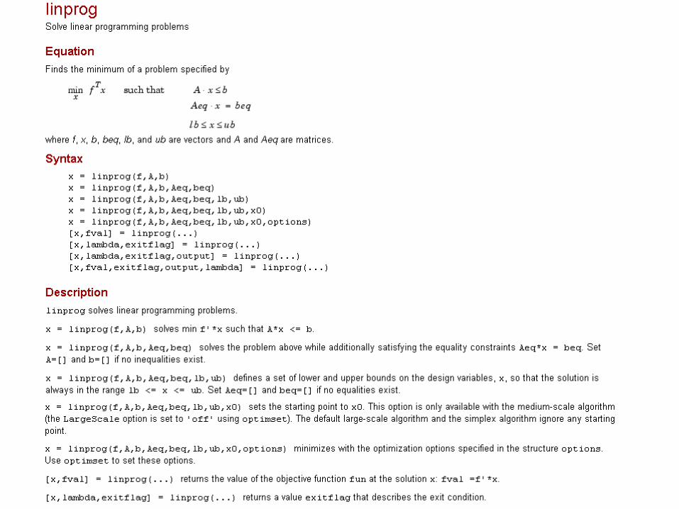
Example: linprog

Summary



Assignment

Exercise #2 Exercises 5.2 and 5.4

Additional slides: CPLEX/AMPL

Solving LP/IP/MIP with CPLEX-AMPL

CPLEX is the best LP/IP/MIP optimization engine out there.

AMPL is a standard programming interface for many optimization engines.

Student version windows/unix/linux 300 variables

Maximal Software has a free student version (up to 300 variables): uses CPLEX engine Maximal’s format is slightly different than CPLEX

format

Essential Modeling Language Features

Sets and indexing Simple sets Compound sets Computed sets

Objectives and constraints Linear, piecewise-linear Nonlinear Integer, network

. . . and many more features Express problems the various way that people do Support varied solvers

CPLEX example

Consider the following load balancing example

Will need to convert to an LP first!

In CPLEX notation, type the follow in save in file load-balance.lp

At CPLEX prompt,

Cube Network - formulation

See Appendix-D (formulation is too big to fit into a slide!)

Introduction to AMPL

Each optimization program has 2-3 files optprog.mod: the model file

• Defines a class of problems (variables, costs, constraints)

optprog.dat: the data file • Defines an instance of the class of problems

optprog.run: optional script file • Defines what variables should be saved/displayed, passes

options to the solver and issues the solve command

Running AMPL-CPLEX

Start AMPL by typing ampl at the prompt Load the model file ampl: model optprog.mod; (note semi-colon)

Load the data file ampl: data optprog.dat;

Issue solve and display commands ampl: solve; ampl: display variable_of_interest;

OR, run the run file with all of the above in it ampl: quit; prompt:~> ampl example.run

AMPL Example

minimizing maximal link utilization

AMPL: the model (I)

parameters

links

demands

routes

incidences

flow variables

AMPL: the model (II)

Objective

Constraints

AMPL: the data

optimization methods for ndp - wayne state universityhzhang/courses/7290b/lectures/05... ·...

Documents