optimization and the price of anarchy in a dynamic newsboy ... · optimization and the price of...

Optimization and the Price of Anarchy

in a Dynamic Newsboy Model

In-Koo Cho∗ Sean P. Meyn†

November 2, 2005

Abstract

This paper examines a dynamic version of the newsboy problem in which a decision makermust maintain service capacity from several sources to attempt to meet uncertain demandfor a perishable good, subject to the cost of providing sufficient capacity, and penalties fornot meeting demand.

A complete characterization of the optimal outcome is obtained when normalized demandis modeled as Brownian motion. The centralized optimal solution is a function of variabilityin demand, production variables, and the cost of insufficient capacity.

A closed form expression is obtained for the unique (state dependent) market clearingprices that allows the decentralized market to sustain the centralized optimal solution. Theprices are a non-smooth function of normalized demand and reserves. Consequently, pricesshow extreme volatility in the efficient decentralized market outcome.

Standard policy designs are examined to improve the behavior of the decentralized mar-ket, including price caps and partial decentralization where the buyer owns a portion of thetotal service capacity. It is shown that these remedies fail: The market outcome in a partiallydecentralized model is shown to be inefficient even if the buyer owns a substantial portionof the service capacity. Under the presence of a price cap, a market equilibrium, efficient ornot, fails to exist under very general conditions.

Keywords: inventory theory; newsboy model; pricing; service allocation; reliability; effi-ciency; optimization; networks.

∗I-K.C. is with the Department of Economics, University of Illinois, 1206 S. 6th Street, Champaign, IL 61820USA. [email protected], http://www.business.uiuc.edu/inkoocho

†Coordinated Science Laboratory and Department of Electrical and Computer Engineering, Uni-versity of Illinois, 1308 W. Main Street, Urbana, IL 61801 USA. [email protected],

http://www.black.csl.uiuc.edu/~meyn.

1

Optimization and the Price of Anarchy in a Dynamic Newsboy Model 2

1 Introduction

Any industry that produces perishable goods over time is faced with some version of the dynamicnewsboy’s problem. The decision maker must maintain service capacity to attempt to meetuncertain demand subject to two conflicting sources of cost: the real cost of providing sufficientcapacity, and penalties for not meeting demand. The decision maker would like to balance thesecosts in order to maximize profits subject to uncertainty and time-constraints on the rate ofproduction.

Workforce management. In a large organization such as a hospital or a call center one mustmaintain a large workforce to ensure effective delivery of services (see [40] for a recent academictreatment, or IBM’s website [3].) To increase capacity of service one must bring new employeesto work. Proper talent is usually identified and trained to be placed in position, which takestime. Alternatively, the organization can hire an employee through a temporary service agencywhich can offer talent at short notice, but at a higher price than the “usual” hiring process. Inan example such as a hospital where the cost of not meeting demand has high social cost, it iscrucial to secure a reliable channel of workers through these means, and through on-call staff.

In a complex organization these decision processes can be correspondingly complex. More-over there can be high variability in demand, and in the quality and availability of workers.This is especially true in today’s workplace since individual workers are more likely to quit thecompany.

Fashion manufacture and retail. In supplying a seasonal fashion product, the retailer maintainsa small inventory which is available at short notice, while maintaining a contract with the supplierfor deliverables in case of an unexpected surge in demand. It is more economical to have sucha contract than to maintain inventory, but it takes some time to deliver the product from theproducer to the retailer if demand increases unexpectedly [21]. In some markets demand can behighly inflexible due to “herding behavior” [6, 12, 72].

Note that this paper treats what might be a small part of a larger supply chain in the caseof manufacturing. In this case the ‘buyer’ engages the ‘seller’ to secure capacity for goods thatwill be sold to end customers.

Electric power. The electric industry is probably the largest, and arguably best known, exampleof a dynamic newsboy problem. The system operator is continuously facing the challenge ofmeeting rapidly changing demand through an array of generators that can ramp up ratherslowly due to constraints on generation as well as the complex dynamics of the power grid[36, 23]. The electricity cannot be stored economically in large quantities, yet the cost of notmeeting demand is astronomical. The massive black-out seen in the Northeast on August 14,2003, which cost $4-6 billion dollars according to the US Department of Energy, reveals thetremendous cost of service disruption [39].

In broad terms, we can state the two main objectives of investigation as follows.

1. Portfolio Management. It is a common practice in many industries to obtain multiplesources for service. The products may be very similar, but the sources of service are distinguishedby their rate of response. The central problem is to maintain an appropriate balance betweenthe various sources of reserve.


In the single-period newsboy problem the determination of the optimal service capacity basedon forecast demand can be computed through a static calculus exercise. The resulting thresholdis dependent upon cost, penalties, and the distribution of demand (see e.g. the early work ofH. Scarf [66].) Reserves have an additional benefit in a dynamic model. Positive reserves todaymake it easier to respond to a surge in demand in the future if service capacity can increase onlyslowly when compared with demand.

2. Decentralization. Decision-making is decentralized in any of the applications envisionedin this paper. It is important to understand whether the optimal solution (or some sociallydesirable solution) can be sustained by the decentralized market in which the buyers and sellersmake decisions in a decentralized manner conditioned on the market clearing price. Our centralquestion is “Can a decentralized market internalize through a market clearing price the variousbenefits furnished by available service capacity?”

1.1 Summary of models and conclusions

We examine an idealized model in which a firm produces and delivers a good to the consumer incontinuous time. The good is perishable, in that it must be consumed immediately. This is thecase in electric power or temporary services, and to a lessor extent fashionable clothing. Thefirm has access to a number of sources of service that can produce the good.

The social value is realized as the good is delivered and consumed. On the other hand, ifsome demand is not met, the social cost is proportional to the size of the excess demand. Itis assumed that the mean demand is met by primary service (the cheapest source of servicecapacity) through a long term contract.

On-going demand can be met through primary service, as well as K ≥ 1 sources of ancillaryservice.

Other constraints and costs assumed in the model are,

• Constrained production and free disposal: Service capacity at time t from primaryand ancillary services are denoted {Gp(t), Ga1(t), . . . , GaK (t)}. Capacity is rate constrained:Gp(t) can increase at maximal rate ζp+, and Gak(t) can increase at maximal rate ζak+ < ∞.Increasing capacity takes time, but the decision maker can freely (and instantaneously) disposeof excess capacity if he chooses to do so.

• Constant marginal capacity cost: cp is the cost per unit capacity for primary service,and cak the cost of building one additional unit of capacity from the kth source of ancillaryservice. The cost parameters are ordered, cp < ca1 < · · · < caK .

• Constant marginal dis-utility of shortage: Let Ga(t) :=∑

i Gai(t), and

Q(t) = Gp(t) + Ga(t) − D(t), t ≥ 0 . (1.1)

be the excess capacity at time t. The marginal cost of excess demand is denoted cbo > 0, sothat the social cost of excess demand is given by cbo max(−Q(t), 0). The larger the shortage,the greater the damage to society. It is assumed that

cbo > caK > · · · > ca1 > cp.


When normalized demand is modeled as a driftless Brownian motion the system is viewed asa (K + 1)-dimensional constrained diffusion model. A complete characterization of the optimalportfolio of service capacities is computed, thereby resolving the first issue presented above. Theoptimal policy is constructed explicitly through a detailed analysis of the dynamic programmingequations for the multidimensional model, and is found to be of the precise affine form introducedin [18]. The optimal solution clearly reveals how volatility of demand and the productiontechnology of service influences the size, the composition, and the dynamics of optimal servicecapacity.

Our assumptions do lead to an idealized model. In particular, in a real electric power systemthe cost of generation is non-linear and even non-convex. As we suppress non-convexity of theproduction cost we eliminate one source that is known to prevent the decentralized market fromsustaining the centralized optimal solution. Consequently, this idealization makes the analysistractable, but also strengthens the key policy implications of this paper. The decentralizedspot market will not function as envisioned by policy makers whose intention is to protect theinterests of the consumers. That is, even if the spot market can sustain the optimal solution,the payoff to the consumers in the efficient outcome is precisely what they would obtain if theychose to purchase no reserve, resulting in frequent black-outs. In fact, the generator extractsthe entire gains from trading in the efficient market outcome.

These conclusions are based upon a calculation of the unique equilibrium price functionalthat can possibly sustain the optimal centralized solution as the market outcome. The priceat time t is expressed as a piecewise smooth function of the excess capacity Q(t) = q and thedemand D(t) = d,

pp(q, d) = pak(q, d) = (cbo + v)max(d, 0) − max(−q, 0)

d + qk = 1, . . . ,K (1.2)

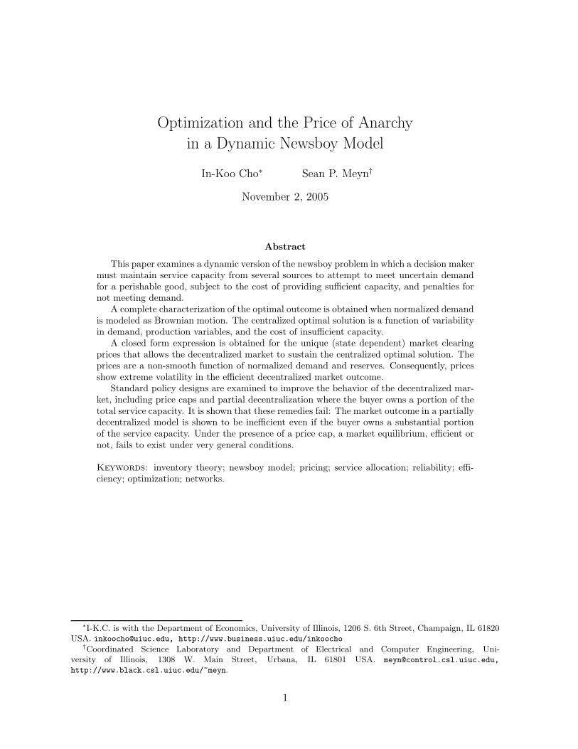
where cbo is the marginal cost of not meeting demand, and v is the marginal value of the product.The plot shown in Figure 1 shows a simulation of prices, demand D, and reserves Q based

on the Markovian price functional (1.2) for the “controlled random-walk” model introduced inSection 2.3.

The price functional is simple and intuitive. Because the buyer does not differentiate whichservice produced the good, the market prices of primary and ancillary services coincide. Theprice reaches its maximum value cbo + v whenever Q(t) < 0 and D(t) > 0, and is zero whenthese inequalities are reversed. Volatility of the price as a function of time will sometimes begreater than the volatility in demand.

The conclusions obtained for the idealized model considered here demonstrate that volatilityand high prices can be expected in a deregulated market whenever the market achieves anefficient allocation, even without market manipulation.

These conclusions offer new insight to the events in California following deregulation ofthe ancillary service market. Brien in [15] gives a summary of the ancillary services marketin California as it existed in 1999, and lists several benefits of ancillary services, includingstabilization of voltage and frequency, and the option to extract or dump energy at short notice.She notes that on July 12, 1998, prices for one source of reserve reached $9,999/MWh for severalhours, more than one-hundred times the marginal cost (see also [15, 74, 63].) It appears thathigh prices were due in part to deliberate manipulation, but high prices and volatility have beenobserved in other electric power markets. Extreme volatility and unprecedented high prices forpower were seen in the partially deregulated market in Illinois in the summer of 1998. High


100

150

0

50

200

250

Mon Tue Wed Thu Fri Sat Sun

Prices

Normalized demand

Reserve

Figure 1: Prices as a function of demand and reserves in the efficient equilibrium, based on the Markovian pricefunctional (1.2).

100

150

0

50

200

250

300

Mon Tue Wed Thu Fri Sat Sun

Prices (Eur/MWh)

Marginal cost (est.)

Week 25

Week 26

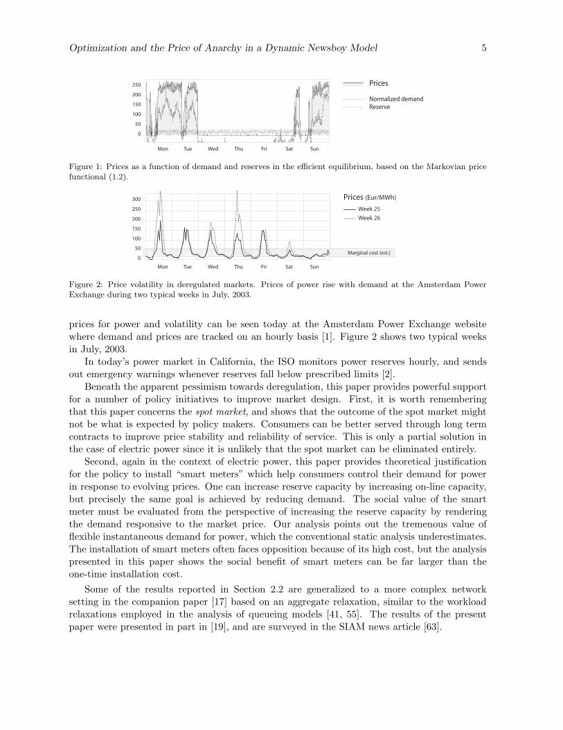
Figure 2: Price volatility in deregulated markets. Prices of power rise with demand at the Amsterdam PowerExchange during two typical weeks in July, 2003.

prices for power and volatility can be seen today at the Amsterdam Power Exchange websitewhere demand and prices are tracked on an hourly basis [1]. Figure 2 shows two typical weeksin July, 2003.

In today’s power market in California, the ISO monitors power reserves hourly, and sendsout emergency warnings whenever reserves fall below prescribed limits [2].

Beneath the apparent pessimism towards deregulation, this paper provides powerful supportfor a number of policy initiatives to improve market design. First, it is worth rememberingthat this paper concerns the spot market, and shows that the outcome of the spot market mightnot be what is expected by policy makers. Consumers can be better served through long termcontracts to improve price stability and reliability of service. This is only a partial solution inthe case of electric power since it is unlikely that the spot market can be eliminated entirely.

Second, again in the context of electric power, this paper provides theoretical justificationfor the policy to install “smart meters” which help consumers control their demand for powerin response to evolving prices. One can increase reserve capacity by increasing on-line capacity,but precisely the same goal is achieved by reducing demand. The social value of the smartmeter must be evaluated from the perspective of increasing the reserve capacity by renderingthe demand responsive to the market price. Our analysis points out the tremenous value offlexible instantaneous demand for power, which the conventional static analysis underestimates.The installation of smart meters often faces opposition because of its high cost, but the analysispresented in this paper shows the social benefit of smart meters can be far larger than theone-time installation cost.

Some of the results reported in Section 2.2 are generalized to a more complex networksetting in the companion paper [17] based on an aggregate relaxation, similar to the workloadrelaxations employed in the analysis of queueing models [41, 55]. The results of the presentpaper were presented in part in [19], and are surveyed in the SIAM news article [63].


1.2 Background

At the close of the 1950s, Herbert Scarf obtained the optimal policy for a single period newsboyproblem and showed that it is of a threshold form [66, 67], following previous research oninventory models by Arrow et. al. [4] and by Bellman ([10] and [9, Chapter 5].) Scarf points outin [66] that the conclusion that the solution is defined by a threshold follows from the convexityof the value function with respect to the decision variables. These structural issues are alsodeveloped in [9], and in dozens of papers published over the past fifty years.

Following these results there was an intense research program concerning the control of one-dimensional inventory models, e.g. [35, 75, 64, 69, 7, 24, 58]. More recently there have been effortsin various directions to develop hedging (or safety stocks) in multidimensional inventory modelsto improve the performance of the system [33, 28, 29, 68] (especially in terms of responsiveness[31]), or obtain approximate optimality [41, 46, 32, 8, 55, 51, 52, 18, 70].

The results on centralized optimal control obtained here are most closely related to resultsreported in [18, 56]. It is shown that for a large class of multiclass, multidimensional networkmodels, an optimal policy can be approximated in “workload space” by a generalized thresholdpolicy. It is called an affine policy since it is constructed as an affine translation of the optimalpolicy for a fluid model. In particular, [18, Theorem 4.4] establishes affine approximations underthe discounted cost criterion, and [18, Proposition 4.5 and Theorem 4.7] establishes similarresults under the average cost criterion for a diffusion model. The method of proof reduces theoptimization problem to a static optimization calculation based on a one-dimensional reflectedBrownian motion (see also the discussion surrounding the height process (A.7) below.) Ananalogous calculation is performed in [71] in the analysis of a one-dimensional inventory model.Consequently, the formula for the optimal affine parameter obtained in [18, Proposition 4.5 andTheorem 4.7] coincides with the formula presented in [71, Proposition 3], and is similar to thethreshold values given in (2.17).

The newsboy’s problem has been investigated from the perspective of a central decisionmaker who can control the size of inventory dynamically. The decentralized dynamic newsboy’sproblem has received much less attention. The bulk of research has concentrated on joint pricingand inventory control in a single-period model, based on a functional model of demand vs. price- see surveys in [47, 62, 11]. Dynamic versions of this problem are treated in recent work (see[61, 43, 59, 11] and the references therein.) In some special cases it is found that price is roughlyindependent of state [61], but this conclusion cannot be expected to hold in general [43, 11].

Recently Van Mieghem has provided a complete analysis of a two-period newsboy modelwith two sources of service [57]. The framework is different, but some conclusions are similar tothose obtained here. In particular, under certain conditions a unique Markovian price functionalis obtained that can support the centralized optimal outcome.

The “price of anarchy” in the title refers to recent work of Papadimitriou, Tardos, Tsitsiklis,and Johari concerning Nash equilibria in static networks intended to model Internet routing[44, 65, 38, 37], and Johari also considers power networks in the thesis [37]. These results extendBraess’s celebrated “paradox” on efficiency of networks by demonstrating that the worst-casecost of a Nash flow is at most 33% above the optimal solution. These recent results concerngeneral networks, and even contain extensions to nonlinear cost on links. However, one purposeof this paper is to send out a warning: The cost of deregulation may be enormous for some ofthe players in even a very simple dynamic network.

The remainder of the paper is organized as follows. Section 2 describes the diffusion model


in which normalized demand is a Brownian motion. The main results of this paper are collectedin Sections 2.2 and 2.4. The development of optimal centralized control is contained in thefirst half of Section 3. The decentralized problem is the focus of Sections 3.4 and 3.5, wherethe Gaussian assumption on demand is relaxed, and the price functional (1.2) is constructed.Proofs of the major results are contained in the Appendix. Section 4 concludes the paper.

2 Dynamic Newsboy Model and Main Results

This section summarizes the main results of this paper. A diffusion model is considered inthe simplest case in which there is a single customer (referred to as a buyer) that is served byprimary and ancillary services. For the moment it is assumed that the buyer can access only asingle source of ancillary service. It is assumed that the two sources of service are owned by thesame firm, simply called the supplier (or the seller).

The analysis is extended to multiple sources of service in Section 3.3.

2.1 Diffusion Model

Recall that service capacity at time t from the primary and ancillary services are denoted{Gp(t), Ga(t)}. Demand is denoted D(t), and reserve at time t is defined by Q(t) = Gp(t) +Ga(t) − D(t) as expressed in (1.1). The event Q(t) < 0 is interpreted as the failure of reliableservices. In the application to electric power this represents black-out since the demand forpower exceeds supply.

We impose the constraint that Ga(t) ≥ 0 for all t, but Gp(t) is not sign-constrained.We sometimes refer to Gp(t)+Ga(t) as the on-line capacity, since the seller can offer primary

and ancillary services Gp(t) and Ga(t) instantaneously at time t. Capacity is subject to rampingconstraints: For finite, positive constants ζp+, ζa+,

Gp(t′) − Gp(t)

t′ − t≤ ζp+ and

Ga(t′) − Ga(t)

t′ − t≤ ζa+ for all t′ > t ≥ 0.

We assume the free disposal of the capacity, which implies that Gp(t) and Ga(t) can decreaseinfinitely quickly. The ramping constraints can be equivalently expressed through the equations,

Gp(t) = Gp(0) − Ip(t) + ζp+t , Ga(t) = Ga(0) − Ia(t) + ζa+t , t ≥ 0, (2.1)

where the idleness processes {Ip, Ia} are non-decreasing. It is assumed that D(0) is given as aninitial condition, and primary service is initialized using the definition (1.1),

Gp(0) = Q(0) + D(0) − Ga(0).

Throughout most of the paper it is assumed that D(0) = 0. Essentially, we assume that thebuyer has a long term contract with the seller of primary service to take care of the mean demand.In the context of the electricity market, the supplier is the power generator, and the buyer is a“representative” consumer, who takes care of the “expected” demand for power through a longterm contract, but wants to procure additional capacity to ensure reliability of service. Underthis interpretation, the “outside” option for the buyer is not to purchase any reserve capacity.Our focus is how to maximize “social surplus” by balancing the size of the capacities of servicesin response to uncertain demand.


Until Section 3.4 it is assumed that D is a driftless Brownian motion, with instantaneousvariance denoted σ2

D > 0. The model (1.1) is then called the controlled Brownian motion (CBM)model, with two-dimensional state process X :=(Q,Ga)T. A Gaussian model for demand mightbe justified by considering a Central Limit Theorem scaling of a large number of individualdemand processes, as in [42]. Rather than attempt to justify a limiting model, here we choosea Gaussian demand model for the purposes of control design.

Under this assumption, the state process X evolves according to the Ito equation,

dX = δX − BdI(t) − dD(t), t ≥ 0 , (2.2)

where δX = (ζp+ + ζa+, ζa+)T, X(0) = (q, ga)T ∈ X = R × R+ is given as an initial condition,and the 2 × 2 matrix B is defined by,

B =

[1 10 1

]. (2.3)

It is assumed that that the process I = (Ip, Ia)T appearing in (2.1) and (2.2) is adapted to D,and that the resulting state process X is constrained to the state space X = R×R+. A processI satisfying these constraints is called admissible.

In what follows we restrict to stationary Markov policies defined as a family of admissibleidleness processes {Ix}, parameterized by the initial condition x ∈ X, with the defining propertythat the controlled process X is a strong Markov process on X.

For x ∈ R we denote,

x+ = max(x, 0), x− = max(−x, 0) = (−x)+.

An affine policy for the CBM model (2.2) is based on a pair of thresholds (qp, qa):

(i) For a given initial condition X(0) = x = (q, ga)T ∈ X,

X(0+) =

(qga

)− µ

(11

), ga ≥ q − qp

(qp

0

), ga ≤ q − qp.

(2.4)

where µ:=min((q− qa)+, ga) ≥ 0. The potential jump at time t = 0 reflects the assumptionthat the seller can freely reduce capacity instantaneously.

Consequently, for t > 0 the state process X is restricted to the smaller state space givenby R(q) := closure (Rp ∪Ra), where

Ra = {x ∈ X : x1 < qa, x2 ≥ 0}, Rp = Ra ∪ {x ∈ X : x1 < qp, x2 = 0}. (2.5)

(ii) For any t > 0, if Q(t) < qp, then ddt

Gp(t) = ζp+, and if Q(t) < qa then ddt

Ga(t) = ζa+.Consequently, the following boundary constraints hold with probability one,

∫ ∞

0I{X(t) ∈ Rp} dIp(t) =

∫ ∞

0I{X(t) ∈ Ra} dIa(t) = 0. (2.6)

A sketch of a typical sample path of X under an affine policy is shown in Figure 3. From theinitial condition shown, the process has mean drift δX up until the first time that Q(t) reachesthe threshold qa. The subsequent downward motion shown is a consequence of reflection at theboundary of Ra. Since Q(t) remains near qa yet primary service is ramped up at maximumrate ζp+, it follows that ancillary service has long-run average drift of −ζp+ up until the firsttime that Ga(t) reaches zero. For the fluid model in which σ2

D = 0 we have ddt

Ga(t) = ζa+ when

Q(t) < qa, ddt

Ga(t) = −ζp+ whenever Ga(t) > 0 and Q(t) = qa.


0 q a q p

Q

X(t)

Ga

Figure 3: Trajectory of the two-dimensional model under an affine policy

2.2 Optimization

Recall that cp, ca denote the cost for maintaining one additional unit of capacity for primaryand ancillary services. It is assumed that the marginal cost of production is higher for ancillaryservice,

cp < ca.

Welfare functions for the supplier and consumer are defined respectively by,

WS(t) := (pp − cp)Gp(t) + (pa − ca)Ga(t)

WD(t) := v min(D(t), Gp(t) + Ga(t)) −(ppGp(t) + paGa(t) + cboQ−(t)

).

(2.7)

The supplier is paid for the “on-line” capacity rather than the services delivered. For ex-ample, in an application to power the generator may have to burn coal in order to maintain acertain level of on-line capacity. On the other hand, the consumer obtains surplus only from thepower delivered.

The welfare function for the consumer can be simplified,

WD(t) = vD(t) −(ppGp(t) + paGa(t) + (cbo + v)Q−(t)

), (2.8)

where we have used the identity,

min(D(t), Gp(t) + Ga(t)) = min(D(t), Q(t) + D(t)) = D(t) − Q−(t).

In the centralized problem the network is controlled by an impartial agent, called the socialplanner, who is given full authority over the buyer and the seller to achieve the best possibleoutcome. The social surplus at time t is given by,

W(t) = WS(t) + WD(t)

We have Gp(t) = Q(t) + D(t) − Ga(t), so that the social surplus is equivalently expressed,

W(t) = vD(t) − [cpGp(t) + caGa(t) + (cbo + v)Q−(t)]

= (v − cp)D(t) − [cpQ(t) + (ca − cp)Ga(t) + (cbo + v)Q−(t)]

= (v − cp)D(t) − C(t),

whereC(t) := c(X(t)) := cpQ(t) + (ca − cp)Ga(t) + (cbo + v)Q−(t). (2.9)


For a given initial condition D(0) = d for demand we have d = E[D(t)], and hence,

E[W(t)] = (v − cp)d − E[C(t)], t ≥ 0. (2.10)

Motivated by the representation (2.10), we consider each of the two cost-criteria,

Average cost: φ := lim supT→∞

Ex

[ 1

T

∫ T

0c(X(t)) dt

](2.11)

Discounted cost: K(x) := Ex

[∫ ∞

0e−ηtc(X(t)) dt

], (2.12)

where η > 0 is the discount parameter, and x ∈ X is the initial condition of X. Our goal is tominimize the given criterion over all stationary policies.

Before pursuing optimization, let us first consider some simple sub-optimal policies.One approach is ‘open-loop’: The buyer can trust the ‘long term contract’ already secured

to meet mean-demand, and then choose Gp = Ga ≡ 0. Based on (2.7) this leads to WS(t) = 0and

WD(t) = −(vD−(t) + cboD+(t)

). (2.13)

If D(0) = 0 this then gives,

E[WD(t)] = −12(cbo + v)E[|D(t)|] = −1

2(cbo + v)σD

√t. (2.14)

This is precisely the payoff of the consumer at t if no reserve capacity is procured: Ga(t) =Gp(t) = 0. We consider this value as the “outside” option for the buyer in the market. Thus, inorder to check the individual rationality of a market outcome, we use this value as the benchmark.Note that regardless of the initial condition we see that the mean welfare for the buyer and thesocial surplus simultaneously diverge to −∞ as t → ∞.

Consider next an arbitrary affine policy. The steady-state social surplus can be computedbased on the following result of [17].

Theorem 2.1 For any affine policy, the Markov process X is exponentially ergodic [25]. Theunique stationary distribution π on X satisfies,

(i) The first marginal of π is given by the distribution function,

Pπ{Q(t) ≤ q} =

{e−γp(qp−q) qa ≤ q ≤ qp

e−γp(qp−qa)−γa(qa−q) q ≤ qa,

where

γa = 2ζp+ + ζa+

σ2D

, γp = 2ζp+

σ2D

. (2.15)

(ii) The steady state mean of the cost c : X → R+ defined in (2.9) is explicitly computable,

φ(q) := π(c) = γ−1a

(ζa+

ζp+ca + e−γaqa

(cbo + v))e−γp(qp−qa) + (qp − γ−1

p )cp. (2.16)

⊓⊔


Consequently, the steady-state mean welfare functions of the seller and buyer are computablewhen prices are fixed:

Corollary 2.2 For any affine policy the steady-state mean social surplus is given by

limt→∞

E[W(t)] = −φ(q),

where φ is given in (2.16), and the convergence is exponentially fast. Moreover, if the prices(pp, pa) are fixed, then the individual welfare functions have finite steady-state means,

limt→∞

E[WS(t)] = γ−1a

ζa+

ζp+(pa − ca)e−γp(qp−qa) + (qp − γ−1

p )(pp − cp)

limt→∞

E[WD(t)] = −[γ−1

a

(ζa+

ζp+pa + e−γa qa

(cbo + v))e−γp(qp−qa) + (qp − γ−1

p )pp

].

When D(t) has zero-mean and the prices are fixed with pp ≤ pa ≤ cbo + v then necessarilyE[WD(t)] < 0: Exactly as in the derivation of (2.10) we have,

E[WD(t)] = −E[ppQ(t) + (pa − pp)Ga(t) + (cbo + v)Q−(t)], t ≥ 0.

This is the inevitable ‘cost of variability’, i.e. risk, as seen by the buyer. Since we have assumedthat demand is normalized, the buyer sees additional value arising from the contract purchaseof mean-demand at time 0−.

In conclusion, although the residual mean welfare seen by the buyer is always negative, thereremains much benefit to engage the seller for services if the prices are not too high. As clearlyshown in (2.13), the alternative ‘open-loop’ strategy is not sustainable.

q p− qa

qa q p− qa

qa

12

34

56

7

12

13

14

16

17

18

18

20

22

24

12

34

56

7

12

13

14

16

17

18

18

20

22

24

15 15

Figure 4: Shown at left is the average cost obtained using simulation for the network considered in Section 2.3with Bernoulli noise using various affine parameters. At right is the average cost obtained from Theorem 2.1 (ii)for the CBM model.

The following two theorems describe the optimal policy for the social planner under the twocost criteria (2.11), (2.12). The proof of Theorem 2.3 is contained in Section 3.2. It is remarkablethat the optimal policy is computable for this multi-dimensional model, and that the optimalsolution is of this simple affine form.


Theorem 2.3 The average-cost optimal policy (over all stationary policies) is affine, with spe-cific parameter values given by,

qa∗ = γ−1a ln

(cbo + v

ca

)qp∗ = qa∗ + γ−1

p ln

(ca

cp

). (2.17)

⊓⊔

From Theorem 2.1 (ii) it can be shown that the average cost is convex as a function of(qp, qa), with unique minimum given in (2.17). This is plainly illustrated in the plot shown atright in Figure 4.

The proof of Theorem 2.4 is similar to the proof of Theorem 2.3. Computation of theparameters in (2.18) is provided in [16].

Theorem 2.4 The optimal policy under the discounted-cost control criterion is affine for aunique pair of parameters given by

qp∗η =

σ2D

ζp+ + mp

(ln

ca

cp+

ζp+ + mp

ζ+ + mln

cbo + v

ca

),

qa∗η = 1

2

σ2D

ζp+ + ζa+

(ln

cbo + v

ca+ ln

ζa+

ζp++ ln

−ζa+ + mp + m

2ζa+

),

(2.18)

where

mp =√

(ζp+)2 + 2σ2Dη , m =

√(ζ+)2 + 2σ2

Dη.

Furthermore qp∗η → qp∗ and qa∗

η → qa∗ as η → 0, where qp∗ and qa∗ are given in (2.17). ⊓⊔

Theorem 2.3 and Theorem 2.4 have clear implications to the decentralized market problem:if the prices {cp, ca} are the prices charged to the buyer by the seller, the seller will assume thatthe buyer will optimize based on what it is charged. The formulae given in these two theoremsquantify the observation: When γp is small, then the fair price for ancillary service may beextremely high. The parameter γp is small if there is significant variability in demand, or if themaximum ramp-up rate for primary service is small. This is an important observation criticalfor interpreting a market outcome sustaining the optimal allocation.

Before turning to the decentralized model we present numerical results illustrating the con-clusions of Theorem 2.3.

2.3 Numerical Examples

In this section we present some numerical results based on simulation and dynamic programmingexperiments. These plots are taken from [16] where the reader can find further numerical results.

Simulation and optimization will be performed for a two-dimensional controlled random-walk(CRW) model which evolves in discrete time. The forecasted excess capacity at time t ≥ 1 isagain defined by (1.1), where D(t) is the demand at time t, and (Gp(t), Ga(t)) are currentcapacity levels from primary and ancillary service. It is assumed that D is a random walk

D(t) =t∑

s=1

E(s), t = 1, 2, . . . ,


σ2

D = 6 σ2

D = 18 σ2

D = 24

qp∗ = 9.2 qp∗ = 27.6 qp∗ = 36.8

qp≈ 9.2 qp

≈ 26 qp≈ 32

qa≈ 2.3 ≈ 8.3qa

≈ 5 qa

qa∗ = 2.3 qa∗ = 6.9 qa∗ = 9.2

CRW model

CBM model

10- 10 0 20- 20 30

10

20

30

40

ga

10- 10 0 20- 20 30

10

20

30

40

ga

q

10- 10 0 20- 20 30

10

20

30

40

ga

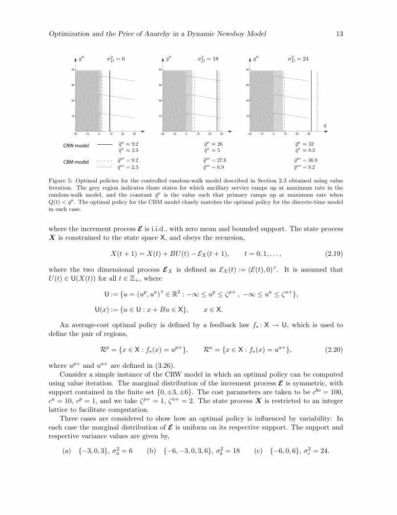
Figure 5: Optimal policies for the controlled random-walk model described in Section 2.3 obtained using valueiteration. The grey region indicates those states for which ancillary service ramps up at maximum rate in therandom-walk model, and the constant qp is the value such that primary ramps up at maximum rate whenQ(t) < qp. The optimal policy for the CBM model closely matches the optimal policy for the discrete-time modelin each case.

where the increment process E is i.i.d., with zero mean and bounded support. The state processX is constrained to the state space X, and obeys the recursion,

X(t + 1) = X(t) + BU(t) − EX(t + 1), t = 0, 1, . . . , (2.19)

where the two dimensional process EX is defined as EX(t) := (E(t), 0)T. It is assumed thatU(t) ∈ U(X(t)) for all t ∈ Z+, where

U := {u = (up, ua)T ∈ R2 : −∞ ≤ up ≤ ζp+ , −∞ ≤ ua ≤ ζa+},

U(x) := {u ∈ U : x + Bu ∈ X}, x ∈ X.

An average-cost optimal policy is defined by a feedback law f∗ : X → U, which is used todefine the pair of regions,

Rp = {x ∈ X : f∗(x) = up+}, Ra = {x ∈ X : f∗(x) = ua+}, (2.20)

where up+ and ua+ are defined in (3.26).Consider a simple instance of the CRW model in which an optimal policy can be computed

using value iteration. The marginal distribution of the increment process E is symmetric, withsupport contained in the finite set {0,±3,±6}. The cost parameters are taken to be cbo = 100,ca = 10, cp = 1, and we take ζp+ = 1, ζa+ = 2. The state process X is restricted to an integerlattice to facilitate computation.

Three cases are considered to show how an optimal policy is influenced by variability: Ineach case the marginal distribution of E is uniform on its respective support. The support andrespective variance values are given by,

(a) {−3, 0, 3}, σ2a = 6 (b) {−6,−3, 0, 3, 6}, σ2

b = 18 (c) {−6, 0, 6}, σ2c = 24.


The marginal distribution has zero mean since the support is symmetric in each case.The average-cost optimal policy was computed for the three different models using value

iteration. Results from these experiments are illustrated in Figure 5: The constant qp is definedas the maximum of q ≥ 0 such that Up(t) = 1 when X(t) = (q, 0)T. The grey region representsRa, and the constant qa is an approximation of the value of q for x on the right-hand boundaryof Ra.

Also shown in Figure 5 is a representation of the optimal policy for the CBM model withfirst and second order statistics consistent with the CRW model. That is, the demand processD was taken to be a drift-less Brownian motion with variance σ2

D equal to 6, 18, or 24 as shownin the figure. The constants qp∗, qa∗ indicated in the figure are the optimal parameters for theCBM model given in (2.17). The optimal policy for the CBM model closely matches the optimalpolicy for the discrete-time model in each case.

We consider now a simulation experiment based on a family of affine policies for the CRWmodel.

The model parameters used in this simulation are as follows: v = 0, cp = 1, ca = 20,and cbo = 400. The ramp-up rates were taken as ζp+ = 1/10 and ζa+ = 2/5. The marginaldistribution of the increment distribution was taken symmetric on {±1}.

Shown at right in Figure 4 is the average cost obtained from Theorem 2.1 (ii) for the CBMmodel with first and second order statistics identical to those of the CRW model. For thesenumerical values, (2.17) gives (qp∗, qa∗) = (17.974, 2.996).

Affine policies for the CRW model were constructed based on threshold values {qp, qa}. Theaverage cost was approximated under several values of (qp, qa) based on the (unbiased) smoothedestimator of [34] (for details see [16].) In the simulation shown at left in Figure 4 the time-horizonwas n = 8 × 105. Among the affine parameters considered, the best policy for the discrete timemodel is given by (qp∗, qa∗) = (19, 3), which almost coincides with the values obtained using(2.17). The thesis [16] contains similar simulations in which E is Markov rather than i.i.d..Similar solidarity is seen in these experiments when σ2

D is taken to be the asymptotic varianceappearing in the Central Limit Theorem for E .

In conclusion, in-spite of the drastically different demand statistics, the best affine policyfor the discrete-time model is remarkably similar to the average-cost optimal policy for thecontinuous-time model with Gaussian demand. Moreover, the optimal average cost for the twomodels are in close agreement.

2.4 Dynamic equilibria

A fundamental question is whether we can implement the centralized solution through a decen-tralized market mechanism. For analytic convenience we restrict to a Markovian price mecha-nism in which the market prices at time t are completely determined by (Q(t), Ga(t), Gp(t)) fort ≥ 0. This is Markovian with respect to the three-dimensional CBM model X† := (Q,Ga,D)T.

While the market clearing price may depend upon the entire history of the market outcome ingeneral, this restriction is reasonable given the Markovian nature of the model, as we demonstratein the far more general setting of Section 3.4.

A decentralized, discounted optimal control problem is formulated as follows. Let p(x, d) ={pa(x, d), pp(x, d)} denote the pair of market clearing prices given X(t) = (Q(t), Ga(t)) = (q, ga)and D(t) = d at time t. Given the functional p : (X × R)2 → R

2, the buyer and seller solve the


respective optimization problems,

maxE

[∫e−ηtWS(t) dt

], maxE

[∫e−ηtWD(t) dt

],

where the definitions (2.7) are maintained based on p = (pa, pp).The optimization problem of the central planner and that of the consumer are very similar:

WD(t) is obtained by replacing (ca, cp) by p. However, there are two important differences thathave profound economic implications. First, in the decentralized market ramping rates are notconsidered in the optimization problem posed by the buyer. Second, while the cost parameters(ca, cp) are assumed constant, the prices can fluctuate with the evolving state process. The firstobservation greatly simplifies the optimization problem of the consumer. Unfortunately, thesecond observation prevents us from applying directly the analysis developed for the centralizedproblem.

For a given price functional p, let (Gad(p),Gp

d(p)) and (Gas(p),Gp

s(p)) denote the respectivesolutions of the optimization problems for the consumer and supplier. We then define,

(i) The pair (Ga,Gp) is called a centralized solution for a given initial state x ∈ X if it achievesthe optimal cost (discounted or average, depending upon the context.)

(ii) The triple (p,Ga,Gp) is called a decentralized market outcome if p clears the market :

Ga = Gad(p) = Ga

s(p), Gp = Gpd(p) = Gp

s(p).

If this holds for each initial condition then p is called an equilibrium price functional.

(iii) Let (Ga,Gp) be a centralized solution for a given initial state x ∈ X. A decentralizedmarket outcome sustains the centralized solution if there exists a functional p such thatthe triple (p,Ga,Gp) forms a decentralized market outcome for the same initial conditionx. We say that the second welfare theorem holds if it is possible to construct a decentralizedmarket outcome that sustains the centralized solution from each initial condition.

Two real-valued functions f, g on X are regarded as equal if f(x) = g(x) for a.e. x ∈ X withrespect to Lebesgue measure. Similarly, when an equilibrium price functional is declared to beunique, it is understood that this uniqueness holds almost everywhere.

The calculation of the price functional provides important insights about the operation ofthe decentralized market, and also allows us to calculate the expected payoff in the decentralizedmarket outcome, which reveals a serious problem in the decentralized market:

Theorem 2.5 The second welfare theorem holds. There is a unique equilibrium price functionalthat is Markovian with respect to (X,D), and it is expressed by (1.2). This price functionalsustains the centralized optimal solution as the decentralized market outcome, and the resultingoptimized objective function of the buyer results in (2.13):

WD(t) = −(vD−(t) + cboD+(t)

).

⊓⊔

Theorem 2.5 has several subtle consequences. In the following paragraphs we explore severalpolicies that are commonly proposed to improve the market. We conclude with comments onthe impact of responsive demand.

We begin with a few remarks on the unique dynamic equilibrium obtained in Theorem 2.5.


2.4.1 Fairness

While the second welfare theorem offers rationale for deregulation, the same result does not tellus whether the market outcome is “fair” in any reasonable sense.

Theorem 2.5 states that the welfare seen by the buyer is precisely what the buyer wouldattain using the open-loop policy Gp = Ga ≡ 0, as shown in (2.13). By the same token, themean surplus of the seller in period t is

E[WS(t)] ≫ E[W(t)].

In particular, in the CBM model in which demand has zero mean, the expected payoff at timet given in (2.14) is E[WD(t)] = −1

2(cbo + v)σD

√t < 0. Hence, the buyer can never generate

positive surplus by participating in the decentralized market [22, 60, 45, 73].If demand is normalized so that E[D(t)] = 0 for all t ≥ 0 then one might claim that the

negative expected payoff for the buyer is a natural consequence of this normalization. A carefulexamination shows otherwise. The theorem states that WD(t) < 0 whenever D(t) 6= 0, even ifD is initialized at some value D(0) > 0.

Recall that the buyer has no alternative way to procure reseve capacity to improve the reli-ability of service. Under this restriction, the consumer is essentially exploited by the generatorsin the efficient market, paying an enormous price for reliability.

2.4.2 Price caps

In Proposition 3.6 we show that (1.2) is the only candidate equilibrium price functional. Con-sequently,

Corollary 2.6 If a price cap p is imposed with p < v + cbo then the resulting market does notadmit any Markovian equilibrium price functional.

Note that the corollary says that there is no equilibrium of any kind, efficient (in the sensethat it sustains the centralized solution) or not. The proof follows from Proposition 3.6 and thefact that p < maxx,d p(x, d) under the assumptions of the corollary.

2.4.3 Semi-Unified ownership

The fundamental problem of the decentralized market is that the buyer must pay a very highprice in order to internalize the social benefit of sufficient service capacity. A possible remedywould to allow the buyer control service capacity, which would bring us back to the centralizedregime.

Here we examine an intermediate setting in which the buyer owns primary service, whileancillary services remain under the ownership of a separate entity. For simplicity, we considerthe case where there is a single source of ancillary service, and we restrict to the case where theprice functional is Markovian with respect to X† = (X ,D) with D Brownian motion.

If the buyer controls primary service then we can consider the decentralized problem withwelfare functions

WS(t) := (pa − ca)Ga(t)

WD(t) := v min(D(t), Gp(t) + Ga(t)) −(cpGp(t) + paGa(t) + cboQ−(t)

)

= vD(t) −(cpGp(t) + paGa(t) + (cbo + v)Q−(t)

)(2.21)


In the final equation we have substituted Gp + Ga = Q + D.

Theorem 2.7 In the decentralized market in which the buyer owns primary supply there is aunique equilibrium price functional given by,

pa(x, d) = pa(x) = (cbo + v)max(ga − q, 0) − max(−q, 0)

ga(2.22)

This conclusion holds for both average-cost and discounted-cost. In the average-cost case theresulting market outcome is defined uniquely by the pair of thresholds:

qa = qa∗ = γ−1a ln

(cbo + v

ca

)qp = γ−1

p ln

(cbo + v

cp

). (2.23)

The inequality qp > qp∗ holds whenever ζa+ > 0. Hence the decentralized market outcome is notthe centralized solution, and hence the second welfare theorem fails.

The threshold qp given in (2.23) is precisely what would be obtained in (2.17) with ζa+ = 0 andall other parameters unchanged,

Consider for example the CBM model with steady-state cost illustrated at right in Figure 4,and optimal thresholds (qp∗, qa∗) ≈ (18, 3) (see Section 2.3 for a precise description of thisexample.) In this case the threshold qp obtained from (2.23) is 50% larger than qp∗,

qp = γ−1p ln

(cbo + v

cp

)≈ 27.

2.4.4 Long-term contracts

If the buyer and seller agree to a long term contract in which they act according to the optimalpolicy then we arrive at the centralized optimal outcome.

Moving beyond this cooperative setting is an open problem. Suppose for example thatan individual supplier agrees to a certain dispatch schedule at an agreed upon price that issignificantly lower than the maximum (v + cbo). The remaining power is procured through thespot market.

We thus arrive at a new optimization problem in which the supplier seeks to compute anoptimal schedule of power from the long-term contract, while anticipating that supply will beobtained from a spot market to ensure reliability. We conjecture that the solution will be similarto what is obtained in a model with semi-unified ownership: Reserves will be far higher thanfound in the centralized optimal solution.

2.4.5 Price responsiveness

In Theorem 2.5 and Theorem 2.7 it is assumed that demand is exogenous, and shows no re-sponsiveness to price, which essentially captures today’s wholesale electricity markets. SeverinBorenstein [13] summarizes the fundamental difficulties in deregulation:

The difficulties that have appeared in California and elsewhere are intrinsic to thedesign of current electricity markets: demand exhibits virtually no price responsive-ness and supply faces strict production constraints and very costly storage. Such astructure will necessarily lead to periods of surplus and of shortage, the latter result-ing from both real scarcity of electricity and from sellers exercising market power.Extreme volatility in prices and profits will be the outcome.


The main results of this paper provide a formal proof that these outcomes can occur even whenthe decentralized market is efficient.

To improve matters, recall that in the efficient equilibrium with price functional given in(1.2), prices rise only when demand is relatively high, and reserves are relatively low.

Suppose that in an electricity market price signals for electric power are sent to end-consumers in real time, and that home and business owners use ‘smart meters’ that are able torespond to current prices for power. Assuming demand responds appropriately to price, demandfor power will ramp down precisely when reserves become low. The benefits to the network arevery similar to those gained through the introduction of a highly responsive source of ancillaryservice.

The overall system can be modeled as a network with several sources of ancillary service.Some are real sources of power, and other are “virtual generators” that arise from the aggregateaffect of thousands of smart power meters.

Section 3.3 treats models with multiple levels of ancillary service, where it is shown thatthe centralized outcome is entirely analogous to the results obtain in the case of two suppliers.The conclusions of Theorem 2.5 remain the same, so that prices can potentially show extremeprice volatility in the efficient equilibrium. However, the addition of a highly responsive sourceof ancillary service has tremendous benefit since the probability that the price takes on a highvalue in the efficient equilibrium is reduced substantially. The same conclusions can be reachedfor a power market with flexible demand.

We now consider in further detail the diffusion model, Markovian generalizations, and thedecentralized outcome.

3 Diffusion Model

Here we prove Theorem 2.3, as well as necessary background that may be of independent interest.Without loss of generality we take D(0) = 0 throughout this section.

3.1 Poisson’s equation

It is convenient to introduce two “generators” for X under a given Markov policy. The extendedgenerator, denoted A, is defined as follows: We write Af = g and say that f is in the domainof A if the stochastic process M f defined below is a local martingale for each initial condition,

Mf (t) := f(X(t)) − f(X(0)) +

∫ t

0g(X(s)) ds, t ≥ 0. (3.24)

That is, there exists a sequence of stopping times {τn} satisfying τn ↑ ∞, and for each n thestochastic process {Mn

f (t) = Mf (t ∧ τn) : t ≥ 0} satisfies the martingale property,

E[Mnf (t + s) | Ft] = Mn

f (t), t, s ≥ 0,

where Ft = σ(X(s),D(s) : s ≤ t). See [26, 25] for background.The differential generator is defined on C2 functions f : X → R via,

Df := 〈∇f,Bua+〉 + 12σ2

D

∂2

∂q2f, (3.25)


withup+ = (ζp+, 0)T, ua+ = (ζp+, ζa+)T. (3.26)

Suppose that X is controlled using an affine policy, and that the C2 function f satisfies theboundary conditions,

〈∇f(x), B11〉 = 0, q = qp, ga = 0, 〈∇f(x), B12〉 = 0, q = qa, ga ≥ 0. (3.27)

It then follows from Ito’s formula that f is in the domain of A with Af = Df .Suppose that X is defined by a Markov policy with steady-state cost φ := π(c) < ∞, where

c is defined in (2.9). Poisson’s equation is then defined to be the identity,

Ah = −c + φ (3.28)

The function h : X → R is known as the relative value function. If (3.28) holds then the stochasticprocess defined below is a local martingale for each initial condition,

Mh(t) = h(X(t)) − h(X(0)) +

∫ t

0

(c(X(s)) − φ

)ds, t ≥ 0. (3.29)

The following result is an extension of results of [17], following [53, 30] and [54, Chapter 17].

Proposition 3.1 Suppose that X is controlled using an affine policy, and define the stoppingtime,

τp = inf{t ≥ 0 : X(t) = (qp, 0)T} . (3.30)

Then,

(i) The following bound holds for each m ≥ 2, some constant bm < ∞, and any stoppingtime τ satisfying τ ≤ τp,

Ex

[‖X(τ)‖m +

∫ τ

0‖X(t)‖m−1 dt

]≤ bm(‖x‖m + 1) x ∈ X .

(ii) One solution to Poisson’s equation is given by,

h(x) = Ex

[∫ τp

0

(c(X(t)) − φ

)dt

], x ∈ X . (3.31)

Moreover, for this solution the stochastic process Mh is a martingale.

(iii) The function h given in (3.31) satisfies for some b0 < ∞,

−b0 ≤ h(x) ≤ b0(‖q − ga‖2 + 1), x ∈ X.

Proof: Part (i) is a minor extension of the proof of Proposition A.2 in [17]. Parts (ii) and (iii)are given in [17, Proposition A.2].

Consider for m ≥ 2 the C2 function Vm(x) := m−1|q − ga − qp|m, x = (q, ga)T ∈ X. Applyingthe differential generator (3.25) we obtain,

DVm (x) = ζp+(q − ga − qp)m−1 + σ2D(m − 1)(q − ga − qp)m−2, x ∈ X.


This function also satisfies the boundary conditions given in (3.27) since m ≥ 2, so that Vm isin the domain of A and AVm = DVm.

Consequently, one can find a compact set Sm ⊂ X, cm < ∞, and εm > 0 such that,

AVm ≤ −εmVm−1 + cmISm , on R(q).

The bound in (i) then follows from standard arguments (see [17, Proposition A.2] and also [53]).⊓⊔

3.2 Optimization

In this section we apply Proposition 3.1 to show that the affine policy described in Theorem 2.3is average-cost optimal. The treatment of the discounted case is identical - we omit the details.

The dynamic programing equations for the CBM model are written as follows,

Average cost:(Dh∗ + c − φ∗

)∧

(inf

{〈∇h∗(x),−Bu〉 : u ∈ R

2+

})= 0 (3.32)

Discounted cost:(DK∗ + c − ηK∗

)∧

(inf

{〈∇K∗(x),−Bu〉 : u ∈ R

2+

})= 0 (3.33)

where the differential generator D is defined in (3.25). The function h∗ : X → R+ in (3.32)is known as the relative value function, and φ∗ is the optimal average cost. For the modelsconsidered here however, we do not know if these value functions are C2 on all of X. Hencethe dynamic programing equation (3.32) or (3.33) is interpreted in the viscosity sense [27, 20](alternatively, one can replace D by A in these definitions.)

The relative value function defines a constraint region for X as follows: define in analogywith (2.5),

Rp = {x ∈ X : 〈∇h∗(x), B11〉 < 0}, Ra = {x ∈ X : 〈∇h∗(x), B12〉 < 0}.

Then, with R∗ := closure {Ra ∪Rp}, the optimal policy maintains for each initial condition,

(i) X(t) ∈ R∗ for all t > 0, (ii) With probability one (2.6) holds. (3.34)

A representation for h∗ can be obtained through a generalization of [50, Theorem 1.7] or [49,Theorem 3.3] to the continuous time case (see also [48].) Consider for any x ∈ X,

h◦(x) := inf Ex

[∫ τp

0(c(X(t)) − φ∗) dt

],

where the stopping time τp is defined for a general policy by,

τp = inf{t ≥ 0 : Ip(t) > 0} , (3.35)

and the infimum is over all admissible I. Under the optimal policy, the value function h◦ solvesthe same martingale problem as h∗, that is Ah◦ = −c + φ∗. It is the unique solution to (3.32)(up to an additive constant) over all functions with quadratic growth. 1

Conversely, if a solution to (3.32) can be found with quadratic growth then this defines anoptimal policy:

1Uniqueness is established in [48, Theorem A3]. Although stated in discrete time, Section 6 of [48] describeshow to translate to continuous time. Related results are obtained for constrained diffusions in [5].


Proposition 3.2 Suppose that (3.32) holds for a function h∗ satisfying for some b0 < ∞,

−b0 ≤ h∗(x) ≤ b0(1 + ‖x‖2), x ∈ X.

Then for any Markov policy that gives rise to a positive recurrent process X with invariantprobability measure π we have

∫c(x)π(dx) ≥ φ∗. Moreover, this lower bound is attained for the

process defined in R∗ satisfying (3.34).

Proof: Proposition 3.2 is a minor extension of [48, Theorem 5.2]. We sketch the proof here.The essence of the dynamic programming equation (3.32) is that the process defined by

Mh∗(t) = h∗(X(t)) − h∗(X(0)) +

∫ t

0

(c(X(s)) − φ∗

)ds, t ≥ 0,

is a local submartingale for any solution X obtained using an admissible idleness process I:There exists a sequence of stopping times {τn} satisfying τn ↑ ∞, and the stochastic processdefined by Mn

h∗(t) = Mh∗

(t ∧ τn) satisfies the sub-martingale property,

E[Mnh∗

(t + s) | Ft] ≥ Mnh∗

(t), t, s ≥ 0.

We can in fact take τn = min{t ≥ 0 : h∗(X(t)) ≥ n}. From the Monotone Convergence Theoremwe obtain the bound,

Ex

[h∗(X(t)) +

∫ t

0c(X(s)) ds

]≥ tφ∗ + h∗(x), t ≥ 0, x ∈ X. (3.36)

That is, the modifier ‘local’ can be removed: Mh∗is a sub-martingale.

Arguments used in [48, Theorem 5.2] imply that the following limit holds for a.e. x ∈ X [π]whenever π(c) < ∞,

limt→∞

t−1Ex[h∗(X(t))] = lim

t→∞t−1

Ex[‖X(t)‖2] = 0.

Consequently, for a.e. X(0) = x ∈ X,

φ = limt→∞

t−1Ex

[∫ t

0c(X(s)) ds

]≥ φ∗.

Moreover, if X is defined under the optimal policy then Mh∗is a local martingale since

Poisson’s equation holds,Ah∗ = −c + φ∗. (3.37)

If h∗ has quadratic growth then Mh∗is a martingale, and hence (3.36) can be strengthened to

an equality,

Ex

[h∗(X(t)) +

∫ t

0c(X(s)) ds

]= tφ∗ + h∗(x), t ≥ 0, x ∈ X.

This shows that∫

c(x)π(dx) = φ∗ under the policy defined in (3.34). ⊓⊔We can now state the main result of this section. Recall that the thresholds qp∗ and qa∗ are

defined in (2.17). A proof of Proposition 3.3 is contained in the Appendix.


Proposition 3.3 The following hold for the CBM model under an affine policy:

(i) Suppose that primary service is specified using the threshold qp > qa∗. If qa = qa∗ thenthe solution to Poisson’s equation (3.31) satisfies,

〈∇h(x), B12〉 < 0, x ∈ Ra.

(ii) If qp = qp∗ and qa = qa∗ then h satisfies in addition,

〈∇h(x), B11〉 < 0, x ∈ Rp.

Consequently, h solves the dynamic programming equation (3.32).⊓⊔

3.3 Multiple Levels of Ancillary Service

The extension to multiple sources of ancillary service is now straightforward. Suppose that thereare K classes of ancillary service, with reserve capacities at time t denoted {Ga1(t), . . . , GaK (t)}.The reserve remains defined as (1.1) with Ga(t) :=

∑i G

ai(t). The associated cost parametersand ramping rate constraints are denoted {cai , ζai+ : 1 ≤ i ≤ K} where

Gai(t′) − Gai(t)

t′ − t≤ ζai+ for all t′ > t.

It is assumed that the cost parameters are strictly increasing in the index i, with caK < cbo.The state process for control is the K+1-dimensional process X(t):=(Q(t), Ga1(t), . . . , GaK (t))T,

which is constrained to X := R × RK+ . An affine policy is defined using the natural extension of

the previous definition: For given parameters {qp > qa1 > · · · qaK} we denote

Rai := {x = (q, ga1 , . . . , gaK ) ∈ R × Rm+ : q < qai , gaj = 0 for j > i}.

The affine policy is defined so that X(t) ∈ closure (Rai) whenever Gai(t) > 0 and moreover,

∫ ∞

0I{X(t) ∈ Rai} dIai(t) = 0.

The cost function for the centralized planner is given by,

c(x) := cpq +

K∑

i=1

(cai − cp)gai + (cbo + v)q−.

We present an extension of Theorem 2.3 for the model with K levels of ancillary service. It isfound that the average cost optimal policy is again affine. The analogous result in the case ofdiscounted cost is also valid.

Observe that in an optimal solution capacity will sometimes be sought from a supplier thatis very inefficient in the sense that caj is very large, yet ζaj+ is very small. It can be shownthat the introduction of a new generator will strictly reduce the value of qp∗ obtained in (3.38)whenever ζaj+ > 0.

A proof of Theorem 3.4 is contained in the Appendix.


Theorem 3.4 The average-cost optimal policy for X is affine, with specific parameter valuesgiven in the following modification of (2.17),

qai∗ = qai+1∗ + 12

σ2D

ζ+i

ln

(cai+1

cai

), 1 ≤ i ≤ K, qp∗ = qa1∗ + 1

2

σ2D

ζp+ln

(ca1

cp

), (3.38)

where ζ+i := ζp+ +

∑j≤i ζ

aj+, and we denote cK+1 := cbo and qaK+1∗ := 0. ⊓⊔

3.4 Second welfare theorem

Here we prove Theorem 2.5, and a far stronger result characterizing possible decentralized marketoutcomes. We are forced to restrict to the discounted criterion since, as we shall see, the averagewelfare for the buyer is always −∞ in any decentralized market outcome.

Recall that we introduced the three dimensional process X† := (Q,Ga,D)T in considerationof the decentralized model in Section 2.4. To obtain the most general possible results in thissection we relax our assumptions on the demand process D and redefine X† accordingly.

We do not assume that D is Brownian motion in this section. Suppose that demand issimply a function of a strong Markov process Υ evolving on a general topological state space Y,

D(t) = d(Υ(t)), t ≥ 0.

It is assumed that Υ is CADLAG (the sample paths are right continuous, with left-hand limits),and that d : Y → R is continuous. We then redefine X† :=(Q,Ga,Υ)T, and extend the definitionof a Markov policy as follows: X† is a strong Markov process, and the associated idleness processI is admissible for each initial condition.

A pair of prices (ppt , p

at ) is called Markovian with respect to X† if each price can be expressed

as a fixed function of X†,

ppt = pp(X†(t)), pa

t = pa(X†(t)), t ≥ 0.

An example is Υ(t) = Dtt−T , t ≥ 0, where D is two-sided Brownian motion and Y = C[0, T ]. A

Markovian price at time t thus depends upon X(t) and the history of demand over [t − T, t].In this section we characterize possible equilibrium price functionals that are Markovian with

respect to X†.

Recall that the consumer faces no ramping rate constraints. As a result, upon optimizingthe consumer behaves in a myopic fashion: If at time t the prices satisfy pa > pp then Ga

d = 0.Similarly, if pa < pp then Ga

d = −∞. We thus arrive at the following conclusion:

Lemma 3.5 In a decentralized outcome pai(x, y) = pp(x, y) for each i = 1, . . . ,K. ⊓⊔

The value of pai is irrelevant when gai = 0. We henceforth simplify notation by defining onall of X × Y,

pe := pai = pp for all i = 1, . . . ,K.

Lemma 3.5 also allows us to restrict analysis to K = 1 since the extension to multiple ancillarysources is merely notational.

We can now state the main result of this section. Note that the main assumption of Proposi-tion 3.6 is that there exists a decentralized market outcome with Markovian price pe = pp = pa.It is not assumed that this market outcome sustains the centralized solution.


Proposition 3.6 Suppose that there exists an equilibrium price functional pe. Then pe can beexpressed as a function of (q, d) only,

pe(x, y) = pe(q, d) = (cbo + v)d+ − q−d + q

, (x, y) ∈ X × Y. (3.39)

To prove the proposition we first consider the consumer’s optimization problem. Applying(2.8) we can write WD(t) = vD(t) − CD(t), with CD(t) = pe(X†(t))(Ga(t) + Gp(t)) + (cbo +v)Q−(t). Consequently, the maximization problem posed by the consumer can be converted toa minimization problem with value function,

KD

∗ (x†) := inf Ex†

[∫ ∞

0e−ηtcD(X†(t)) dt

], (3.40)

wherecD(x, y) := pe(x, y)(q + d) + (cbo + v)q−, (x, y) ∈ X × Y.

The principle of optimality is expressed as follows: For each x† = (x, y) ∈ X × Y, and anystopping time τ ,

KD

∗ (x†) = minEx†

[∫ τ

0e−ηtcD(X†(t)) dt + e−ητKD

∗ (X†(τ))], (3.41)

where the minimum is over all admissible (Gp,Ga).

Lemma 3.7 The value function for the consumer is independent of x:

KD

∗ (x, y) = KD

∗ (y), (x, y) ∈ X × Y

Proof: The following derivative conditions are consequences of optimality:

〈∇xKD

∗ (x, y), B11〉 = 0, 〈∇xKD

∗ (x, y), B12〉 = 0, (x, y) ∈ X × Y, (3.42)

It follows that Ku(x, y) is constant on X for each y. ⊓⊔Because the supply of service is subject to ramping constraints while demand is not, the

supply is “almost constant” over an infinitesimal time interval, while the demand can take anyvalue. Thus, the market price is completely determined by the demand side of the market.

Next we recall the following resolvent equation (see e.g. [26, 53].)

Lemma 3.8 Letting A denote the extended generator for the Markov process X†,

AKD

∗ = ηKD

∗ − cD, (x, y) ∈ X × Y.

⊓⊔

Proof of Proposition 3.6. From the preceding two lemmas we conclude that cD is alsoindependent of x: For (x, y) ∈ X × Y,

pe(x, y)(q + d) + (cbo + v)q− = cD(x, y) = −AKD

∗ (y) + ηKD

∗ (y).

Setting q = −d then gives −AKD

∗ (y) + ηKD

∗ (y) = (cbo + v)d+, and hence

pe(x, y)(q + d) + (cbo + v)q− = (cbo + v)d+.

Rearranging terms completes the proof of (3.39). ⊓⊔


Proof of Theorem 2.5 We have shown in Proposition 3.6 that if there exists a Markovianprice functional, then necessarily it is given by (3.39). We now show that when D is Brownianmotion, the optimal policy (Ga, Gp) from the centralized problem is indeed the profit maximizingpolicy for the seller and for the buyer with respect to the price functional (3.39).

Recall that WS(t) = (ppt − cp)Gp(t)+ (pa

t − ca)Ga(t), where ppt and pa

t are the market clearingprices at t. Since pe

t = ppt = pa

t , we can re-write

WS(t) = pet(G

p(t) + Ga(t)) −(cpGp(t) + caGa(t) + (cbo + v)Q−(t)

)+ (cbo + v)Q−(t)

= pet(G

p(t) + Ga(t)) − vD(t) + W(t) + (cbo + v)Q−(t)

where we have used the representation of W(t) = WS(t) + WD(t) shown above (2.9). From theform of the price functional (1.2) and the identity Gp(t) + Ga(t) = Q(t) + D(t), we concludethat for each t,

WS(t) = D+(t)(cbo + v) − vD(t) + W(t),

WD(t) = −D+(t)(cbo + v) + vD(t).(3.43)

Note thatD+(t)(cbo + v) − vD(t) = cboD+(t) + vD−(t) ≥ 0

with equality holding only if D(t) = 0, and that this term is not controllable by the supplier.Hence, (Ga(t), Gp(t)) maximizes

Ex†

[∫ ∞

0e−ηtW(t) dt

],

if and only if it maximizes

Ex†

[∫ ∞

0e−ηtWS(t) dt

].

Therefore, the price functional (1.2) sustains the centralized solution as the outcome of thedecentralized solution for the supplier.

We have yet to check whether (Ga(t), Gp(t)) also maximizes the discounted utility

Ex†

[∫e−ηtWD(t) dt

],

under the same price functional. From (3.43) we see that this expectation is completely inde-pendent of (Ga(t), Gp(t)), so that any allocation is optimal, with value given in Theorem 2.5:

maxEx†

[∫e−ηtWD(t) dt

]= −Ex†

[∫e−ηt

(cboD+(t) + vD−(t)

)dt

].

⊓⊔

3.5 Semi-Unified ownership

We now turn to the setting of Theorem 2.7. The value function for the consumer is definedin (3.40), with cost function cD(X(t)) = cpQ(t) + (pa − cp)Ga(t) + (cbo + v)Q−(t). The valuefunction has the equivalent form,

KD

∗ (x†) := − supEx†

[∫ ∞

0e−ηtWD(t) dt

]= inf Ex†

[∫ ∞

0e−ηtcD(X(t)) dt

], (3.44)


Lemma 3.9 The value function for the consumer (3.44) is constant on any 45◦ line in X:

KD

∗ (q, ga, d) = KD

∗ (q − ga, 0, d), x ∈ X, d ∈ R.

Proof: Ramping rate constraints for ancillary service are disregarded in the optimization prob-lem posed by the buyer. Hence, exactly as in the proof of Lemma 3.7 we obtain the followingderivative condition:

〈∇xKD

∗ (x, d), B12〉 = 0, x ∈ X, d ∈ R.

⊓⊔

Proof of Theorem 2.7 Lemma 3.9 combined with the resolvent equation in Lemma 3.8implies that any equilibrium price functional pa(x, d) will result in a functional equation of theform,

cD(x) = cpq + (pa − cp)ga + (cbo + v)q− = F (q − ga)

The function F can be computed on setting ga = 0,

F (q) = cpq + (cbo + v)q−.

Substituting this into the previous identity then gives,

cD(x) = cpq + (pa − cp)ga + (cbo + v)q− = F (q − ga) = cp(q − ga) + (cbo + v)(q − ga)−.

Canceling terms and dividing by ga then gives a formula equivalent to (2.22),

pa(x) = (cbo + v)[(q − ga)− − q−]/ga. (3.45)

We conclude that if a Markovian price functional exists, it is uniquely expressed as (2.22).

Next we demonstrate that (2.22) is indeed an equilibrium price functional for the CBMmodel. Consider first the optimization problem of the consumer. On substituting the equivalentexpression (3.45) for pa into the expression for WD given in (2.21) we obtain,

WD(t) = vD(t) −(cpGp(t) + paGa(t) + (cbo + v)Q−(t)

)

= vD(t) −(cpGp(t) + (cbo + v)[(Q(t) − Ga(t))− − Q−(t)] + (cbo + v)Q−(t)

)

= vD(t) −(cpGp(t) + (cbo + v)(Q(t) − Ga(t))−

)

Write Q0(t) = Q(t) − Ga(t) = Gp(t) − D(t), so that the welfare function of the consumer canbe written explicitly as a function independent of Ga:

WD(t) = vD(t) − CD(t),

with CD(t) = cpGp(t) + (cbo + v)Q0−(t), and the discounted cost (3.40) is equivalently expressed,

Ex

[∫ ∞

0e−ηtCD(t) dt

].

The process Q0 is precisely the one-dimensional controlled RBM analyzed in [71], which onoptimizing gives the threshold value qp shown in (2.23).


Consider now the supply side,

WS(t) = (pa − ca)Ga(t) = (cbo + v)[(Q(t) − Ga(t))− − Q−(t)] − caGa(t)

= (cbo + v)Q0−(t)− −

(caGa(t) + (cbo + v)Q−(t)

)

where we have again used (3.45). The first positive term on the right hand side is uncontrol-lable by the ancillary supplier. Hence, maximization of the discounted welfare is equivalent tominimizing the discounted cost,

Ex

[∫ ∞

0e−ηtCS(t) dt

],

with CS(t) = caGa(t) + (cbo + v)Q−(t). Given any threshold qp > qa∗ for primary service, theoptimal Ga minimizing this objective function is affine with threshold qa∗. ⊓⊔

4 Conclusions

Theorem 2.3 establishes an explicit formula for reserves in the dynamic newsboy model. Optimalreserves are high whenever there is high variability in demand, or significant ramping constraintson production. These conclusions are (qualitatively) consistent with the high reserves maintainedin today’s power market in California [2].

This paper also formally proves that volatility and high prices can be expected in a deregu-lated market whenever the market achieves an efficient allocation, even without market manip-ulation. These conclusions have direct implication to any of the current industries that requirehigh reliability and are undergoing rapid deregulation.

The next step is to relax some of the restrictive assumptions imposed here to investigatethe impact of, for example, nonconvex cost or general demand statistics. Unfortunately, in thisgenerality we are left with numerical rather than mathematical analysis.

Perhaps more important than analysis is design. While it is well known that dynamics areimportant in economic systems, economic analysis and design typically begins and ends with astatic equilibrium model. Simple models can give much insight, but they do not tell the entirestory. Greater attention to dynamics in the form of delay, constraints, and variability will leadto more robust market designs that can withstand unexpected events such as drought, outagesdue to repair or bad weather, or unexpected surges in demand. It is a task of fundamentalimportance to build robust market rules that can withstand considerable volatility and possibly,strategic manipulation by the players. We need to move beyond a static analysis in order toaddress issues surrounding reliability and dynamics.

Similar issues arise in the field of automatic control. Robustness has been a focus in thisarea since its inception, but its importance became most clear after the infamous crash of theX-15 aircraft on November 15, 1967, which caused the death of its pilot Major M. J. Adams.The crash was caused by instability arising from a highly sensitive adaptive control system whichcould not have been predicted based on prevailing idealized models.

Simple models remain a valuable starting point in control design. However, once an initialdesign is constructed, it is refined and tested using increasingly complex models of the physicalsystem. Finally, the control system is tested on the physical system to be controlled.

One can argue that the financial market for airline tickets is at least as complex as theequations describing a single airplane. Moreover, a civilian aircraft is not typically subject to


manipulation for profit as may happen in the financial market. Rather, it flies in a carefullymanaged system with oversight by a pilot, co-pilot, and air-traffic control system.

This form of centralized management is not suitable for an economy, which is the typicalrationale for pursuing decentralized market mechanisms. However, this does not imply that theonly alternative is a completely deregulated market. This paper shows that in a completely de-centralized market it is possible to achieve one goal, efficiency, but one fails to achieve another,fairness. The grand challenge is to achieve better compromises in market design to encour-age fairness among participants, to create incentives for investment, and discourage deliberatemanipulation of shared resources.

Acknowledgements Mike Chen allowed us to use the numerical results described in Sec-tion 2.3 which are taken from his thesis [16]. We are grateful to Hungpo Chao, Peter Cramton,Ramesh Johari, and Robert Wilson for helpful conversations.

This paper is based upon work supported by the National Science Foundation under AwardNos. SES 00 04315 and ECS 02 17836. Any opinions, findings, and conclusions or recommenda-tions expressed in this material are those of the author and do not necessarily reflect the viewsof the National Science Foundation.

A Appendices

We begin with some general results required in the analysis of the CBM model.

A.1 Height process

Let H be a reflected Brownian motion on R+ satisfying the the Ito equation,

dH = −δH − dI(t) + dD(t), t ≥ 0 , (A.1)

where D is a driftless Brownian motion, and the reflection process I is non-decreasing andsatisfies, ∫ ∞

0I{H(t) > 0} dI(t) = 0.

When δH > 0 the Markov process H is positive recurrent, and its unique invariant probabilitymeasure is exponential with parameter γH := 2δH/σ2

H .For a given constant r0 ≥ 0 define

τr0= min{t ≥ 0 : H(t) = r0}

and consider the convex, C1 function defined by,

Ψ(r) =

{eγHr − γHr r < r0

eγHr0 − γHr0 + mH(r − r0) r ≥ r0,(A.2)

where mH = Ψ′(r0) = γH(eγHr0 − 1).

Proposition A.1 Suppose that the reflected Brownian motion has negative drift so that δH > 0.Then for each initial condition H(0) = r ≥ 0,


(i) E[τ0] = δ−1H r.

(ii) For any r0 ≥ r,P{τr0

< τ0} = (eγHr0 − 1)−1(eγHr − 1).

(iii) For any constant r0 > 0,

Ex

[∫ τ0

0I{H(t) ≥ r0} dt

]=

(Ψ(r) − 1 + γHr

)(δHγHeγHr0

)−1. (A.3)

Proof: These formulae can be found in or derived from results in [14]. In particular (ii) isgiven as formula 3.0.4 (b), p. 309, and (iii) follows from formula 3.46 (a), p. 313 of [14]. Weprovide a brief proof based on invariance equations for the differential generator,

DH = −δH∇ + 12σ2

H∇2.

To prove (i) let g(r) = δ−1H r so that DHg = −1. It follows that Mi(t) = t∧ τ0 + g(H(t ∧ τ0))

is a martingale,

E[t ∧ τ0 + δ−1H H(t ∧ τ0)] = E[Mi(t)] = E[Mi(0)] = δ−1

H H(0).

Letting r → ∞ and applying the Dominated Convergence Theorem gives (i).The function g : R+ → R+ defined by g(r) := eγHr, r ∈ R, is in the null space of the differ-

ential generator for H, which implies that Mii(t) = eγHH(t∧τ0) is a local martingale. Uniformintegrability can be established to conclude that with τ = min(τr0

, τ0),

E[Mii(τ)] = Mii(0), 0 ≤ r ≤ r0.

Rearranging terms gives (ii).To see (iii) we apply the differential generator to Ψ to obtain,

DHΨ = −δH

(−γHIr<r0

+ mHIr≥r0

).

Here we have again used the fact that DHg = 0. Substituting the definition of mH and writingIr<r0

+ Ir≥r0= 1 then gives,

DHΨ = δH

(γH − (mH + γH)Ir≥r0

).

The function Ψ satisfies Ψ′(0) = 0, so we can replace DH by AH in the expression above,which means that the process defined below is a local martingale,

M(t) := Ψ(H(t)) − δH

∫ t

0

(γH − (mH + γH)IH(s)≥r0

)ds, t ≥ 0.

It is in fact a martingale since it is uniformly integrable on any bounded interval. It is alsouniformly integrable on [0, τ0] which implies that,

Ψ(r) = M(0) = E[M(τ0)] = Ψ(0) − δHE

[∫ τ0

0

(γH − (mH + γH)I{H(s) ≥ r0}

)ds

]

Rearranging terms gives for any r0 > 0,

E

[∫ τ0

0I{H(s) ≥ r0} ds

]=

(δH(mH + γH)

)−1(Ψ(r) − Ψ(0) + δHγHE[τ0]

).

The expression (A.3) then follows. ⊓⊔


A.2 Optimization

Recall that Proposition 3.1 asserts that the function h defined in (3.31) is a solution to Poisson’sequation. To prove Proposition 3.3 we construct representations for 〈∇h(x), B1i〉, i = 1, 2,within R(q) in terms the pair of sensitivity functions,

λp(x) = 〈∇c(x), B11〉 = cp − I{q ≤ 0}cbo, λa(x) = 〈∇c(x), B12〉 = ca − I{q ≤ 0}cbo, (A.4)

and the stopping times

τp := inf{t ≥ 0 : Q(t) = qp}, τa := inf{t ≥ 0 : Q(t) ≥ qa}. (A.5)

The analysis is based upon a reduction to a pair of one-dimensional reflected processes: theheight processes with respect to each of the thresholds qp, qa,

Hp(t) := qp − Q(t) + Ga(t), (A.6)

Ha(t) := qa − Q(t), t ≥ 0 . (A.7)

We have Hp(t) ≥ 0 for all t > 0 under the affine policy, and moreover,

dHp = −ζp+ + dIp(t) + dD(t), t ≥ 0.

Hence Hp is a one-dimensional RBM.First we must establish that h is smooth. We consider the normalized function h•(x) =

h(x) − h(xp), x ∈ X, with xp := (qp, 0)T. We obtain a useful representation for h• through aparticular construction of the state processes starting from various initial conditions. Basedon a single Brownian motion D, we define on the same probability space the entire family ofsolutions to (2.2), denoted {X(t;x) : t ≥ 0, x ∈ X}.

The processes X(t;x) and X(t;xp) have corresponding height processes Hp(t;x), Hp(t;xp)satisfying Hp(0;xp) = 0 and Hp(0;x) ≥ 0. Consequently, the two processes couple at timeτp(x) = min{t : Hp(t;x) = 0} = min{t : Hp(t;x) = Hp(t;xp)}. This combined with (3.31)implies the representation,

h•(x) = Ex

[∫ ∞

0

(c(X(t;x)) − c(X(t;xp))

)dt

], x ∈ X . (A.8)

In Proposition A.2 the function (A.8) is compared to the function obtained when X isreplaced by the fluid model in which σ2

D = 0. This deterministic process is denoted x = (q,ga)T,and satisfies for t > 0,

d

dtx(t;x) =

Bua+ q(t;x) < qa;

Bua− q(t;x) = qa, ga(t;x) > 0;

Bup+ qa ≤ q(t;x) < qp, , ga(t;x) = 0;

0 q(t;x) = qp,

where up+ and ua+ are defined in (3.26), and ua− = (ζp+,−ζp+)T. The potential jump at timet = 0 is identical to its stochastic counterpart (see (2.4).)


Proposition A.2 Suppose that X is controlled using an affine policy and that h• is defined by(A.8). Denote by h0 the corresponding function when D = 0,

h0(x) =

∫ ∞

0

(c(x(t;x)) − c(xp)

)dt x ∈ X . (A.9)

Then,

(i) The function h0 is C1, and satisfies,

Dh0 = −c + c(xp) + 12σ2

D

∂2

∂q2h0.

(ii) The function h• has the explicit form,

h• = h0 + ℓ + m

where ℓ is a continuous piecewise-linear function of (q, ga)T, and m is a piecewise expo-nential function of q. The following identities hold whenever the derivatives are defined.

Dℓ = −(c(xp) + 1

2σ2D

∂2

∂q2h0

)+ φ, Dm = 0.

(iii) h• is C1 and satisfies the boundary conditions,

∂

∂qh• (x) +

∂

∂gah• (x) = 0, when q ≥ qa;

∂

∂qh• (x) = 0, when q + ga ≥ qp. (A.10)

Proof: The proof of Part (i) is similar to Proposition 4.2 of [52]. We first establish that h0 issmooth. A representation of the derivative is obtained by differentiating the expression for h0:

∇h0(x) =

∫ ∞

0∇c(x(t;x))

)dt x ∈ X ,

where the derivative is with respect to the initial condition x. It can be shown that this expressionis continuous and piecewise-linear on X. The expression 〈∇h0 (x), Bua+〉 = −c(x)+c(xp) followsfrom the Fundamental Theorem of Calculus and the representation,

h0(x(s;x)) =

∫ ∞

s

(c(x(t;x)) − c(xp)

)dt x ∈ X ,

and this completes the proof of (i).Parts (ii) and (iii) are proved in Appendix A of Chen’s thesis [16]. The details are based on

complex computations, but the main idea is as follows: We have from (i),

Dh0 = −c + b0,

where b0 is piecewise constant. Following the proof of (i) we can give an explicit expression forℓ,

ℓ(x) =

∫ τ0p

0

(b0(x(t;x)) − φ

)dt x ∈ X ,


where τ0p = Hp(0;x)/ζp+ = (qp − q + ga)/ζp+. This function is piecewise-linear and continuous,

and satisfies,Dℓ = −b0 + φ,

whenever ℓ is differentiable. Hence h0+ℓ satisfies Poisson’s equation for the differential generator.The function m is in the null space of the differential generator, and is constructed so thath0 + ℓ + m is C1. It is of the specific form,

m(q) =

Ap + Bpe−γpq qa ≤ q ≤ qp;

Aa + Bae−γaq 0 ≤ q < qa;

Aa + Ba q < 0,

where the parameters {γa, γp} are defined in (2.15), and (Aa, Ap, Ba, Bp) are constants. ⊓⊔We can now obtain representations of the derivatives:

Proposition A.3 Under an affine policy using any thresholds qp, qa, the directional derivativescan be expressed as follows for x ∈ R(q),

〈∇h(x),12〉 = −Ex

[∫ τp

0λp(X(t)) dt

]= −cp

E[τp] + caEx

[∫ τa

0I{Q(t) ≤ qa} dt

](A.11)

〈∇h(x), B12〉 = Ex

[∫ τa

0λa(X(t)) dt

]= ca

E[τa] − cboEx

[∫ τa

0I{Q(t) ≤ 0} dt

]. (A.12)

Proof: We omit the proof of (A.11) since it is similar (and simpler) than the proof of (A.12).Equation (A.12) is based on the following representation of h,

h(x) = Ex

[∫ τa

0

(c(X(t)) − φ

)dt + h(X(τa))

], x ∈ X. (A.13)

This follows from the martingale property for Mh and the bound Proposition 3.1 (i) with m = 3(which implies that the martingale is uniformly integrable on [0, τa].)

Suppose that X(0) = x lies in the interior of Ra(q) and consider the perturbation Xε(0) =xε := x − εB12 for small ε > 0. The state processes {Xε : ε ≥ 0} are defined on a commonprobability space, with common demand process D. We then have,

Xε(t) = X(t) − εB12, 0 ≤ t ≤ τa,

and from (A.13) it follows that for all x ∈ X,

h(x) − h(xε) = Ex

[∫ τa

0

(c(X(t)) − c(X(t) − εB12)

)dt + h(X(τa)) − h(X(τa) − εB12)

]. (A.14)

Proposition A.2 and the Mean Value Theorem give,

|h(X(τa)) − h(X(τa) − εB12)| = ε|〈∇h(X), B12〉|,

where X = X(τa) − εB12 for some ε ∈ (0, ε). We have Q(τa) = qa, which implies that|〈∇h(X), B12〉| → 0 with probability one as ε → 0.


For some constant b0 we have,

sup0≤ε≤1

‖∇h(y − εB12)‖ ≤ b0‖y‖, y = (qa, ga), ga ≥ 0,

where the constant is independent of ga. Proposition 3.1 (i) with m = 3 implies uniformintegrability, so that

limε→0

E[|〈∇h(X), B12〉|] = 0.

Multiplying the identity (A.14) by ε−1 and applying Proposition 3.1 (i) once more gives,

limε→0

ε−1(h(x) − h(xε)) = Ex

[∫ τa

0limε→0

ε−1(c(X(t)) − c(X(t) − εB12)

)dt

], x ∈ Ra(q),

which gives (A.12). ⊓⊔

Proof of Proposition 3.3. We now return to the pair of height processes defined in (A.6,A.7).Recall that under an affine policy, Hp is a one-dimensional RBM. For an initial conditionx ∈ R(q) satisfying ga = Ga(0) > 0, the height process Hp evolves as a one-dimensional RBMup to the first time t > 0 that Ga(t) = 0.

Part (i). We begin by considering the right hand side of (A.12). We show that this is strictlynegative on Ra(q) when qa = qa∗ through an analysis of the height process Ha.

The gradient formula (A.12) can be expressed in terms of the height process (A.7) via,

〈∇h(x), B12〉 = caE[τa] − cbo

Ex

[∫ τa

0I{Ha(t) ≥ qa} dt

]. (A.15)

The stopping time τa can be interpreted as the first hitting time to the origin for Ha. Thefollowing identities are obtained in Proposition A.1:

E[τa] = δ−1H r, Ex

[∫ τa

0I{Ha(t) ≥ qa} dt

]=

(Ψ(r) − 1 + γHr

)(δHγHeγH qa

)−1,

where Ψ is defined in (A.2) by

Ψ(r) =

{eγHr − γHr r < r0

eγHr0 − γHr0 + mH(r − r0) r ≥ r0,

with r0 = qa, r = Ha(0) = qa − q ≥ 0, and δH = ζp+ + ζa+. Consequently, (A.15) can beexpressed,

〈∇h(x), B12〉 = Φ(r) := caδ−1H r − cbo

(Ψ(r) − 1 + γHr

)(δHγHeγH qa

)−1, r ≥ 0.

The function Ψ is convex, with Ψ(0) = 1 and Ψ′(0) = 0. Consequently, the function Φ definedabove is concave, strictly concave on [0, qa], with Φ(0) = 0. To show that Φ is negative on (0,∞)it suffices to show that Φ′(0) ≤ 0.

The derivative at zero is expressed,

Φ′(0) = caδ−1H − cbo

(Ψ′(0) + γH

)(δHγHeγH qa

)−1= δ−1

H

(ca − cboe−γH qa

).

When qa = qa∗ we have e−γH qa

= ca/cbo, so that Φ′(0) = 0.


Part (ii). We next consider 〈∇h,B11〉 for x ∈ Ra when qp∗ and qa∗ are given by (2.17).Consider the height process relative to qp defined in (A.6). By the foregoing analysis we have

on Ra,〈∇h, 11 + 12〉 = 〈∇h,B12〉 < 0.

Consequently, to show that 〈∇h,B11〉 < 0 it is sufficient to show that 〈∇h, 12〉 ≥ 0. Thisderivative is given in (A.11), which can be expressed in terms of the height process,

〈∇h, 12〉 = caE

[∫ τp

0I{Hp(t) ≥ r0} dt

]− cp

E[τp],

where r0 = qp − qa. Proposition A.1 then gives, with r = Hp(0),

〈∇h, 12〉 = ca(Ψ(r) − 1 + γHr

)(δHγHeγHr0

)−1− cpδ−1

H r.

The drift parameter for Hp is δH = ζp+. The parameter qp∗ is chosen so that eγHr0 = ca/cp,which on substitution gives,

〈∇h, 12〉 = cpδ−1H

(γ−1

H

(Ψ(r) − 1 + γHr

)− r

)= cpδ−1

H γ−1H

(Ψ(r) − 1

). (A.16)

For r ≥ r0 > 0 (equivalently, q < qa), we obtain from the definition of Ψ,

〈∇h, 12〉 ≥ cpδ−1H γ−1

H

(eγHr0 − γHr0 − 1

)> 0.

We conclude that 〈∇h, 11〉 < 0 on Ra.

Finally we demonstrate that 〈∇h,B11〉 < 0 on Rp \ Ra. For an initial condition x ∈ Rp

satisfying qa ≤ q < qp we can write,

h(x) = Ex

[∫ τ

0

(c(X(t)) − φ

)dt + h(X(τ))

]

where τ = min(τa, τp). Consequently,

〈∇h(x), 11〉 = E[cpτ + 〈∇h(X(τ)), 11〉

]= E

[(cpτa + 〈∇h(xa), 11〉

)I{τa ≤ τp} + cpτpI{τa > τp}

],

where xa = (qa, 0)T. On rearranging terms and applying the strong Markov property we obtain,

〈∇h(x), 11〉 = cpEx[τp] +

(〈∇h(xa), 11〉 − cp

Exa [τp])P{τa > τp} .

Consideration of the height process Hp then gives,

〈∇h(x), 11〉 = cpδ−1H r +

(〈∇h(xa), 11〉 − cpδ−1

H r0

)P

H{τr0> τ0}, (A.17)

where r0 = qp − qa and the probability on the right hand side is with respect to the heightprocess: Proposition A.1 gives P

H{τr0< τ0} = (eγHr0 − 1)−1(eγHr − 1).

Equation (A.16) provides an expression for the derivative of h at xa,

〈∇h(xa), 11〉 = −〈∇h(xa), 12〉 = −cpδ−1H γ−1

H

(eγHr0 − γHr0 − 1

).

Combining this identity with (A.17) we obtain,

〈∇h, 11〉 = cpδ−1H

(r − γ−1

H

(eγHr0 − 1

)P

H{τr0> τ0}

)

= cpδ−1H

(r − γ−1

H

(eγHr − 1

)), 0 ≤ r ≤ r0.

The right hand side is strictly negative for r > 0. ⊓⊔


A.3 Multiple Levels of Ancillary Service

The proof of Theorem 3.4 is identical to the simpler setting of Section 3.2. We demonstratethat the solution to Poisson’s equation h under the affine policy solves the dynamic programingequation,

(Dh∗ (x) + c − φ∗

)∧

(inf

{〈∇h∗(x),−Bu〉 : u ∈ R

K+1+

})= 0, x ∈ X,

where here we let B denote the (K + 1)×m matrix defined by B(1, i) = 1 = B(i + 1, i) = 1 foreach i, and B(i, j) = 0 for all other indices (i, j).

Proof of Theorem 3.4. The proof that 〈∇h(x), B1i〉 is non-positive for i = 1 and i = K + 1is identical to the proof of Theorem 2.3. To obtain the analogous result for i ∈ {2, . . . ,m} weapply similar reasoning. Exactly as in (A.12), it can be shown that for x ∈ Rai ,

〈∇h(x), B1i+1〉 = caiE[τai] − cai+1Ex

[∫ τai

0I{Q(t) ≤ qai+1} dt

], (A.18)

where τai:= inf{t ≥ 0 : Q(t) = qai}.

To compute the right hand side of (A.18) we again construct a one-dimensional Brownianmotion to represent these expectations. Define for Q(0) = q < qai ,

Hai(t) := qai − Q(t) +∑

j>i

Gaj (t), t ≥ 0.

This is described by,

dHai(t) = −ζ+i dt + dIai(t) + dD(t), t ≥ 0 while Gai(t) > 0.

Consequently, we can write using (A.18),

〈∇h(x), B1i+1〉 = caiE[τai] − cai+1Ex

[∫ τai

0I{Hai(t) ≥ (qai − qai+1)} dt

], (A.19)

and τaicoincides with the first hitting time to the origin for Hai . Consequently, applying

Proposition A.1,

〈∇h(x), B1i+1〉 = caiδ−1H r − cai+1

(Ψ(r) − 1 + γHr

)(δHγHeγH (qai−qai+1)

)−1, r ≥ 0,

where γH = 2ζ+i /σ2

D, and the function Ψ is defined in (A.2). The remainder of the proof isidentical to the proof of Proposition 3.3 using the formula e−γH qai = cai/cai+1 . ⊓⊔


References

[1] APX homepage. http://www.apx.nl/home.html, 2004. (formally Amsterdam Power Ex-change).

[2] California ISO homepage. http://www.caiso.com/, 2005.

[3] Call center analytics and optimization.http://domino.research.ibm.com/odis/odis.nsf/pages/micro.01.02.html, 2005.

[4] Kenneth J. Arrow, Theodore Harris, and Jacob Marschak. Optimal inventory policy. Econo-metrica, 19:250–272, 1951.

[5] Rami Atar and Amarjit Budhiraja. Singular control with state constraints on unboundeddomain. Working paper, 2004.

[6] Abhijit Banerjee. A Simple Model of Herd Behavior. Quarterly Journal of Economics,107(3):1–42, August 1992.

[7] C. Bell. Characterization and computation of optimal policies for operating an M/G/1queuing system with removable server. Operations Res., 19:208–218, 1971.

[8] S. L. Bell and R. J. Williams. Dynamic scheduling of a system with two parallel servers inheavy traffic with complete resource pooling: Asymptotic optimality of a continuous reviewthreshold policy. Ann. Appl. Probab., 11:608–649, 2001.

[9] R. Bellman. Dynamic Programming. Princeton University Press, Princeton, NJ, 1957.

[10] R. Bellman, I. Glicksberg, and O. Gross. On the optimal inventory equation. ManagementSci., 2:83–104, 1955.

[11] D. Bertsimas and S. de Boer. Dynamic pricing and inventory control for multiple products.J. of Revenue and Pricing Management, 3:303–319, 2005.

[12] Sushil Bikhchandani, David Hirshleifer, and Ivo Welch. A Theory of Fads, Fahion, Custom,and Cultural Change as Information Cascades. Journal of Political Economy, 100:992–1026,1992.

[13] Severin Borenstein. The trouble with electricity markets and California’s electricity re-structuring disaster. In Proceedings of the Hoover Institution and Stanford Institute forEconomic Policy Research. October 18-19, Hoover Institution, Stanford University, 2001.

[14] A. N. Borodin and P. Salminen. Handbook of Brownian motion—facts and formulae. Prob-ability and its Applications. Birkhauser Verlag, Basel, first edition, 1996. (second ed.published 2002).

[15] Laura Brien. Why the ancillary services markets in California don’t work and what to doabout it. Technical report, National Economic Research Associates, 1999.

[16] M. Chen. Modeling and Control of Complex Stochastic Networks, with Applications toManufacturing Systems and Electric Power Transmission Networks. PhD thesis, Universityof Illinois, 2005.


[17] M. Chen, I.-K. Cho, and S.P. Meyn. Reliability by design in a distributed power transmis-sion network. Autotmatica, 2005.

[18] Mike Chen, C. Pandit, and Sean P. Meyn. In search of sensitivity in network optimization.Queueing Syst. Theory Appl., 44(4):313–363, 2003.

[19] I-K. Cho and S. P. Meyn. Optimization and the price of anarchy in a dynamic newsboymodel. Stochastic Networks, invited session at the INFORMS Annual Meeting, November13-16, 2005.

[20] M. G. Crandall, H. Ishii, and P.-L. Lions. User’s guide to viscosity solutions of second orderpartial differential equations. Bull. Amer. Math. Soc. (N.S.), 27(1):1–67, 1992.

[21] P. Dasgupta, L. Moser, and P. Melliar-Smith. Dynamic pricing for time-limited goods in asupplier-driven electronic marketplace. Electronic Commerce Research, 5:267–292, 2005.

[22] C. d’Aspremont and L.A. Gerard-Varet. Incentives and Incomplete Information. Journalof Public Economics, 11:25–45, 1979.

[23] Christopher L. DeMarco. Electric power network tutorial: Basic steady state and dy-namic models for control, pricing, and optimization. http://www.ima.umn.edu/talks/

workshops/3-7.2004/demarco /IMA Power Tutorial 3 2004.pdf, 2004.

[24] B. T. Doshi. Optimal control of the service rate in an M/G/1 queueing system. Adv. Appl.Probab., 10:682–701, 1978.

[25] D. G. Down, S. P. Meyn, and R. L. Tweedie. Exponential and uniform ergodicity of Markovprocesses. Ann. Probab., 23(4):1671–1691, 1995.

[26] S. N. Ethier and T. G. Kurtz. Markov Processes : Characterization and Convergence. JohnWiley & Sons, New York, 1986.

[27] W. H. Fleming and H. M. Soner. Controlled Markov processes and viscosity solutions,volume 25 of Applications of Mathematics (New York). Springer-Verlag, New York, 1993.

[28] S. B. Gershwin. Manufacturing Systems Engineering. Prentice–Hall, Englewood Cliffs, NJ,1993.

[29] S. B. Gershwin. Design and operation of manufacturing systems – the control-point policy.IIE Transactions, 32(2):891–906, 2000.

[30] P. W. Glynn and S. P. Meyn. A Liapounov bound for solutions of the Poisson equation.Ann. Probab., 24(2):916–931, 1996.

[31] Stephen C. Graves. Safety stocks in manufacturing systems. J. Manuf. Oper. Management,1(1):67–101, 1988.

[32] J. M. Harrison and J. A. Van Mieghem. Dynamic control of Brownian networks: statespace collapse and equivalent workload formulation. Ann. Appl. Probab., 7(747-771), 1997.

[33] J.M. Harrison. The BIGSTEP approach to flow management in stochastic processing net-works, pages 57–89. Stochastic Networks Theory and Applications. Clarendon Press, Ox-ford, UK, 1996. F.P. Kelly, S. Zachary, and I. Ziedins (ed.).


[34] S. G. Henderson, S. P. Meyn, and V. B. Tadic. Performance evaluation and policy selectionin multiclass networks. Discrete Event Dynamic Systems: Theory and Applications, 13(1-2):149–189, 2003. Special issue on learning, optimization and decision making (invited).

[35] D.P. Heyman. Optimal operating policies for M/G/1 queueing systems. Operations Res.,16:362–382, 1968.

[36] Marija Ilic and John Zaborszky. Dynamics and Control of Large Electric Power Systems.Wiley-Interscience, New York, 2000.

[37] R. Johari. Efficiency loss in market mechanisms for resource allocation. PhD thesis, Mas-sachusetts Institute of Technology, 2004.

[38] R. Johari and J. N. Tsitsiklis. Efficiency loss in a network resource allocation game. Math.Operations Res., 29(3):407–435, 2004.

[39] Paul L. Joskow and Jean Tirole. Reliability and Competitive Electricity Market. IDEI,University of Toulouse, 2004.

[40] D. L. Kaufman, H.-S. Ahn, and M. E. Lewis. On the introduction of an agile, temporaryworkforce into a tandem queueing system. To appear in Queueing Systems: Theory andApplications, 2005.

[41] F. P. Kelly and C. N. Laws. Dynamic routing in open queueing networks: Brownian models,cut constraints and resource pooling. Queueing Syst. Theory Appl., 13:47–86, 1993.

[42] F. P. Kelly and R. J. Williams. Fluid model for a network operating under a fair bandwidth-sharing policy. Ann. Appl. Probab., 14(3):1055–1083, 2004.

[43] A. J. Kleywegt. An optimal control problem of dynamic pricing. Technical report, TheLogistics Institute, School of Industrial and Systems Engineering, Georgia Institute of Tech-nology, Atlanta, GA 30332-0205, 2001.

[44] Elias Koutsoupias and Christos Papadimitriou. Worst-case equilibria. Lecture Notes inComputer Science, 1563:404–413, 1999.

[45] Vijay Krishna and Motty Perry. Efficient Mechanism Design. Pennsylvania State University.

[46] L. F. Martins, S. E. Shreve, and H. M. Soner. Heavy traffic convergence of a controlled,multiclass queueing system. SIAM J. Control Optim., 34(6):2133–2171, November 1996.

[47] J.L. McGill and G.J. Van Ryzin. Revenue management: Research overview and prospects.Transportation Science, 33:233–256, 1999.

[48] S. P. Meyn. The policy iteration algorithm for average reward Markov decision processeswith general state space. IEEE Trans. Automat. Control, 42(12):1663–1680, 1997.

[49] S. P. Meyn. Algorithms for optimization and stabilization of controlled Markov chains.Sadhana, 24(4-5):339–367, 1999. Special invited issue: Chance as necessity.

[50] S. P. Meyn. Stability, performance evaluation, and optimization. In E. Feinberg andA. Shwartz, editors, Markov Decision Processes: Models, Methods, Directions, and OpenProblems, pages 43–82. Kluwer, Holland, 2001.


[51] S. P. Meyn. Dynamic safety-stocks for asymptotic optimality in stochastic networks. Queue-ing Syst. Theory Appl., 50:255–297, 2005.

[52] S. P. Meyn. Workload models for stochastic networks: Value functions and performanceevaluation. IEEE Trans. Automat. Control, 50(8):1106–1122, August 2005.

[53] S. P. Meyn and R. L. Tweedie. Generalized resolvents and Harris recurrence of Markovprocesses. Contemporary Mathematics, 149:227–250, 1993.

[54] S. P. Meyn and R. L. Tweedie. Markov Chains and Stochastic Stability. Springer-Verlag,London, 1993.

[55] Sean P. Meyn. Sequencing and Routing in Multiclass Queueing Networks, Part II: WorkloadRelaxation. SIAM Journal of Control and Optimization, 42(1):178–217, 2003.

[56] Sean P. Meyn. Control Techniques for Complex Networks. Monograph in preparationhttp://decision.csl.uiuc.edu/~meyn/pages/497SM.html, 2004.

[57] Jan A. Van Mieghem. Coordinating investment, production and subcontracting. Manage-ment Science, 45(7):954–971, 1999.

[58] B. Mitchell. Optimal service-rate selection in an M/G/1 queue. SIAM J. Appl. Math.,24(1):19–35, 1973.

[59] G. Monahan, N. Petruzzi, and W. Zhao. The dynamic pricing problem from a newsvendor’sperspective. Manufacturing and Service Operations Management, 6:73–91, 2004.

[60] Roger Myerson and Mark Satterthwaite. Efficient Mechanisms for Bilateral Tradings. Jour-nal of Economic Theory, 29:265–281, 1983.

[61] I.Ch. Paschalidis and J.N. Tsitsiklis. Congestion-dependent pricing of network services.IEEE/ACM Trans. on Networking, 8:171–184, 2000.

[62] N. Petruzzi and M. Dada. Pricing and the newsvendor problem: A review with extensions.Operations Res., 47:183–194, 1999.

[63] Sara Robinson. Math model explains high prices in electricity markets. SIAM News,38(7):8–10, October 2005.

[64] S. M. Ross. Arbitrary state markovian decision processes. Ann. Math. Statist., 39(1):2118–2122, 1968.

[65] T. Roughgarden and E. Tardos. How bad is selfish routing? In FOCS ’00: Proceedings ofthe 41st Annual Symposium on Foundations of Computer Science, page 93, Washington,DC, USA, 2000. IEEE Computer Society.

[66] Herbert Scarf. The optimality of (S, s) policies in the dynamic inventory problem. InMathematical methods in the social sciences, 1959, pages 196–202. Stanford Univ. Press,Stanford, Calif., 1960.

[67] Herbert E. Scarf. Some remarks on Bayes solutions to the inventory problem. Naval Res.Logist. Quart., 7:591–596, 1960.


[68] S. P. Sethi and G. L. Thompson. Optimal Control Theory: Applications to ManagementScience and Economics. Kluwer Academic Publishers, Boston, 2000.

[69] M. J. Sobel. Optimal average-cost policy for a queue with start-up and shut-down costs.Operations Res., 17:145–162, 1969.

[70] A. L. Stolyar. Maxweight scheduling in a generalized switch: state space collapse andworkload minimization in heavy traffic. Adv. Appl. Probab., 14(1):1–53, 2004.

[71] L. M. Wein. Dynamic scheduling of a multiclass make-to-stock queue. Operations Res.,40(4):724–735, 1992.

[72] Ivo Welch. Sequential Sales, Learning and Cascades. Jounal of Finance, 47(2):695–732,1992.

[73] Steve Williams. A Characterization of Efficient, Bayesian Incentive Compatible Mecha-nisms. Economic Theory, 14:155–180, 1999.

[74] Frank Wolak, Robert Nordhaus, and Carl Shapiro. Preliminary report on the operationof the ancillary services markets of the California Independent System Operator (ISO).Technical report, Market Surveillance Committee of the California ISO, 1998.

[75] M. Yadin and P. Naor. Queueing systems with a removable service station. Operations Res.Quarterly, 14:393–405, 1963.

optimization and the price of anarchy in a dynamic newsboy ... · optimization and the price of...

Documents