OPTIMISATION EN FINANCE

• Book: Optimization Methods in Finance, Gerard Cornuejols and Reha Tutuncu, CarnegieMellon University, Pittsburgh, USA

• Book: Linear Programming, Vasek Chvatal, McGill University, W.H. Freeman and Com-pany, New York, USA

1

Contents

1 Linear Programming 31.1 Definitions . . . . . . . . . . . . . . . . . . . . . . . . . . . . . . . . . . . . . . . . . . . . . . . 31.2 Notation . . . . . . . . . . . . . . . . . . . . . . . . . . . . . . . . . . . . . . . . . . . . . . . . 51.3 Example . . . . . . . . . . . . . . . . . . . . . . . . . . . . . . . . . . . . . . . . . . . . . . . . 71.4 Duality . . . . . . . . . . . . . . . . . . . . . . . . . . . . . . . . . . . . . . . . . . . . . . . . 91.5 LP optimality conditions . . . . . . . . . . . . . . . . . . . . . . . . . . . . . . . . . . . . . . . 10

2 Integer Linear Programming 122.1 Definitions and notations . . . . . . . . . . . . . . . . . . . . . . . . . . . . . . . . . . . . . . 122.2 Solvers . . . . . . . . . . . . . . . . . . . . . . . . . . . . . . . . . . . . . . . . . . . . . . . . . 142.3 Example . . . . . . . . . . . . . . . . . . . . . . . . . . . . . . . . . . . . . . . . . . . . . . . . 152.4 Branch-And-Bound Algorithm . . . . . . . . . . . . . . . . . . . . . . . . . . . . . . . . . . . 18

3 Construction of an Index Fund 23

4 Portfolio Selection and Asset Allocation 274.1 Preliminaries and Notation . . . . . . . . . . . . . . . . . . . . . . . . . . . . . . . . . . . . . 274.2 Mean-variance optimization (MVO) – Markowitz portfolio optimization . . . . . . . . . . . . 304.3 Large-Scale Portfolio Optimization . . . . . . . . . . . . . . . . . . . . . . . . . . . . . . . . . 34

4.3.1 Portfolio Optimization with Minimum (and/or Maximum) Transaction Levels . . . . . 344.3.2 Portfolio Optimization with Transaction Costs . . . . . . . . . . . . . . . . . . . . . . 35

4.4 Maximizing the Sharpe Ratio . . . . . . . . . . . . . . . . . . . . . . . . . . . . . . . . . . . . 36

5 Value-at-Risk and Conditional Value-at-Risk 395.1 Value-at-Risk – VaR . . . . . . . . . . . . . . . . . . . . . . . . . . . . . . . . . . . . . . . . . 395.2 VaR – with continuous and discrete probability distribution . . . . . . . . . . . . . . . . . . 415.3 Conditional Value-at-Risk – CVaR . . . . . . . . . . . . . . . . . . . . . . . . . . . . . . . . . 42

6 Asset Pricing and Arbitrage 436.1 Pricing and Hedging of Options . . . . . . . . . . . . . . . . . . . . . . . . . . . . . . . . . . . 436.2 Replication Problem . . . . . . . . . . . . . . . . . . . . . . . . . . . . . . . . . . . . . . . . . 44

2

1 Linear Programming

1.1 Definitions

• Linear programming is a technique for the optimization of

– a linear objective function:

f(x) = c>x =

n∑j=1

cjxj

– f : Rn → R is a linear function then convex since:

∀x′,x′′ ∈ dom(f), 0 ≤ λ ≤ 1, we have f(λx′ + (1− λ)x′′) = λf(x′) + (1− λ)f(x′′)

.

– subject to linear inequality constraints:

g1(x) ≥ 0 A1x ≥ b1∑nj=1 a1jxj ≥ b1

g2(x) ≥ 0 A2x ≥ b2∑nj=1 a2jxj ≥ b2

. . .gm(x) ≥ 0 Amx ≥ bm

∑nj=1 amjxj ≥ bm

– F ∈ Rn is then a convex set defined by a set of linear inequalities: gi(x) ≥ 0, i = 1, . . . ,m

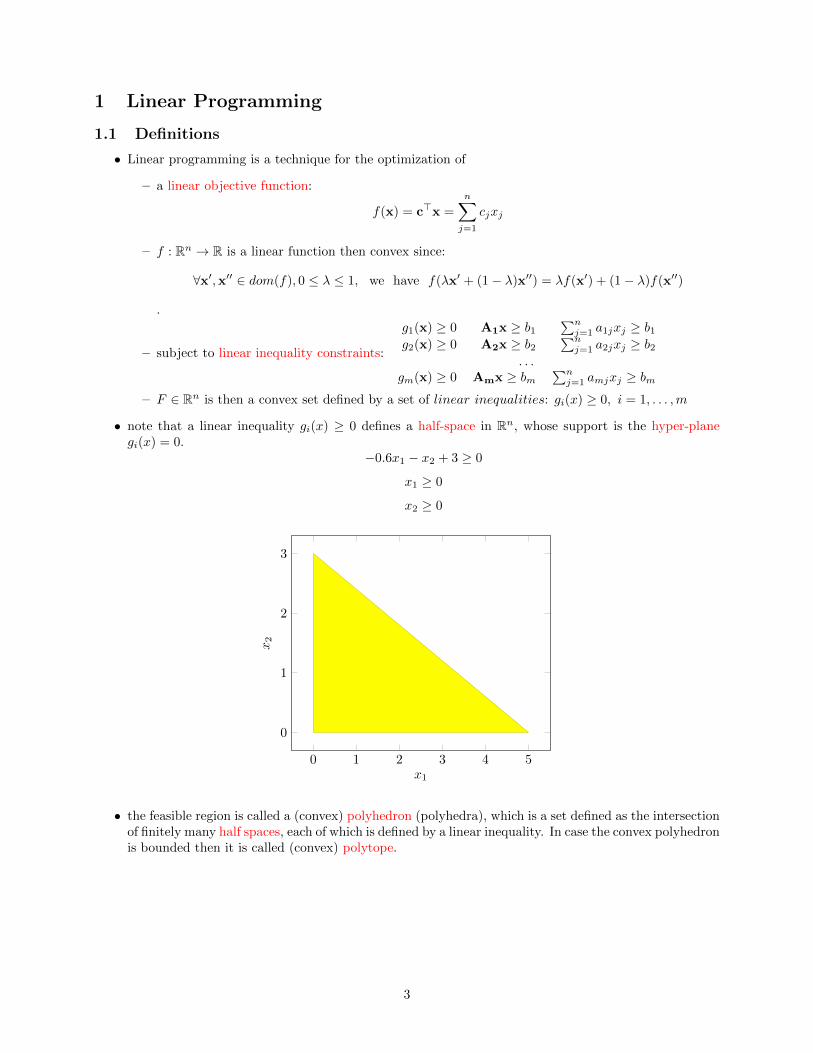
• note that a linear inequality gi(x) ≥ 0 defines a half-space in Rn, whose support is the hyper-planegi(x) = 0.

−0.6x1 − x2 + 3 ≥ 0

x1 ≥ 0

x2 ≥ 0

0 1 2 3 4 5

0

1

2

3

x1

x2

• the feasible region is called a (convex) polyhedron (polyhedra), which is a set defined as the intersectionof finitely many half spaces, each of which is defined by a linear inequality. In case the convex polyhedronis bounded then it is called (convex) polytope.

3

Example of 2D Polytope

+x1 − x2 ≥ −2

−8x1 − 2x2 ≥ −19

x1, x2 ≥ 0

x1

x2

3.5

1.5

2

2.375

(x1 = 0, x2 = 2)(x1 = 1.5, x2 = 3.5)

(x1 = 1.5, x2 = 3.5)(x1 = 2.375, x2 = 0)

Example of 2D Polyhedron

x1 + x2 ≥ 2

−x1 + x2 ≥ 0

x1, x2 ≥ 0

x1

x2

2

1

1

(x1 = 0, x2 = 2)(x1 = 1, x2 = 1)

(x1 = 1, x2 = 1)(x1 = 0, x2 = 0)

• The objective function is a real-valued affine (linear) function defined on a polyhedron (An affinefunction is a function composed of a linear function plus a constant).

Example of objective function f(x1, x2) = x1 + 2x2:

x1

x2

∇f(x1, x2) =[1 2

]contours of f(x1, x2)

f(x1, x2) = 8f(x1, x2) = 4f(x1, x2) = 21

2

4

1 2 4 8

• A linear programming algorithm finds a point in the polyhedron where this function has the smallest(or largest) value if such a point exists.

Example of 3D Polytope

4

0

1

2

0 0.5 1 1.5 2

0

2

1.2 Notation

Z(LP)= min c>x (1)

Ax ≥ b (2)

x ≥ 0 (3)

where A ∈ Rm·n , b ∈ Rm, c ∈ Rn.

INPUT DATA : A =

a11 a12 . . . a1na21 a22 . . . a2n. . . . . . . . . . . .am1 am2 . . . amn

b =

b1b2. . .bm

c =

c1c2. . .. . .. . .cn

VARIABLES : x =

x1x2. . .. . .. . .xn

Equivalent way an writing an LP:

Z(LP)= min

n∑j=1

cjxj (4)

n∑j=1

aijxj ≥ bi i = 1, . . . ,m (5)

xj ≥ 0 j = 1, . . . , n (6)

Example:

A =

[50 31−3 2

]b =

[2504

]c =

[1

0.64

]x =

[x1x2

] Z(LP) = max x1 + 0.64x250x1 + 31x2 ≤ 250−3x1 + 2x2 ≤ 4x1, x2 ≥ 0

5

x1

x2

(0, 2)

x∗2 = 950193 ≈ 4.92

x∗1 = 376193 ≈ 1.94

Z(LP)= 984193 ≈ 5.09

∇f(x) =[1 0.64

](5, 0)

(0, 25031 ≈ 8.064)

• the optimal solution value is Z(LP)= 984193 ≈ 5.09

• the optimal solution x∗ =

[376193

950193

]

• a feasible (suboptimal) solution is x =

[50

]and its corresponding solution value is 5

Canonical (n variables and m inequalities constraints) and standard (n+m variables and mequalities constraints) forms

Z(LP)= min

n∑j=1

cjxj

n∑j=1

aijxj ≥ bi i = 1, . . . ,m

xj ≥ 0 j = 1, . . . , n

Z(LP)= min

n∑j=1

cjxj

n∑j=1

aijxj−si=bi i = 1, . . . ,m

xj ≥ 0 j = 1, . . . , n

si≥ 0 i = 1, . . . ,m

• to transform a problem from the Canonical to the Standard form is it necessary to add m (non-negative)slack variables (one for each inequality) in order to transform inequalities into equalities.

• Negative variable: if xi < 0, we can define x′i ≥ 0 such that xi = −x′i

• Free variable: if xi R 0, we can define x+i , x−i ≥ 0 such that xi = x+i − x

−i

6

•min f(x) = −max−f(x)

•min f(x) + k = k + min f(x)

•min k · f(x) = k ·min f(x) with k ≥ 0

•min−k · f(x) = −k ·max f(x) with k ≥ 0

• Equalities can be transformed into inequalities constraints:

n∑j=1

aijxj = bi ⇒n∑j=1

aijxj ≤ bi,n∑j=1

aijxj ≥ bi

1.3 Example

• Consider a company which produces a metal tube and wants to plan the production for the next fourweeks in order to satisfy the demand (d, [m]) of 45.50, 58.70, 75.90 and 24.60 (each week respectively).

• The company has an initial available quantity (p0, [m]) of 11.60 meters.

• Each week the company can:

– produce a max amount of 41.50 meters (p, [m]) of metal tube at a unit cost (c, [$/m]) of 400$,

– store at a unit cost (c, [$/m]) of 20$ (unlimited amount),

– buy from the market at a unit cost (c, [$/m]) of 450$ (unlimited amount).

• Write an LP model to plan the production at the minimum cost.

Decision variables:

• xt = meters of metal tube produced at week t (t = 1, 2, 3, 4)

• yt = meters of metal tube bought form the market at week t (t = 1, 2, 3, 4)

• st = quantity stored at period t (t = 0, 1, 2, 3, 4), s0 = 11.6

Z(LP)= min c

4∑t=1

xt + c

4∑t=1

yt + c

4∑t=1

st

xt ≤ p i = 1, . . . , 4

xt + yt + st−1 − st = dt i = 1, . . . , 4

s0=p0

xt, yt, st≥ 0 i = 1, . . . , 4

7

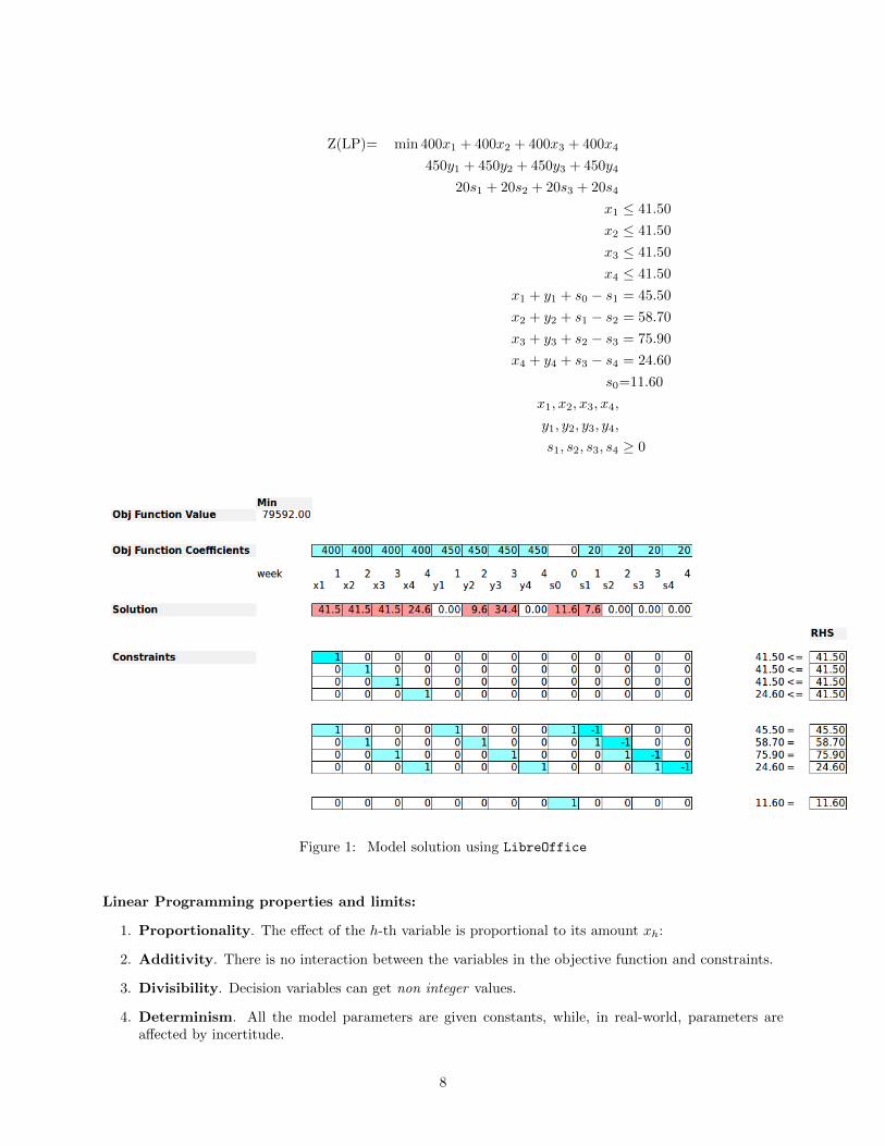
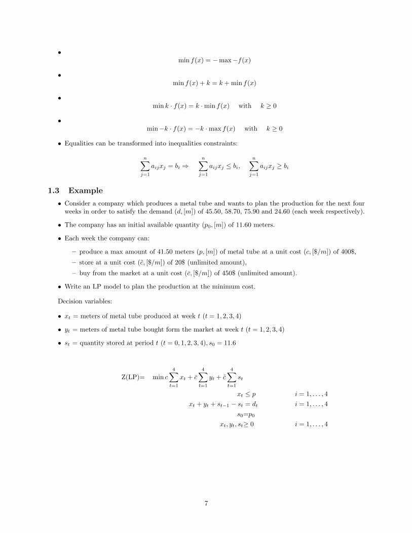
Z(LP)= min 400x1 + 400x2 + 400x3 + 400x4

450y1 + 450y2 + 450y3 + 450y4

20s1 + 20s2 + 20s3 + 20s4

x1 ≤ 41.50

x2 ≤ 41.50

x3 ≤ 41.50

x4 ≤ 41.50

x1 + y1 + s0 − s1 = 45.50

x2 + y2 + s1 − s2 = 58.70

x3 + y3 + s2 − s3 = 75.90

x4 + y4 + s3 − s4 = 24.60

s0=11.60

x1, x2, x3, x4,

y1, y2, y3, y4,

s1, s2, s3, s4 ≥ 0

Figure 1: Model solution using LibreOffice

Linear Programming properties and limits:

1. Proportionality. The effect of the h-th variable is proportional to its amount xh:

2. Additivity. There is no interaction between the variables in the objective function and constraints.

3. Divisibility. Decision variables can get non integer values.

4. Determinism. All the model parameters are given constants, while, in real-world, parameters areaffected by incertitude.

8

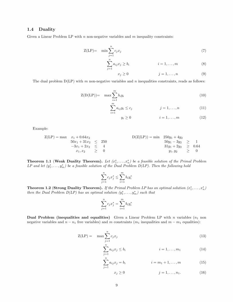
1.4 Duality

Given a Linear Problem LP with n non-negative variables and m inequality constraints:

Z(LP)= min

n∑j=1

cjxj (7)

n∑j=1

aijxj ≥ bi i = 1, . . . ,m (8)

xj ≥ 0 j = 1, . . . , n (9)

The dual problem D(LP) with m non-negative variables and n inequalities constraints, reads as follows:

Z(D(LP))= max

m∑i=1

biyi (10)

m∑i=1

aijyi ≤ cj j = 1, . . . , n (11)

yi ≥ 0 i = 1, . . . ,m (12)

Example:

Z(LP) = max x1 + 0.64x250x1 + 31x2 ≤ 250−3x1 + 2x2 ≤ 4x1, x2 ≥ 0

D(Z(LP)) = min 250y1 + 4y250y1 − 3y2 ≥ 131y1 + 2y2 ≥ 0.64y1, y2 ≥ 0

Theorem 1.1 (Weak Duality Theorem). Let (x∗1, . . . , x∗n) be a feasible solution of the Primal Problem

LP and let (y∗1 , . . . , y∗m) be a feasible solution of the Dual Problem D(LP). Then the following hold

n∑j=1

cjx∗j ≤

m∑i=1

biy∗i

Theorem 1.2 (Strong Duality Theorem). If the Primal Problem LP has an optimal solution (x∗1, . . . , x∗n)

then the Dual Problem D(LP) has an optimal solution (y∗1 , . . . , y∗m) such that

n∑j=1

cjx∗j =

m∑i=1

biy∗i

Dual Problem (inequalities and equalities) Given a Linear Problem LP with n variables (n1 nonnegative variables and n− n1 free variables) and m constraints (m1 inequalities and m−m1 equalities):

Z(LP) = max

n∑j=1

cjxj (13)

n∑j=1

aijxj ≤ bi i = 1, . . . ,m1 (14)

n∑j=1

aijxj = bi i = m1 + 1, . . . ,m (15)

xj ≥ 0 j = 1, . . . , n1. (16)

9

The dual problem D(LP) with m variables (m1 non negative variables and m − m1 free variables) and nconstraints (n1 inequalities and n− n1 equalities), reads as follows:

Z(D(LP)) = min

m∑i=1

biyi (17)

m∑i=1

aijyi ≥ cj j = 1, . . . , n1 (18)

m∑i=1

aijyi = cj j = n1 + 1, . . . , n (19)

yi ≥ 0 i = 1, . . . ,m1. (20)

1.5 LP optimality conditions

Theorem 1.3. A feasible solution (x∗1, . . . , x∗n) of the Primal Problem P is optimal if and only if there are

numbers (y∗1 , . . . , y∗m) such that

m∑i=1

aijy∗i = cj whenever x∗j > 0

y∗i = 0 whenever

n∑j=1

aijx∗j < bi

and such that

m∑i=1

aijy∗i ≥ cj forall j = 1, . . . , n

y∗i ≥ 0 forall i = 1, . . . ,m.

Example with n = 2 and m = 2:

Z(LP) = max x1 + 0.64x250x1 + 31x2 ≤ 250−3x1 + 2x2 ≤ 4x1, x2 ≥ 0

A =

[50 31−3 2

]b =

[2504

]c =

[1

0.64

]x =

[x1x2

]

• Feasible solution: x∗ =

[376193

950193

]optimal?

• y∗i = 0 if∑nj=1 aijx

∗j < bi

{50 · 376193 + 31 · 950193 = 250

−3 · 376193 + 2 · 950193 = 4−→ no y variables set to 0

•∑mi=1 aijy

∗i = cj if x∗j > 0

{50y1 − 3y2 = 1

31y1 + 2y2 = 0.64y∗ =

[98

4825

1193

]• y∗i ≥ 0 forall i = 1, . . . ,m −→ OK

•∑mi=1 aijy

∗i ≥ cj forall j = 1, . . . , n

{50 · 98

4825 − 3 · 1193 = 1

31 · 984825 + 2 · 1

193 = 0.64−→ Optimal

10

• Feasible solution: x∗ =

[0

2

]optimal?

• y∗i = 0 if∑nj=1 aijx

∗j < bi

{50 · 0 + 31 · 2 = 62

−3 · 0 + 2 · 2 = 4−→ y1 = 0

•∑mi=1 aijy

∗i = cj if x∗j > 0

{31y1 + 2y2 = 0.64

y1 = 0y∗ =

[0

0.32

]• y∗i ≥ 0 forall i = 1, . . . ,m −→ OK

•∑mi=1 aijy

∗i ≥ cj forall j = 1, . . . , n

{50 · 0− 3 · 0.32 = −0.96

31 · 0 + 2 · 0.32 = 0.64−→ Not Optimal

11

2 Integer Linear Programming

2.1 Definitions and notations

An integer linear program is a linear program with the additional constraint that the variables are requiredto be integer.

Z(ILP)= min c>x (21)

Ax ≥ b (22)

x ∈ Z+ (23)

where A ∈ Rm·n , b ∈ Rm, c ∈ Rn.

INPUT DATA : A =

a11 a12 . . . a1na21 a22 . . . a2n. . . . . . . . . . . .am1 am2 . . . amn

b =

b1b2. . .bm

c =

c1c2. . .. . .. . .cn

VARIABLES : x =

x1x2. . .. . .. . .xn

Equivalent way an writing an ILP:

Z(ILP)= min

n∑j=1

cjxj (24)

n∑i=1

aijxj ≥ bi i = 1, . . . ,m (25)

xj ∈ Z+ j = 1, . . . , n (26)

• Z(LP) is a valid bound for Z(ILP):

– lower bound in case of minimization

– upper bound in case of maximization

• Definition: ∀y ∈ R, the integer part of y is byc =max integer q : q ≤ y

• if cj ∈ Z (∀j = 1, . . . , n):

– for minimization bZ(LP )c+ 1 is a valid lower bound for Z(ILP)

– for maximization bZ(LP )c is a valid upper bound for Z(ILP)

Example:

A =

[50 31−3 2

]b =

[2504

]c =

[1

0.64

]x =

[x1x2

] Z(ILP) = max x1 + 0.64x250x1 + 31x2 ≤ 250−3x1 + 2x2 ≤ 4x1, x2 ∈ Z+

• the optimal LP solution value is Z(LP)= 984193 ≈ 5.09

• Z(LP) is an upper bound for Z(ILP) −→ upper bound = 984193 ≈ 5.09

12

x1

x2

(0, 2)

x∗2 = 950193 ≈ 4.92

x∗1 = 376193 ≈ 1.94

Z(LP)= 984193 ≈ 5.09

∇f(x) =[1 0.64

](5, 0)

(0, 25031 ≈ 8.064)

Z(ILP)=5

• bZ(LP )c is an upper bound for Z(ILP) −→ upper bound =5

• the optimal LP solution x∗LP =

[376193

950193

]−→ very far from the optimal integer solution

• the optimal solution value is Z(ILP)=5

• the optimal solution x∗ =

[5

0

]

Definition – Mixed Integer Linear Program (MILP)An ILP when some variables are restricted to be integer and some are not, the problem is called: mixedinteger linear program.

Z(MILP)= min c>x (27)

Ax ≥ b (28)

x ≥ 0 (29)

xj ∈ Z+ j = 1, . . . , p (30)

Definition – Binary program (BP)An ILP where the integer variables are restricted to be 0 or 1 (it comes up surprisingly often). Such problemsare called pure (mixed) 0–1 linear programs or pure (mixed) binary integer linear programs.

Z(BP)= min c>x (31)

Ax ≥ b (32)

x ∈ {0, 1} (33)

13

Modeling PotentialModeling with integer variables is useful in a wide variety of applications and in many financial applica-tion/problems:

• model managerial decisions

• select among different resources

• allocate scarce resources

• manage portfolios and projects

• model fixed costs

• model logical requirements (boolean conditions)

• many others . . .

2.2 Solvers

Many SOLVERs are available to direct tackle ILP problems.

Prototyping:

• EXCEL

• Libre Office

Commercial solvers:

• IBM ILOG CPLEX

• GUROBI

• XPRESS

Open source solvers:

• SCIP

• CBC

• GLPK

• LPSOLVE

Problems with more than a few thousand variables are often not possible to solve unless they show aspecific exploitable structure.

They implement Exact Algorithms based on the following techniques:

• Branch and Bound

• Cutting planes

• Branch and Cut

• Branch and Price

• A combination of the above methods

14

max f(x)

Feasible D(LP) solutions

Feasible LP solutions

Optimal solution value – Z(ILP)

Optimal LP solution value – Z(LP)=Z(D(LP)) Upper Bound

Feasible integer solution value – Z(x) Lower Bound

Feasible integer solution value – Z(x) Lower Bound

min f(x)

Feasible LP solutions

Feasible D(LP) solutions

Optimal solution value – Z(ILP)

Optimal LP solution value – Z(LP)=Z(D(LP)) Lower Bound

Feasible integer solution value – Z(x) Upper Bound

Feasible integer solution value – Z(x) Upper Bound

Relaxations and feasible solutions (for maximization and minimization problems)

2.3 Example

Example 1 Suppose we wish to invest 19,000 e and we have four investment opportunities:

1 investment of 6,700 e and has a net present value of 8,000 e

2 investment of 10,000 e and has a net present value of 11,000 e

15

3 investment of 5,500 e and has a net present value of 6,000 e

4 investment of 3,400 e and has a net present value of 4,000 e

Into which investments should we place our money so as to maximize our total present value? Suchproblems are called capital budgeting problems.

Decision variables:

xj =

{1 if investment j is made (j = 1, . . . , 4)0 otherwise

max 8, 000x1 + 11, 000x2 + 6, 000x3 + 4, 000x4 (34)

6, 700x1 + 10, 000x2 + 5.500x3 + 3, 400x4 ≤ 19, 000 (35)

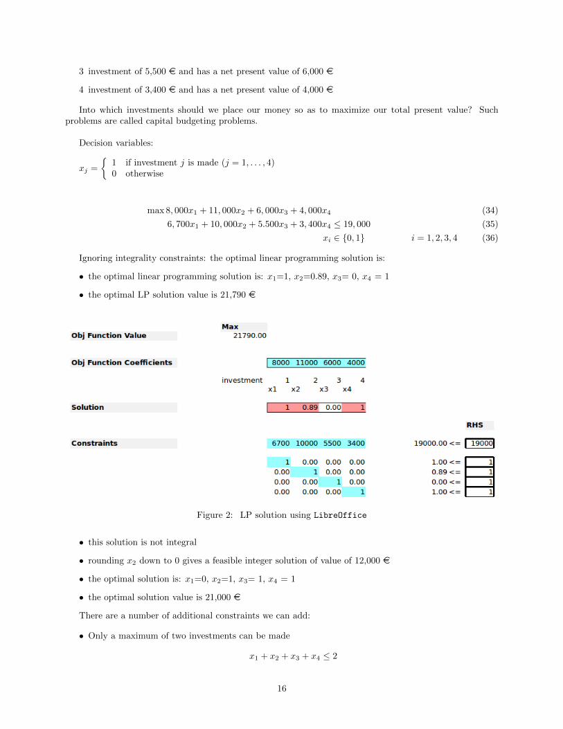
xi ∈ {0, 1} i = 1, 2, 3, 4 (36)

Ignoring integrality constraints: the optimal linear programming solution is:

• the optimal linear programming solution is: x1=1, x2=0.89, x3= 0, x4 = 1

• the optimal LP solution value is 21,790 e

Figure 2: LP solution using LibreOffice

• this solution is not integral

• rounding x2 down to 0 gives a feasible integer solution of value of 12,000 e

• the optimal solution is: x1=0, x2=1, x3= 1, x4 = 1

• the optimal solution value is 21,000 e

There are a number of additional constraints we can add:

• Only a maximum of two investments can be made

x1 + x2 + x3 + x4 ≤ 2

16

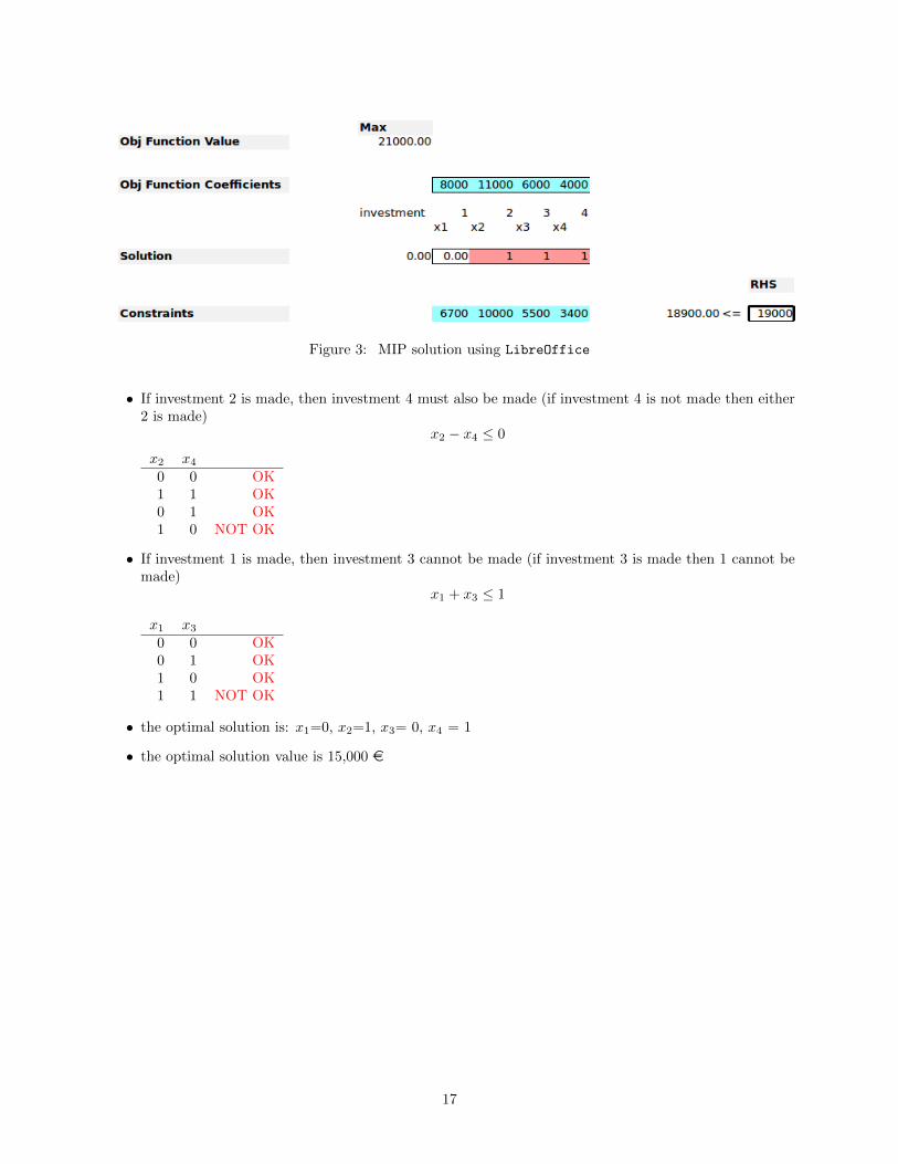
Figure 3: MIP solution using LibreOffice

• If investment 2 is made, then investment 4 must also be made (if investment 4 is not made then either2 is made)

x2 − x4 ≤ 0

x2 x40 0 OK1 1 OK0 1 OK1 0 NOT OK

• If investment 1 is made, then investment 3 cannot be made (if investment 3 is made then 1 cannot bemade)

x1 + x3 ≤ 1

x1 x30 0 OK0 1 OK1 0 OK1 1 NOT OK

• the optimal solution is: x1=0, x2=1, x3= 0, x4 = 1

• the optimal solution value is 15,000 e

17

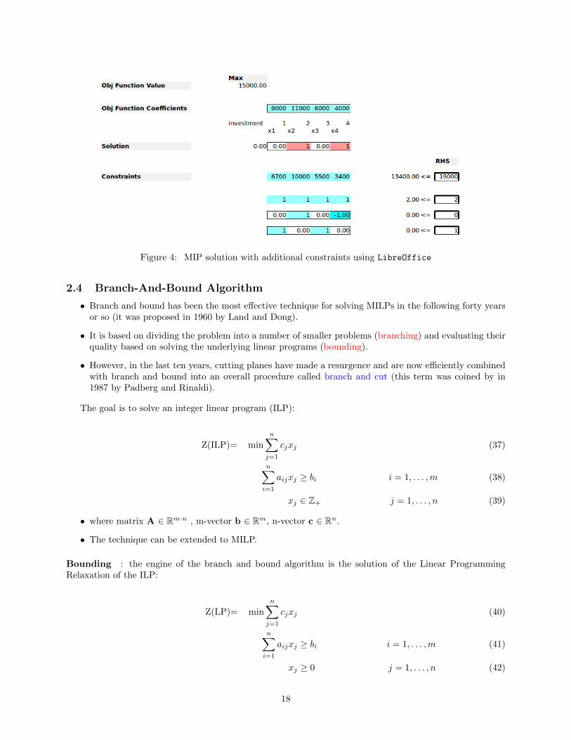
Figure 4: MIP solution with additional constraints using LibreOffice

2.4 Branch-And-Bound Algorithm

• Branch and bound has been the most effective technique for solving MILPs in the following forty yearsor so (it was proposed in 1960 by Land and Dong).

• It is based on dividing the problem into a number of smaller problems (branching) and evaluating theirquality based on solving the underlying linear programs (bounding).

• However, in the last ten years, cutting planes have made a resurgence and are now efficiently combinedwith branch and bound into an overall procedure called branch and cut (this term was coined by in1987 by Padberg and Rinaldi).

The goal is to solve an integer linear program (ILP):

Z(ILP)= min

n∑j=1

cjxj (37)

n∑i=1

aijxj ≥ bi i = 1, . . . ,m (38)

xj ∈ Z+ j = 1, . . . , n (39)

• where matrix A ∈ Rm·n , m-vector b ∈ Rm, n-vector c ∈ Rn.

• The technique can be extended to MILP.

Bounding : the engine of the branch and bound algorithm is the solution of the Linear ProgrammingRelaxation of the ILP:

Z(LP)= min

n∑j=1

cjxj (40)

n∑i=1

aijxj ≥ bi i = 1, . . . ,m (41)

xj ≥ 0 j = 1, . . . , n (42)

18

• The best known (and most successful) methods for solving LPs is the simplex algorithm.

• Rounding the solution of the LP will not in general give the optimal solution of the ILP.

• Since the the LP is less constrained than an ILP, the following are immediate:

– The optimal objective value for the LP is less than or equal to the optimal objective for the ILP

– If the LP is infeasible, then so is ILP

– If the optimal solution x∗ of the LP satisfies x∗i integer for i = 1, ..., n, then x∗ is also optimal forthe ILP

– Otherwise, it gives a bound on the optimal value of the ILP

Notation and data structure

• The branch-and-bound algorithm keeps a list of linear programming problems obtained by relaxing theintegrality requirements on the variables and imposing constraints such as:

– xj ≤ uj– xj ≥ lj

• Each such linear program corresponds to a node of the branch-and-bound tree.

• For a node Ni , let Z(Ni) denote the optimal solution value of the corresponding linear program.

• Let L denote the list of nodes that must still be solved.

• Let ZB denote a valid bound on the optimum value (initially, the bound ZB can be derived from aheuristic solution of MILP, or it can be set to +∞).

Pseudo code of the algorithm

Step 0 Initialize L = ILP, ZB = +∞, x∗ = ∅.

Step 1 Terminate? If L = ∅, the solution x∗ is optimal.

Step 2 Select node Choose and delete a problem Ni from L.

Step 3 Bound Solve Ni . If it is infeasible, go to Step 1. Else, let xi be its solution and Z(Ni) its objectivevalue.

Step 4 Prune

– If Z(Ni) ≥ ZB , go to Step 1.

– If xi is not feasible for MILP, go to Step 5.

– If xi is feasible for ILP, let ZB = Z(Ni) , x∗ = xi. Delete from L all problems with Z(Nj) ≥ ZB .Go to Step 1.

Step 5 Branch From Ni , construct linear programs N1i , . . . , N

ki with smaller feasible regions whose union

contains all the feasible solutions of (MILP) in Ni . Add N1i , . . . , N

ki to L and go to Step 1.

We can stop the enumeration at a node of the branch-and-bound tree for three different reasons (whenthey occur, the node is said to be pruned).

• Pruning by integrality occurs when the corresponding linear program has an optimum solution thatis integral.

• Pruning by bounds occurs when the objective value of the linear program at that node is worse thanthe value of the best feasible solution found so far.

• Pruning by infeasibility occurs when the linear program at that node is infeasible.

19

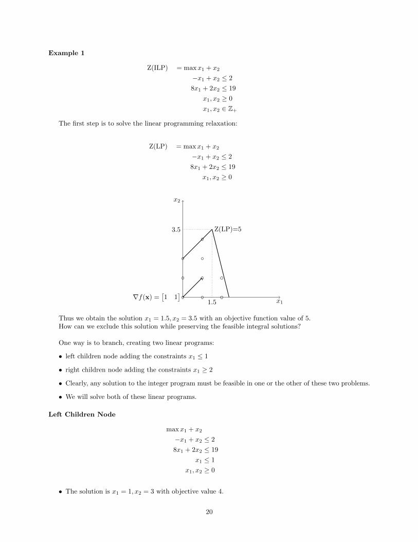
Example 1

Z(ILP) = maxx1 + x2

−x1 + x2 ≤ 2

8x1 + 2x2 ≤ 19

x1, x2 ≥ 0

x1, x2 ∈ Z+

The first step is to solve the linear programming relaxation:

Z(LP) = maxx1 + x2

−x1 + x2 ≤ 2

8x1 + 2x2 ≤ 19

x1, x2 ≥ 0

x1

x2

Z(LP)=53.5

1.5∇f(x) =

[1 1

]Thus we obtain the solution x1 = 1.5, x2 = 3.5 with an objective function value of 5.How can we exclude this solution while preserving the feasible integral solutions?

One way is to branch, creating two linear programs:

• left children node adding the constraints x1 ≤ 1

• right children node adding the constraints x1 ≥ 2

• Clearly, any solution to the integer program must be feasible in one or the other of these two problems.

• We will solve both of these linear programs.

Left Children Node

maxx1 + x2

−x1 + x2 ≤ 2

8x1 + 2x2 ≤ 19

x1 ≤ 1

x1, x2 ≥ 0

• The solution is x1 = 1, x2 = 3 with objective value 4.

20

x1

x2

3

1∇f(x) =

[1 1

]

• This is a feasible integral solution.

• So we now have an upper bound of 5 as well as a lower bound of 4 on the value of an optimum solutionto the integer program.

Right Children Node

maxx1 + x2

−x1 + x2 ≤ 2

8x1 + 2x2 ≤ 19

x1 ≥ 2

x1, x2 ≥ 0

x1

x2

1.5

2∇f(x) =

[1 1

]

• The solution is x1 = 2, x2 = 1.5 with objective value 3.5.

• Because this value is worse that the lower bound of 4 that we already have, we do not need any furtherbranching.

• We conclude that the feasible integral solution of value 4 found earlier is optimum.

These problems can be arranged in a branch-and-bound tree. Each node of the tree corresponds toone of the problems that were solved:

21

Figure 5: B&B tree of example 1

Example 2

Z(ILP) = max 3x1 + x2

−x1 + x2 ≤ 2

8x1 + 2x2 ≤ 19

x1, x2 ≥ 0

x1, x2 ∈ Z+

Figure 6: B&B tree of example 2

Point of intersection (α, β) = ( c·s−b·tb·r−a·s ,a·t−c·rb·r−a·s ) among two lines:{

a · x1 + b · x2 + c = 0r · x1 + s · x2 + t = 0

22

3 Construction of an Index Fund

Different possibilities of portfolio management:

• active portfolio management tries to achieve superior performance by using forecasting techniques

• passive portfolio management avoids any forecasting techniques and rather relies on diversificationto achieve a desired performance

There are 2 types of passive management strategies:

• buy and hold: assets are selected on the basis of some fundamental criteria and there is no activeselling or buying of these stocks afterwards

• indexing: the goal is to choose a portfolio that mirrors the movements of a broad market populationor a market index. Such a portfolio is called an index fund.

Index fund – Definition Given a target population of n stocks, one selects q stocks and their weights inthe index fund, to represent the target population as closely as possible.

In the last twenty years, an increasing number of investors, both large and small, have established indexfunds. The rising popularity of index funds can be justified both theoretically and empirically:

• Market Efficiency: If the market is efficient, no superior risk-adjusted returns can be achieved bystock picking strategies since the prices reflect all the information available in the marketplace. Anindex fund captures the efficiency of the market via diversification.

• Empirical Performance: Considerable empirical literature provides strong evidence that, on average,money managers have consistently underperformed the major indexes (luck is an explanation for goodperformance).

• Transaction Cost: Actively managed funds incur transaction costs, which reduce the overall perfor-mance of these funds. In addition, active management implies significant research costs.

Additional features:

• Here we take the point of view of a fund manager who wants to construct an index fund.

• Strategies for forming index funds involve choosing a broad market index as a proxy for an entiremarket, e.g. the Standard and Poor list of 500 stocks (S&P 500)

• A pure indexing approach consists in purchasing all the issues in the index, with the same exact weightsas in the index.

• In most instances, this approach is impractical (many small positions) and expensive (rebalancing costsmay be incurred frequently)

A Large-Scale Deterministic Model

• We propose a large-scale deterministic model for aggregating a broad market index of stocks into asmaller more manageable index fund.

• This approach will produce a portfolio that closely replicates the underlying market population.

We present a model that:

• clusters the assets into groups of similar assets

• selects one representative asset from each group to be included in the index fund portfolio

23

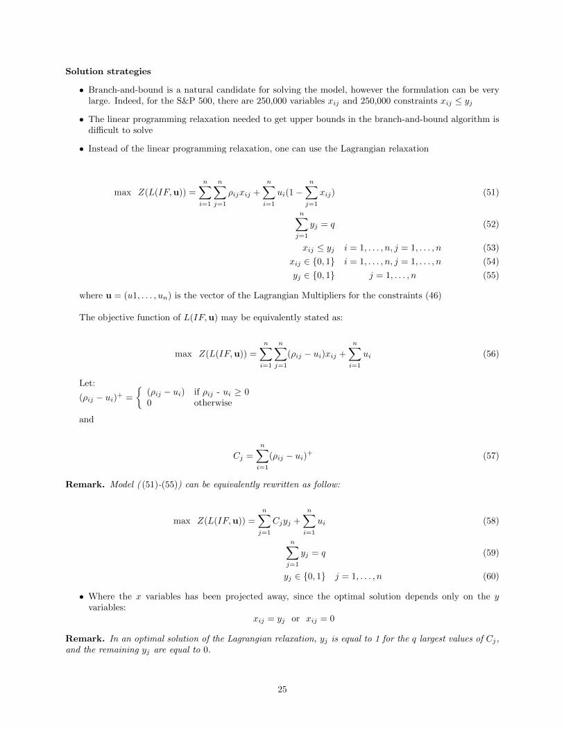
The model is based on the following data:

ρij = similarity between stock i and stock j (43)

Typical features:

• ρii = 1

• ρij ≤ 1 for i 6= j

• ρij is larger for more similar stocks

• An example of this is the correlation between the returns of stocks i and j

Decision variables:

yj =

{1 if stock j is in the index fund0 otherwise

xij =

{1 if j is the most similar stock to stock i in the index fund0 otherwise

max Z(IF ) =

n∑i=1

n∑j=1

ρijxij (44)

n∑j=1

yj = q (45)

n∑j=1

xij = 1 i = 1, . . . , n (46)

xij ≤ yj i = 1, . . . , n, j = 1, . . . , n (47)

xij ∈ {0, 1} i = 1, . . . , n, j = 1, . . . , n (48)

yj ∈ {0, 1} j = 1, . . . , n (49)

• Interpret each of the constraints

• Explain why the objective of the model can be interpreted as selecting q stocks out of the populationof n stocks so that the total loss of information is minimized

Once the model has been solved and a set of q stocks has been selected for the index fund, a weight wjis calculated for each j in the fund:

wj =

n∑i=1

Vixij (50)

where Vi is the market value of stock i.

• So wj is the total market value of the stocks represented by stock j in the fund

• The fraction of the index fund to be invested in stock j is proportional to the stocks weight wj

• wj∑qf=1 wf

• Note that, instead of the objective function used, one could have used an objective function that takesthe weights wj directly into account

∑ni=1

∑nj=1 Viρijxij

24

Solution strategies

• Branch-and-bound is a natural candidate for solving the model, however the formulation can be verylarge. Indeed, for the S&P 500, there are 250,000 variables xij and 250,000 constraints xij ≤ yj

• The linear programming relaxation needed to get upper bounds in the branch-and-bound algorithm isdifficult to solve

• Instead of the linear programming relaxation, one can use the Lagrangian relaxation

max Z(L(IF,u)) =

n∑i=1

n∑j=1

ρijxij +

n∑i=1

ui(1−n∑j=1

xij) (51)

n∑j=1

yj = q (52)

xij ≤ yj i = 1, . . . , n, j = 1, . . . , n (53)

xij ∈ {0, 1} i = 1, . . . , n, j = 1, . . . , n (54)

yj ∈ {0, 1} j = 1, . . . , n (55)

where u = (u1, . . . , un) is the vector of the Lagrangian Multipliers for the constraints (46)

The objective function of L(IF,u) may be equivalently stated as:

max Z(L(IF,u)) =

n∑i=1

n∑j=1

(ρij − ui)xij +

n∑i=1

ui (56)

Let:

(ρij − ui)+ =

{(ρij − ui) if ρij - ui ≥ 00 otherwise

and

Cj =

n∑i=1

(ρij − ui)+ (57)

Remark. Model ( (51)-(55)) can be equivalently rewritten as follow:

max Z(L(IF,u)) =

n∑j=1

Cjyj +

n∑i=1

ui (58)

n∑j=1

yj = q (59)

yj ∈ {0, 1} j = 1, . . . , n (60)

• Where the x variables has been projected away, since the optimal solution depends only on the yvariables:

xij = yj or xij = 0

Remark. In an optimal solution of the Lagrangian relaxation, yj is equal to 1 for the q largest values of Cj,and the remaining yj are equal to 0.

25

• Once the optimal solution in term of the y variables has been computed then the x variables can becomputed: xij = 1 if ρij - ui ≥ 0 and yj = 1 (0 otherwise).

• it worth mentioning that in the solution of the Lagrangian relaxation more one stock i can be assignedto each stock j in the index fund (or zero).

• Interestingly, the set of q stocks corresponding to the q largest values of Cj can also be used to build aheuristic solution for the model IF. Specifically, construct an index fund containing these q stocks andassign each stock i = 1, . . . , n to the most similar stock in this fund. This solution is feasible to themodel, although not necessarily optimal.

• So for any vector u, we can compute quickly both a lower bound and an upper bound on the optimumvalue of the model IF.

How does one minimize L(IF,u)?

• Since L(u) is non-differentiable and convex, one can use the subgradient method

• At each iteration, a revised set of Lagrange multipliers u and an accompanying lower bound and upperbound to the model are computed

• At each iteration constraints (46) can be violated (some stock can be assigned to more than one stockor to zero). Accordingly a sub-gradient optimisation method can be used (See the appendix for furtherdetails).

• The algorithm terminates when these two bounds match or when a maximum number of iterations isreached

• It can be proven that min Z(L(IF,u)) is equal to the optimal value of model IF , i.e., Z(IF ).

• To solve the integer program to optimality, one can also use a branch-and-bound algorithm, using asupper bound Z(L(IF,u)) for pruning the nodes.

26

4 Portfolio Selection and Asset Allocation

• The theory of optimal selection of portfolios was developed by Harry Markowitz in the 1950s

• His work formalized the diversification principle in portfolio selection

• Key assumption: Trades off between expected returns and the perceived risk of portfolios.

4.1 Preliminaries and Notation

• Consider a set of rates of return rti (t = 1, . . . , T, i = 1, . . . , n)

• The value rti represents the rate of return of a security i at time t

• T represents the temporal horizon under consideration and n is the number of securities

• Starting from the time series of the rates of return we can compute:

arithmetic mean

rai =1

T

T∑t=1

rti

geometric mean (only positive values)

rgi = (

T∏t=1

(1 + rti))1T − 1

Since the rates of returns are typically not smaller than 1 is it sufficient to add 1 in order to get positivevalues (then shift back subtracting 1).

Example with 2 rates of returns and a specific security i:

rai rgi-1 1 0.0 -1-1 0 -0.5 -10 1 0.5 0.410 0 0.0 0.0

-0.5 0.5 0.0 -0.130.1 0.25 0.18 0.17

Table 1: Arithmetic and geometric means

variance

σ2i =

1

T

T∑t=1

(rti − rai )2

standard deviation

σi =

√√√√ 1

T

T∑t=1

(rti − rai )2

27

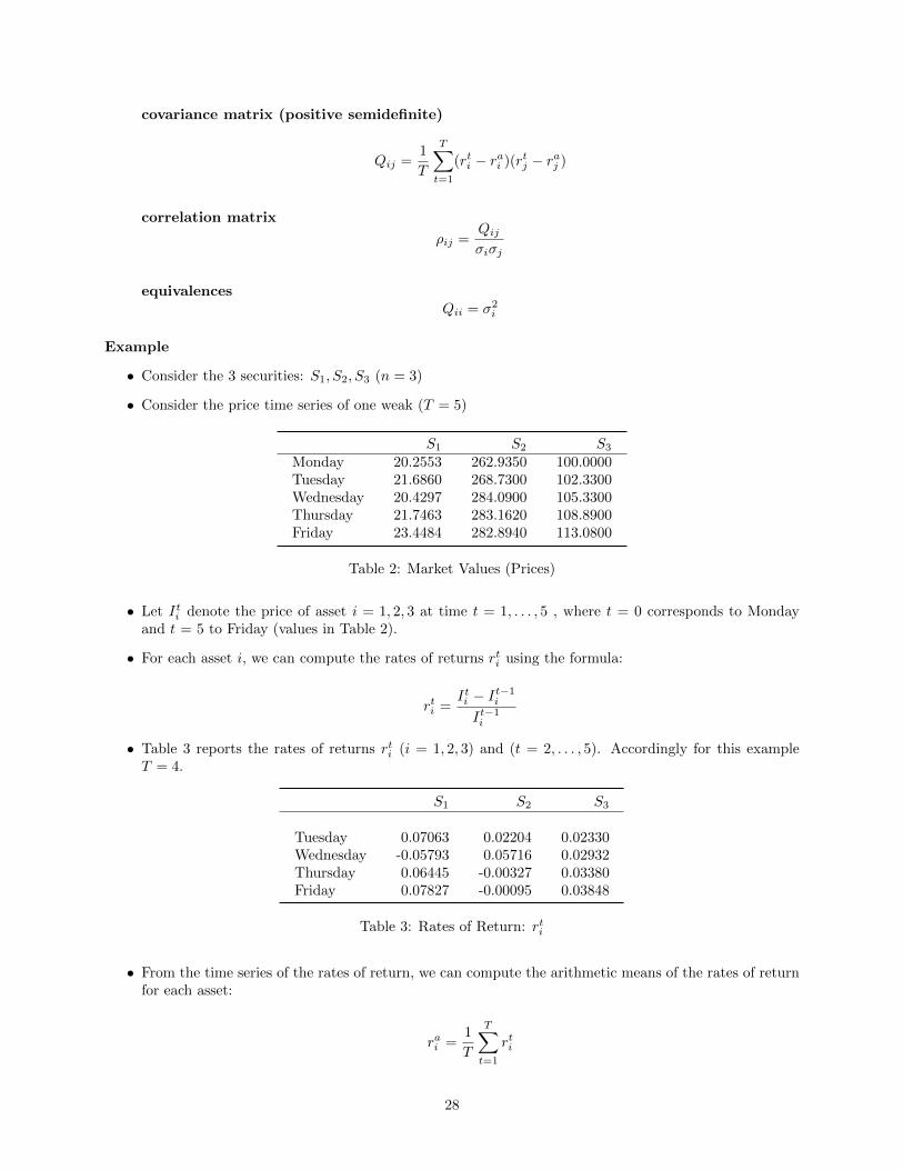
covariance matrix (positive semidefinite)

Qij =1

T

T∑t=1

(rti − rai )(rtj − raj )

correlation matrix

ρij =Qijσiσj

equivalencesQii = σ2

i

Example

• Consider the 3 securities: S1, S2, S3 (n = 3)

• Consider the price time series of one weak (T = 5)

S1 S2 S3

Monday 20.2553 262.9350 100.0000Tuesday 21.6860 268.7300 102.3300Wednesday 20.4297 284.0900 105.3300Thursday 21.7463 283.1620 108.8900Friday 23.4484 282.8940 113.0800

Table 2: Market Values (Prices)

• Let Iti denote the price of asset i = 1, 2, 3 at time t = 1, . . . , 5 , where t = 0 corresponds to Mondayand t = 5 to Friday (values in Table 2).

• For each asset i, we can compute the rates of returns rti using the formula:

rti =Iti − I

t−1i

It−1i

• Table 3 reports the rates of returns rti (i = 1, 2, 3) and (t = 2, . . . , 5). Accordingly for this exampleT = 4.

S1 S2 S3

Tuesday 0.07063 0.02204 0.02330Wednesday -0.05793 0.05716 0.02932Thursday 0.06445 -0.00327 0.03380Friday 0.07827 -0.00095 0.03848

Table 3: Rates of Return: rti

• From the time series of the rates of return, we can compute the arithmetic means of the rates of returnfor each asset:

rai =1

T

T∑t=1

rti

28

S1 S2 S3

rai 0.03885 0.01875 0.03122

Table 4: Arithmetic means of the rates of return: rai

• Table 4 reports the arithmetic means of the rates of return of the example:

• From the time series of the rates of return, we can also compute the geometric means of the rates ofreturn for each asset:

rgi = (

T∏t=1

(1 + rti))1T − 1

• Table 5 reports the geometric means of the rates of return of the example:

S1 S2 S3

rgi 0.03727 0.01846 0.03121

Table 5: Geometric means of the rates of return: rgi

• We now compute the covariance matrix:

Qij =1

T

T∑t=1

(rti − rai )(rtj − raj )

S1 S2 S3

S1 0.00315 -0.00124 0.00007S2 -0.00124 0.00059 -0.00007S3 0.00007 -0.00007 0.00003

Table 6: Covariance Matrix: Qij

• We can now compute the standard deviation (also called Volatility):

σi =

√√√√ 1

T

T∑t=1

(rti − rai )2

S1 S2 S3

σi 0.05609 0.02428 0.00561

Table 7: Standard deviation: σi

• We now compute the correlation matrix:

ρij =Qijσiσj

29

S1 S2 S3

S1 1.00000 -0.90898 0.22629S2 -0.90898 1.00000 -0.54895S3 0.22629 -0.54895 1.00000

Table 8: Correlation Matrix: ρij

4.2 Mean-variance optimization (MVO) – Markowitz portfolio optimization

• Consider now an investor who wants to invest a certain amount of money in a number of differentsecurities (stocks, bonds, etc.) with random expected returns

• For each security the price time series is available

• For each security i = 1, . . . , n, we estimates:

– the expected return µi (typically the geometric mean of the rates of return rgi )

– the variance σ2i or the standard deviation σi

• For any couple of securities i and j, we estimates:

– covariance Qij or the correlation coefficient ρij

• If we represent the proportion of the total funds invested in security i by xi, a portfolio is a vector:

x = (x1, ..., xn)

expected return of a portfolio

E[x] = x1µ1 + · · ·+ xnµn = µ>x

where:

µ =

µ1

µ2

...µn

variance of a portfolio

Var[x] =

n∑i=1

n∑j=1

Qijxixj =

n∑i=1

n∑j=1

ρijσiσjxixj = x>Qx

where:

Q =

Q11 Q12 . . . Q1n

Q21 Q22 . . . Q2n

. . . . . . . . . . . .Qn1 Qn2 . . . Qnn

• In linear algebra, a symmetric n · n real matrix M is said to be positive semidefinite:

– if the scalar xTMx is non-negative for every non-zero column vector x of n real numbers.

30

– All the eigenvalues of M are non-negative

• The covariance matrix Q is positive semidefinite:

∑i

∑j

xixjQij =∑i

∑j

xixj1

T

T∑t=1

(rti − rai )(rtj − raj ) =

1

T

T∑t=1

∑i

xi(rti − rai )

∑j

xj(rtj − raj ) =

1

T

T∑t=1

∑j

xj(rtj − raj )

(∑i

xi(rti − rai )

)=

1

T

T∑t=1

(∑i

xi(rti − rai )

)(∑i

xi(rti − rai )

)=

1

T

T∑t=1

(∑i

xi(rti − rai )

)2

≥ 0

• then for any x, x>Qx ≥ 0.

Portfolio features:

• The portfolio vector x must satisfy∑i xi = 1

• There may or may not be additional feasibility constraints

• A feasible portfolio x is called efficient if:

– it has the minimum variance among all portfolios that have at least a certain expected return

– it has the maximal expected return among all portfolios with less than a certain variance level

• The collection of efficient portfolios forms the efficient frontier of the portfolio universe

• The efficient frontier is often represented as a curve in a two-dimensional graph where the coordinatesof a plotted point corresponds to:

– the expected return

– the variance of the efficient portfolio

The MVO problem can be formulated in 2 but equivalent ways:

First formulation

• the first formulation results in the problem of finding a minimum variance portfolio of the securities 1to n that yields at least a target value R of expected return (target return).

Convex quadratic programming problem:

min x>Qx (61)

e>x = 1 (62)

µ>x ≥ R (63)

x ≥ 0 (64)

• where e is an n-dimensional vector all of which components are equal to 1

e =

11...1

31

• The first constraint indicates that the proportions xi should sum up to 1

• The second constraint indicates that the expected return is no less than the target value R

• the objective function corresponds to the total variance of the portfolio

• Nonnegativity constraints on xi are introduced to avoid short sales

• Solving this problem for values of R ranging between Rmin and Rmax one obtains all efficient portfolios

– Rmin can be set to 0 since portfolios with a negative target return can be discarded.Attention: if

maxi=1,...,n

rgi < 0

the model become infeasible

– Rmax can be set to:max

i=1,...,nrgi

since in this case the portfolio will consists only of the security i∗ with the largest geometric meanof the rates of return. Accordingly the variance of this portfolio will be the σ2

i∗

Second formulation

• the second formulation results in the problem of finding a portfolio of maximum expected return of thesecurities 1 to n that respects a maximum level of variance R.

Convex quadratically constrained programming problem:

maxµ>x (65)

e>x = 1 (66)

x>Qx ≤ R (67)

x ≥ 0 (68)

• this formulation is less used and accordingly in the rest of the section we will focus on the first formu-lation

Possible additional constraints

• the set of admissible portfolios can be a nonempty polyhedral set represented as

χ = {x : Ax = b,Cx ≥ d}

where A is an m · n matrix, b is an m-dimensional vector, C is a p · n matrix and d is a p-dimensionalvector.

• In this case it is necessary to add the following constraints to the models

Ax = b (69)

Cx ≥ b (70)

• For example, if regulations or investor preferences limit the amount of investment in a subset of thesecurities, the model can be augmented with a linear constraint to reflect such a limit.

• In principle, any linear constraint can be added to the model without making it significantly harder tosolve.

32

Markowitzs MVO model example

• We construct now the Markowitz’s MVO model to construct a portfolio of three securities: S1, S2, S3

of the previous example.

• Rmin can be set to: 0.0

Rmax can be set to: 0.03727, i.e., µ1

• For a expected target return R the QP model reads as as follows:

min 0.00315x21 + 0.00059x22 + 0.00003x23 (71)

−2 · 0.00124x1x2 + 2 · 0.00007x1x3 − 2 · 0.00007x2x3 (72)

x1 + x2 + x3 = 1 (73)

0.03727x1 + 0.01846x2 + 0.03121x3 ≥ R (74)

x1, x2, x3 ≥ 0 (75)

• Solving the model for R = 0.028 to R = 0.033 with increments of 0.1% we get the following optimalportfolios and the corresponding variance.

Target Return R Variance x1 x2 x30.028 0.000003 0.11 0.30 0.590.029 0.000006 0.08 0.21 0.720.030 0.000014 0.04 0.12 0.840.031 0.000028 0.01 0.02 0.970.032 0.000093 0.13 0.00 0.870.033 0.000320 0.30 0.00 0.70

Table 9: Efficient Portfolios

• Efficient frontier

Figure 7: Efficient frontier

33

Asset allocation

• Asset allocation problems have the same mathematical structure as portfolio selection problems.

• In these problems the objective is not to choose a portfolio of stocks (or other securities) but to determinethe optimal investment among a set of asset classes

• Examples of asset classes are large capitalization stocks, small capitalization stocks, foreign stocks,government bonds, corporate bonds, etc.

• After estimating the expected returns, variances, and covariances for different asset classes, one canformulate a Markowitz model and obtain efficient portfolios of these asset classes.

Example for the Markowitzs MVO model

• The KKT conditions are first order necessary conditions for a solution in nonlinear programming tobe optimal. Markowitz model is a convex quadratic programming problem for which the first orderconditions are both necessary and sufficient for optimality.

• A portofio x∗ is an optimal portfolio if and only if there exists ye ∈ R, yR ∈ R,yE ∈ Rm , and yI ∈ Rp

satisfying the following conditions:

−2Qx∗ = −yRµ−C>yI + ye + A>yE (Stationarity) (76)

R− µ>x∗ ≤ 0,d−Cx∗ ≤ 0 (Primal feasibility) (77)

e>x∗ − 1 = 0,Ax∗ − b = 0 (Primal feasibility) (78)

yR ≥ 0,yI ≥ 0 (Dual feasibility) (79)

yR(R− µ>x∗) = 0 (Complementary slackness) (80)

y>I (d−Cx∗) = 0 (Complementary slackness) (81)

4.3 Large-Scale Portfolio Optimization

• We consider now the practical issues that arise when the Mean- Variance model is used to construct aportfolio from a large underlying family of assets or stocks

• the number of assets or stocks n may be in the hundreds or thousands.

• Diversification – In general, there is no reason to expect that solutions to the Markowitz model will bewell diversified portfolios

• Practitioners often use additional constraints to ensure that the chosen portfolio is well diversified

4.3.1 Portfolio Optimization with Minimum (and/or Maximum) Transaction Levels

When solving the classical Markowitz model, the optimal portfolio often contains xi that are too small ortoo bib. In practice, one would like a solution of with the following properties.

With the property that:

xi ≤ limax (A)

where limax are given maximum transaction levels.

• this constraint alone can be easily considered as follow

xi ≤ limax i = 1, . . . , n

34

With the property that:

if xi > 0⇒ xi ≥ limin (B)

where limin are given minimum transaction levels.

• This constraint states that, if an investment is made in a stock, then it must be large enough, forexample at least 100 shares

• Because this constraint is not a simple linear constraint (logic constraint), it cannot be handled directlyby a solver.

BQP formulation

• The Mean-Variance (MV) portfolio problem with minimum and maximum transaction level requiresoptimally allocating wealth among a set N of assets in order to obtain a prescribed level of target returnR while minimizing the risk as measured by the variance of the portfolio.

min

n∑i=1

n∑j=1

Qijxixj (82)

n∑i=1

µixi ≥ R (83)

n∑i=1

xi = 1 (84)

xi ≥ liminui i = 1, . . . , n (85)

xi ≤ limaxui i = 1, . . . , n (86)

xi ≥ 0 i = 1, . . . , n (87)

ui ∈ {0, 1} i = 1, . . . , n (88)

• where µi, limin and limax are respectively the expected unitary return and the minimum and maximum

transaction level for asset i,

• This apparently simple model is rather demanding for general-purpose (MIQP) solvers, since the rootnode gaps of the ordinary continuous relaxation are huge

• In addition classical polyhedral approaches are not effective to improve the lower bounds.

4.3.2 Portfolio Optimization with Transaction Costs

• We can add a portfolio turnover constraint to ensure that the change between the current holdings x0and the desired portfolio x is bounded by h

• This constraint is essential when solving large mean-variance models since the covariance matrix (Asquare matrix which does not have an inverse. A matrix is singular if and only if its determinant iszero.) is almost singular in most practical applications and hence the optimal decision can changesignificantly with small changes in the problem data

• To avoid big changes when reoptimizing the portfolio, turnover constraints can be imposed

• Let x0 denote the current portfolio (x0i i = 1, . . . , n)

35

• Let yi be the amount of asset i bought and zi the amount sold, and h a bound on the total amountbought and sold:

xi − x0i ≤ yi, yi ≥ 0, (89)

x0i − xi ≤ zi, zi ≥ 0, (90)n∑i=1

yi + zi ≤ h (91)

• We can introduce transaction costs directly into the model

• Suppose that there is a transaction cost ti proportional to the amount of asset i bought, and a trans-action cost t′i proportional to the amount of asset i sold

Then a re-optimized portfolio is obtained by solving

min

n∑i=1

n∑j=1

Qijxixj (92)

n∑i=1

µixi − tiyi − t′izi ≥ R (93)

n∑i=1

xi = 1 (94)

xi − x0i ≤ yi i = 1, . . . , n (95)

x0i − xi ≤ zi i = 1, . . . , n (96)n∑i=1

yi + zi ≤ h (97)

xi ≥ 0 i = 1, . . . , n (98)

yi ≥ 0 i = 1, . . . , n (99)

zi ≥ 0 i = 1, . . . , n (100)

4.4 Maximizing the Sharpe Ratio

• It is a method to uniquely define the “optimal” portfolio

• Recall that we denote with Rmin and Rmax the minimum and maximum target expected returns ofefficient portfolios

• Let us define the function σ(R) where R is the target expected return:

σ(R) : [Rmin, Rmax]→ R

σ(R) := (x>RQxR)

⇒ xR denotes the unique optimal solution of the MVO problem for each R

• Since we assumed that Q is positive definite, it is possible to show that the function σ(R) is strictlyconvex in its domain

36

• the efficient frontier is the graph

E = {(R, σ(R)) : R ∈ [Rmin, Rmax]}

• A set of “optimal” portfolios – Which one is the “best”?

• We now consider a riskless asset whose expected return is rf ≥ 0. We can assume that rf < Rmin,since the portfolio xmin has a positive risk associated with it while the riskless asset does not.

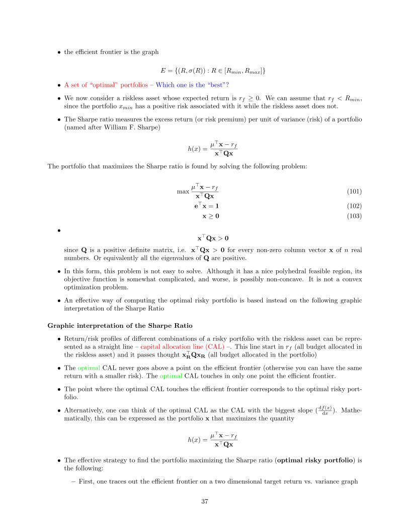
• The Sharpe ratio measures the excess return (or risk premium) per unit of variance (risk) of a portfolio(named after William F. Sharpe)

h(x) =µ>x− rf

x>Qx

The portfolio that maximizes the Sharpe ratio is found by solving the following problem:

maxµ>x− rf

x>Qx(101)

e>x = 1 (102)

x ≥ 0 (103)

•x>Qx > 0

since Q is a positive definite matrix, i.e. x>Qx > 0 for every non-zero column vector x of n realnumbers. Or equivalently all the eigenvalues of Q are positive.

• In this form, this problem is not easy to solve. Although it has a nice polyhedral feasible region, itsobjective function is somewhat complicated, and worse, is possibly non-concave. It is not a convexoptimization problem.

• An effective way of computing the optimal risky portfolio is based instead on the following graphicinterpretation of the Sharpe Ratio

Graphic interpretation of the Sharpe Ratio

• Return/risk profiles of different combinations of a risky portfolio with the riskless asset can be repre-sented as a straight line – capital allocation line (CAL) –. This line start in rf (all budget allocated inthe riskless asset) and it passes thought x>RQxR (all budget allocated in the portfolio)

• The optimal CAL never goes above a point on the efficient frontier (otherwise you can have the samereturn with a smaller risk). The optimal CAL touches in only one point the efficient frontier.

• The point where the optimal CAL touches the efficient frontier corresponds to the optimal risky port-folio.

• Alternatively, one can think of the optimal CAL as the CAL with the biggest slope (df(x)dx ). Mathe-

matically, this can be expressed as the portfolio x that maximizes the quantity

h(x) =µ>x− rf

x>Qx

• The effective strategy to find the portfolio maximizing the Sharpe ratio (optimal risky portfolio) isthe following:

– First, one traces out the efficient frontier on a two dimensional target return vs. variance graph

37

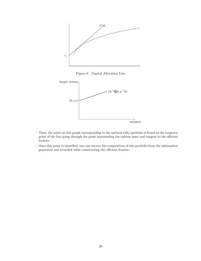
Figure 8: Capital Allocation Line

variance

target return

(0, rf )

(x>Qx, µ>x)

– Then, the point on this graph corresponding to the optimal risky portfolio is found as the tangencypoint of the line going through the point representing the riskless asset and tangent to the efficientfrontier.

– Once this point is identified, one can recover the composition of this portfolio from the informationgenerated and recorded while constructing the efficient frontier.

38

5 Value-at-Risk and Conditional Value-at-Risk

• Financial activities involve risk

• Financial and other institutions must manage risk using sophisticated mathematical techniques

• necessity of quantitative risk measures that adequately reflect the vulnerabilities of a company

• Value-at-Risk and Conditional Value-at-Risk are widely used measure of risk in finance

• They can be used instead of the variance of a portfolio as in the Markowitz model

• This is acheived through stochastic programming

• The random events are modeled by a large but finite set of scenarios, leading to a linear programmingequivalent of the original stochastic program.

5.1 Value-at-Risk – VaR

Definition – Take a random variable X that represents for example the loss of an investment over a fixedperiod of time (a negative value for X indicates gains). Given a probability level α, α-VaR of the randomvariable X is given by the following relation:

V aRα(X) = min{γ : P (X ≤ γ) ≥ α}VaR: represents the predicted maximum loss with a specified probability level (e.g., 95%) over a certain

period of time (e.g.,one day).

Figure 9: 0.95-VaR on a portfolio loss distribution plot

39

Example of application

• take a generic portfolio

• you know its current market value, at the beginning of the day while it is not known its market valueat the end of the day

• The investment bank that holds this portfolio may declare that its portfolio has a 1-day VaR of 0.1million with a confidence level of 95%

• It means that the bank expects that, with a probability of 95%, the portfolio’s loss will not be less than0.1 million during the day

– This implies that the bank expects that the loss of its portfolio at the end of the day will be morethan 0.1 million, with a probability of 5%

– So the bank expects that 5 times out of 100, the portfolio loss will be greater greater than 0.1million, while below this threshold will be 95 times out of 100

Features:

• VaR is widely used by people in the financial industry and VaR calculators are common features inmost financial software

• VaR can be estimated either parametrically (for example, variance-covariance VaR or delta-gammaVaR) or nonparametrically (for examples, historical simulation VaR or resampled VaR)

• 85% of large banks use historical simulation. The other 15% used Monte Carlo methods

Problems:

• it lacks of sub-additivity

• a sub-additive function f(x1 + x2) ≤ f(x1) + f(x1) ∀x1, x2

• a good Risk measures should instead respect the principle that diversification reduces risk

• When VaR is computed by generating scenarios, it turns out to be a non-smooth and non-convexfunction.

• Therefore, when one tries to optimize VaR computed in this manner, the optimization is difficult (globaloptimization algorithms)

• Another criticism on VaR is that it pays no attention to the magnitude of losses beyond the VaR value.

Example:

• Consider two independent and identical investment opportunities:

– 1 of gain with probability 96%

– 2 of loss with probability 4%

• Then, 0.95-VaR for both investments are -1.

• Now consider the sum of these two investment opportunities. Because of independence, this sum hasthe following loss distribution:

– 4 of loss with probability 1.6% (0.04 ∗ 0.04)

– 1 of loss with probability 7.68% (2 ∗ 0.96 ∗ 0.04)

– 2 of gain with probability 92.16% (0.96 ∗ 0.96)

• Therefore, the 0.95-VaR of the sum of the two investments is 1, which exceeds −2, the sum of the0.95-VaR values for individual investments (lacks of sub-additivity).

40

Example of calculation

• consider the following losses of a portfolio over a time window of 20 days

day loss day loss day loss day loss1 10 6 -30 11 20 16 -52 20 7 -40 12 15 17 -103 10 8 10 13 -5 18 104 15 9 15 14 -10 19 155 -30 10 10 15 -10 20 10

• we can now compute and plot the portfolio loss distribution and cumulative loss distribution

loss probability cumulative-40 5.00 100.00-30 10.00 95.00-10 15.00 85.00-5 10.00 70.0010 30.00 60.0015 20.00 30.0020 10.00 10.00

Figure 10: portfolio loss distributionFigure 11: portfolio cumulative loss distri-bution

• the 0.95-VaR is the first point for which the cumulative exceeds 100-95 = 20

• the 0.70-VaR is the first point for which the cumulative exceeds 100-70 = 15

5.2 VaR – with continuous and discrete probability distribution

• We consider a portfolio of assets with random returns

• We denote the portfolio choice vector with x and the random events by the vector y

• Let f (x, y) denote the loss function when we choose the portfolio x from a set X of feasible portfoliosand y is the realization of the random events

• We assume that the random vector y has a probability density function denoted by p(y)

For a fixed decision vector x, we compute the cumulative distribution function of the loss associatedwith that vector x:

41

Continuous probability distribution:

Ψ(x, y) =

∫f(x,y)<γ

p(y) dy

Discrete probability distributions:

Ψ(x, y) =∑

j:f(x,yj)<γ

pj

Then, for a given confidence level α, the α-VaR associated with portfolio x is given as:

V aRα(x) = min{γ ∈ R : Ψ(x, y) ≥ α}

5.3 Conditional Value-at-Risk – CVaR

We define the α-CVaR associated with portfolio x as:

CV aRα(x) =1

1− α

∫f(x,y)≥V aRα(x)

f(x, y)p(y) dy

For a discrete probability distribution (where event yj occurs with probability pj , for j = (1, . . . , n), theabove definition of CVaR becomes:

CV aRα(x) =1

1− α∑

j:f(x,yj)≥V aRα(x)

pjf(x, yj)

Features:

• CVaR of a portfolio is always at least as big as its VaR

• Consequently, portfolios with small CVaR also have small VaR

• However, in general minimizing CVaR and VaR are not equivalent

Example:

• Suppose we are given the loss function f (x, y) for a given decision x as:

• f (x, y) = -yj where yj = 75 - j with probability 1% for j = 0, . . . , 99

• We would like to determine the maximum loss incurred with 95% probability

• This is the Value-at-Risk VaRα (x) for α = 95%

• We have VaR95% (x) = 20 since the loss is less than 20 with probability 95%

• To compute the Conditional Value-at-Risk, we use the above formula:

• CVaR95% (x) =1

0.05(20 + 21 + 22 + 23 + 24) × 1% = 22

42

6 Asset Pricing and Arbitrage

6.1 Pricing and Hedging of Options

We first start with a description of some of the well-known financial options.

European call option: is a contract with the following conditions

• At a prescribed time in the future, known as the expiration date, the holder of the option has the right,but not the obligation to purchase a prescribed asset, known as the underlying, for a prescribed amount,known as the strike price or exercise price.

European put option: is similar, except that it confers the right to sell the underlying asset.

American option: is like a European option, but it can be exercised anytime before the expiration date.

In order to define the price of the option we consider no-arbitrage opportunities:

Definition An arbitrage is a trading strategy:

• that has a positive initial cash flow and has no risk of a loss later (type A)

• that requires no initial cash input, has no risk of a loss, and a positive probability of making profits inthe future (type B).

How can we determine the price of the options?

We start with an example and then we formalize the problem.

• To find the fair value of an option, we need to solve a pricing problem.

• Option pricing problems are often solved using the following strategy:

– We try to determine a portfolio of assets with known prices which, if updated properly throughtime, will produce the same payoff (value) as the option.

– Here a portfolio is the portfolio resulting from a decision of buying or selling stocks and/or sellingor borrowing money

– Since the portfolio and the option will have the same eventual payoffs, we conclude that they musthave the same value today (otherwise, there is arbitrage) and we can therefore obtain the price ofthe option.

– A portfolio of other assets that produces the same payoff as a given financial instrument is calleda replicating portfolio (or a hedge).

– Finding the right portfolio, of course, is not always easy and leads to a replication (or hedging)problem.

Let us consider a simple example to illustrate these ideas:

• We know that one share of stock α is currently valued at e40

• Assume that the value of α will either double or halve with equal probabilities (random values):

• Today, we purchase a European call option to buy one share of stock α for e50 a month from today.What is the fair price of this option?

43

Assumptions

• we can borrow or lend money with no interest between today and next month

• we can buy or sell any amount of the α stock without any commissions

• assume that α will not pay any dividends within the next month.

To solve the option pricing problem, we consider the following hedging problem:

• Can we form a portfolio of the underlying stock (bought or sold) and cash (borrowed or lent) today,such that the payoff of the portfolio at the expiration date of the option will match the payoff of theoption?

• Note that the option payoff will be e30 if the price of the stock goes up and e0 if it goes down.

• Assume this portfolio has ∆ shares of α and B cash.

This portfolio would be worth 40∆+B today. Next month, payoffs for this portfolio will be:

Let us choose ∆ and B such that:80∆ +B = 30

20∆ +B = 0

so that the portfolio replicates the payoff of the option at the expiration date.

• This gives ∆ = 12 and B = -10, which is the hedge we were looking for.

• This portfolio is worth P0 = 40∆ + B =e10 today, therefore, the fair price of the option must also bee10.

6.2 Replication Problem

In this Section we generalize the example of the previous paragraph.

• Let S0 be the current price of the underlying security

• Assume that there are two possible outcomes at the end of the period:

Su1 = S0 · u

andSd1 = S0 · d

(Assume u > d.)

44

• We also assume that there is a fixed interest paid on cash borrowed or lent at rate r for the givenperiod.

R = 1 + r

.

• We consider a derivative security which has payoffs of Cu1 and Cd1 in the up and down states respectively

• The replication problem considers a portfolio of ∆ shares of the underlying and B cash.

• For what values of ∆ and B does this portfolio have the same payoffs at the expiration date as thederivative security?

• We need to solve the following system of 2 equations and 2 variables (∆ and B):

∆ · S0 · u+B ·R = Cu1

∆ · S0 · d+B ·R = Cd1

• This portfolio is worth S0 ·∆ +B today, which corresponds to the fair price of the option as well:

C0 =Cu1 − Cd1u− d

+u · Cd1 − d · Cu1R(u− d)

=1

R

[R− du− d

Cu1 +u−Ru− d

Cd1

]• In the same way we can compute the hedge

∆ =Cu1 ·R− Cd1 ·R

S0 · u ·R− S0 · d ·R

B =S0 · u · Cd1 − S0 · d · Cu1S0 · u ·R− S0 · d ·R

Risk-Neutral Probabilities

Let us define:

pu =R− du− d

and

pd =u−Ru− d

• Note that we must have d < R < u to avoid arbitrage opportunities

• An immediate consequence of this observation is that both pu > 0 and pd > 0

• Noting also that pu + pd = 1 one can interpret pu and pd as probabilities

45

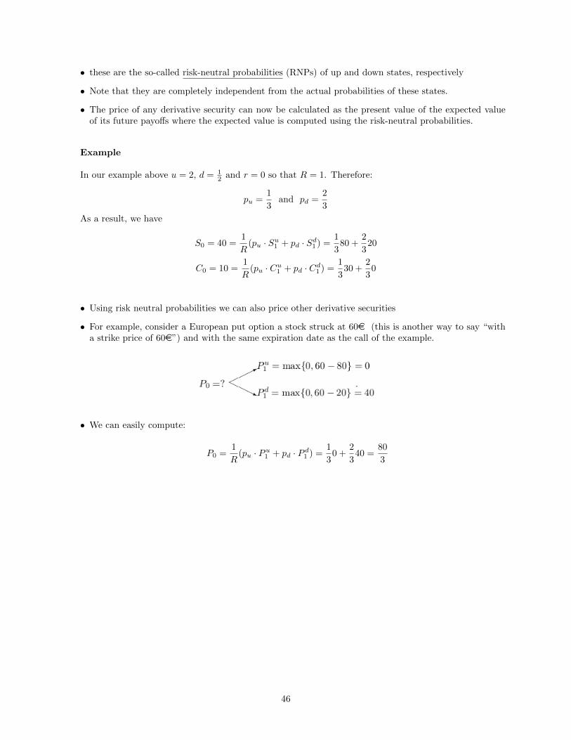
• these are the so-called risk-neutral probabilities (RNPs) of up and down states, respectively

• Note that they are completely independent from the actual probabilities of these states.

• The price of any derivative security can now be calculated as the present value of the expected valueof its future payoffs where the expected value is computed using the risk-neutral probabilities.

Example

In our example above u = 2, d = 12 and r = 0 so that R = 1. Therefore:

pu =1

3and pd =

2

3

As a result, we have

S0 = 40 =1

R(pu · Su1 + pd · Sd1 ) =

1

380 +

2

320

C0 = 10 =1

R(pu · Cu1 + pd · Cd1 ) =

1

330 +

2

30

• Using risk neutral probabilities we can also price other derivative securities

• For example, consider a European put option a stock struck at 60e (this is another way to say “witha strike price of 60e”) and with the same expiration date as the call of the example.

• We can easily compute:

P0 =1

R(pu · Pu1 + pd · P d1 ) =

1

30 +

2

340 =

80

3

46