optical control and quantum information processing with
TRANSCRIPT

University of New MexicoUNM Digital Repository
Physics & Astronomy ETDs Electronic Theses and Dissertations
2-9-2010
Optical control and quantum informationprocessing with ultracold alkaline-earth-like atomsIris Evelyn Nicole Reichenbach
Follow this and additional works at: https://digitalrepository.unm.edu/phyc_etds
This Dissertation is brought to you for free and open access by the Electronic Theses and Dissertations at UNM Digital Repository. It has beenaccepted for inclusion in Physics & Astronomy ETDs by an authorized administrator of UNM Digital Repository. For more information, please [email protected].
Recommended CitationReichenbach, Iris Evelyn Nicole. "Optical control and quantum information processing with ultracold alkaline-earth-like atoms."(2010). https://digitalrepository.unm.edu/phyc_etds/57


Optical Control and QuantumInformation Processing with Ultracold
Alkaline-Earth-like Atoms
by
Iris Reichenbach
Vordiplom, Julius Maximilians Universitat Wurzburg, 2002
M.S., Physics, University of New Mexico, 2005
DISSERTATION
Submitted in Partial Fulfillment of the
Requirements for the Degree of
Doctor of Philosophy
Physics
The University of New Mexico
Albuquerque, New Mexico
December, 2009
iii
c©2009, Iris Reichenbach

iv
Dedication
To Birk

v
Acknowledgments
First and foremost, many thanks to my advisor Ivan Deutsch, who introduced me tothe fascinating field of quantum optics. His enthusiasm and support has helped meto stay motivated and has helped me to develop the skills and confidence needed tobe a scientist.
My thanks also go to Paul Julienne and Eite Tiesinga for teaching me much aboutcollisional and atomic physics.
I also want to thank Rene Stock who has taught me quite a bit of scatteringtheory and who, together with Shohini Ghose always had valuable advise for me.Furthermore, many thanks to the whole Information Physics Group for many inter-esting discussions over the years, some of which were actually about physics. I mademany friends on my way and I want to thank all of you. Most importantly, I want tothank my husband Birk for all his support. Thank you for always being there whenI need you.

Optical Control and QuantumInformation Processing with Ultracold
Alkaline-Earth-like Atoms
by
Iris Reichenbach
ABSTRACT OF DISSERTATION
Submitted in Partial Fulfillment of the
Requirements for the Degree of
Doctor of Philosophy
Physics
The University of New Mexico
Albuquerque, New Mexico
December, 2009

vii
Optical Control and QuantumInformation Processing with Ultracold
Alkaline-Earth-like Atoms
by
Iris Reichenbach
Vordiplom, Julius Maximilians Universitat Wurzburg, 2002
M.S., Physics, University of New Mexico, 2005
PhD, Physics, University of New Mexico, 2009
Abstract
Ultracold neutral atoms in optical lattices are rich systems for the investigation
of many-body physics as well as for the implementation of quantum information
processing. While traditionally alkali atoms were used for this research, in recent
years alkaline-earth-like atoms have attracted considerable interest. This is due to
their more complex but tractable internal structure and easily accessible transitions.
Furthermore, alkaline-earth-like atoms have extremely narrow 1S → 3P intercombi-
nation transitions, which lend themselves for the implementation of next generation
atomic clocks.
In this dissertation, I show that exquisite control of alkaline-earth-like atoms can
be reached with optical methods, and elucidate ways to use this controllability to
further different aspects of research, mainly quantum information processing. Ad-

viii
ditionally, the control of alkaline-earth-like atoms is very interesting in many-body
physics and the improvement of atomic clocks.
Since heating usually degrades the performance of quantum gates, recooling of
qubits is a necessity for the implementation of large scale quantum computers. Laser
cooling has advantages over the usually used sympathetic cooling, given that it re-
quires no additional atoms, which have to be controlled separately. However, for
qubits stored in hyperfine states, as usually done in alkali atoms, laser cooling leads
to optical pumping and therefore to loss of coherence. On the other hand, in the
ground state, the nuclear spin of alkaline-earth-like atoms is decoupled from the elec-
tronic degrees of freedom. As I show in this dissertation, this allows for the storage of
quantum information in the nuclear spin and laser cooling on the electronic degrees
of freedom. The recooling protocol suggested here consists of two steps: resolved
sideband cooling on the extremely narrow 1S0 → 3P0 clock transition and subse-
quent quenching on the much shorter lived 1P1 state. A magnetic field is used to
overcome the hyperfine interaction in this excited state and thus ensures decoupling
of the nuclear spin degrees of freedom during the quenching. The application of this
magnetic field also allows for photon scattering on the 1P1 state, while preserving
the nuclear spin, e. g. for electronic qubit detection.
The manipulation of the scattering properties of neutral atoms is an important
aspect of quantum control. In contrast to alkali atoms, whose broad linewidths cause
large losses, this can be done with purely optical methods via the implementation
of an optical Feshbach resonance for alkaline-earth-like atoms. Here, the scatter-
ing length resulting from the application of an optical Feshbach resonance on the
1S0 → 3P1 intercombination line, including hyperfine interaction and rotation is cal-
culated for 171Yb. Due to their different parities, the p-wave scattering length can
be controlled independently from the s-wave scattering length, thus allowing for un-
precedented control over the scattering properties of neutral atoms. Furthermore, I
also show how optical Feshbach resonances in alkaline-earth-like atoms can be used
ix
together with the underlying quantum symmetry to implement collisional gates be-
tween nuclear-spin qubits over comparatively long ranges.

x
Contents
List of Figures xiii
List of Tables xv
1 Introduction 1
1.1 Cold Atoms in Optical Lattices . . . . . . . . . . . . . . . . . . . . . 4
1.2 Quantum Information Processing . . . . . . . . . . . . . . . . . . . . 6
1.3 Alkaline-Earth-like Atoms . . . . . . . . . . . . . . . . . . . . . . . . 8
1.4 Overview of Thesis . . . . . . . . . . . . . . . . . . . . . . . . . . . . 11
2 Theoretical Background 13
2.1 Scattering Theory . . . . . . . . . . . . . . . . . . . . . . . . . . . . . 14
2.2 Controlled Collisions in Quantum Information Processing . . . . . . . 19
2.3 Molecular States . . . . . . . . . . . . . . . . . . . . . . . . . . . . . 22
2.3.1 Hund’s Cases . . . . . . . . . . . . . . . . . . . . . . . . . . . 25
2.3.2 Including Nuclear Spin and Hyperfine Interaction . . . . . . . 27

Contents xi
2.3.3 Molecular States for Nuclear Rotation . . . . . . . . . . . . . 28
2.3.4 Transformation between Basis States . . . . . . . . . . . . . . 31
3 Cooling Atomic Vibration without Decohering Qubits 37
3.1 Theoretical Background . . . . . . . . . . . . . . . . . . . . . . . . . 37
3.1.1 Resolved Sideband Cooling . . . . . . . . . . . . . . . . . . . . 39
3.2 Description of the Proposed Cooling Scheme . . . . . . . . . . . . . . 44
3.2.1 Resolved Sideband Cooling on the Clock Transition . . . . . . 45
3.2.2 Quenching of a Metastable State via a Rapidly Decaying State 47
3.2.3 Decoupling the Nuclear Spin from the Electronic Degrees of
Freedom in the Quenching Process . . . . . . . . . . . . . . . 51
3.3 Results . . . . . . . . . . . . . . . . . . . . . . . . . . . . . . . . . . . 53
3.4 Flourescence while Preserving Nuclear Spin Coherences . . . . . . . . 55
4 Optical Feshbach Resonances for 171Yb 66
4.1 Background . . . . . . . . . . . . . . . . . . . . . . . . . . . . . . . . 66
4.1.1 Feshbach resonances in controlling atom-atom interactions . . 67
4.1.2 Magnetic vs. Optical Feshbach resonances . . . . . . . . . . . 68
4.1.3 Theory of optical Feshbach resonances . . . . . . . . . . . . . 70
4.2 Calculation . . . . . . . . . . . . . . . . . . . . . . . . . . . . . . . . 72
4.2.1 Ground States . . . . . . . . . . . . . . . . . . . . . . . . . . . 72
4.2.2 Excited States . . . . . . . . . . . . . . . . . . . . . . . . . . . 74

Contents xii
4.2.3 Channel Bases . . . . . . . . . . . . . . . . . . . . . . . . . . . 76
4.3 Results . . . . . . . . . . . . . . . . . . . . . . . . . . . . . . . . . . . 79
4.3.1 Selective Change of a for P-waves and S-waves . . . . . . . . . 79
4.3.2 Purely Long-Range States . . . . . . . . . . . . . . . . . . . . 83
4.3.3 Excited-State Spectrum . . . . . . . . . . . . . . . . . . . . . 86
4.3.4 Scattering Length . . . . . . . . . . . . . . . . . . . . . . . . . 90
4.4 Application to QIP . . . . . . . . . . . . . . . . . . . . . . . . . . . . 93
4.5 Conclusions . . . . . . . . . . . . . . . . . . . . . . . . . . . . . . . . 96
5 Summary and Outlook 101
Appendices 107
A Programs 108
A.1 Calculation of the Breit-Rabi spectrum . . . . . . . . . . . . . . . . . 108
A.2 Inclusion of the quadrupole part for Sr . . . . . . . . . . . . . . . . . 117
A.3 Calculation of the multichannel Hamiltonian . . . . . . . . . . . . . . 124
A.4 Determination of the optically induced scattering length . . . . . . . 138
References 149

xiii
List of Figures
2.1 Implementation of a state dependent controlled collision. . . . . . . 20
2.2 Optical lattice for alkaline-earth-like atoms . . . . . . . . . . . . . . 33
2.3 Schematics of Hund’s case c) coupling . . . . . . . . . . . . . . . . . 34
2.4 Schematics of Hund’s case e) coupling . . . . . . . . . . . . . . . . . 35
2.5 Schematics of Hund’s case a) coupling . . . . . . . . . . . . . . . . . 36
2.6 The classical motion of a symmetric top. . . . . . . . . . . . . . . . 36
3.1 Schematics of resolved sideband cooling. . . . . . . . . . . . . . . . . 60
3.2 Schematic cooling and readout level-diagram for 171Yb. . . . . . . . 61
3.3 Zeeman diagram of the 1P1 manifold. . . . . . . . . . . . . . . . . . 62
3.4 Field dependent expansion coefficients cq for the mf state of 171Yb . 63
3.5 Fidelity for transfer of coherence for the proposed cooling scheme. . 64
3.6 Scattering rates for alternative cooling scheme. . . . . . . . . . . . . 65
4.1 Schematics of a Feshbach resonance. . . . . . . . . . . . . . . . . . . 67
4.2 S-wave ground state wave functions . . . . . . . . . . . . . . . . . . 72

List of Figures xiv
4.3 The adiabatic potentials for s-wave collisions. . . . . . . . . . . . . . 80
4.4 The adiabatic potentials for p-wave collisions. . . . . . . . . . . . . . 81
4.5 Adiabatic purely long-range potentials for s-waves . . . . . . . . . . 83
4.6 Adiabatic purely long-range potentials for p-waves . . . . . . . . . . 84
4.7 Purely-long range states for p-waves . . . . . . . . . . . . . . . . . . 85
4.8 S-wave spectrum for 171Yb . . . . . . . . . . . . . . . . . . . . . . . 87
4.9 P-wave spectrum for 171Yb . . . . . . . . . . . . . . . . . . . . . . . 88
4.10 Multi-channel states for s-waves . . . . . . . . . . . . . . . . . . . . 91
4.11 Scattering length for s-wave optical Feshbach resonances . . . . . . . 92
4.12 The optical Feshbach resonance leading to nuclear spin exchange. . . 99
4.13 The fidelity of a√SWAP gate . . . . . . . . . . . . . . . . . . . . . 100

xv
List of Tables
1.1 The stable isotopes of Yb and Sr . . . . . . . . . . . . . . . . . . . . 9
1.2 List of publications . . . . . . . . . . . . . . . . . . . . . . . . . . . 12
4.1 The |ε〉 basis for s-wave states . . . . . . . . . . . . . . . . . . . . . 81
4.2 The |ε〉 basis for p-wave states . . . . . . . . . . . . . . . . . . . . . 82
4.3 Excited molecular bound states and resonance properties for s-waves 89
4.4 P-wave accessible excited molecular bound states. . . . . . . . . . . 98

1
Chapter 1
Introduction
Over the last decades, several different areas of research have driven a renewal in
atomic, molecular and optical (AMO) physics. The quest for ever more accurate
time standards caused investigations into improving the coherences of atoms for the
use in atomic clocks, the advent of laser cooling and trapping made exquisite control
over the states of atoms possible, and the prediction of the advantages of quantum
information processing over classical information processing have spurred even more
research on the coherent control of quantum systems. Due to the improvements in
these interdependent areas of basic research, we have now excellent control over the
positions, internal states and interactions of single atoms as well as of many-body
states.
While measurement of time was important for practical purposes as well as for
social and cultural reasons throughout human history, its relevance and the required
accuracy has increased dramatically in the last centuries. With the advent of the
industrial revolution, traveling times decreased and the communication over wide
distances became possible, thus requiring a reliable standard of time. But even then,
as during all of human history, time was measured with the help of astronomical
observations. However, in the last century this way of measuring time was neither

Chapter 1. Introduction 2
practical nor accurate enough, given the further acceleration of our society and the
technical progress that required more and more accurate timekeeping. This lead to
the development of atomic clocks, in which the natural oscillation frequency of atoms
is used to measure time, which has several advantages over earlier methods. Since
all atoms of a given isotope have the exact same oscillation frequency, atomic clocks
are a much more universal time standard then other measurements. Furthermore,
astronomical observations generally have a low frequency, requiring the division of
one oscillation period, while the much higher frequency of atomic transitions merely
requires counting of oscillations, which is much easier. These advantages lead to the
adoption of the oscillation frequency of Cesium as international time standard in
1967, as well as to the redefinition of the meter in terms of the so defined second and
the speed of light, c. Modern Cesium fountain clocks have a fractional instability,
that is the error of the clock frequency divided by the frequency of the clock, of
σ = 1 × 10⁻¹⁴T−1/2 [1]. Generally, the fractional instability of an atomic clock is
given by
σ =∆ν
ν
C
2π√NT
, (1.1)
where C is a constant of order unity, T is the interrogation time, N is the number of
interrogated atoms, and ∆ν is the linewidth of the clock transition with frequency
ν [2, 1]. This shows that the fractional instability can be decreased by interrogating
more atoms or by choosing a transition with a longer lifetime or higher frequency.
To take advantage of an increase of the number of atoms N or the interrogation
time T , however, these atoms have to be coherent. Thus, the system has to be very
well isolated from the environment, e.g stray magnetic or electric fields as well as
electromagnetic radiation have to be suppressed. Furthermore, to avoid effects due
to the motion of the atoms, they have to be cooled to very low temperatures and/or
tightly confined to traps.
During the 1980’s, laser cooling and trapping of atoms was developed, which
is continuing to have wide implications for several other fields of physics. Due to

Chapter 1. Introduction 3
the development of optical molasses, that is counterpropagating laser beams that
exert a drag on atoms, by Chu and Hollberg in 1985, neutral atoms could be cooled
to very low temperatures for the first time. A closely related technique, Sisyphus
cooling, which was accidentally discovered in molasses experiments and theoretically
explained in 1989 by Dalibard and Cohen-Tannoudji, makes it possible to cool neutral
atoms to temperatures below the Doppler limit, which was before considered to be
the absolute limit of laser cooling. Furthermore, the development of magneto-optical
traps by Chu in 1987 made it first possible to trap these ultracold atoms with laser
light. Additionally, a consequence of optical molasses and Sisyphus cooling is the
realization of optical lattices, in which atoms are trapped in a periodic potential
created by standing waves from counterpropagating laser beams, which was first
realized in 1992 by Jessen et al.. An in-depth account of these achievements can be
found in the Nobel lectures by Chu [3], Cohen-Tannoudji [4] and Phillips [5] from
1998, and references therein.
Cold atoms trapped in optical traps show coherences over long times and large
distances, and allow for the control of their interactions, thus furthering atomic
clocks, but also allowing for other basic research, e. g. the exploration quantum
phase transitions and many-body effects. The goal of this thesis is to contribute to
this young and rapidly developing field, by exploring possibilities of enhancing this
control and applying it to the implementation of quantum information processing
(QIP), another rapidly emerging field which harnesses the existence of superpositions
and long range entanglement to process information more rapidly than possible with
purely classical methods, as was shown in 1985 by D. Deutsch [6].
Alkaline-earth atoms are especially well suited for several of these applications,
due to their interesting properties, e.g. the existence of narrow intercombination
transitions. One of these transitions, the so-called clock transition, is particularly
suitable for the use in atomic clocks, due to its narrow linewidth on the order of tens
of mHz, and its oscillation frequency in the optical range. Thus, the quality factor

Chapter 1. Introduction 4
Q = ν/∆ν of this transition is very high, promising a clock with very low fractional
instability, as can be seen from (1.1). For the implementation of this clock, alkaline-
earth atoms are trapped in an optical lattice and the clock transition is interrogated,
allowing for the most accurate clock with neutral atoms to date. Considering the
fact that it is possible to increase the number of atoms trapped in the optical lattice,
this clock has the potential to surpass the accuracy of the most accurate clock to
date, which is based on a single Hg+ ion [7, 8]. Additionally, the absence of hyperfine
interaction in the ground state allows for the storage of qubits in the nuclear spin of
the atoms, rendering the qubits well isolated and causing extremely long coherence
times. Furthermore, as I show in this dissertation, the narrow intercombination lines
provide for excellent control over the two-body interactions that are at the heart of
cold AMO physics, via optical Feshbach resonances. Additionally, I suggest a way of
laser cooling alkaline-earths that enables the preservation of nuclear spin coherences
and thus could prove very useful in the implementation of QIP.
In the following sections I will elucidate some background to AMO physics and
QIP. In the final section of this chapter, I will give an overview over this thesis.
1.1 Cold Atoms in Optical Lattices
Over the last decades, quantum control of cold atoms has been employed in many
different aspects of basic research. One major advancement was the trapping of
atoms in optical lattices [9]. These artificial crystals of single atoms can be used to
investigate the interactions between atoms as well as many-body effects and quantum
phase transitions. Furthermore, there are several proposals for the implementation
of quantum computation and quantum simulation in optical lattices [10, 11, 12, 13].
An optical lattice consists of two counterpropagating laser beams for each spatial
trapping dimension, which form a superposition of standing waves with opposite

Chapter 1. Introduction 5
helicity given by
EL =√
2E0 (cos (kLz + θ/2)ε+ + cos (kLz − θ/2)ε−) , (1.2)
where θ is the angle between the polarizations of the laser beams, E0 is the amplitude
of the electric field of the lasers, kL is the wavenumber of the lasers and z denotes
the direction of the laser beams, here chosen to be along the z-axis. Atoms in such
a standing wave experience a light shift of
U = −1
4E∗L · α · EL, (1.3)
where α is the atomic polarizability. While the atomic polarizability generally con-
sists of a scalar, vector and second rank tensor part, for alkaline-earth-like atoms
which have no hyperfine interaction in the ground state, only the scalar part is rele-
vant. With more complicated laser configurations, it is possible to create much more
complicated and controllable optical lattices, as shown by Sebby-Stradley et al. [14].
This allows for the lattice geometry to be changed such that atoms are moved from
neighboring lattice sites into one double well or single well, where they can inter-
act more strongly. Due to this controllability, optical lattices have proven to be an
useful tool for basic research, in which many studies of scattering theory and phase
transitions have been realized. Noteworthy are, among others, the Mott-insulator to
superfluid transition, in which either the relative phase of the atoms or the number
of atoms per lattice site are well defined, depending on the specific parameters of the
optical lattice [15]. From a condensed matter physics perspective, ultracold atoms
trapped in optical lattices provide an ideal system for studying tight-binding models
such as the Hubbard model [9, 16, 17]. There are also interesting proposals for new
applications such as quantum simulators and universal quantum computers using
ultracold neutral atoms trapped in optical lattices [18].

Chapter 1. Introduction 6
1.2 Quantum Information Processing
Quantum computing utilizes long range entanglement and coherences to speed up
some calculations compared to classical computers. To date, there are several known
quantum algorithms whose large scale implementation would significantly change
the world of computing, e.g. Grover’s algorithm, which allows to search unordered
datasets and Shor’s algorithm, which allows to factor big numbers exponentially
faster then any classical algorithm [6]. The latter is particularly important, since
most of todays encryption is based on the fact that it is very hard to factor big num-
bers. However, the growing field of quantum cryptography, in which eavesdropping
leads to detectable decoherence, offers the first and to date only encryption system
that is safe on purely physical grounds. Another very important application of this
is the simulation of quantum systems, which is hard classically, since the complexity
of quantum systems scales exponentially in the size of the system, as opposed to the
linear scaling in classical systems [6].
However, being based on quantum mechanical effects, quantum computing has
several requirements that are much harder to fulfill than the requirements for classical
information processing [6]. The first requirement for QIP is the existence of robust
qubits, which will not decohere too quickly, necessitating a system that interacts only
weakly with the environment. At the same time, we need the ability to subject the
qubits to quantum gates, which have to be fast relative to the coherence times, to
allow for many operations during the lifetime of the qubits. This requires the qubits
to interact strongly with each other and with some external control field. These
conditions are somewhat contradicory, since often the same interaction that allows
for manipulation of qubits also causes decoherence. Additional requirements are the
possibility of initialization of the qubits in a well-defined state, for which there are
promising avenues for neutral atoms in optical lattices, e.g. using the Mott-insulator
to superfluid transition [19] as well as readout of the qubits after the computation.

Chapter 1. Introduction 7
The latter also requires the ability to suddenly turn on a strong interaction with the
environment. One possible realization for this is to use a fluorescence interaction on
a strong line selectively on different basis states of the qubit for which I will also
suggest an implementation.
Many different physical systems have been suggested for the implementation of
quantum information [6], e.g. nuclear spins in NMR systems, trapped ions, super-
conducting qubits, solid state systems such as quantum dots as well as photons in
cavities. As mentioned before, there are also several proposals for the use of neutral
atoms in optical lattices [10, 11, 12, 13]. As of yet, there are no systems that accord
truly scalable QIP, even though progress has been made in all of these systems.
In this thesis I will show that neutral alkaline-earth atoms in optical lattices as
carriers of quantum information are a very promising system that allows to circum-
vent the earlier mentioned contradiction. The reason for this is that the neutral
atoms in an optical lattice are well isolated from each other and from their environ-
ment. However, the rich possibilities of control and deformation of optical lattices
and the possibility to significantly increase the interaction strength between neutral
atoms due to Feshbach resonances, make strong interactions between selected atoms
possible. Furthermore, such arrays of optical traps provide a scalable platform for
storing many qubits, with parallel operations, applicable to the generation of clus-
ter states for one-way quantum computing [20], quantum-cellular automata [11, 20],
or more general quantum circuit operations [10], and fault-tolerance via topological
encoding [21].
Traditionally, the research on neutral atoms for QIP and quantum control has
focused on alkali atoms, owing to their good controllability after decades of research
based on this system. However, recently group-II and group-II-like atoms like Yb
have emerged as good candidates for the implementation of quantum information
processing [13, 22]. This is due to their convenient optical transitions, and rich
but tractable internal structure as well as the relative ease with which they can be
Chapter 1. Introduction 8
trapped and cooled. Furthermore, the distinguishing feature of alkaline-earth-like
atoms is the fact that in the ground state the electron spins couple together to give
an angular momentum of zero, causing the nuclear spin to be decoupled from the
electronic degrees of freedom. As will be seen in this thesis, this allows for the storage
of the quantum information in the nuclear spin, which in turn affords not only the
optical recooling of qubits between and during the gates, but also very long coherence
times in spite of strong interactions and therefore fast gates and our ability to control
them with the mature tools of NMR [23].
The latter can be enhanced by the application of optical Feshbach resonances,
which are possible in alkaline-earth-like atoms, due to their very narrow intercombi-
nation transitions. These optical Feshbach resonances have the potential to enhance
basic research by adding another knob to the control of ultracold atoms, given their
faster controllability and and independence of hyperfine states compared to their
magnetic equivalent.
1.3 Alkaline-Earth-like Atoms
Alkaline-earth atoms, that is, atoms in the second column of the periodic table, have
two valence electrons. This is also true for Yb, the element 70, which is a rare-earth
element with the ground state configuration [Xe]4f 146s2. Since 14 is the maximum
number of electrons in the f shell, this shell is closed and the 6s2 electrons are the
valence electrons interacting with the environment, causing Yb to behave in the same
way as alkaline-earth atoms. Therefore, I will use the term alkaline-earth-like atoms
to refer to Yb and alkaline-earth atoms. Most of the work in this thesis has been
done on the example of Yb and Sr, however, in principle it is more general than
that and also applicable to other alkaline-earth-like atoms. In the ground state, the
spins of the two electrons couple together to give zero total electron spin. Since,
in the ground state, the electronic orbital angular momentum is also zero, the total

Chapter 1. Introduction 9
angular momentum of the electrons also has to be zero and the ground state is 1S0,
and the only relevant spin is the nuclear spin. For the bosonic isotopes of Sr and
Yb, the nuclear spin is also zero, resulting in a completely spinless ground state.
However, both Sr and Yb have a multitude of different stable isotopes, with different
nuclear spins, including both fermions with finite nuclear spin and bosons. The stable
isotopes of Yb and Sr are given in table 1.1.
atomic nr. (Yb) i168 0170 0171 1/2172 0173 3/2174 0176 0
atomic nr. (Sr) i84 086 087 9/288 0
Table 1.1: The stable isotopes of Yb and Sr, i denotes the nuclear spin. For thepurposes of this thesis, the fermionic isotopes are relevant, specifically 171Yb and87Sr.
In the excited states, the electron spins can be coupled together to give a finite
electron spin of s = s1 + s2 = 1, giving rise to triplet excited states, as for example
the (nsnp) 3Pj state, which is the lowest excited state, with n = 5 for Sr and n = 6
for Yb. Due to selection rules, direct coupling between singlet and triplet states is
forbidden. However, these states are not pure spin-orbit LS coupling, causing an
admixture of the higherlying (nsnp) 1P1 state, such that [7, 24]
|3P2〉 = |3P 02 〉 (1.4a)
|3P1〉 = α|3P 01 〉+ β|1P 0
1 〉 (1.4b)
|3P0〉 = |3P 00 〉 (1.4c)
|1P1〉 = −β|3P 01 〉+ α|1P 0
1 〉, (1.4d)
where the states with the superscript 0 denote states with pure spin-orbit coupling.
Chapter 1. Introduction 10
Hence, the intercombination transition 1S0 → 3P1 is weakly allowed,
〈3P0|d · ε|3P1〉 = α〈3P 00 |d · ε|3P 0
1 〉+ β〈3P 00 |d · ε|3P 0
1 〉. (1.5)
where the first part on the right side is zero. This results in a line width of 182 kHz
for 171Yb and 80 kHz for 87Sr. The transition from the ground state to the 3P0 and
3P2 is additionally forbidden, since the selection rules for j require ∆j = 0, 1 and
j = 0 9 j = 0, causing lifetimes on the order of 1000 years for the metastable 3P0
state for the bosonic isotopes. For fermionic alkaline-earth-like elements, which have
half-integer nuclear spin, however, the hyperfine interaction couples the states with
equal total spin f and thus causes an additional admixture of the |3P1〉, |1P1〉 and
|3P2〉 states to the |3P0〉 state, resulting in
|3P0〉 = |3P 00 〉+ α0|3P1〉+ β0|1P1〉+ γ0|3P 0
2 〉. (1.6)
This reduces the lifetime of the clock transition, 1S0 → 3P0 to about 100 s for 87Sr and
to 10 s for 171Yb with its larger hyperfine interaction [24]. It is also possible to induce
a similar coupling with the application of a magnetic field or an additional laser and to
thus reduce the lifetime of the clock state of the bosonic elements [25, 26]. These long
lifetimes, in combination with easily accessible transition frequencies, have caused
the alkaline-earth-like elements to emerge in different areas of quantum control, most
notably in the implementation of atomic clocks, as pointed out in Section 1.
Due to the fact that their only spin is the nuclear spin, the Hamiltonian for the
|3P0〉 and the |1S0〉 state in the presence of a weak magnetic field B is given by
HZ = gSµB s ·B/h+ gLµB l ·B/h− gIµB i ·B/h (1.7)
Where µB is the Bohr magneton, gS ' 2 and gL = 1 are the g-factors for electron spin
and electron orbital angular momentum respectively, and gI is the nuclear g-factor.
In the absence of the small admixture of the |3P1〉 state to the |3P0〉 state, Eq. (1.7)
would reduce to −gIµB i ·B/h and the nuclear g-factor gI of the |3P0〉 state would be
exactly the same as for the |1S0〉 ground state. However, the coupling between the

Chapter 1. Introduction 11
two states causes a small admixture of the electron g-factor to the nuclear g-factor.
This leads to a differential g-factor δg for the |3P0〉 state compared to the ground
state. For 87Sr, the difference in g-factors between the two states is about 60%. [24].
Furthermore, the quantum number for the Zeeman interaction for a magnetic field
along the z-axis is not pure mi any more, but mf , due to the small admixture of
the other states, causing the Zeeman shift to be δgmfµBB/h. This effect has to be
taken into account for applications in optical clocks as well as for coherent transfer
of population from different nuclear spin states in the ground state to the |3P0〉 state.
On the other hand, together with the extremely narrow linewidth of the |3P0〉 state,
this also allows for controlled excitation of different nuclear spin states independently
from each other, which makes complete control over the nuclear spin submanifold of
these states possible.
1.4 Overview of Thesis
This thesis aims to elucidate different aspects of control of ultracold atoms in opti-
cal lattices, focusing on controlled collisions and optical recooling while preserving
internal coherences. All these aspects could be useful in the application of quan-
tum information and, more generally, in basic research e.g. on many-body states.
In Chapter 2, I will give the theoretical background behind many of the calcula-
tions done in this thesis. Chapter 3 will show the possibility of recooling of neutral
alkaline-earth atoms, while preserving nuclear spin coherences. This makes neutral
alkaline-earth-like atoms with nuclear-spin qubits the only system of neutral atoms
that allows optical recooling of qubits between and during the implementation of
quantum gates, ensuring high fidelity of subsequent gates. Chapter 4 will elaborate
on the possibilities of using optical Feshbach resonances to control alkaline-earth-like
atoms and to speed up quantum gates. Finally, in chapter 5, I will summarize and
provide an outlook to open questions in the field.

Chapter 1. Introduction 12
Several parts of this dissertation have previously been published, as is shown
in Table 1.2. Furthermore, I developed a quasi-Hermitian pseudopotential for the
calculation of higher partial-wave collisions. While the pseudopotential proposed
by R. Stock et al. [27, 28] is not Hermitian, it can still be used to calculate the
eigenenergies of atoms colliding via higher partial waves. However, it does not give
rise to acomplete, orthogonal set wave functions that can be used to expand possible
additional parts of an Hamiltonian. The quasi-Hermitian pseudopotential on the
other hand gives rise to a biorthonormal set of wave functions that can be applied
to this purpose. This research was published in [29], but is not shown here.
Chapter Publication
Chapter 3 I. Reichenbach and I. H. DeutschSideband Cooling while Preserving Coherences in the NuclearSpin State in Group-II-like Atoms,Phys. Rev. Lett. 99, 123001 (2007) [30]
Chapter 4 I. Reichenbach, P. S. Julienne and I. H. DeutschControlling nuclear spin exchange via optical Feshbachresonances in 171Yb,accepted for Phys. Rev. A
– I. Reichenbach, A. Silberfarb, R. Stock and I. H. DeutschQuasi-Hermitian pseudopotential for higher partial wavescatteringPhys. Rev. A 74, 042724 (2006) [29]
Table 1.2: List of publications and the corresponding parts of this dissertation, ifapplicable.

13
Chapter 2
Theoretical Background
In this dissertation I consider the manipulation of ultracold alkaline-earth-like atoms
trapped in optical lattices and their use in the implementation of quantum informa-
tion processing. Here, I will give some of the theoretical background which is the
basis of many of the calculations shown in later chapters.
At the fundamental level, quantum many-body systems are governed by their two-
body interactions. In the case of ultracold neutral atoms, these consist of collisions
determined by the diatomic molecular interaction potential. Therefore, in the first
section of this Chapter, I will give a general overview of scattering theory, which is
necessary to understand the scattering length, a very important parameter which
is manipulated with Feshbach resonances and is at the heart of the control scheme
proposed in Chapter 4.
In Section 2.2, I will show how ultracold collisions of atoms in optical lattices
can be controlled and how these controlled collisions of ultracold atoms can be used
to implement a quantum gate by utilizing the effects of symmetry and the Pauli-
exclusion principle.
In the last section, the molecular basis states used for the calculation of the

Chapter 2. Theoretical Background 14
optical Feshbach resonances in Chapter 4, as well as their transformations, will be
derived.
2.1 Scattering Theory
Scattering theory, which describes the effects of collisions of two or more particles on
their states, is a very important tool in theoretical physics. For this dissertation, it is
the basis for both controlled collisions and Feshbach resonances as used in Chapter
4. For this reason, I will give a short overview of scattering theory, limited to two
colliding particles in the center of mass frame or, equivalently, the scattering of one
particle off a stationary target. For more information, see the textbook by Taylor
[31].
Consider a scattering event that consists of two particles which interact via a
potential V (r) with finite range, colliding at time t = t0. At time t → −∞ the
incoming state |ψin〉 is outside of the range of the scattering potential V (r). However,
at time t0 it has moved into the range of the potential and has become the state
|ψ〉 = Ω+|ψin〉, (2.1)
where Ω+ is the Møller operator that embodies the evolution of the undisturbed
incoming state and
|ψ〉 = Ω−|ψout〉 (2.2)
describes the evolution from time t = t0 to the outgoing state |ψout〉 at time t→∞
that is again outside of the range of the interaction potential, with the corresponding
Møller operator Ω− [31].
Since usually, only the incoming and the outgoing state are known, it is advan-
tageous to cast the problem in terms of the so-called S-matrix, which describes the
Chapter 2. Theoretical Background 15
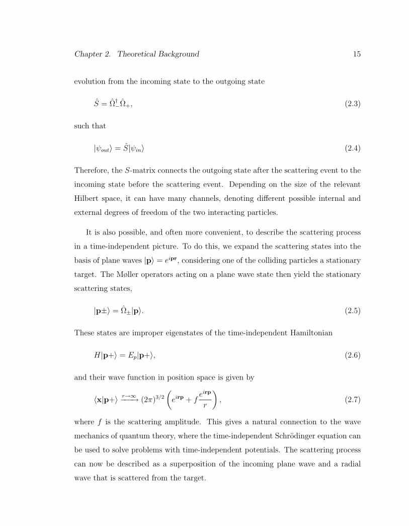
evolution from the incoming state to the outgoing state
S = Ω†−Ω+, (2.3)
such that
|ψout〉 = S|ψin〉 (2.4)
Therefore, the S-matrix connects the outgoing state after the scattering event to the
incoming state before the scattering event. Depending on the size of the relevant
Hilbert space, it can have many channels, denoting different possible internal and
external degrees of freedom of the two interacting particles.
It is also possible, and often more convenient, to describe the scattering process
in a time-independent picture. To do this, we expand the scattering states into the
basis of plane waves |p〉 = eipr, considering one of the colliding particles a stationary
target. The Møller operators acting on a plane wave state then yield the stationary
scattering states,
|p±〉 = Ω±|p〉. (2.5)
These states are improper eigenstates of the time-independent Hamiltonian
H|p+〉 = Ep|p+〉, (2.6)
and their wave function in position space is given by
〈x|p+〉 r→∞−−−→ (2π)3/2
(eirp + f
eirp
r
), (2.7)
where f is the scattering amplitude. This gives a natural connection to the wave
mechanics of quantum theory, where the time-independent Schrodinger equation can
be used to solve problems with time-independent potentials. The scattering process
can now be described as a superposition of the incoming plane wave and a radial
wave that is scattered from the target.

Chapter 2. Theoretical Background 16
In many cases, the Hamiltonian and therefore the S-matrix are invariant under
rotation. In this case, we can define the stationary basis states with energy E, total
angular momentum l and projection of the angular momentum m in terms of the
spherical harmonics and a radial part
|E, l,m〉 = Rl(r)Yml (θ, φ) (2.8)
The S-matrix is diagonal in the |E, l,m〉 basis
〈E ′, l′,m′|S|E, l,m〉 = δ(E ′ − E)δl′lδm′msl(p). (2.9)
Here sl(p) is the S-matrix for a given “partial wave” with well-defined total angular
momentum l. The radial part of the time independent Schrodinger equation (TISE)
becomes[~2
2µ
d2
dr2− l(l + 1)
r2+ V (r)
]Rl(r) = EkRl(r). (2.10)
Ultracold atoms can have a very long deBroglie wavelength, on the order of microns,
whereas the van der Waals interaction for alkali atoms is on the order of 1-10 A[32].
in this case, the expansion in partial waves is very useful, due to the fact that the
kinetic energies are very small compared to the centrifugal barriers l(l + 1)/r2 for
higher l partial waves, which therefore do not interact and can be ignored. In fact,
very often it is sufficient to only take the first few partial waves, namely s and p
waves into account. This is due to the Wigner-threshold law, which states that for
low energies, the phase shift scales as δl(k) ∝ −k2l+1, where k is the deBroglie wave
number for the relative motion. Here δl is the scattering phase shift, which in turn
is given by
sl = ei2δl . (2.11)
For scattering from a short-range, radially symmetric potential, the effect of the
interaction is to phase shift the radial wave function. The stationary scattering
solutions are then given by
ψl,p(r)r→∞−−−→ jl(pr) + pfl(p)e
i(pr−lπ/2), (2.12)

Chapter 2. Theoretical Background 17
where jl is a spherical Bessel function and fl is the scattering amplitude for partial
wave l, which can be written as
fl(p) =1
peiδl sin (δl). (2.13)
The scattering phase shift δl denotes the amount by which a free stationary scattering
state is phase shifted due to the interaction process, as can be seen by inserting Eq.
(2.12) into Eq. (2.13), which yields
ψl,p(r)r→∞−−−→ eiδl(p) sin (pr − lπ/2 + δl(p)) . (2.14)
In the context of cold atom scattering, the phase shift δl is often used to define the
scattering length, which is given as [28]
a2l+1l = − lim
k→0
tan(δl)
k2l+1(2.15)
In the Wigner-threshold regime, the scattering length is thus independent of the
energy. If the scattering potential V (r) was modeled as a hard-sphere interaction,
the scattering length gives the radius of the hard sphere. Its physical significance
arises from the fact that the strength of the interaction and whether it is attractive
(a < 0) or repulsive (a > 0) can be codified in a single parameter. Furthermore, it is
possible to replace the potentially very complicated interaction potential V (r) with a
zero-range pseudo-potential, where the only free parameter is the scattering length,
and obtain the same physical parameters [33, 28]. Even outside the Wigner-threshold
regime the complicated potential V (r) can often be replaced by a pseudopotential.
However, then the scattering length is not independent of k and a self-consistent
solution is needed [28, 34].
Generally, if all the different scattering states are accounted for, the S-matrix
must be unitary, S†S = 1. Moreover, sometimes the scattering process only causes
a phase shift between the different channels, thus the S-matrix is diagonal with a
phase for every channel. In this case, the scattering process in the different channels
is elastic, and the part of the wave function entering in one specific channel will stay

Chapter 2. Theoretical Background 18
in this channel. The individual diagonal S-matrix elements therefore square to one,
|Sα,α|2 = 1. However, in some cases the scattering produces loss from one or more
channels, and the diagonal elements of the S-matrix are not simple phases anymore.
The loss rate out of the this channel is then given by
K =2π~µk
(1− |Sα,α|2
), (2.16)
with the diagonal matrix element of the S-matrix for channel α, Sα,α = 〈α|S|α〉.
Note that this is the loss rate for collisions of identical particles, for distinguishable
particles the loss rate is half of the value given in Eq. (2.16) [35]. We can account for
these losses by introducing a complex scattering phase shift, δ = δ′ + iδ′′. There are
different ways of defining the scattering length, which is also complex, and can be
written as a− ib, where the real part a defines the coherent part of the interaction,
while the imaginary part b is related to the loss rate. Assuming that δ is small, we
can use tan δ ≈ δ, and therefore a ≈ δ′/k and b ≈ −δ′′/k. Then it is also possible to
write
S = e2i(δ) ≈ 1 + 2i(δ) ≈ 1 + 2ika+ 2kb. (2.17)
This is the definition I will use in Chapter 4.
The scattering length can also be written in terms of the K-matrix, which is
given by
K = i1− S1 + S
= tan δ (2.18)
The scattering length becomes then
a− ib =i
kK. (2.19)
Deep in the Wigner regime, where a is independent of k, the resulting scattering
length is the same. However, if the scattering length is not completely independent
of k, its definition is not unique and depends on the application at hand.
Chapter 2. Theoretical Background 19
2.2 Controlled Collisions in Quantum Information
Processing
Usually, even though scattering events are coherent, as can be seen from the unitarity
of the scattering matrix, collisions are viewed as inherently messy and intractable.
This is due to the huge number of possible channels that can participate in the
collision, even though all of the probability amplitude can emerge on one channel at
long range. However, for ultracold atoms, the number of partial waves and with it the
number of channels is greatly reduced, making it possible to keep track of the different
channels [36]. Confining ultracold atoms to a trap and then moving them together
in a controlled fashion, such that they can interact for a determined amount of time
constitutes a controlled collision. Due to their interaction, the energy of the atoms is
changed and causes the wave function to acquire a phase. This can be used for the
implementation of quantum information processing, if the collision acts selectively on
atoms in different states. There are several different ways of accomplishing this. One
possibility, which has been suggested for alkalis, is to encode the qubits in different
hyperfine states of ground state atoms, which are then trapped in a state-dependent
optical lattice. Changing the angle between the polarization of the optical lattice
beams then causes the atoms to move in the +z or −z direction, depending on their
internal state, until they collide with their next neighbors in the other hyperfine
state. A schematic of this process is shown in figure 2.1. This in turn can be used
to implement an entangling gate conditional on the states of the qubit and thus to
create a cluster state [28, 37].
Alkaline-earth-like atoms allow for a different scheme. As discussed in Section
1.3, in the ground state, their electronic degrees of freedom are decoupled from the
nuclear spins, making it possible to store the quantum information in the nuclear
spin, which leads to very long coherence times, due to the weak nuclear magnetic
moment and resulting weak magnetic dipole interaction. It is, however, still possible

Chapter 2. Theoretical Background 20
Figure 2.1: Schematics of the implementation of a state dependent controlled col-lision with alkalis. Depending on their internal (hyperfine) state, the atoms aretrapped in optical lattices with different polarization. Changing the angle betweenthe counterpropagating laser beams changes the relative position between the latticesand therefore the relative position of the atoms in different hyperfine states.
to accomplish relatively fast gates, by utilizing the effects of quantum statistics via
the so-called “exchange blockade” [13]. Since the nuclear spins are the only spins in
the ground state, they determine the quantum statistics of the system, allowing or
forbidding the interaction between different atoms. Consider two fermionic alkaline-
earth-like atoms, with a nuclear spin of i = 1/2 and quantum information stored
in the polarization of the nuclear spin in the usual way, |↑〉 = |0〉 and |↓〉 = |1〉,
trapped in two neighboring sites of an optical lattice. Now the atoms are brought
together to allow them to interact via a controlled collision. If the nuclear spins of
both atoms are up or down, they are in the spin triplet state. This state is symmetric

Chapter 2. Theoretical Background 21
under parity. Since the overall wave function has to be antisymmetric for fermions,
the overall spatial wave function has to be antisymmetric, requiring the atoms to
interact with odd partial wave functions, that is, only via p-wave collisions for cold
enough atoms
|0, 0〉 = |↑↑〉|Ψ−(x1, x2)〉 = |↑↑〉|Ψp−wave〉 (2.20a)
|1, 1〉 = |↓↓〉|Ψ−(x1, x2)〉 = |↓↓〉|Ψp−wave〉. (2.20b)
However, if one of the atoms is in the nuclear spin up state and the other one in
nuclear spin down, then they are in a superposition of spin triplet and singlet state,
|1, 0〉 =1√2
(|Ψ−(x1, x2)〉χT − |Ψ+(x1, x2)〉χS)
=1√2
(|Ψp−wave〉χT − |Ψs−wave〉χS) (2.21a)
|0, 1〉 =1√2
(|Ψ−(x1, x2)〉χT + |Ψ+(x1, x2)〉χS)
=1√2
(|Ψp−wave〉χT + |Ψs−wave〉χS) . (2.21b)
Here |Ψ±(x1, x2)〉 = |ΨA(x1)〉|ΨB(x2)〉± |ΨB(x1)〉|ΨA(x2)〉, where the subscript A,B
stands for the respective lattice site and the subscript 1, 2 stands for the respective
atoms. |Ψs−wave〉 |(Ψp−wave)〉 denotes that |Ψ±(x1, x2)〉 interacts via s-wave (p-wave)
collisions. Furthermore, χT/S = (|↑〉|↓〉 ± |↓〉|↑〉/√
2. As shown by Hayes in [13],
depending on the temperature and on the relative scattering lengths for p-waves and
s-waves, the singlet nuclear spin part acquires a phase φ relative to the triplet in
such a controlled collision. The nuclear spin wave functions become then
|1, 0〉 → 1√2
(|Ψp−wave〉χT − e−iφ|Ψs−wave〉χS
)(2.22a)
|0, 1〉 → 1√2
(|Ψp−wave〉χT + e−iφ|Ψs−wave〉χS
). (2.22b)
If now the acquired phase is φ = π, this results in a SWAP gate for the atoms.
Similarly, if the singlet wave function acquires a phase of π/2, the resulting gate is√SWAP , which is an entangling interaction. Thus it is possible to create entangling

Chapter 2. Theoretical Background 22
gates for nuclear spin qubits, utilizing effects of quantum statistics, even though the
nuclear spins never directly interact with each other [13]. As will be described in
chapter 4, the application of optical Feshbach resonances allows for separate control
of the p-wave scattering length relative to the s-wave scattering length and therefore
the relative phase, even independently of the temperature, as long as the atoms are
still cold enough to suppress higher partial waves.
2.3 Molecular States
The understanding of ultracold collisions and especially the modeling of optical Fes-
hbach resonances hinges critically on the understanding of the relevant molecular
potentials. To suppress higher partial waves, optical Feshbach resonances take place
at very low energies, equivalent to temperatures of few nK to tens of µK. Further-
more, to achieve a large overlap with the ground state scattering wave function,
only very long-range molecular states are considered. This results in molecules for
which the physical properties of the constituent atoms, e.g. spin and orbital angu-
lar momentum of the electrons are still tractable. Additionally, spin-orbit coupling
and even hyperfine interactions can be important on the energy scale of the molecu-
lar binding, whereas the chemical binding region for much shorter ranges and more
deeply bound molecules does not have to be modeled in detail and can be approxi-
mated with Lennard-Jones potential [39, 40]. The different molecular states are then
determined by the different couplings of the angular momenta of the atoms to each
other.
Throughout this dissertation, I will use the following notation. Each atom has
two electrons with a combined orbital angular momentum l, electron spin s, and
nuclear spin i. To differentiate between the angular momenta of the two atoms,
each of these angular momenta will have a subscript k = 1, 2, denoting atom 1 or 2.
Generally, lower case letters are used for angular momenta of single atoms, whereas

Chapter 2. Theoretical Background 23
capital letters are used for coupled molecular angular momenta. For example, the two
electron spins of the two atoms s1 and s2 can couple to the molecular electron spin
s1 +s2 = S. However, in another coupling scheme it is also possible that the electron
spin and the electron orbital momentum of atom 1 are coupled to give the total
electron angular momentum of atom 1, s1 + l1 = j1. An additional, very important
angular momentum is the rotation of the nuclei R, which is always perpendicular
to the line connecting the two nuclei. Finally, all the angular momenta are added
to yield a total angular momentum T that, together with the parity p, is always
a good quantum number. The details of the different couplings between the atoms
depends on the relative strength of the competing interactions between the angular
momenta and is summarized in the so-called Hund’s cases, which will be described in
the next section. Ignoring hyperfine interaction for the moment, there are only three
relevant interactions between the atoms [41]. These are the electrostatic interaction,
the spin-orbit interaction and the spin-rotation coupling. I will now summarize the
effects of each of these, assuming homonuclear dimers. ~ will be set to one in this
section.
The electrostatic interaction constrains the electronic wave function to rotate
with the nuclei. For two separated neutral atoms at large internuclear distances the
dominant interaction is given by a dipole-dipole interaction
Vdd =1
4πε0
d1 · d2 − 3d1ad2a
R3, (2.23)
where ε0 is the permittivity of vacuum, dk is the dipole of the state atom k, while
dka is the projection of the dipole along the internuclear axis a. In the ground state,
where both atoms are in a S state, the resonant-dipole interaction does not couple
the atoms. However, in second order perturbation theory a coupling appears, giving
rise to the C6/r6 van der Waals interaction. We also consider electronic excited
states which, for infinite separation, consist of one atom in the ground state S and
another one in an excited P state, e.g. the 3P1 state for alkaline-earths. Neither of
these states has a dipole moment, however, if the atoms are close enough together,

Chapter 2. Theoretical Background 24
they will be in a superposition of S+P state. These superpositions do have a dipole
moment and will thus interact resonantly with each other, causing a C3/r3 potential,
which is now dominant for large internuclear distances. The magnitude of the dipole
d can be calculated from the linewidth of the excited atomic state, via
Γ =(ωc
)3 d2
3πε0~. (2.24)
Note that in the case mentioned above, there are four different possible configura-
tions of the dipoles to each other (perpendicular to the a-axis and either parallel
or antiparallel to each other or parallel to the a-axis and parallel or antiparallel to
each other), thus leading to four different r−3 potentials. The strength of the electro-
static interaction is denoted by |∆Edd|, which is the energy difference between two
neighboring Cn/rn potentials [41].
The spin-orbit interaction couples the electronic spin s and the orbital angular
momentum l of each atom together, resulting in an effective interaction term
ASO (l1 · s1 + l2 · s2) = ASO/2(l21 + s21 − j2
1 + l22 + s22 − j2
2). (2.25)
Therefore, the spin-orbit coupling causes the electron spin and electron orbital angu-
lar momenta of the single atoms to be coupled to a total electron angular momentum
of the single atoms and its relative strength is given by the size of |ASO|.
The rotation of the nuclei gives rise to a magnetic field, which couples to the
spin of the electrons and thus gives rise to the spin-rotation coupling. This can be
expressed as CR · S, where C is a constant whose value depends on the rotational
constant B = ~2/(2µr20), with the reduced mass µ and the equilibrium distance
between the nuclei r0. The relative importance of the spin-rotation coupling is given
by the size of B relative to |∆Edd| and |ASO|. Due to the long range interactions
considered in this thesis and the big mass of both Sr and especially Yb, the rotational
energy usually is small here.

Chapter 2. Theoretical Background 25
2.3.1 Hund’s Cases
The coupling of the different angular momenta of the two atoms depends on the
relative strengths of the interactions explained above. F. Hund identified five different
limiting cases, which are now labeled Hund’s cases a) through e) [41]. However, for
the classification of ultracold colliding atoms used in this thesis, only three of them
are relevant. Since the relative strengths of the different coupling constants depend
on the relative distance between the nuclei, one and the same molecule can be in
different Hund’s cases for different distances between the nuclei.
The most relevant Hund’s case for this dissertation is Hund’s case c), in which
the relative sizes of the different coupling strengths is given by
|ASO| |∆Edd| B (2.26)
The result is that first the electron spin and the electron orbital angular momentum
for each atom are coupled together separately, that is, s1 + l1 = j1, s2 + l2 = j2. These
total electron angular momenta are then coupled together such that j1 + j2 = J.
Finally, J is coupled to the rotational angular momentum to give the total angular
momentum, J + R = T. Since R is perpendicular to the internuclear axis, its
projection is zero and the projection of T on the internuclear axis is the same as the
projection of J on the internuclear axis, Ω. Both T and Ω are good quantum numbers
as is MT , the projection of T on a space-fixed axis z, as will be explained in more
detail in Section 2.3.3. Additionally, the states are even (gerade) or odd (ungerade)
under inflection of all electrons through the center of charge. This symmetry is
denoted by σ = u/g. The states with Ω 6= 0 are doubly degenerate, whereas the
states with Ω = 0 are not degenerate and are even or odd under reflection of the
electron wave function on a plane through the internuclear axis. Therefore, Hund’s
case c) states are labeled
Ω±σ , (2.27)

Chapter 2. Theoretical Background 26
where the superscript ± denotes the latter symmetry and is only applicable for states
with Ω = 0.
In the context of cold collisions, Hund’s case e) is another important coupling
case. Here the different coupling strengths can be ordered as
|ASO| B |∆Edd|. (2.28)
In this case, the spin-orbit coupling dominates over the rotation, which in turn
dominates over the resonant dipole interaction. The electron spin of each atom is
again coupled with the orbital angular momentum of the electron to the total electron
angular momentum, s1 + l1 = j1 and s2 + l2 = j2, followed by the coupling of j1 and j2
to J = j1 +j2. Finally, J and the orbital angular momentum of the nuclei are coupled
together to give the total angular momentum T = J+R. In contrast to Hund’s case
c), Ω is not a good quantum number in Hund’s case e), because J does not precess
around the internuclear axis, due to the weak spin-rotation coupling. However, MT ,
the projection of T on a space-fixed axis is a good quantum number.
A third case, which I will describe for completeness because it is generally im-
portant for the description of ultracold atoms, even though it is not used in the
calculations shown here, is the Hund’s case a). This case is given by
|∆Edd| |ASO| B. (2.29)
In this case, the electron spin of the two atoms is coupled together to give a total
electron spin, S = s1+s2, and the electron orbital momentum is also coupled together
to a molecular orbital electron angular momentum, L = l1+l2. Both of these angular
momenta then precess around the internuclear axis, and the projection of S and L
on the internuclear axis, Σ and Λ are therefore also good quantum numbers. Due
to the spin-orbit coupling, L and S are now coupled to J, whose projection on the
internuclear axis, Ω = Λ + Σ is also a good quantum number. Finally, J and R
are again coupled to give T, whose projection is again equal to Ω. These states are

Chapter 2. Theoretical Background 27
again symmetric under inflection of all electrons through the center of charge, which
is denoted by σ = ±1 = g/u. Furthermore, the states with Λ = 0 have an additional
symmetry, they are even or odd under inflection of the spatial component of the
electron wave function on a plane including the internuclear axis. The molecular
eigenstates are then labeled by
2S+1Λ±σ , (2.30)
where the superscript ± signifies the last mentioned symmetry and is only applicable
in the case Λ = 0.
2.3.2 Including Nuclear Spin and Hyperfine Interaction
Since the main topic of this dissertation is the manipulation of nuclear spins with
controlled collisions, the Hund’s cases mentioned above have to be extended to in-
clude both the nuclear spin ik of the atoms as well as the hyperfine interaction, which
is given by
HHF = A(j1 · i1 + j2 · i2) = A/2(f21 − i21 − j2
1 + f22 − i22 − j2
2
). (2.31)
The hyperfine interaction constant A is smaller than the spin-orbit coupling constant
ASO. For the Hund’s case c), there are thus several possibilities for the size of
the hyperfine interaction relative to |∆Edd| and B. For 171Yb, which has a large
hyperfine interaction and a large mass, it makes sense to consider the case in which
|A| B. This reduces the extension of Hund’s case c) to two different possibilities,
|ASO| |∆Edd| |A| B and |ASO| |A| |∆Edd| B.
The first case,
|ASO| |∆Edd| |A| B, (2.32)
is the one relevant in this thesis. Here, a total nuclear spin I = i1 + i2 is formed,
which precesses around the internuclear axis a and whose projection on that axis, ι,

Chapter 2. Theoretical Background 28
is a good quantum number. I and J are then coupled together to obtain the total
angular momentum (absent rotation) F, which is also precessing around a with the
projection Φ = Ω + ι. Finally, the total angular momentum T = F + R is formed,
with the same projection Φ along the internuclear axis. This is the extended Hund’s
case c) basis used in chapter 4, which can be written as
|γ〉 = |JΩIι;TΦMT 〉 =∑
(JI)FΦ
〈(JI)FΦ|JΩIι〉|(JI)FΦ〉√
2T + 1
4πDT∗Φ,MT
. (2.33)
where DT∗Φ,MTis the symmetric top wave function as explained in the next section.
For Hund’s case e), there are again several possibilities for the relative size of
the hyperfine interaction compared to the other interactions. The case used in this
dissertation is defined by
|ASO| |A| B |∆Edd|, (2.34)
causing the following coupling of angular momenta: j1 + i1 = f1, j2 + i2 = f2. These
momenta are then coupled together to give F = f1 + f2, which rotates around the
internuclear axis with the projection Φ. Finally, F and R are again coupled to yield
the total angular momentum T.
2.3.3 Molecular States for Nuclear Rotation
So far, I have discussed the different coupling cases of the angular momenta and the
resulting good quantum numbers, but not the effects of the rotation of the nuclei on
the different other angular momenta. This will be explained in more detail in this
Section.
To this end, it is first necessary to consider the relevant coordinate systems for
diatomic molecules. One natural coordinate system for the manipulation of ultracold
molecules in a laboratory is a space-fixed coordinate system, with the axis labeled

Chapter 2. Theoretical Background 29
x,y and z. This coordinate system is especially important for the description of
external fields, which can be defined to be along one of these axes. An additional
coordinate system is fixed relative to the molecule. Ignoring the small effects of
the vibration of the nuclear spins, diatomic molecules can be described as rigid
rotors and are cylindrically symmetric, with one of the three principal axes of inertia
along the internuclear axis and the other two, with identical moments of inertia,
perpendicular to the internuclear axis. These axes of inertia define a natural body-
fixed coordinate system that is labeled a,b and c, such that a is along the internuclear
axis. Without loss of generality, we can chose the origin of the coordinate systems to
be at the same position, such they are simply rotated relative to each other. In the
Born-Oppenheimer approximation, the angular momenta of the electrons are defined
relative to the internuclear axis, thus we take the body-fixed coordinate system to be
the unrotated one. The space-fixed coordinate system is then rotated by the Euler
angles α, β, γ.
In the rigid-rotor approximation, the rotational eigenfunctions of the diatomic
molecule can be determined by solving the Schrodinger equation HTΨ = ETΨ, with
the Hamiltonian
HT =J2a
2Ia+
J2b
2Ib+
J2c
2Iz. (2.35)
Since the moments of inertia in the two directions perpendicular to the molecular
axis are the same, the molecule can be described as a symmetric, prolate top with
Ia < Ib = Ic [42]. Thus, the Hamiltonian can be written as
HT =J2
2I+ J2
a
(1
2Ia− 1
2I
). (2.36)
This Hamiltonian forms a mutually commutative set of operators with J2 and the
component of J along the body-fixed a-axis Ja = ∂/∂α. Furthermore, HT commutes
with the component of J along the space-fixed z-axis Jz = ∂/∂φ, due to the fact
that Jz acts on an angle independent of the one that Ja acts upon. Thus, both the
projection of J along a, which will be denoted with a Greek letter, Ω as well as its

Chapter 2. Theoretical Background 30
projection along z, which will be called MJ , are good quantum numbers. Figure 2.6
shows the orientation of J relative the different axes for a symmetric top.
The set of 2J+1 eigenfunctions of angular momentum ΨJ,M(0, 0, 0), where (0, 0, 0)
denote the Euler angles, which are all zero for the unrotated basis, can now be
evaluated in the rotated coordinate system with the help of the rotation matrices
[43]
D(α, β, γ) = e−iαJze−iβJye−iγJz (2.37)
These matrices are unitary, D†D = 1. The magnitude J of the angular momentum
J is independent of the direction of the coordinate system. However, the value of
the projection of J on the a axis, M depends on the direction of the coordinate
system. Since both the rotated and the unrotated eigenfunctions form a complete
basis, the unrotated eigenfunctions can be expressed as a superposition of the rotated
eigenfunctions
ΨJ,M(0, 0, 0) =∑M ′
DJM ′,M(α, β, γ)ΨJ,M ′(α, β, γ), (2.38)
where DJM ′,M(α, β, γ) signify the matrix elements of the rotation matrices D(α, β, γ),
〈J,M ′|D(α, β, γ)|J,M〉 = DJM ′,M(α, β, γ). (2.39)
Since the rotation matrices are unitary, this can be solved for the rotated wave
functions ΨJ,M ′(α, β, γ),
ΨJ,M ′(α, β, γ) =∑M
DJ∗M ′,M(α, β, γ)ΨJ,M(0, 0, 0). (2.40)
The eigenfunctions |J,Ω,MJ〉 of the symmetric top can now be expressed given
in terms of the rotation matrix elements, DJ∗Ω,MJ[44]
〈α, β, γ||J,Ω,MJ〉 =
√2J + 1
4πDJ∗Ω,MJ
(α, β, γ) (2.41)
This is used for the molecular basis states for Hund’s case c), as seen in Eq. (2.33).

Chapter 2. Theoretical Background 31
2.3.4 Transformation between Basis States
To obtain the transformation between the Hund’s case c) and e) basis states, I first
transform |FRTMT 〉 into the symmetric top wave functions in the following way.
First consider an uncoupled state with |F,MF 〉|R,MR〉 in the space fixed basis state,
which can be expressed as
|F,MF 〉ω|R,MR〉ω =∑Φ,ν
DFMF ,Φ(ω)|F,Φ〉0DRMR,ν
(ω)|R, ν〉0 (2.42)
where the coordinate system of the different states is denoted with a subscript and
the Euler angles for the body-fixed coordinate system α, β, γ are abbreviated as ω,
while the Euler angles for the space-fixed coordinate system are 0, 0, 0, which is
abbreviated with 0. Using now the properties of the Y ml and [43, 45]
|R, ν〉0 = Y νR (0) =
√2R + 1
4πδν,0, (2.43)
I obtain
|F,MF 〉ω|R,MR〉ω =∑
Φ
|FΦ〉0DFMF ,Φ(ω)DRMR,0
(ω)
√2R + 1
4π. (2.44)
The two rotation matrix elements can be contracted to yield [43]
|F,MF 〉ω|R,MR〉ω =∑
Φ
∑T
√2R + 1
4π〈FMFRMR|TMT 〉
× 〈FΦR0|TΦ〉DT∗MT ,Φ|FΦ〉0 (2.45)
Now I want to couple |F,MF 〉ω|R,MR〉ω to |FRT ′M ′T 〉ω via the Clebsch Gordan
coefficients.
|FRT ′M ′T 〉ω =
∑MF ,MR
〈FMFRMR|T ′M ′T 〉|F,MF 〉ω|R,MR〉ω. (2.46)
Inserting Eq. (2.44) into Eq. (2.46) and using the properties of the Clebsch Gordan
coefficients [45]∑MF ,MR
〈FMFRMR|T ′M ′T 〉〈FMFRMR|TMT 〉 = δT,T ′δMT ,M
′T
(2.47)
Chapter 2. Theoretical Background 32
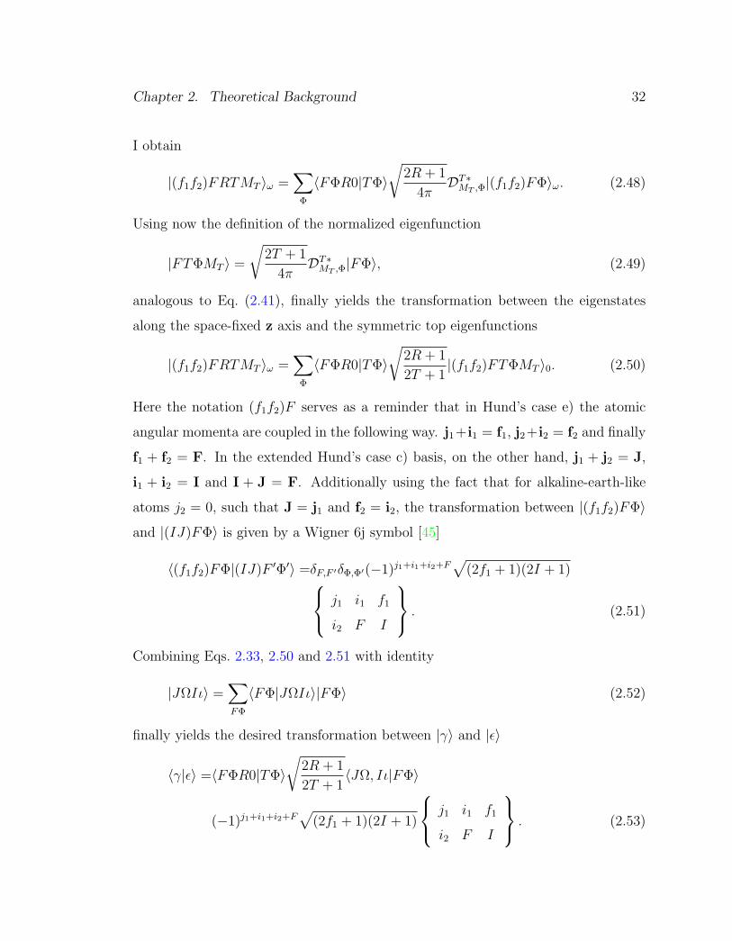
I obtain
|(f1f2)FRTMT 〉ω =∑
Φ
〈FΦR0|TΦ〉√
2R + 1
4πDT∗MT ,Φ
|(f1f2)FΦ〉ω. (2.48)
Using now the definition of the normalized eigenfunction
|FTΦMT 〉 =
√2T + 1
4πDT∗MT ,Φ
|FΦ〉, (2.49)
analogous to Eq. (2.41), finally yields the transformation between the eigenstates
along the space-fixed z axis and the symmetric top eigenfunctions
|(f1f2)FRTMT 〉ω =∑
Φ
〈FΦR0|TΦ〉√
2R + 1
2T + 1|(f1f2)FTΦMT 〉0. (2.50)
Here the notation (f1f2)F serves as a reminder that in Hund’s case e) the atomic
angular momenta are coupled in the following way. j1+i1 = f1, j2+i2 = f2 and finally
f1 + f2 = F. In the extended Hund’s case c) basis, on the other hand, j1 + j2 = J,
i1 + i2 = I and I + J = F. Additionally using the fact that for alkaline-earth-like
atoms j2 = 0, such that J = j1 and f2 = i2, the transformation between |(f1f2)FΦ〉
and |(IJ)FΦ〉 is given by a Wigner 6j symbol [45]
〈(f1f2)FΦ|(IJ)F ′Φ′〉 =δF,F ′δΦ,Φ′(−1)j1+i1+i2+F√
(2f1 + 1)(2I + 1) j1 i1 f1
i2 F I
. (2.51)
Combining Eqs. 2.33, 2.50 and 2.51 with identity
|JΩIι〉 =∑FΦ
〈FΦ|JΩIι〉|FΦ〉 (2.52)
finally yields the desired transformation between |γ〉 and |ε〉
〈γ|ε〉 =〈FΦR0|TΦ〉√
2R + 1
2T + 1〈JΩ, Iι|FΦ〉
(−1)j1+i1+i2+F√
(2f1 + 1)(2I + 1)
j1 i1 f1
i2 F I
. (2.53)

Chapter 2. Theoretical Background 33
Figure 2.2: State-independent optical lattices for the manipulation of neutral atoms.Plot of flexible optical lattices used in experiments at NIST. The single wells can betransformed into double wells, a) to d) show different configurations for the differentdouble wells. The pictures 1-4 show how two atoms in neighboring wells can bemoved together in one lattice site, by first merging the two wells to a double welland then transforming the double well to a single well. Figures are taken from [38]and [14], respectively.

Chapter 2. Theoretical Background 34
Ω
j1
j2
J
TR
Figure 2.3: Schematics of Hund’s case c) coupling. j1 and j2 are coupled to give J,which precesses around the internuclear axis and couples together with R to give thetotal angular momentum T. The projection of J and T on the internuclear axis, Ω,is a good quantum number.

Chapter 2. Theoretical Background 35
j1
j2
J
T
R
Figure 2.4: Schematics of Hund’s case e) coupling. j1 and j2 are coupled to giveJ, which couples together with R to give the total angular momentum T. Thedifference between case e) and case c) is that T is not constrained to process aroundthe internuclear axis, thus its projection Ω on the internuclear axis is not a goodquantum number. However, its projection on a space fixed axis, MT , is a goodquantum number.

Chapter 2. Theoretical Background 36
Ω
L S
J
T R
Λ Σ
Figure 2.5: Schematics of Hund’s case a) coupling. L and S are constrained to precessaround the internuclear axis, due to the strong spin-rotation coupling. They coupletogether to give J, which therefore also precesses around the internuclear axis andcouples together with R to give the total angular momentum T. The projectionsof L,S,J and T on the internuclear axis, Λ,Σ,Ω and Ω, respectively, are all goodquantum numbers.
a
z
Figure 2.6: The classical motion of a prolate symmetric top, where a is the body-fixed axis while z denotes the space-fixed axis. The two cones rotate around eachother without slipping, while the top rotates with angular momentum ω. Compareto [42].

37
Chapter 3
Cooling Atomic Vibration without
Decohering Qubits
3.1 Theoretical Background
From the perspective of storing and manipulating quantum information, nuclear
spins in atoms are attractive given their long coherence times, the mature techniques
of NMR [23] and the collisional gate based on the exchange blockade as described
in Section 2.2. However, as is typical in atomic quantum logic protocols, heating
of atomic motion degrades performance and coherence times. Since qubits usually
experience heating in the process of quantum gates, a truly scalable quantum com-
puter, requiring many such gates necessitates the ability to recool qubits between or
during quantum gates, without disturbing their coherence.
In atoms with group-I-like electronic structures, the qubits are usually stored in
hyperfine levels or other electronic spin states. Therefore, laser cooling cannot be
used to re-initialize atomic vibration in the course of quantum evolution because
this is accompanied by optical pumping that erases the qubit stored in these internal

Chapter 3. Cooling Atomic Vibration without Decohering Qubits 38
degrees of freedom. One must therefore resort to sympathetic cooling with another
species. This cooling mechanism has been successfully used for trapped ions, in
which case two or more ions (one cooling ion and one or more qubit-storing ions) are
in a collective motional mode, and the cooling ion is then laser cooled. Due to the
coupling of the motional mode, the qubit ion(s) are also cooled [46]. Preservation of
the coherence of the qubit(s) can be achieved by either focusing the cooling beam
enough to only illuminate the cooling ion, or by using another species of ions, whose
cooling linewidth is sufficiently detuned from transitions in the qubit species, for the
cooling ion. The lack of long range interactions in neutral atoms, while increasing
their coherence times, also make this form of sympathetic cooling impossible. A way
of implementing sympathetic cooling is to immerse the neutral atoms in a BEC of
another species that acts as a bath, dissipating vibrational motion via the excitation
of phonons [47]. However, this requires the addition and control of a BEC to the
experiment, thus complicating the setup.
For alkaline-earth-like atoms, on the other hand, one can continuously refriger-
ate atomic motion while simultaneously maintaining quantum coherence stored in
nuclear spins, as I will show in this Chapter. The proposed protocol is based on
resolved-sideband laser cooling [48] of group-II-like atoms, tightly trapped in the
Lamb-Dicke regime, as in optical lattices currently under consideration for next-
generation atomic clocks based on optical frequency standards [49]. The cooling
scheme will be explained in detail using two example species, 171Yb and 87Sr, both of
which are actively studied in the laboratory for application to optical clocks [50, 51].
The i = 1/2 nucleus of 171Yb is a natural qubit for storing quantum information. In
the case of 87Sr, whose nucleus has spin i = 9/2, two sublevels in the 10-dimensional
manifold can be chosen to encode a qubit. Exquisite optical control of the nuclear
spin of 87Sr has recently been demonstrated by Boyd et al. [52, 24].
In order to preserve the quantum state of a qubit encoded in a nuclear spin while
laser cooling, the spin coherences must be coherently transferred in both excitation

Chapter 3. Cooling Atomic Vibration without Decohering Qubits 39
and spontaneous decay. Optical fields interacting with atoms via the electric dipole
couple directly to the electrons, affecting nuclear spin states only indirectly via the
hyperfine interaction. A key requirement of our protocol is, therefore, to excite states
with negligible hyperfine coupling, and/or to decouple electrons from nuclear spin
through the application of a sufficiently strong magnetic field that the Zeeman effect
on the electrons dominates over the hyperfine interaction (Paschen-Back regime [53]).
Moreover, we seek to recool atoms in traps to near the ground vibrational state which
requires resolvable motional sidebands, as will be reviewed in the next section.
3.1.1 Resolved Sideband Cooling
In this section, I will give an overview of the well known [54, 55] and frequently
used [56, 57] resolved sideband cooling, which is at the heart of our cooling scheme.
Consider a two-level atom, that is tightly confined in a harmonic oscillator with the
trap frequency ω, which is identical for both the excited state |e〉 and the ground
state |g〉, achievable by trapping the atom in a deep optical lattice at the “magic
wavelength”, such that the two states see the same optical potential. The overall
state is then a product state between the internal state of the atom, |g〉 or |e〉, and
the vibrational state of the trap, |n〉. Under the condition that ω Γ, where Γ is
the linewidth of |e〉, the different vibrational states of the trap, that is the sidebands,
are resolved.
Assuming a one dimensional trap and an incoming plane wave in the same direc-
tion x, the overall Hamiltonian is given by
H = HA +HAL +HT , (3.1)
where HA is the Hamiltonian describing the internal states of the two-level atom,
HAL is the Hamiltonian of the atom-laser interaction and HT gives the harmonic

Chapter 3. Cooling Atomic Vibration without Decohering Qubits 40
oscillator trap. The atomic Hamiltonian can be written as
HA = ωg|g〉〈g|+ ωe|e〉〈e| (3.2)
Shifting the zeropoint of energy by −~(ωe +ωg)/2, and defining ω = (ωe−ωg)/2, we
obtain
HA = ~ω
2(|e〉〈e| − |g〉〈g|) = ~
ω
2σz, (3.3)
where σz is the Pauli matrix [58]. The trapping Hamiltonian is a harmonic oscillator
with oscillation frequency ν, where the a and a† are the annihilation and creation
operators for vibrational excitation in the trap,
HT = ~ν(a†a+
1
2
). (3.4)
The incoming plane wave can be written as
E(x, t) = E0εL[ei(kx−ωLt+φ) + e−i(kx−ωLt+φ)
], (3.5)
where εL is the polarization direction of the incoming wave, while E0, ωL and φ
are its amplitude, frequency and phase. In the dipole approximation, the interaction
Hamiltonian HAL can then be written as HAL = −(d ·εL)E0[exp(kx−ωLt+φ)+c.c.],
which can be expanded in terms of the atomic eigenstates as
(d · εL) = 〈e|d · εL|g〉|e〉〈g|+ 〈g|d · εL|e〉|g〉〈e| = −deg(|e〉〈g|+ |g〉〈e|), (3.6)
where deg = 〈e|d · εL|g〉 = 〈g|d · εL|e〉∗ = 〈g|d · εL|e〉 is the dipole matrix element.
Defining now the Rabi frequency Ω = 2degE0/~ and using the identity of the Pauli
matrices, |e〉〈g| = σ+ and |g〉〈e| = σ−, the interaction Hamiltonian becomes
HAL = −~Ω
2(σ+ + σ−)
(ei(kx−φ)e−iωLt + e−i(kx−φ)eiωLt
). (3.7)
To further simplify this Hamiltonian, it is useful to go to a rotating frame, trans-
forming the Hamiltonian with
H = D†HD + i~∂D†
∂tD, (3.8)
Chapter 3. Cooling Atomic Vibration without Decohering Qubits 41
where D = exp[−(i/~)(HT +HA)t] = exp[−i(ωσzt/2 + ν(a†a + 1/2))]. For the
interaction Hamiltonian, this yields
HAL =D†HALD = −~Ω
2e−i(ω/2)σzt(σ+ + σ−)ei(ω/2)σzt
× e(i/~)HT t(ei(kx−φ)e−iωLt + e−i(kx−φ)eiωLt
)e−(i/~)HT t. (3.9)
Now we use that ei(ω/2)tσzσ±e−i(ω/2)tσz = e±iωtσ±. Furthermore, since the atom is
trapped, x = x0(a+ a†) and the second part of the transformation amounts to going
to the Heisenberg picture with
e(i/~)HT tae−(i/~)HT t = ae−νt. (3.10)
Therefore, the interaction Hamiltonian in the rotating frame is given by
HAL =− ~Ω
2
[σ+e
−i(ω−ωL)t exp[ikx0(ae(−iνt) + a†e(iνt)]e−iφ
σ+e−i(ω+ωL)t exp[−ikx0(ae(−iνt) + a†e(iνt)]eiφ
]+H.c. (3.11)
The two parts of the Hamiltonian have very different resonance frequencies, the first
part oscillates slowly with the detuning of the laser from the resonance frequency
δ = ω−ωL, while the second part oscillates rapidly with ω+ωL. In the rotating wave
approximation the second part can be neglected, so that the interaction Hamiltonian
finally becomes [55]
HAL =~Ω
2σ+ exp
(iη(ae−iωt + a†e−iωt
))ei(φ−δt) +H.c., (3.12)
where
η = kx0 =
√ER~ν
(3.13)
is the Lamb-Dicke parameter with the recoil energy ER = (~k)2/2m. In the Lamb-
Dicke regime, where the confinement is tight and η 1, this Hamiltonian can be
expanded in lowest order in η and be written in the form [55]
HAL = Hcar +Hrsb +Hbsb, (3.14)

Chapter 3. Cooling Atomic Vibration without Decohering Qubits 42
where the zeroth-order part of the Hamiltonian,
Hcar =~Ω
2
(σ+e
iφ + σ−e−iφ) (3.15)
describes the carrier resonance, which couples the atomic excited and ground state to
each other, without changing the vibrational frequency of the trap, |g〉|n〉 ↔ |e〉|n〉.
The first-order part of the Hamiltonian consists of two different parts, the first of
which is the red sideband Hamiltonian
Hrsb =~Ω
2η(aσ+e
iφ + a†σ−e−iφ) , (3.16)
which describes transitions from ground to excited state, reduced by one quantum
of vibration, |g〉|n〉 ↔ |e〉|n− 1〉. It gives rise to a resulting Rabi frequency of
Ωn,n−1 = Ωη√n. (3.17)
The second first oder term of the Hamiltonian is the blue sideband Hamiltonian
Hbsb =~Ω
2η(a†σ+e
iφ + aσ−e−iφ) , (3.18)
which gives rise to transitions |g〉|n〉 ↔ |e〉|n+ 1〉, with a Rabi frequency of
Ωn,n+1 = Ωη√n+ 1. (3.19)
If the Rabi frequency and the linewidth are now small enough, such that the
sidebands are resolved during the excitation, Ωn,m,Γ ω, it is possible to resonantly
excite the atoms on the first red sideband, |g〉|n〉 → |e〉|n− 1〉 while not exciting the
carrier or other sidebands. However, to the degree to which the system is in the
Lamb-Dicke regime where η 1, decay from the excited state will predominantly
be on the carrier, |e〉|n−1〉 → |g〉|n−1〉, which is zeroth order in η. Since the resulting
transition yields |g〉|n〉 → |g〉|n− 1〉, this can be used to cool the vibrational state of
the trapped atoms by repeating this cycling transition. The rate Rn for this process is
found by determining the probability of the atom to be in the excited electronic state
Chapter 3. Cooling Atomic Vibration without Decohering Qubits 43
multiplied with the decay rate. This can be calculated using the master equation in
Lindblad form for the two levels of the atom, which has the following form
ρ = − i~
[H, ρ] + Lρ. (3.20)
The first part of the equation, − i~ [H, ρ] describes the unitary evolution while Lρ
describes spontaneous emission and can be expressed as [59]
Lρ = − Γ
2(σ+σ−ρ+ ρσ+σ− − 2σ−ρσ+), (3.21)
where Γ is a general linewidth. Using a general Hamiltonian, similar to (3.15), but
with a detuning δ and a general Rabi frequency Ω, the resulting equations for the
density matrix are
ρee = −ρgg = −Γρee + iΩ
2Imρge (3.22a)
ρge =
(−iδ − Γ
2
)ρge − Ω(ρee − ρgg) (3.22b)
In the steady state, in which ρ = 0, we can solve for the populations
ρge = − iΩ/2
iδ + Γ/2(ρee − ρgg) (3.23a)
ρee = −Ω
ΓImρge =
−Ω2/4
δ2 + Γ2/2(2ρee − 1) =
Ω2
Γ2 + 2Ω2 + δ2(3.23b)
For excitation on the red sideband, the general Rabi frequency Ω from (3.23b)
becomes Ωn,n−1 = Ω√nη (see Eq. (3.17)), the general linewidth Γ becomes the
natural linewidth of the excited state Γ, and the detuning δ = 0. Therefore, the rate
Rcool for this process is given by
Rcool = Γρee = ΓΩ2n,n−1
Γ2 + 2Ω2n,n−1
= ΓΩ2nη2
Γ2 + 2Ω2nη2≈ Ω2nη2
Γ. (3.24)
It can be seen that the ground vibrational state is a dark state.
Heating of the ground state is possible in two different ways, the first of which
is off-resonant excitation (δ = ω) on the carrier with Ω = Ω0,0, followed by decay

Chapter 3. Cooling Atomic Vibration without Decohering Qubits 44
on the blue sideband. Since this decay changes the vibrational state of the atom,
the linewidth is reduced by the square of the Lamb-Dicke factor and is therefore
Γ = η2Γ (where η is the Lamb-Dicke parameter for decay, slightly different from η
for geometrical reasons [55]). Again using R = Γρee, the rate for this heating process
is
Rheat,1 = ΓΩ2
0,0
Γ2 + 2Ω20,0 + 4δ2
≈ η2ΓΩ2
4ω2. (3.25)
The other heating process is off-resonant excitation (δ = 2ω, Ω = Ω0,1) on the blue
sideband and decay on the carrier, for which the rate is [55]
Rheat,2 = ΓΩ2
0,1
Γ2 + 2Ω20,1 + 4δ2
≈ Γ(ηΩ)2
4(2ω)2. (3.26)
All other heating mechanisms are of higher order in the Lamb-Dicke parameter and
can therefore be neglected. Since the overall heating rate Rheat = Rheat,1 + Rheat,2,
the resulting rate equations for the ground and first excited vibrational state are
given by
p0 = p1Rcool − p0Rheat = p1(ηΩ)2
Γ− p0
[(Ω
2ω
)2
η2Γ +
(ηΩ
4ω
)2
Γ
], (3.27)
p1 = −p0.
This results in an average excitation number of
〈n〉 ≈ p1 ≈(
Γ
2ω
)2[(
η
η
)2
+1
4
], (3.28)
assuming the system to be in steady state and using ω Γ. The factor in brackets
is of order one. Eq.(3.28) shows that resolved sideband cooling can lead to very low
temperatures for forbidden lines, which will be used in the cooling scheme.
3.2 Description of the Proposed Cooling Scheme
The dual requirement of very narrow linewidths and small hyperfine coupling leads us
to consider cooling on the weakly allowed intercombination “clock” transition 1S0 →
Chapter 3. Cooling Atomic Vibration without Decohering Qubits 45
3P0 in a “magic wavelength” optical lattice [49]. Cooling to the ground vibrational
state can proceed by coherent excitation of a π pulse on the first red sideband,
|1S0, n〉 → |3P0, n − 1〉, where n is the vibrational quantum number, followed by
recycling to the ground state with Lamb-Dicke suppression of recoil.
3.2.1 Resolved Sideband Cooling on the Clock Transition
Our concern is to carry out this cooling while maintaining nuclear spin coherence. To
good approximation, the 3P0 state has total electron angular momentum j = 0, and
under this condition, there is no interaction between electrons and nuclear spin, as
in the ground state, |1S0〉. However, the clock transition is j = 0→ j = 0, and laser
excitation is only allowed because in the excited state, the hyperfine interaction leads
to a small admixture of the higher-lying P states as described in 1.3. The nuclear
spin projection mi is thus not an exact quantum number for the magnetic sublevels
in |3P0〉; a very small admixture of electronic angular momentum renders mf a good
quantum number. This leads to two effects which we must address in the context
of transferring the nuclear spin state. While the clock transition is only allowed due
to the hyperfine interaction, it is still the case that the sublevels of |3P0〉 are almost
pure mi, and a π-polarized pulse will preserve nuclear spin projections in excitation
on the clock transition [24]. More importantly, even a small admixture of electron
angular momentum can strongly affect the magnetic moment, so that the g-factor of
the excited state differs from that of the ground state [52]. This implies that in a bias
magnetic field, the π-transitions |1S0, n〉⊗ |mi〉 → |3P0, n− 1〉⊗ |mf = mi〉 will have
different resonant frequencies for different values of mi. The protocol for the transfer
of nuclear spin coherence from the ground state to the clock state will thus depend
on the details of the experimental conditions, i.e., the relative size of the differential
Zeeman splitting in the given bias field when compared to the vibrational spacing
in the trap. Under any operating condition, these coherences can be transfered due
to the extremely narrow linewidth of the clock transition, be it through sequential

Chapter 3. Cooling Atomic Vibration without Decohering Qubits 46
addressing of each sublevel in a series of narrow band pulses [52], or in a short pulse
that does not resolve the differential Zeeman shift but does resolve the sidebands.
Finally, in this step, one must also take into account that the differential g-factor leads
to differential relative phases between the sublevels; this is a unitary transformation
which can be reversed.
Once the atom is transferred to the clock state 3P0, the cooling cycle must be
completed through a spontaneous event that returns the atom to its ground electronic
state 1S0, with Lamb-Dicke suppression of recoil. Of importance in our protocol is
that this occurs without decoherence of the nuclear spin state. The key require-
ment for spontaneous transfer of coherences is that the decay paths of the different
sublevels are indistinguishable, i.e. the decay channels cannot be distinguished by
their polarization or frequency. Under circumstances in which the nuclear spin and
electronic degrees of freedom of an excited state are decoupled (no hyperfine in-
teraction), in a product state with zero projection of electron angular momentum,
|e〉 ≈ |i,m′i〉 ⊗ |j′,m′j = 0〉, all decay channels to the ground state are indistin-
guishable. To see this, note that the selection rules dictate that the electric dipole
matrix element satisfies, 〈e|dq|g〉 = 〈j′,m′j = 0|d0|j = 0,mj = 0〉δq,0δmi,m′i. Only
π-transitions are allowed and all decay channels have the same polarization without
change of nuclear spin projection. Moreover, in the m′j = 0 manifold, the g-factor
is solely nuclear, gI , equivalent to that in the ground state. Thus, the Zeeman
splitting in excited and ground states will be equal and decay channels will not be
distinguished by frequency. Deviations of the excited state from a nuclear-electron
product state (due to residual hyperfine interaction) will lead to decoherence when
there are nuclear spin changing decays (polarization distinguishable) and/or when
the different channels are frequency resolvable (i.e. have a frequency difference that
is not negligible compared to the decay linewidth).
In the case of the clock state 3P0, spontaneous decay is completely due to the
admixture of higher P states and the decay channels with different polarizations

Chapter 3. Cooling Atomic Vibration without Decohering Qubits 47
occur with a probability proportional to the respective Clebsch Gordan coefficients.
Therefore, the nuclear spin is not preserved during spontaneous decay. Moreover,
the long lifetime makes the cooling cycle too long for practical purposes. We thus
consider quenching the clock state by pumping to the short lived 1P1 state (see
Fig. 3.2) [60, 61]. This level decays with very high probability to the ground state
1S0 and has a very broad linewidth, Γ/(2π) > 10 MHz. Direct excitation 3P0 →1P1, is weakly magnetic-dipole-allowed, and has been considered in the context of
electromagnetically induced transparency [26]. Alternatively, we can quench the
clock state via a two-photon 3P0 → 3S1 → 1P1(mj = 0) transition, off resonance
from the intermediate state. This has the advantage that, though one leg is an
intercombination line, all transitions are electric-dipole allowed, leading to larger
depopulation rates for the same intensity.
3.2.2 Quenching of a Metastable State via a Rapidly Decay-
ing State
For the aforementioned reasons, the proposed cooling scheme requires quenching with
a rapidly decaying state. Therefore, in this section, I will discuss different schemes to
quench a metastable excited state |2〉 with a rapidly decaying excited state |3〉, which
has a very large decay rate Γ and decays only to the ground state |1〉. The energy
of state |i〉 = ~ωi, where the ground state energy is set to zero, ω1 = 0. For our
purposes, |1〉 = |1S0〉, |2〉 = |3P0〉 and |3〉 = |1P1〉. There are two different ways of
achieving quenching, one can either dress the metastable state via a continuous-wave
laser with the excited state |3〉, thus broadening its lifetime, or one can coherently
transfer the population from |2〉 to |3〉 and let |3〉 decay back to the ground state.
Here I want to elucidate these different schemes if the Rabi frequency Ω with which
we can couple |2〉 and |3〉 is small compared to Γ, and to estimate required intensities
for implementation of the processes.

Chapter 3. Cooling Atomic Vibration without Decohering Qubits 48
Continuous wave
Consider the excited subspace consisting of states |2〉 and |3〉, which are magnetic-
dipole coupled to each other with a laser resulting in the Rabi frequency Ω =
|〈3|µ|2〉|B0/~, where B0 is the magnetic field and µ is the magnetic dipole moment.
For Sr, µ = 0.022µB [26], while the value for Yb has not been determined, but is
expected to be of similar magnitude. The Hamiltonian of this system in the rotating
frame, after applying the rotating wave approximation is similar to the Hamiltonian
for the carrier, Eq. (3.15)
H =~Ω
2
(σ+e
i(φ−iδt) + σ−e−i(φ−δt)) . (3.29)
where δ is the detuning of the dressing laser. Following [26], the resulting equations
of motion are
c2(t) = −iΩ2eiδtc3(t) (3.30a)
c3(t) = −iΩ2eiδtc2(t)− iΓ
2c3(t), (3.30b)
This causes causes some admixture of the state |3〉 to |3〉 and conversely, the state
|2〉 is dressed with the state |3〉. In leading order in Ω/(δ + iΓ/2) this gives
|2〉 =[|2〉e−iω2t + b|3〉e−i(ω3+δ)t
]e−iβt (3.31)
with b = Ω2(δ+iΓ)
and β = 12Ωb. On resonance with δ = 0, the decay rate of |2〉 is
Γ =Ω2
Γ. (3.32)
Assuming a linewidth of Γ/(2π) = 28 MHz for the excited state, an intensity of
I = 1.1kW/cm2 is required to achieve a effective decay rate of Γ = 1 kHz, fast
compared to the coherence times of nuclear spins of alkaline-earth-like atoms, which
can be up to a second [52].
Note that Γ is inversely proportional to Γ, so the faster |3〉 decays, the smaller
the resulting linewidth of the dressed state. This is an example of the Zeno effect,

Chapter 3. Cooling Atomic Vibration without Decohering Qubits 49
in that the decay of |3〉 probes whether or not the population from state |2〉 was
pumped out [62]. Therefore, quenching via states with smaller linewidths can be
advantageous under certain circumstances.
Pulsed scheme
An alternative approach to quenching is to use pulses of light to transfer the popu-
lation from the metastable state to the rapidly decaying state. Here I will examine
a scheme where we have several pulses with duration τ1 < 1/Γ separated by a time
τ2 > 1/Γ to answer the question whether it is possible to achieve a higher pumpout
rate than with a cw pulse with duration t, assuming that the energy input of the
laser is held constant. To this end, I use again the master equation in Lindblad form,
given in Eq. (3.20).
In this case, we assume that there is no coupling between states |3〉 and |1〉, which
is a good approximation, given that Γ = Γ3 is six orders of magnitude bigger than Γ2.
Furthermore, |3〉 also decays predominantly to |2〉 and we ignore spontaneous decay
from |3〉 to |2〉, such that σ+ = |3〉〈1|. The Hamiltonian that governs the dynamics
of this process is given in (3.29). Putting this all together yields the following set
of coupled differential equations for the relevant populations and coherences of the
density matrix
ρ11 = Γρ33 (3.33a)
˙ρ22 = ΩIm(ρ23) (3.33b)
˙ρ33 = −ΩIm(ρ23)− Γρ33 (3.33c)
˙ρ23 =iΩ
2(ρ33 − ρ22). (3.33d)

Chapter 3. Cooling Atomic Vibration without Decohering Qubits 50
For small times τ this can simply be integrated to give
ρ11 = Γτρ33 (3.34a)
ρ22 = ΩτIm(ρ23) + ρ22(0) = ΩτIm(ρ23) + 1 (3.34b)
ρ33 = −ΩτIm(ρ23)− Γτρ33 (3.34c)
ρ23 =iΩτ
2(ρ33 − ρ22), (3.34d)
where ρ22(0) = ρ33(0) = 0. For small τ most of the population is still in the
metastable state, ρ22 ≈ 1 and ρ22 ρ33, as can be seen by solving for these popula-
tions, which leads to
ρ11 = ΓΩ2τ 3 (3.35a)
ρ22 = 1− Ω2τ 2. (3.35b)
We assume that the time for the experiment t τ2 τ1, such that there will be
many pulses that transfer population. The original intensity is I0, the intensity of
the short pulses is then I1 = (τ1 + τ2)/τ1I0. The Rabi frequency scales with the
square root of the intensity, therefore the Rabi frequency for the pulses is given by
Ω1 =√
(τ1 + τ2)/τ1Ω. The population which is pumped out of ρ22 with n = t/(τ1+τ2)
pulses is ρ22(0)(1 − c)n = (1 − c)n. According to the equations above c is given by
Ω21τ
21 = Ω2τ 2
1 (τ1 + τ2)/τ1 ≈ Ω2τ1τ2. For small τ1 it follows that n ≈ t/τ2 Putting it
all together gives
ρ22(t) ≈ (1− Ω2τ1τ2)t/τ2 . (3.36)
It can be seen that for τ1 → 0 all the population stays in the ρ22 state. Therefore,
using a pulsed scheme to pump the population out of the metastable state does not
necessarily improve the decay rate if Γ Ω, as long as the intensity times the time
of the pulses is held constant.

Chapter 3. Cooling Atomic Vibration without Decohering Qubits 51
3.2.3 Decoupling the Nuclear Spin from the Electronic De-
grees of Freedom in the Quenching Process
In order to obtain the product states of nuclear-electron spin degrees of freedom in
1P1 as required for preserving nuclear spin coherence, we employ a magnetic field.
The 1P1 subspace is then governed by the Hamiltonian including Zeeman interaction,
magnetic spin coupling and quadrupole effects,
H = Ai · j +Q3(i · j)2 + 3/2i · j− i(i+ 1)j(j + 1)
2ij(2i− 1)(2j − 1)
+ gJµB j ·B− gIµN i ·B, (3.37)
where gJ and gI are the relevant electron and nuclear g-factors. If now the energy
shift due to the magnetic field is large compared to the hyperfine splitting, such that
we are in the Paschen-Back regime, mi and mj become good quantum numbers once
again. The magnetic hyperfine constants are A/h = −216 Mhz and A/h = −3.4
MHz for 171Yb and 87Sr respectively [52, 24, 63].
For 171Yb, because i = 1/2, the quadrupole constant Q = 0 and we can analyt-
ically solve for the energy spectrum and eigenstates. By using Aj · i = A((i+j− +
i−j+)/2 + iz jz), it can be seen that the above Hamiltonian is blockdiagonal in the
basis |i = 1/2,mi = 1/2, j,mf + 1/2〉, |i = 1/2,mi = −1/2, j,mf − 1/2〉 and the
blocks with constant mf can be written as A2(mf− +B[gJµB(mf−)− 1
2gIµN ] A
2
√j(j + 1)−mf+mf−
A2
√j(j + 1)−mf+mf− −A
2(mf+) +B[gJµB(mf+) + 1
2gIµN ]
,
(3.38)
where mf± = mf ±1/2. Solving these blocks leads to a modified Breit-Rabi formula,
Emj ,mi(B) = − EHF
2(2j + 1)+ gJµBBmf ±
EHF
2
√1− 4mfx
2j + 1+ x2, (3.39)

Chapter 3. Cooling Atomic Vibration without Decohering Qubits 52
where x = (gIµB + gJµN)B/EHF, mf = mi +mj and EHF = A(j+ 1/2). This differs
from the standard Breit-Rabi formula, in which j = 1/2 and i is arbitrary, in that i
is replaced by j and the second term as well as the second term in the square root
have opposite signs. The resulting Zeeman diagram can be seen in Fig. 3.3. The
eigenstates are specified by
|mf〉 =∑q
cq,mf |mi = mf − q〉|mj = q〉, (3.40)
for q = 0, 1,−1, with field dependent expansion coefficients cq,mf . For high magnetic
fields, in the subspace of interest, c0,mf → 1, as can be seen in Fig. 3.4, and the
states are in a product state |mi〉 ⊗ |mj = 0〉. Deviations from this limit lead to the
residual differential g-factor.
Since 87Sr has a large quadrupole constant Q/h = 39 MHz [64], the Breit-Rabi
formula does not apply. Diagonalizing Eq. (3.37) numerically gives the Zeeman
diagram shown in Fig. 3.3 (for an analytic form, see [24]). Each of the three subspaces
for mj = 1, 0,−1 consists of 10 sublevels which asymptote to the 2i + 1 projections
associated with the nuclear spin of this isotope, i = 9/2. For fields of order 10
mT or greater the Zeeman effect dominates over the hyperfine coupling and the
sublevels approach product states of electron and nuclear spin. However, the residual
quadrupole interaction leads to a complex spectrum that is not described by a linear
Zeeman shift with an effective g-factor. For B-fields between 50 and 120 mT, the
subspace with mj=0 is nearly flat. Additionally, due to the quadrupole symmetry,
the states with equal |mi| are paired and very close in energy (less than 2 MHz),
whereas the energy splitting between the pairs is on the order of tens of megahertz,
nearly as big as the linewidth. Given the near degeneracy of the sublevels ±mi, we
will consider preserving nuclear spin coherence in a qubit encoded in one of these
two-dimensional subspaces, thereby ensuring that the frequencies of the different
decay channels are not resolvable.

Chapter 3. Cooling Atomic Vibration without Decohering Qubits 53
3.3 Results
In the following, I quantitatively study the transfer of nuclear spin-coherence via
spontaneous emission. Consider a qubit in the excited state α|e, ↑〉 + β|e, ↓〉 which
decays to the ground state |g〉. We wish to transfer the qubit into the superposition
α|g, ↑〉 + β|g, ↓〉. Here |e, ↑(↓)〉 = |1P1,mf = ±mi〉 and |g, ↑(↓)〉 = |1S0,±mi〉. The
evolution of the atom can be described by a master equation in Lindblad form,
ρ = − i~
[H, ρ]− 1
2
∑q
(L†qLqρ+ ρL†qLq − 2LqρL†q), (3.41)
where
Lq =√
Γ∑mf
cq(mf )|g,mi = mf − q〉〈e,mf | (3.42)
(with cq defined above in (3.40)) are the “jump operators” for the spontaneous emis-
sion of a photon with polarization π, σ+, σ−, (q = 0,+1,−1). Spin coherences,
described by off-diagonal matrix elements, satisfy
ρ(e)↑,↓ = (−i∆e − Γ)ρ
(e)↑,↓ (3.43a)
ρ(g)↑,↓ = −i∆gρ
(g)↑,↓ + Γ′ρ
(e)↑,↓ (3.43b)
where ∆e(g) are the Zeeman splittings of the excited and ground qubits and Γ′ =
Γc0(mf )c0(−mf ). Solving for the ground state coherences in the limit t 1/Γ,
when all population and coherence resides in the ground states,
ρ(g)↑,↓(t) = ρ
(e)↑,↓(0)
Γ′
Γ− iδei∆gt, (3.44)
where δ = ∆g −∆e is the differential energy shift. The parameters δ and Γ′ − Γ are
functions of applied magnetic field, both approaching zero in the perfect Paschen-
Back limit. For finite fields, imperfect decoupling of electron and nuclear spin results
in imperfect transfer of coherences, characterized by the “fidelity”
F = |ρ(g)↑,↓(t)|
2/|ρ(e)↑,↓(0)|2 = Γ′2/(Γ2 + δ2). (3.45)
Chapter 3. Cooling Atomic Vibration without Decohering Qubits 54
The resulting transfer of coherence as a function of the magnetic field can be seen
in Fig. 3.5. For 171Yb, a magnetic field of 1 T is required to reach a fidelity of 99%,
whereas for the ±mi qubit in 87Sr a magnetics field of order 10 mT is sufficient to
obtain this threshold.
Relatively large vibrational frequencies of ν/2π = 90 (260) kHz have already
been realized for Yb (Sr) in an optical lattice in 1D [25, 65]. In principle, given
these tight confinements and the tiny linewidth Γ of the clock transition (few mHz),
the motional sidebands are very well resolved, and extremely cold temperatures
can be reached with a steady state mean vibrational excitation on the order of
〈n〉 ≈ Γ2/(2ν)2 = 10−15 (10−18) [48]. Of course, the true achievable temperature will
depend strongly on the suppression of the different heating mechanisms.
Although I have argued throughout this chapter that one needs to decouple nu-
clear and electronic degrees of freedom in order to preserve nuclear spin coherence
during laser cooling, we still require an interaction that allows for final readout of
the nuclear spin state via resonance fluorescence. Consider first 171Yb. Accord-
ing to Eq. (3.37), the splitting between the |mj,mi = ±1/2〉 states is given by
∆E = gIµNB + Amj, where A is the hyperfine constant for the 1P1 state. Given
171Yb in a magnetic field of 1 T, the splitting between the |mj 6= 0,mi = ±1/2〉 states
is on the order of 200 MHz. The splitting between |↑〉 and |↓〉 in the 1S0 ground state
arises solely due to the Zeeman interaction with the nuclear spin, equal to 7 MHz
for the applied field (gI ≈ 1). The higher the magnetic field, the closer gIµNB is to
Amj and the closer the different splittings are to each other. However, due to the
big hyperfine interaction of 171Yb, huge magnetic fields of tens of T are required for
the two terms to be of the same order. Even more importantly for the purposes of
the readout, the large hyperfine constant causes the difference in the splittings to be
much bigger than the linewidth Γ of the transition. This makes it possible to selec-
tively drive the transition |1S0,mi = +1/2〉 → |1P1,mj = −1,mi = +1/2〉 as shown
in Fig. 3.2 for readout. Furthermore, the states with different mi are decoupled due

Chapter 3. Cooling Atomic Vibration without Decohering Qubits 55
to the magnetic field, as can be seen in Fig. 3.4, thus making a decay process which
switches the sign of mi very unlikely, as in the cooling process. It follows that many
fluorescence cycles can be realized before the nuclear spin of the atom is flipped,
allowing for readout on this line.
For 87Sr in a magnetic field of few mT, the splitting between neighboring substates
in mj = ±1, dominated by the hyperfine interaction, is on the order of the linewidth
and therefore not well resolved. Thus we cannot selectively excite a given mi level in
the same way as described for 171Yb, since invariably both nuclear spin polarizations
that form the basis of the qubit would be excited. We can, however, take advantage
of the difference in the g-factors of the 1S0 and 3P0 states in Sr in order to manipulate
population in the individual magnetic sublevels. Consider a robust control pulse that
transfers all population from 1S0 to 3P0 level. The difference in Zeeman splitting
implies that a narrow-band π-pulse can selectively return population in a chosen mi
level to the ground state, leaving the remaining sublevels shelved in the metastable
clock state. The occupation of level mi can then be probed via fluorescence on the
1S0 → 1P1 transition. The procedure of shelving and activating the state of interest
mi, thus allows us to sequentially measure population in each sublevel.
3.4 Flourescence while Preserving Nuclear Spin
Coherences
In the resolved sideband cooling scheme discussed above, a large magnetic field caused
decoupling between the nuclear spin and the electronic degrees of freedom that were
optically pumped in the process, thus preserving the coherence of the nuclear spins.
However, it is also possible to achieve effective decoupling by virtual coupling to the
excited state using a detuning ∆, which is large compared to the hyperfine splitting,
∆ δEHF . In this case, the hyperfine splitting is not resolved and thus the photon
Chapter 3. Cooling Atomic Vibration without Decohering Qubits 56
scattering is completely elastic, not causing any decoherence, as will be described in
the next paragraph. The disadvantage of this approach is the high intensity required
to excite with a detuning large compared to the hyperfine splitting. This is especially
pronounced for 171Yb, with its large hyperfine splitting. It is also possible to combine
magnetic fields and large detuning to achieve nuclear-spin preserving scattering with
much more relaxed requirements on both the intensity and the required magnetic
fields, as will be shown in this section. This is particularly true when working on the
strong 1S0 → 1P1 transition, where off resonance excitation can still lead to rapid
scattering rates. If one is interested solely in fluorescence of the excited state, eg.
for electronic qubit detection, rather than cooling, such an approach will be useful.
This would for example be the case in the proposal by Gorshkov [66]. The proposal
elucidated here was developed in discussions between S. Rolston from the University
of Maryland and the Joint Quantum Institute (JQI), J. V. Porto from NIST and the
JQI and my advisor I. H. Deutsch and me.
Consider first off-resonant scattering from an excited hyperfine manifold in the
absence of a magnetic field. To find the scattering rate corresponding to absorption of
a laser photon followed by spontaneous emission between magnetic sublevels within
one hyperfine manifold, we use the Kramers-Heisenberg formula
γfm1→fm2
Ω2Γ
4
∑q
∣∣∣∣∣∑f ′
oj′f ′jf
〈fm2|(e∗q ·Df ′f )(ε ·D†f ′f )|fm1〉∆f ′f − iΓ/2
∣∣∣∣∣2
. (3.46)
As usual, Ω is the Rabi frequency, Γ is the linewidth of the excited state and q is the
angular momentum of the photon. Furthermore, ε and e are the polarization of the
laser photon and the spontaneously emitted photon, respectively, while
D†f ′f =∑q,mf
e∗q〈f ′mf + q|fmf ; 1q〉|f ′mf + q〉〈fmf | (3.47)
is the raising operator for the absorption of one photon, and
oj′f ′jf = (2j′ + 1)(2f + 1)
∣∣∣∣∣∣ f ′ i j′
j 1 f
∣∣∣∣∣∣2
(3.48)

Chapter 3. Cooling Atomic Vibration without Decohering Qubits 57
is the relative oscillator strength for the different f → f ′ transitions, with the six-j
symbol .... For 171Yb, o1,1/2,0,1/2 = o1,1/2,0,3/2 = 1. Since we want to preserve the
direction of the nuclear spin and avoid decoherence, only π-polarized light with q = 0
is used for the excitation, however, spontaneous decay can be either via π, σ+ or σ−
light, yielding the scattering rates
γfm→fm−qΩ2Γ
4
∣∣∣∣∣∑f ′
〈f ′m|fm− q; 1q〉〈f ′m|fm; 10〉∆f ′f − iΓ/2
∣∣∣∣∣2
. (3.49)
Inserting the numerical value of the respective Clebsch-Gordan coefficients yields
explicit expressions for spin preserving and spin flipping transitions for Yb,
γ1/2→1/2 =Ω2Γ
4
∣∣∣∣ 1
3(∆− iΓ/2)+
2
3(∆− δEHF − iΓ/2)
∣∣∣∣2 (3.50a)
γ1/2→−1/2 =Ω2Γ
4
∣∣∣∣∣ −√
2
3(∆− iΓ/2)+
√2
3(∆− δEHF − iΓ/2)
∣∣∣∣∣2
. (3.50b)
Here, ∆ is the detuning of the laser from the f ′ = 1/2 state, while δEHF ≈ 300
MHz for the 1P1 state of 171Yb, denotes the splitting between the different hyperfine
states. Thus, for detuning large compared to the hyperfine splitting, the resulting
scattering rates go to
γ1/2→1/2 →Ω2Γ
4= γs (3.51a)
γ1/2→−1/2 → 0, (3.51b)
where γs is the scattering rate for unit oscillator strength. The equations for m =
−1/2 differ only by a sign, yielding the same results for large detuning. Therefore,
as stated before, in the limit of large detuning, coherences are preserved.
In the presence of an intermediate magnetic field, both the energy splitting be-
tween the different states as well as their composition changes. As can be seen in
the Breit-Rabi diagram, Fig. 3.3, the states that approach the |mj = 0〉⊗ |mi〉 states
in the Paschen-Back regime, are separated by an energy much smaller than the bare
hyperfine splitting, even for relatively small magnetic fields. Now the laser can be

Chapter 3. Cooling Atomic Vibration without Decohering Qubits 58
tuned relatively close to this manifold, but still with a detuning large compared to
the splitting between the two states, and with a much larger detuning to the other
manifolds with different mj. Excitation to the states in other manifolds is then
negligible. Thus, the detuning required to preserve nuclear-spin coherences is much
smaller in the presence of magnetic fields, as is the required intensity for a given
scattering rate. Note that the scattering rates in the presence of a magnetic field
deviate from (3.49), in that the Clebsch-Gordan coefficients in the nominator are
replaced by the c-factors from Eq. (3.40), such that Eqs. (3.50a) and (3.50b) become
γ1/2→1/2 =Ω2Γ
4
∣∣∣∣ c0,1/2c0,1/2
∆1/2,0(B)− iΓ/2+
c−1,1/2c−1,1/2
∆1/2,−1(B)− iΓ/2
∣∣∣∣2 (3.52a)
γ1/2→−1/2 =Ω2Γ
4
∣∣∣∣ c0,1/2c0,−1/2
∆−1/2,0(B)− iΓ/2+
c−1,1/2c1,−1/2
∆−1/2,1(B)− iΓ/2
∣∣∣∣2 . (3.52b)
where ∆mi,mj(B) = ∆− gIµNmiB − Emj ,mi(B), is an abbreviation for the detuning
from the respective line, where Emj ,mi(B) is the relevant solution from the modified
Breit-Rabi formula (3.39), while gIµNmiB gives the Zeeman shift in the ground state.
To avoid causing decoherence in the scattering process, the elastic scattering rate
for mi = 1/2 has to equal the elastic scattering rate for mi = −1/2, otherwise
each scattering process constitutes a weak measurement of the state and causes
decoherence. For sufficiently large magnetic fields B & 50mT, the states asymptoting
to |mj = 0〉 ⊗ |mi〉 are separated by less than the linewidth of the excited state.
When the laser is then tuned in the middle between them, an equal superposition
of those two states will be excited, while excitation to other states is negligible.
Decay from this equal superposition will preserve coherences of the nuclear spin,
and the elastic scattering rates for the two processes will be identical. The scattering
rates for spin preserving and spin flip transitions as functions of detuning for different
magnetic fields, at the saturation intensity at which Ω = Γ/√
2, are shown in Fig. 3.6.
The ratio between the nuclear-spin-preserving scattering rate and the nuclear-spin-
flipping scattering rate is several orders of magnitude, allowing for many scattering

Chapter 3. Cooling Atomic Vibration without Decohering Qubits 59
processes before a spin flip occurs. This scattering process can therefore be used for
readout via flourescence or for the quenching process in resolved sideband cooling as
discussed above.

Chapter 3. Cooling Atomic Vibration without Decohering Qubits 60
∣g⟩
∣e⟩
a)
∣g⟩
∣e⟩
b) c)
∣g⟩
∣e⟩
Figure 3.1: Schematics of resolved sideband cooling a) shows the cooling process,while b) shows heating via excitation on the carrier, followed by decay on the bluesideband. c) shows heating by excitation on the blue sideband followed by decay onthe carrier.
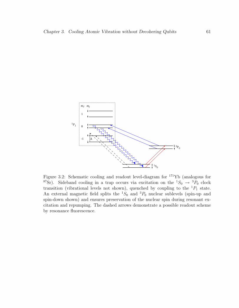
Chapter 3. Cooling Atomic Vibration without Decohering Qubits 61
1
0
-1
mImJ
Δ
1S0
3P0
1P1
Figure 3.2: Schematic cooling and readout level-diagram for 171Yb (analogous for87Sr). Sideband cooling in a trap occurs via excitation on the 1S0 → 3P0 clocktransition (vibrational levels not shown), quenched by coupling to the 1P1 state.An external magnetic field splits the 1S0 and 3P0 nuclear sublevels (spin-up andspin-down shown) and ensures preservation of the nuclear spin during resonant ex-citation and repumping. The dashed arrows demonstrate a possible readout schemeby resonance fluorescence.

Chapter 3. Cooling Atomic Vibration without Decohering Qubits 62
m j = 1
m j = 0
m j = -1
mi = -1 2
mi = -1 2
\ mi = 1 2
mi = 1 2
mi = -1 2
mi = 1 2
¯ \
aL
0 20 40 60 80 100-1.5
-1.0
-0.5
0.0
0.5
1.0
1.5
BHmTL
Eh
HGH
zL
mi = - 9 2
mi = 9 2
mi = 7 2
mi = - 7 2
mi = -5 2
mi = 5 2
mi = ± 3 2mi = ± 1 2
bL
0 20 40 60 80
-20
-10
0
10
BHmTL
Eh
HMH
zL
Figure 3.3: Zeeman diagram of the 1P1 manifold. (a) In 171Yb a slightly modifiedversion of the Breit-Rabi formula applies. The hyperfine sublevels decouple to prod-uct states of electron and nuclear spin (Paschen-Back) with modified linear Zeemanshift. The qubit is encoded in the states |↑〉 and |↓〉 in the mj = 0, subspace. (b)87Sr Zeeman diagram for the 2i + 1 = 10 sublevels that asymptote to the mj = 0subspace in the Paschen-Back regime (other subspaces not shown). Because of thelarge quadrupole effect, pairs with ±mi are closely spaced for magnetic fields between50 and 120 mT. Qubits can be encoded in these pairs without loosing coherence inspontaneous emission.
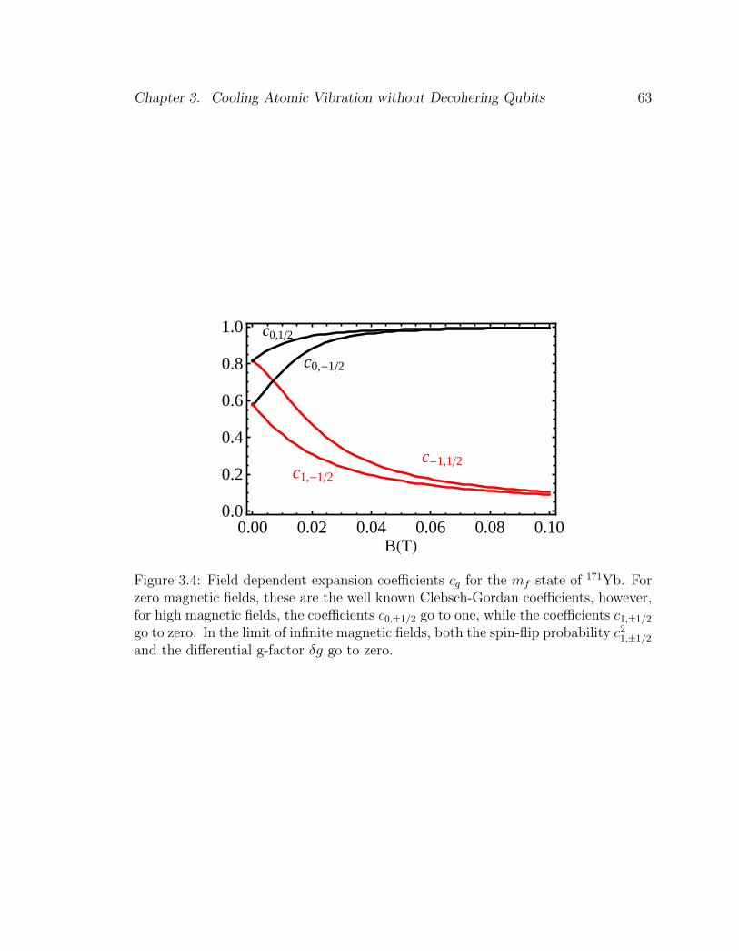
Chapter 3. Cooling Atomic Vibration without Decohering Qubits 63
c0,12
c0,-12
c-1,12c1,-12
0.00 0.02 0.04 0.06 0.08 0.100.0
0.2
0.4
0.6
0.8
1.0
BHTL
Figure 3.4: Field dependent expansion coefficients cq for the mf state of 171Yb. Forzero magnetic fields, these are the well known Clebsch-Gordan coefficients, however,for high magnetic fields, the coefficients c0,±1/2 go to one, while the coefficients c1,±1/2
go to zero. In the limit of infinite magnetic fields, both the spin-flip probability c21,±1/2
and the differential g-factor δg go to zero.

Chapter 3. Cooling Atomic Vibration without Decohering Qubits 64
Figure 3.5: Fidelity for transfer of coherence, F = Γ′2/(Γ2 + δ2) (see text), as afunction of magnetic field. (a) The spin-1/2 qubit of 171Yb. (b) Different choices ofqubit encoding as ±mi in 87Sr.

Chapter 3. Cooling Atomic Vibration without Decohering Qubits 65
aL
-300 -200 -100 0 100 200 3000
1
2
3
4
5
6
7
DHMHzL
bL
-400 -200 0 200 4000
2
4
6
8
10
12
DHMHzL
cL
-200 -100 0 100 2000
2
4
6
8
10
12
DHMHzL
dL
-100 -50 0 50 1000
2
4
6
8
10
12
14
DHMHzL
Figure 3.6: Scattering rates (arbitrary units) for the cooling scheme utilizing inter-mediate magnetic fields and large detuning to achieve decoupling of the nuclear spinfrom the electronic degrees of freedom. Shown are the scattering rate γ1/2→1/2 (blue),γ−1/2→−1/2 (green), γ1/2→−1/2 (red) and γ−1/2→1/2 (orange), as a function of the de-tuning relative to the middle between the two states asymptoting to |mj = 0〉⊗|mi〉.The different panels are for different magnetic fields, a) is for a magnetic field of 1mT, b) for 25 mT, c) for 50 mT and d) for 100 mT. For the higher magnetic fieldsthe ratio between the spin-conserving scattering rates to the spin-changing scatteringrates is large.

66
Chapter 4
Optical Feshbach Resonances for
171Yb
4.1 Background
Feshbach resonances, which were first described by Feshbach [67] and Fano [68],
are a very important tool for the manipulation of the scattering properties of two
interacting atoms [35]. They occur when a bound state of one molecular potential, a
closed channel, is energetically close to the threshold of another molecular potential,
an open channel, of the same system (see Fig. 4.1). Under these circumstances, a
scattering state of the second potential can easily be coupled to the molecular bound
state, thus changing its scattering properties and causing the scattering length of the
open channel to go through a pole. Here, the scattering length reaches the unitary
limit, a → ∞. (See also section 2.1.) Off-resonantly, there is still some admixture
of the closed-channel wave function to the open-channel wave function, which is
sufficient to change the scattering length.

Chapter 4. Optical Feshbach Resonances for 171Yb 67
relative distance
E
Figure 4.1: Schematics of a Feshbach resonance. There are two potentials, one ofwhich has a bound state energetically close to the threshold of the other one. It ispossible to change the relative energy of the two potentials and thus changing thedetuning ∆ between the scattering state and the bound state. For ∆ = 0, the openchannel is resonant with the closed channel and the scattering length diverges.
4.1.1 Feshbach resonances in controlling atom-atom interac-
tions
There is a multitude of applications which are only feasible due to the presence
of Feshbach resonances and the resulting tunability of the scattering interaction
between two atoms. One example is the production of cold molecules via Feshbach
resonances [69], which has been successfully applied for several different species off
alkalis [35]. To this end, the atoms are brought together and then the parameters of
the the experiments are slowly changed, such that the atoms are adiabatically swept
through the Feshbach resonance. The resulting molecules are only weakly bound,
however, they can then be optically transferred to more deeply bound ultracold
molecular states. This is particularly interesting, since it is not possible to laser-
cool molecules, due to the absence of cycling transitions. Additionally, it allows
for the creation of cold polar molecules, whose strong isotropic interaction might

Chapter 4. Optical Feshbach Resonances for 171Yb 68
allow for novel quantum effects [70]. Furthermore, there have been proposals to use
Feshbach resonances in the implementation of quantum information processing in
optical lattices, either by using them to facilitate the interaction between marker
atoms in a superlattice and the memory atoms stored in another lattice [12] or to
create a polar molecule on each lattice site and use these for QIP [71].
Since two-body interactions are the basis of all many-body phenomena, it is not
surprising that Feshbach resonances have also been used to investigate a broad range
of more complex effects, such as the BEC-BCS crossover, where fermionic atoms
form a BCS state on one site of the Feshbach resonance and bosonic molecules form
a BEC on the other [72]. Additionally, Feshbach resonances are useful in controlling
the superfluid-Mott-insulator transition, and they also allow one to change dilute
ultracold gases from being repulsive to being attractive, thus allowing to investigate
the resulting changes of the many-body states of such systems in real time [15, 73].
4.1.2 Magnetic vs. Optical Feshbach resonances
To date, most applied Feshbach resonances were induced through the application of
an external magnetic field. Here the two different channels are different hyperfine
levels in the ground state of alkali atoms, which have different magnetic moments.
Changing the magnetic field therefore changes the position of the bound state relative
to the scattering state, and the resulting scattering length a can be parameterized
as [35]
a = abg
(1− ∆B
B −B0
), (4.1)
where ∆B is the width of the Feshbach resonance, while B0 is its position and abg is
the background scattering length in the absence of a magnetic field.
However, it is also possible to realize optical Feshbach resonances, by using a
laser to couple a scattering ground state to an excited molecular bound state [74, 75].

Chapter 4. Optical Feshbach Resonances for 171Yb 69
This is particularly relevant for alkaline-earths, which do not have different hyperfine
states in their 1S0 ground state and thus do not have magnetic Feshbach resonances.
Furthermore, lasers can be controlled much more easily and faster than magnetic
fields, allowing for unprecedented control over the two-body interactions, including
spatially and temporally varying scattering lengths. On the other hand, big admix-
tures and therefore large changes of the scattering length require a large Condon
factor, that is, good overlap between the bound molecular wave function and the
ground state scattering wave function. To accomplish this, it is necessary to couple
the ground state wave function to long-range states which are very close to dissoci-
ation, where the density of states is high. However, to now control the scattering
length without causing large losses due to photoassociation and spontaneous emis-
sion, the detuning has to be big relative to the linewidth of the state. For alkalis,
due to their relatively broad optical transitions, it is not possible to fulfill all these
conditions at once, leading to substantial losses due to rapid spontaneous emission
[76, 77, 78]. Fortunately, the very narrow intercombination transition of alkaline-
earths allows for their simultaneous fulfillment [79, 80].
In this chapter, I study optical Feshbach resonances for the 1S0 → 3P1 transition
of 171Yb. The underlying models are generally applicable to other alkaline-earths,
however, 171Yb was chosen since its nuclear spin i = 1/2 forms a natural qubit for
quantum information processing. Optical effects in collisions of alkaline-earth-like
atoms have been demonstrated in recent experiments, including photoassociation
spectroscopy in 171Yb [81] and 88Sr [82] and optical Feshbach resonances of the
bosonic isotopes with zero nuclear spin, including 172Yb, 176Yb [80] and 88Sr [83].
I describe here the first multichannel calculation of Feshbach resonances in fermionic
alkaline-earth-like atoms, including excited-state hyperfine structure, and the re-
sulting modification to nuclear-exchange processes that can be controlled through
off-resonant laser excitation.

Chapter 4. Optical Feshbach Resonances for 171Yb 70
4.1.3 Theory of optical Feshbach resonances
Consider a pair of colliding atoms, just above threshold in their ground state inter-
action potential VS. These atoms are illuminated by a laser with energy ~ωL which
is slightly detuned from an excited bound state Eb in an excited bound state poten-
tial VB, such that the detuning ∆ = Eb/~ − ωL, causing coupling between the two
potentials VB and VS with the optical coupling potential
Vopt(IL) = dAE = ~ΓA
√IL
2Isat, (4.2)
where dA is the atomic dipole moment, while E =√
2IL/(cε0) is the electric field
of the laser with the permittivity of vacuum ε0, the intensity of the laser IL and
the speed of light c. Furthermore, Isat = (2π2~ΓAc)/(3λ3) is the atomic saturation
intensity, which is 0.13 mW/cm2 for the intercombination transition in 171Yb, and
ΓA and λ are the linewidth and wavelength of the atomic transition, respectively
[84, 79].
Bohn and Julienne [84] started with this coupling to derive a semianalytic formula
for the scattering length for optical Feshbach resonances. The scattering matrix
resulting from this ansatz is given by
S = e2iδbg∆− i(Γstim − ΓM)/2
∆ + i(Γstim + ΓM)/2, (4.3)
with the background phase shift δbg in the absence of laser light. Here ΓM is the
natural molecular linewidth and Γstim is the linewidth at a finite collision energy,
broadened by stimulated emission to be
Γstim(I) =π
2~|〈b|d · E|E〉|2 = πV 2
opt|〈b|E〉|2 =π
2
(I
Isat
)~Γ2
AfFC . (4.4)
where fFC is the Franck-Condon factor that measures the overlap between the spatial
wave function of the scattering electronic ground state |E〉 at energy E and the bound
excited state |b〉, see Eq. (4.36). Note that this definition of the Franck-Condon factor
includes the spin parts of the wave functions, thus it equals fFCfrot from [79].

Chapter 4. Optical Feshbach Resonances for 171Yb 71
From Eq. (4.3), I want to obtain the optical scattering length, which is generally
of the form
a(∆, I) = abg + aopt(∆, I)− ibopt(∆, I), (4.5)
where abg is the background scattering length in the absence of the radiation, and
both the real part of the optically induced scattering length, aopt(∆, I) and the
imaginary part bopt(∆, I) are functions of the intensity of the radiation I and the
detuning ∆. Inserting Eq. (4.3) into (2.17) with δ → δ − δbg, where δbg is the
background scattering phase shift, which is small for 171Yb, the optically induced
parts of the scattering length are given by
aopt(I,∆) = lopt(I)
(∆ΓM
∆2 + (ΓM + Γstim(I))2/4
)≈ lop(I)
ΓM∆
(4.6)
and
bopt(I,∆) =lopt(I)
2
(Γ2M
∆2 + (ΓM + Γstim(I))2/4
)≈ 1
2lopt(I)
(ΓM∆
)2
. (4.7)
The latter form of the equations is only valid in a regime in which ∆ ΓM and
∆ Γstim, where ΓM is the molecular spontaneous decay rate calculated from the
multichannel wave function. The optical length lopt(I), which is a key parameter
determining the strength of the influence of the laser is given by [85]
lopt(I) = Γstim(I)/(2krΓM), (4.8)
where kr is the relative coordinate wave number for the reduced mass µ.
As Eqs. (4.6) and (4.7) show, the scattering length can only be changed without
the introduction of large losses if ∆ ΓM , which, as mentioned before, is the reason
for the inherent advantage of alkaline-earths over alkalis for the implementation of
optical Feshbach resonances.

Chapter 4. Optical Feshbach Resonances for 171Yb 72
Figure 4.2: S-wave ground state wave functions calculated with the formula by BoGao [86], for a temperature of a) 25µK and b)2 µK. The dashed red line is a sinefunction, shifted by the known scattering length of -2.83 a0. It can be seen that theagreement is excellent.
4.2 Calculation
The prediction of the optical Feshbach scattering length as a function of the laser
intensity and detuning requires a good understanding of both the ground state scat-
tering wave functions and the excited molecular wave functions. This in turn requires
a good understanding of the molecular potentials, including the nuclear spin and the
hyperfine interaction, as well as magnetic fields and rotation.
4.2.1 Ground States
For alkaline-earths, the 1S0 + 1S0 ground state is comparatively simple, in the ab-
sence of nuclear spin there is only one single potential. For isotopes with finite
nuclear spin, these potentials have a multiplicity, however, owing to the lack of hy-
perfine interaction they are not coupled to each other and can therefore be treated as
single channels. For alkaline-earth-like atoms in the ground state, the only nonzero
quantum number are the nuclear spin i and the orbital angular momentum of the

Chapter 4. Optical Feshbach Resonances for 171Yb 73
two nuclei, R that defines the partial wave of the states. 171Yb, with its nuclear spin
of 1/2 is a fermion, thus the total wave function has to be antisymmetric. Since the
parity of the spatial wave function is given by p = (−1)R, it follows that the only
allowed spin state for even partial waves is given by the antisymmetric singlet state
χS.
1√2
(|↓〉A|↑〉B − |↑〉A|↓〉B)⊗ |R,mR〉 = χS ⊗ |R,mR〉, (4.9)
where |↑〉 = |i = 1/2,mi = 1/2〉 and |↓〉 = |i = 1/2,mi = −1/2〉, while A and B
label the two different nuclei. For odd partial waves, on the other hand, the spin
state is in one of the triplet states, that is
1√2
(|↓〉A|↑〉B − |↑〉A|↓〉B)⊗ |R,mR〉 = χT ⊗ |R,mR〉
|↓〉|↓〉|R,mR〉
|↑〉|↑〉|R,mR〉. (4.10)
where the magnitude of I = i1 + i2, I = 1, p = −1 and the magnitude of the total
angular momentum in the ground state T = R + I. For p-waves, where R = 1,
T = 0, 1 or 2.
Because the bulk of the probability amplitude of these wave functions lies away
from the chemical binding region, only the long-range part of the potential, which
can be modeled with a van der Waals C6/r6 potential, influences the shape of the
ground state wave functions. Therefore, we can use the semi-analytic solutions to
such a C6/r6 potential found by Gao [86] to determine these functions. This yields
two linearly independent solutions, g(r) and f(r). The energy-normalized ground
state wave function is then given by
Ψgao(r) =
√2µ
π~2k(f(r)−K0g(r)) . (4.11)
Here K0 is calculated from the scattering length of the ground state potential of
171Yb, via
−ka =K0Zgg − ZfgZff −K0Zgf
, (4.12)

Chapter 4. Optical Feshbach Resonances for 171Yb 74
where Zgg, Zfg, Zff and Zgf are parameters determined by the energy and the C6
coefficient, as described in detail in [86]. The s-wave scattering length for the ground
state of 171Yb was determined by Kitagawa et al. [87] to be a = −0.15 nm=-2.83 a0,
where a0 is the Bohr radius. In the same paper, the C6 coefficient was found to be
C6 = 1932(30) au.
For large r, outside of the range of the van der Waals potential, the wave function
becomes a phase-shifted free scattering state,
Ψgao(r)r→∞−−−→
√2µ
π~2k(sin(kr)− ka cos(kr)) (4.13)
Plots of the resulting s-wave ground state wave functions for 2µK and 25µK can
be seen in Fig. 4.2, together with the long-range wave functions calculated from
the scattering length for the ground state potential. For sufficiently large internu-
clear distance r, the agreement is excellent. For p-waves, the scattering length was
determined from a fit to a numerical calculation with the Numerov method to be
apbg = (tan[δpbg]/k3)1/3 = −116a0.
4.2.2 Excited States
The excited 1S0 + 3P1 molecular states are much more complicated, giving rise to
a multitude of different coupled potentials, and thus requiring a full multichannel
calculation. That is, the different scattering channels are coupled to each other, and
diagonalizing the potential part of the Hamiltonian at each internuclear distance r
will not capture all the interactions. Physically, the scattering interaction can be
seen as a beamsplitter, where the incoming scattering state is split into the different
channels, interacts there with different interaction amplitudes and the different chan-
nels interfere [39]. Thus, the resulting wave functions will have components of more
than one channel and is discussed in more depth in Section 4.3.4. Fully accounting
for this requires diagonalizing the Hamiltonian for all the channels and internuclear
distances at the same time, and is done with a DVR method, as described later.

Chapter 4. Optical Feshbach Resonances for 171Yb 75
We find the overall Hamiltonian by starting with the Born-Oppenheimer po-
tentials, that is, the potentials formed by electrostatic interaction and relativistic
spin-orbit interactions. Since we are interested in the hyperfine structure, including
rotation and magnetic fields, the relevant Hamiltonians are added to the Hund’s case
c) Hamiltonian, such that
H = Hc +HHF +Hrot +Hmag. (4.14)
The first term represents the radial kinetic energy of the nuclei p2r/2µ plus the elec-
tronic Born-Oppenheimer potentials that asymptote to the 1S0+3P1 scattering chan-
nel and define potential curves VΩσ(r), where σ = p(−1)I . These potentials are
modeled through a Lennard-Jones plus dipole-dipole potential,
VΩσ(r) =C12
r12− C6
r6− σC
Ω3
r3, (4.15)
where the parameters are known reasonably well from fits to experimental data as
C6 = 2810 au, C12 = 1.862 × 10⁸ au and C13 = −C0
3/2 = 0.09695 au [40]. The
hyperfine interaction between the electron and nuclear spin is described by
HHF = A(i1 · j1 + i2 · j2) (4.16)
with the hyperfine constant A, using the fact that j1 = 1, i1 = 1/2 and j2 = 0. The
nuclear mechanical rotational part of the Hamiltonian is given by Hrot = ~2
2µr2R(R+
1), with the reduced mass µ, radius r and rotational angular momentum quantum
number R. Finally, in the limit of small magnetic fields, (|µBgfB| A~) such that
we are in the Zeeman regime where the projections of f1 and f2 are good quantum
numbers, the magnetic field part of the Hamiltonian is given by Hmag = µBgf f1 ·B+
µBgf f2 · B where B is the strength of the magnetic field, gf is the Lande g-factor
and µB is the Bohr magneton. Due to the large hyperfine constant of 3.958 GHz
of the 3P1 state of 171Yb, the above condition is fulfilled to a good approximation
for magnetic fields up to several tesla. We neglect the small magnetic dipole-dipole
interactions between nuclei.

Chapter 4. Optical Feshbach Resonances for 171Yb 76
For the given Hamiltonian, the good quantum numbers are the total angular
momentum quantum number T , its projection on the space-fixed quantization axis
MT , and parity due to inversion of all particles p. Here T = F + R, with F = J + I,
where J is the electronic angular momentum (spin and orbital, J = L + S), R is the
nuclear orbital angular momentum describing mechanical rotation of the dimer, and
I is the nuclear spin angular momentum. In addition, by Fermi statistics, the total
wave function must be antisymmetric under exchange of the nuclei, and by exchange
of all particles. In the absence of a magnetic field, F is also a good quantum number.
Other quantum numbers are approximate, depending on the dominant forces. Any
basis of states that is specified by these eigenvalues is constrained by the overall
symmetries. For example, for a separable basis of electron and nuclear orbitals,
(−1)l1+l2+R = p, where l1 = 0, l2 = 1 are the individual atomic electron angular
momenta for the S+P collision.
4.2.3 Channel Bases
As discussed in Sec. 2.3, the overall Hamiltonian matrix can be calculated by defining
several bases, defined by different couplings of the angular momenta of the atoms,
in which the different parts of the Hamiltonian are diagonal. Finding the overall
Hamiltonian matrix then reduces to the application of basis transformations. The
uncoupled atoms have |nlsjmjimi〉 as good quantum numbers, where j = 0 for the
1S0 ground state. In the excited 3P1 state, j and i are coupled to give f , the total
angular momentum of the atom. While there are many different ways in which these
angular momenta can be coupled to each other and to the rotation R of the two
nuclei, only the following three bases are relevant here. Most of the calculation is
done in the |ε〉 basis, which is a Hund’s case e) basis, extended to include the nuclear
spin
|ε〉 = |((f1f2)FR)TMTp〉. (4.17)

Chapter 4. Optical Feshbach Resonances for 171Yb 77
For the excited 1S0 + 3P1 state, we chose the atom with label 2 to be in the ground
state, such that j2 = 0, f2 = i2, for alkaline-earths. F = f1 + f2 is the total angular
momentum of the coupled atoms, with magnitude f1 = 1/2, 3/2 and f2 = 1/2 for the
possible individual atomic angular momenta. This basis is used for the calculation
of the hyperfine part of the Hamiltonian, which is diagonal in this basis and can be
expressed as
HHF = A(i1 · j1 + i2 · j2) = A/2 [f1(f1 + 1)− i1(i1 + 1)− j1(j1 + 1)]
= A/2 [f1(f1 + 1)− 11/4] , (4.18)
where in the last step the fact that i1 = 1/2, j1 = 1 and j2 = 0 was used. Additionally,
the magnetic field Hamiltonian, HB is also diagonal in this basis and becomes HB =
gfmf1µB, for a magnetic field along the z-axis of the space fixed coordinate system.
Another important basis is the uncoupled |π〉 = |f1mf1 , i2mi2 , RmR, p〉 basis,
which is valid for very far separated atoms, such that their electron spin, electronic
orbital angular momentum and nuclear spins are coupled together to give a total
atomic spin fk = jk + ik for each atom k. Additionally, the projection of fk on the
space-fixed axis, mfk is also a good quantum number, as are the rotational quantum
number of the two atoms R and its projection on the space-fixed axis mR. Denoting
|βk〉 = |γkfkmfk〉 = |nk((sklk)jkik)fkmfk〉 (for the atom in the ground state, f = i,
since j = 0) and symmetrizing yields
|π〉 = |(β1β2)ρRmR〉 = (4.19)
=
1√2
[|β1〉A|β2〉B + ρ(−1)R|β2〉A|β1〉B
]⊗ |R,mR〉
|β1〉A|β2〉B ⊗ |R,mR〉
Here ρ = −1 for fermions and the labels A and B denote the different nuclei. As
required, these states are antisymmetric under exchange of atoms A and B. The
parity is given by p = p1p2(−1)R, where pk is the parity of the electron state k,
which is -1 for the 3P1 state and 1 for the 1S0 state. This basis is used to calculate
the matrix elements of the dipole operator between the ground and multichannel

Chapter 4. Optical Feshbach Resonances for 171Yb 78
excited states. These are essential for determining the molecular natural linewidth
as detailed in [85], where the transformation 〈π|ε〉 is also given to be
〈ε|π〉 = δγ′1,γ1
δγ′2,γ2
δf ′1,f1
δf ′2,f2δR′
1R2〈f1f2mf1mf2|FmF 〉〈F ′mFRmR|T,MT 〉Ξε,π′ , (4.20)
where Ξεπ′ =√
2 for γ1f1 = γ2f2 but mf1 6= mf2 and 1 otherwise. In the excited
molecular states, one atom is in the (6s2)1S0 state and the other one in the (6s6p)3P0
state, therefore, Ξε,π′ is always one.
Hmag, which is diagonal in the |π〉 basis, but not in the |ε〉 basis, is then calculated
via
〈ε|Hmag|ε〉 =∑π,π′
〈ε|π〉〈π|Hmag|π′〉〈π′|ε〉. (4.21)
Additionally, the molecular dipole matrix element in the |ε〉 can be calculated with
the |π〉 basis
〈ε|(dmol)q|εg〉 =∑ππg
〈ε|π〉〈π|(dmol)q′ |πg〉〈πg|εg〉, (4.22)
in which it can be reduced to sums of the atomic dipole moment dq
〈π|(dmol)q|πg〉 =δρgρδRgRδRM,gRM
×[〈β1|dq|β1,g〉δβ2β2,g + ρ(−1)R〈β1|dq|β2,g〉δβ2β1,g
](4.23)
for β1 < β2 and
〈π|(dmol)q|πg〉 = δρgρδRgRδRM,gRM√
2〈β1|dq|β1,g〉 (4.24)
for β1 = β2. The following notation is used here. The ground states are labeled with
a subscript g, for the excited state, β2 denotes the an atom in the 1S0 ground state
and β1 is the atom in the 3P1 excited state.
The third basis, denoted by |γ〉, is an extended Hund’s case c) basis, as derived
in section 2.3. The Born-Oppenheimer Hamiltonian, Hc is diagonal in this molecular

Chapter 4. Optical Feshbach Resonances for 171Yb 79
basis for which s1 + s2 = S, l1 + l2 = L,L + S = J and i1 + i2 = I. Furthermore,
I + J = F which is then coupled to rotation of the nuclei R, to give again the total
angular momentum T, F + R = T.
|γ〉 = |JΩIιΦ, TMTp〉 =∑
(JI)FΦ
〈(JI)FΦ|JΩIι〉|(JI)FΦ〉DT∗Φ,MT. (4.25)
Here Φ = Ω + ι where Φ, Ω and ι are the projection of F,J and I on the internuclear
axis and DT∗Φ,MTis the wave function of a symmetric top. Thus, Φ is the projection
of T on the internuclear axis, while MT is its projection on the space fixed axis. For
a similar basis set for alkalis, compare to [85]. The basis transformation between |γ〉
and |ε〉 is given by
〈γ|ε〉 =〈FΦR0|TΦ〉√
2R + 1
2T + 1〈JΩ, Iι|FΦ〉
× (−1)j1+i1+i2+F√
(2f1 + 1)(2I + 1)
j1 i1 f1
i2 F I
, (4.26)
where ... denotes a Wigner 6J-symbol. The gerade/ungerade quantum number σ
is determined by p = σ(−1)I . For a derivation of this transformation see section 2.3.
4.3 Results
4.3.1 Selective Change of a for P-waves and S-waves
As discussed in section 4.2.1, the total nuclear spin for s-wave collisions I=0, as
are all other angular momenta, including the total angular momentum T . The
electronic ground states have a parity of p = (−1)R, which is 1 for s-waves. Since
the dipole operator is odd under parity and has a selection rule of ∆T = 0, 1 with
T = 0→ T = 0 forbidden, the excited state has to have opposite parity p = −1, and
a total angular momentum of T = 1. Therefore, the rotation R of the nuclei in the
excited state has to be even. Given the fact that T = F + R, with F = 0, 1 or 2 and

Chapter 4. Optical Feshbach Resonances for 171Yb 80
40 60 80 100 120
-20
-10
0
10
20
rHa0L
EHG
HzL
Figure 4.3: The excited adiabatic potentials, accessible via for s-wave collisions.These potentials are found by diagonalizing the potential part of the Hamiltonian asa function of the internuclear distance r. They have a total angular momentum ofT = 1 and their parity p = −1. The shown potentials are for no magnetic field, thusthey are degenerate in MT .
because in the excited state we must have (−1)l1+l2+R = p = −1, R can be either 0
or 2 in the excited state. Taking all this into account leads to 15 different basis states
in the |ε〉 basis, which are listed in table 4.1. However, the resulting Hamiltonian is
blockdiagonal in MT , thus there are three different blocks of 5 channels each. In the
absence of a magnetic field, these three blocks are degenerate.
P-wave collisions are naturally more complex than s-wave collisions, given their
higher rotation R = 1 and their triplet nuclear spin I = 1, which allow for T = 0, 1 or
2. Therefore, there are many more accessible excited states with T = 0, 1, 2 or 3, odd
rotation R = 1, 3, 5 and even parity p = 1, leading to 89 different basis states in the |ε〉
basis, as can be seen in table 4.2. The Hamiltonian is again block diagonal in MT and
T , giving rise to 16 different blocks ranging in size from 2×2 to 6×6. In the absence of
magnetic fields, this reduces to 19, (2T+1)-fold degenerate channels. Due to the large
mass of 171Yb, the rotational energy is very small, causing several of the potentials
with different R to be nearly degenerate. For better visualization, the adiabatic

Chapter 4. Optical Feshbach Resonances for 171Yb 81
40 60 80 100 120
-5
0
5
10
rHa0L
EHG
HzL
Figure 4.4: The excited adiabatic potentials for p-wave collisions, analogous to Fig.4.3. Here the total quantum number T = 0 (blue), 1 (green), 2 (red) or 3 (black),causing different multiplicity for the different lines. Due to the small rotationalenergy, several of these lines can not be resolved on this scale, leaving only 8 distinctlines.
potentials are shown in Fig. (4.3) and Fig. (4.4). These potentials are obtained by
diagonalizing the potential part of the Hamiltonian (4.14) for each value of r. While
this gives a good visual understanding of the system, it can not exhibit the diabatic
T f1 F R1 1/2 1 01 1/2 1 21 3/2 1 01 3/2 1 21 3/2 2 2
Table 4.1: The different channels of the |ε〉 basis used in the calculation for the s-wavestates. f2 is always 1/2 and is therefore suppressed. MT , which is also not shown,can be -1, 0, or 1, for each of the states, leading to a total number of 15 differentchannels. In the absence of a magnetic field, each of these states is 3-fold degenerate,yielding 5 different degenerate potentials.

Chapter 4. Optical Feshbach Resonances for 171Yb 82
T f1 F R0 1/2 1 10 3/2 1 11 1/2 0 11 1/2 1 11 3/2 1 11 3/2 2 11 3/2 2 32 1/2 1 12 1/2 1 32 3/2 1 12 3/2 1 32 3/2 2 12 3/2 2 33 1/2 0 33 1/2 1 33 3/2 1 33 3/2 2 13 3/2 2 33 3/2 2 5
Table 4.2: The different channels of the |ε〉 basis used in the calculation for the p-wavestates. MT is suppressed for clarity, however, each of the states has a multiplicityof 2T + 1, yielding 89 different channels. In the absence of a magnetic field, each ofthese states is 2T + 1-fold degenerate, yielding 19 different degenerate potentials.
coupling between the different channels. Therefore, determining wavefunctions and
eigenenergies from these potentials would be necessarily less accurate than the full
multichannel calculation described earlier.
Note that the symmetry and selection rules cause the potentials to be split into
two separate classes, one of which is accessible from s-wave collisions and the other
that is accessible from p-wave collisions. This can be exploited for the independent
manipulation of p-wave and s-wave scattering lengths, by choosing to use a bound
state with parity p = −1, which is far from bound states with a parity of p = 1.
Since this bound state is dark for p-waves, the s-wave scattering length is changed

Chapter 4. Optical Feshbach Resonances for 171Yb 83
Figure 4.5: Adiabatic purely long-range potentials for s-waves, for a magnetic field of1 kG. In the absence of a magnetic field all three potentials are degenerate with theline in the middle. It can be seen that the extremely shallow potentials get shiftedand develop a barrier in the presence of a magnetic field.
more strongly than the p-wave scattering length that has a larger detuning. In
the same manner it is possible manipulate only p-waves or even to use two lasers
simultaneously, one to change s-waves and the other one to change p-waves. By
spatially and/or temporally changing the intensity of these two different Feshbach
lasers, new and interesting avenues in the control of ultracold atoms are opened.
4.3.2 Purely Long-Range States
Of special interest are several purely long-range (plr) potentials. These are potentials
which have both the outer and inner classical turning point at long internuclear
distance. Typically, purely long-range potentials form in a transition regime between
Hund’s cases, where the strength of the spin-orbit coupling is about as large as the
energy difference between the Born-Oppenheimer potentials. This can cause avoided
crossings between the different Born-Oppenheimer potentials, such that the potential

Chapter 4. Optical Feshbach Resonances for 171Yb 84
Figure 4.6: Adiabatic purely long-range potentials for p-waves, again for a magneticfield of 1 kG. While these potentials are also shifted in the presence of the magneticfield, they do not develop barriers. In the absence of a magnetic field, these potentialsform two nearly degenerate potentials, due to their different rotational quantumnumber R.
surface acquires a minimum at large relative distance of the nuclei. Several bound
states of these purely long-range potentials have been observed [39]. Additionally,
at even larger r, it is also possible that the hyperfine interaction causes the same
effect. Due to the smaller hyperfine constant compared to the fine-structure coupling
constant, the resulting potential minimum is even shallower and at larger internuclear
distance. Therefore, in alkalis, the hyperfine interaction is typically too small relative
to the linewidth to observe such purely-long range states. In alkaline-earths, on the
other hand, again due to the narrow intercombination line, and especially in 171Yb
with its large hyperfine constant, these states can be experimentally observed. The
p-wave plr potential was experimentally observed by Enomoto et al. [81] and has a
depth of only 717 MHz, while the s-wave plr potential is even more shallow, it has
a depth of only 59.2 MHz and to date has not been experimentally observed. The
adiabatic purely long-range potentials are shown in Fig. 4.5. The s-wave potential
is triply degenerate in the absence of a magnetic field, with the quantum numbers

Chapter 4. Optical Feshbach Resonances for 171Yb 85
50 100 150 200 250 300 350 4001.2
1.4
1.6
1.8
2.0
rHa0L
VHG
HzL
Figure 4.7: The eigenstates of an adiabatic purely long-range potential for p-wavesin the absence of a magnetic field. All the amplitude of the states is at compara-tively large r. For simplicity, the vibrational states shown are eigenfunctions of theadiabatic potential, similarly to the calculation in [81]. For full multichannel purelylong-range states see Fig. 4.10.
f1 = 3/2, F = 1, R = 2, T = 1,MT = 0,±1. In the presence of a magnetic field,
however, the three degenerate potentials shift relative to each other and they also
change their shape, developing a barrier and thus a possible shape resonance, as
can be seen in Fig. 4.5. There are two nearly degenerate p-wave purely long-range
potentials, one with the quantum numbers f1 = 3/2, F = 2, R = 1, T = 1,MT in the
ε basis and the other one with f1 = 3/2, F = 2, R = 1, T = 3,MT . In the absence of
a magnetic field, the former is triply degenerate, while the latter is 7-fold degenerate.
In the presence of a magnetic field, these potentials are also shifted relative to each
other, lifting the degeneracies, as can be seen in Fig. 4.6, even though, in contrast
to the s-wave purely long-range states, they do not acquire a shape resonance.
While all the states close to dissociation depend mainly on the very long-range
part of the potentials, this effect is even more pronounced for purely long-range
states, given that they are only sensitive to the hyperfine interaction and the long-
range tail of the potential. This allows for very accurate determination of the Cn

Chapter 4. Optical Feshbach Resonances for 171Yb 86
coefficients if the molecular potentials are modeled with Lennard Jones potentials,
including the determination of the C3 coefficient in the excited states, which are
closely related to the lifetime of the excited states. [39]. Furthermore, Enomoto et
al. [81] used this to determine the C6 coefficient for 171Yb, by assuming a molecular
potential which consists only of the C6/r6 part, the hyperfine Hamiltonian HHF and
the resonant dipole interaction resulting in a 1/r3 potential. Diagonalizing this and
perturbatively adding the rotation yields adiabatic potentials, including the purely
long-range states, allows one to solve for the only free parameter, C6. However, these
solutions do not allow for a full multichannel calculation, given that the rotation is
not fully included, nor are all the basis states.
Generally, given that all the amplitude of the purely-long range states is at large
internuclear distance one would expect the purely long-range states to be especially
suitable to the implementation of photoassociation and optical Feshbach resonances
as compared to other states close to dissociation. However, other states at a similar
energy actually have longer range then the purely long-range states, and therefore
the Condon factor between the latter and the ground state is about an order of
magnitude lower than for the former. Thus, the other states are better suited for
these applications.
4.3.3 Excited-State Spectrum
Having obtained the multichannel Hamiltonian as a function of r in the |ε〉 basis, a
discrete variable representation (DVR) method [88, 89] is used to numerically find the
eigenvalues and multichannel wavefunctions. As described by Colbert and Miller [89],
this method is implemented by first choosing an evenly spaced grid ri = a+(b−a)i/N
with N − 1 points, where i is an iterator going from 1 to N − 1 and a and b are the
start and end point of the grid, respectively. The Fourier functions associated with

Chapter 4. Optical Feshbach Resonances for 171Yb 87
Figure 4.8: S-wave spectrum for the bound states of the excited states. The dashed(red) lines are the results experimental results from [81], while the green lines are fromthe full multichannel calculation. It can be seen that the agreement is good. Thereare some additional lines from the multichannel calculation, however, these have veryweak Frank-Condon factors, such that they could not be seen experimentally. Forthe numerical values of the detuning, see also Table 4.3.
this grid are then
φn(r) =
√2
b− asin
[nπ(r − a)
b− a
], (4.27)
with the iterator n = 1, ..., N − 1. These functions are then used to expand the
kinetic energy operator
T = − ~2
2m
d2
dr2, (4.28)
which can be written in terms of the Fourier eigenfunctions of the grid to be
Tii′ = − ~2
2m∆r
N−1∑n=1
φn(ri)φ′′n(r′i), (4.29)
with the grid spacing ∆r = (b − a)/N . Inserting Eq. 4.27 into the above Equation
yields
Tii′ = − ~2
2m
(π
b− a
)22
N
N−1∑n=1
n2 sin
[nπi
N
]sin
[nπi′
N
]. (4.30)

Chapter 4. Optical Feshbach Resonances for 171Yb 88
Figure 4.9: P-wave spectrum for the bound states of the excited states. The dashed(red) lines are the results experimental results from [81], while the solid lines arefrom the full multichannel calculation. As for s-waves, the agreement is good andthere are some additional lines from the multichannel calculation which have verysmall Frank-Condon factors, such that they could not be seen experimentally. Forthe numerical values of the detuning, see also Table 4.4.
Evaluating the sum gives the following formulae for the diagonal and off-diagonal
terms of the kinetic energy matrix
Tii =~2
2m
π2
2(b− a)2
((2N2 + 1)/3− 1
sin2(πi/N)
)(4.31a)
Tii′ =~2
2m
π2(−1)(i−i′)
2(b− a)2
(1
sin2 [π(i− i′)/2N ]− 1
sin2 [π(i+ i′)/2N ]
). (4.31b)
For more details, see Appendix A from [89]. For a single channel, the potential
matrix is a diagonal (N − 1) × (N − 1) matrix, which is added to the potential
energy matrix derived above. For the multichannel problem the grid points and the
different channels are treated on an equal footing, such that the resulting kinetic
energy matrix is N ′ × N ′, where N ′ is the number of grid points times the number
of channels. The diagonalization of the resulting matrix gives the eigenenergies and
the full multichannel eigenfunctions.
The code used for this calculation was written by Julienne and Tiesinga at NIST,
with minor adaptations for the parameters relevant for 171Yb and the required num-
ber of channels. Since the potentials do not change very much at large r, but are
relatively steep at small r, it is advantageous to have more grid points close to the
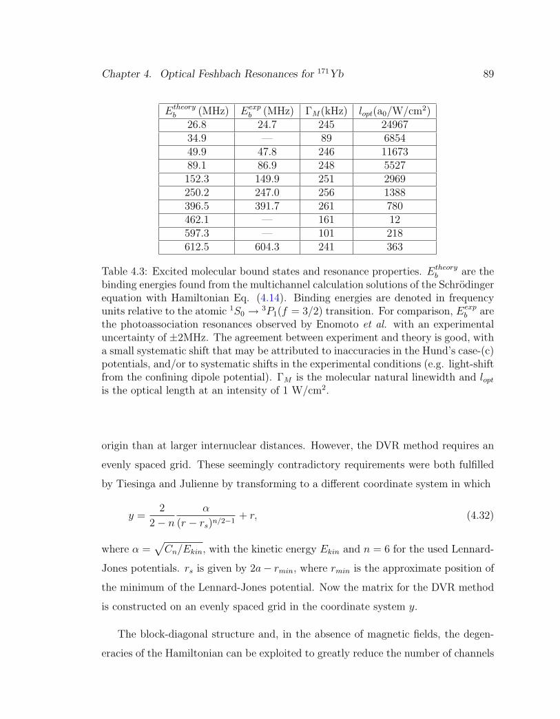
Chapter 4. Optical Feshbach Resonances for 171Yb 89
Etheoryb (MHz) Eexp
b (MHz) ΓM(kHz) lopt(a0/W/cm2)26.8 24.7 245 2496734.9 — 89 685449.9 47.8 246 1167389.1 86.9 248 5527152.3 149.9 251 2969250.2 247.0 256 1388396.5 391.7 261 780462.1 — 161 12597.3 — 101 218612.5 604.3 241 363
Table 4.3: Excited molecular bound states and resonance properties. Etheoryb are the
binding energies found from the multichannel calculation solutions of the Schrodingerequation with Hamiltonian Eq. (4.14). Binding energies are denoted in frequencyunits relative to the atomic 1S0 → 3P1(f = 3/2) transition. For comparison, Eexp
b arethe photoassociation resonances observed by Enomoto et al. with an experimentaluncertainty of ±2MHz. The agreement between experiment and theory is good, witha small systematic shift that may be attributed to inaccuracies in the Hund’s case-(c)potentials, and/or to systematic shifts in the experimental conditions (e.g. light-shiftfrom the confining dipole potential). ΓM is the molecular natural linewidth and loptis the optical length at an intensity of 1 W/cm2.
origin than at larger internuclear distances. However, the DVR method requires an
evenly spaced grid. These seemingly contradictory requirements were both fulfilled
by Tiesinga and Julienne by transforming to a different coordinate system in which
y =2
2− nα
(r − rs)n/2−1+ r, (4.32)
where α =√Cn/Ekin, with the kinetic energy Ekin and n = 6 for the used Lennard-
Jones potentials. rs is given by 2a− rmin, where rmin is the approximate position of
the minimum of the Lennard-Jones potential. Now the matrix for the DVR method
is constructed on an evenly spaced grid in the coordinate system y.
The block-diagonal structure and, in the absence of magnetic fields, the degen-
eracies of the Hamiltonian can be exploited to greatly reduce the number of channels

Chapter 4. Optical Feshbach Resonances for 171Yb 90
and thus the CPU time required to diagonalize the Hamiltonian. For s-waves, the
Hamiltonian can be reduced to one 5×5 matrix, while for p-waves, 4 different blocks
have to be diagonalized, one with T = 0, which consists of two channels, one with
T = 1, which is a 5×5 matrix, and the last two, with T = 2 and T = 3, respectively,
both of which are 6× 6 matrices (compare to table 4.2).
The resulting bound states represent photoassociation resonances that dissociate
to 1S0 + 3P1(f = 3/2). Their positions relative to the atomic resonance were ex-
perimentally determined by Enomoto et al. [81], allowing for comparison between
experiment and the numerical calculation. Fig. (4.8) and Table (4.3) both show re-
sults for s-wave collisions and Fig. (4.9) and Table (4.4) for p-wave collisions. The
agreement is very good. For s-waves, there is a small systematic shift, which could be
caused by the inaccuracies in the Hund’s case c) potentials, or by systematic shifts
in the experiment. However, for p-waves, the numerical calculation agrees with the
experimental results to within the experimental uncertainty. For both s-waves and
p-waves, there are additional lines in the calculated spectrum as compared to the
experimental spectrum, which have not been found by Enomoto et al, either because
their binding is comparable to their lifetime or because they are too tightly bound
and thus have small Franck-Condon factors.
4.3.4 Scattering Length
The DVR method also yields the multichannel eigenvectors of the bound excited
states, which can be described as
|b〉 =∑ε
Ψε(r)|ε〉, (4.33)
where Ψε(r) are the radial eigenfunctions for given partial wave l for channel ε and
|ε〉 are the corresponding spin states in the ε basis. In contrast to the ground state
wave functions, these bound states are unit normalized. These eigenfunctions can
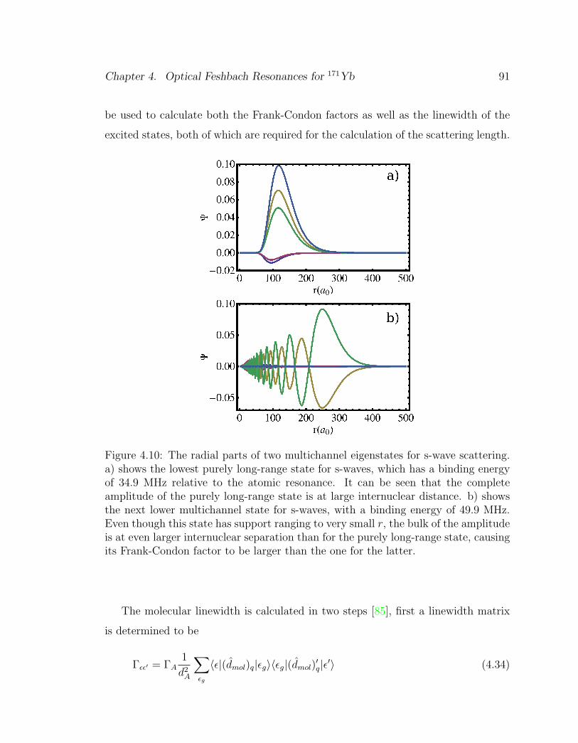
Chapter 4. Optical Feshbach Resonances for 171Yb 91
be used to calculate both the Frank-Condon factors as well as the linewidth of the
excited states, both of which are required for the calculation of the scattering length.
Figure 4.10: The radial parts of two multichannel eigenstates for s-wave scattering.a) shows the lowest purely long-range state for s-waves, which has a binding energyof 34.9 MHz relative to the atomic resonance. It can be seen that the completeamplitude of the purely long-range state is at large internuclear distance. b) showsthe next lower multichannel state for s-waves, with a binding energy of 49.9 MHz.Even though this state has support ranging to very small r, the bulk of the amplitudeis at even larger internuclear separation than for the purely long-range state, causingits Frank-Condon factor to be larger than the one for the latter.
The molecular linewidth is calculated in two steps [85], first a linewidth matrix
is determined to be
Γεε′ = ΓA1
d2A
∑εg
〈ε|(dmol)q|εg〉〈εg|(dmol)′q|ε′〉 (4.34)

Chapter 4. Optical Feshbach Resonances for 171Yb 92
-50 0 50-200
-100
0
100
200
DHMHzL
Figure 4.11: The resulting scattering length for s-wave optical Feshbach resonancesat a temperature of 2 µK. The solid (blue) line is the real part of the scatteringlength, while the dashed (red) line is the imaginary part, which quantizes the losses.
where |ε〉 and |ε′〉 are the spin parts of the basis states for the excited states in the ε
basis, |εg〉 are the spin states of the ground states, q and q′ are the polarization of the
photons, dA is the atomic electric dipole matrix element and dmol is the molecular
dipole operator. The matrix elements of the latter, 〈ε|(dmol)q|εg〉 are calculated by
expanding the states in the π basis, as described by Eqs. (4.23) and (4.24) in section
4.2.3. Now the linewidth of the excited bound state can be obtained by integrating
over the radial part of the wave functions (4.33), multiplied with the relevant elements
of the linewidth matrix (4.34)
ΓM =∑ee′
∫ ∞0
drΨe(r)Γee′Ψe′(r). (4.35)
The resulting linewidths for several s-wave states are shown in table 4.3.
The Franck-Condon factor that measures the overlap between the spatial wave
function of the (energy normalized) scattering ground electron state |g〉 at energy E
and the (unit normalized) bound excited state |b〉 is given by [79]
fFC = |〈b|d · εL|g〉|2 /2d2A, (4.36)

Chapter 4. Optical Feshbach Resonances for 171Yb 93
where dA is the atomic dipole moment for this transition and εL is the laser polar-
ization. Given in Eq. (4.33), Eq. (4.36) can be expanded in the spin part and the
radial part
fFC =
∣∣∣∣∣∑ε
〈εg|dmol|ε〉∫ ∞
0
drΨg(r)Ψ∗ε(r)
∣∣∣∣∣2
/2d2A, (4.37)
Note that this definition of the Frank-Condon factor includes the spin part and is
not limited to the integral over the spatial wave function, as is often the case.
Using this together with Vopt, given in Eq. (4.2) allows us to calculate the optical
length, given in Eq. (4.8). The results for the s-wave photoassociation resonances
near dissociation at a temperature of 2µK can be seen in Table 4.3. These are
calculated at a laser intensity of 1 W/cm2. There are several states, among them the
purely-long range states, for which the Frank-Condon factor and with it the optical
length are comparatively small and therefore these states were not visible in the
experiments by Enomoto et al. [81]. This is due to the fact that these states are
relatively tightly bound.
The real and imaginary parts of the scattering length, given in Eqs. (4.6) and
(4.7) can now be calculated as a function of laser intensity and detuning. Since the
bare s-wave scattering length of 171Yb, abg = −2.83a0, is essentially zero, an OFR
will increase |a| by orders of magnitude, similar to that seen in 88Sr [83]. The results
for s-waves for a temperature of 2 µK can be seen in Fig. 4.11. The p-wave scattering
length is zero at this low temperature, since the centrifugal barrier is too high for
the atoms to interact with each other.
4.4 Application to QIP
As described in section 4.3.1, the parity selection rules make it possible to selectively
change s-waves and p-waves independently from each other. Additionally, as detailed

Chapter 4. Optical Feshbach Resonances for 171Yb 94
in section 2.2, due to symmetry, even partial waves are related to spin singlet state
and odd partial waves to spin triplet states, allowing for the implementation of
two-qubit gates via collisional nuclear spin exchange. The increase of the s-wave
scattering length with the optical Feshbach resonances makes it possible to implement
the two-qubit gate on shorter timescales than otherwise possible. Furthermore, it
is in principle possible to set the p-wave scattering length to zero, thus improving
the fidelity of the gate if p-wave interactions are not sufficiently suppressed due to
low temperatures. In this section, however, I will examine a scheme to implement
the gate at low enough temperature for s-wave collisions to be dominant interaction
in more detail and will determine possible gate times and resulting fidelities. This
proposal is shown schematically in Fig. 4.12
Assuming two atoms in the groundstate of the same optical trap makes it possible
to estimate the duration and fidelity of a√SWAP gate. I assume a harmonic
oscillator trap, comparable to the experiments by Anderlini et al. [38], with a ground
state energy corresponding to a temperature of 2µK. Without the Feshbach laser,
the interaction between the atoms and thus the acquired phase shift is very small,
owing to the tiny natural scattering length of -2.83a0 for 171Yb. The utility of the
optical Feshbach resonance for coherent control of nuclear spin exchange depends on
low loss and decoherence. As a figure of merit, consider the example of implementing
a√SWAP two-qubit entangling unitary between the spin-1/2 nuclei trapped in one
site of an optical lattice. As discussed in 2.2, such a gate occurs if the relative phase
shift for singlet vs. triplet nuclear spin states is π/2. In the perturbative regime and
neglecting the small background scattering length, the energy shift of two identical
particles due to the interaction is given by U = 4π~2naopt/µ, where n is the atomic
density. Since the p-wave scattering length is zero, the s-wave acquires a collisional
phase shift φ =∫U/~ dt = U/~T = (4π~naopt/µ)T relative to the p-wave and the
interaction time T for a√SWAP gate becomes then T = µ/(8~naopt). As discussed
in Chapter 2, the loss/decoherence rate is given by Kn = 8π~nbopt/µ. The fidelity

Chapter 4. Optical Feshbach Resonances for 171Yb 95
of the gate based only on this loss is then
F = e−KnT = eπbopt/aopt ≈ e−(π2 )
“ΓM∆
”. (4.38)
To get an estimate of how well the optical Feshbach resonance induces nuclear spin
exchange, it is necessary to balance a variety of constraints. High fidelity at moderate
intensities requires large detuning from molecular resonance, e.g., a fidelity of 95% is
achieved when ∆ ≈ 30ΓM . Our model, however, assumes sufficiently small detuning
so that a single molecular excited state contributes to the resonance. In addition, to
ensure a reasonably fast interaction, the applied intensity must be sufficiently large
so that the optical scattering length is large, which will power-broaden the atomic
resonance ΓA →√
1 + I/IsatΓA. For all of these reasons, I consider as an example
the photoassociation resonance bound by 396.5 MHz, with a natural linewidth of
ΓM = 261 kHz. This bound state is still relatively close to dissociation, and thus
the molecule is long-range, with an outer turning point at 130 a0. Nonetheless, the
density of states is sufficiently sparse that one can detune many linewidths from that
resonance while still neglecting coupling to the next higher molecular state, which
is bound by 250.2 MHz and has about twice the Franck-Condon factor. A detuning
from the molecular resonance of ∆ = −30ΓM ≈ −7.8MHz fits this constraint. The
intensity is chosen to broaden the resonance so as to increase the scattering length by
fixing Γstim = 2krloptΓM = −∆, or lopt = 30/kr ≈ 104 a0, at an energy of 2 µK. From
Table 4.3, this is achieved at an intensity of I = 13.8 W/cm2, whereby the atomic
linewidth is power broadened to ΓA → 59 MHz, which is still narrow compared to
a detuning of 400 MHz from dissociation. When −∆ = Γstim ΓM , the optical
scattering length is aopt ≈ −lopt(4ΓM/5∆) ≈ −287 a0 and the loss coefficient is
Kn ≈ 2.6× 10⁻¹⁶ cm3/s. With this large magnitude scattering length and low loss,
given two 171Yb atoms in a lattice site analogous to the experiments at NIST [38],
the time of the√SWAP gate is T ≈ 51.6µs and the gate fidelity is ≈ 95%.
In principle, higher fidelity, larger scattering lengths, and shorter gate times are

Chapter 4. Optical Feshbach Resonances for 171Yb 96
possible, though a proper treatment will require the modelling of excitation to multi-
ple molecular bound states and line broadening. Even with these modest parameters,
we see that optical Feshbach resonances have great potential for control of nuclear-
spin exchange and strong entangling interactions.
Note that this calculation does not take into account the change of the wave
function in the lattice due to the potentially very large scattering length. Generally,
for scattering lengths on the order of the confinement a self-consistent solution is
required, owing to the shift of the trap energy due to the interaction between the
particles [34]. It should be possible to utilize the large induced scattering length to
control the state of the atoms via trap-induced shape resonances, when the atoms
are in neighboring traps [37].
4.5 Conclusions
In this chapter, I described the calculation of the multichannel Hamiltonian for the
1S0 + 3P1 molecular state of 171Yb, an alkaline-earth like atom, including nuclear
spin and hyperfine interaction as well as magnetic fields. Comparison of the re-
sulting spectra with experimental results from photoassociation shows very good
agreement. This calculation points out how to exploit the intercombination line for
the implementation of optical Feshbach resonances, and allows for the prediction
of resulting scattering lengths and useful transition energies and detunings. I dis-
covered two potentials with magnetic-field-dependant barriers and shape resonances,
and showed how the optical Feshbach resonances can be utilized for the manipulation
of nuclear spins, which in turn allows the implementation for quantum information
in alkaline-earth-like atoms. Nuclei do not directly interact, but instead act as a
quantum switch due to the quantum statistics of identical particles [13], allowing
or forbidding the laser coupling to long-range molecular bound states, and thereby
allowing for optical control of nuclear spin-exchange over enormous distances when

Chapter 4. Optical Feshbach Resonances for 171Yb 97
compared to the scales of traditional chemistry.
The multichannel calculations pose some difficulties, given the fact that even
171Yb, which has a nuclear spin of 1/2 gives rise to 89 channels. Other elements with
a larger nuclear spin will have even more channels. Fortunately, the Hamiltonian
is block diagonal in the chosen basis, making the numerical calculation much more
tractable. For 171Yb, with its big hyperfine constant, the magnetic field will be small
in comparison to the hyperfine splitting, thus f and mf are good quantum numbers,
and the Hamiltonian will be block diagonal for all experimentally relevant magnetic
fields. This, however, is not necessarily true for elements with smaller hyperfine
constant, possibly leading to a much more memory-intense calculation.
In the near future, I plan on calculating the resulting Feshbach resonances for
p-waves. Most of the required steps are already complete and only have to be put
together. Another important direction for this project is the inclusion of multiple
resonances at once, thus extending the current model of optical Feshbach resonances
in which only one excited state resonance is considered. This might lead to interesting
interference effects and more accurate calculations, especially for the case of very
large detuning from a specific line, in which additional, higher lying bound states
which usually have a larger Frank Condon factor can be coupled to the scattering
state.
Optical Feshbach resonances open up new directions in the research of ultra-
cold gases, lead to new possibilities in the implementation of quantum information
processing and metrology and allow for the investigation of cold molecules. They
extend the very interesting research that has been done in the control of scattering
processes to additional elements without multiple hyperfine sublevels and allow for
the additional use of magnetic fields in the control of atoms, which is impossible
during the use of magnetic Feshbach resonances.

Chapter 4. Optical Feshbach Resonances for 171Yb 98
Etheob (MHz) Eexp
b (MHz)3.1 —3.1 —3.2 —3.2 —3.3 —3.4 —3.5 —4.0 —4.2 —4.4 —4.8 —5.5 —6.5 —7.3 —7.6 —8.0 —12.2 —12.4 —13.9 —15.1 —16.4 —21.8 —24.7 —27.3 —28.2 —29.3 —35.3 —42.2 —47.7 —51.9 —54.9 —60.3 —
Etheob (MHz) Eexp
b (MHz)71.3 —77.1 —88.0 —94.1 —98.6 —117.8 —133.8 —154.2 —163.0 —169.3 —212.0* 212.4233.8* 234.0258.2 256.9270.4 268.3278.9 276.8355.3* 355.4383.2* 383.4415.5 416.1431.9 432.0443.2 442.5559.8 —593.9 —646.3 646.2666.9 —667.7 667.2682.4 681.8741.8 —790.7 —821.1 —976.0 976.21003.5 1002.11022.1 1021.4
Table 4.4: P-wave accessible excited molecular bound states. Etheob are the binding
energies found from the multichannel calculation as in Table 4.3. The lines whichwere also experimentally observed by Enomoto et al. at a temperature of 25µK areshown for comparison. Their experimental uncertainty is ±2MHz and ±1 MHz forthe PLR states denoted by *.

Chapter 4. Optical Feshbach Resonances for 171Yb 99
Δ
ω L
(a) kr
E
r
1S0 +1 S0
3P1 +3P1( f = 3 / 2)
ω L
(b) kr
E
r
1S0 +1 S0
3P1 +3P1( f = 3 / 2)
Figure 4.12: Schematic of the optical Feshbach resonance leading to nuclear spinexchange. Shown in (a) is the interaction for the case of a nuclear spin singletstate. A laser photon with energy ~ωL, detuned by ∆ from a molecular boundstate, excites two atoms colliding with relative momentum ~kr and relative angularmomentum l = 0, which in turn leads to a phase shift for these s-waves. For nuclearspin triplet, s-wave collisions are forbidden by the Pauli exclusion principle. Shownin (b) is a p-wave scattering state for the spin polarized nuclei and a different set ofexcited potentials, accessible according to the selection rules. The p-wave phase shiftis negligible because low energy collisions cannot penetrate the centrifugal barrierinto the region, and thus laser photons cannot excite bound molecules due to thenegligible Franck-Condon overlap. The relative phase between s-wave and p-wavecollisions correlates with a relative phase between nuclear spin singlet and triplet,and thus leads to a nuclear spin-exchange force.

Chapter 4. Optical Feshbach Resonances for 171Yb 100
-10 -5 0 5 10
0.6
0.7
0.8
0.9
DHMHzL
F
Figure 4.13: The fidelity of a√SWAP gate assuming a temperature of 2 µK and a
laser power of 1 W/cm2. It can be seen that the loss of fidelity due to the imaginarypart of the scattering length bopt is reasonably small, depending on the detuning.

101
Chapter 5
Summary and Outlook
In this thesis I discussed several aspects of quantum control of alkaline-earth-like
atoms, particularly in the context of the implementation of QIP. Due to their rich
but tractable internal structure, decoupled nuclear spin in the ground state and both
conveniently accessible and extremely narrow intercombination transitions, alkaline-
earth-like atoms are particularly well suited for these applications, as well as for
the implementation of atomic clocks. The possibility to store quantum information
in the nuclear spin allows for very long coherence times, while the application of
Feshbach resonances allow for relatively fast gates.
As discussed in Chapter 3, the unique properties of alkaline-earth-like atoms
make it possible to recool the vibrational degrees of freedom of nuclear-spin qubits
via laser cooling, by utilizing magnetic fields and thus decoupling the nuclear spin
from the electronic angular momentum in the excited 3P0 state. Alternatively, the
combination of magnetic fields and off-resonant scattering requires weaker magnetic
fields, thus posing some advantages for 171Yb. Since the manipulation of qubits
usually causes their heating, which generally leads to increased decoherence and
degrading of the fidelity of qubit gates, the ability to recool the qubits with relative
ease is an important stepping stone towards a truly scalable quantum computer.

Chapter 5. Summary and Outlook 102
With the protocol explained in Chapter 3 in detail for both 171Yb and 87Sr and
published in [30], it is possible to recool the qubits between and even during the
implementation of successive qubit gates.
In Chapter 4, I examined the promise of alkaline-earth-like atoms for the imple-
mentation of optical Feshbach resonances. Calculation of the relevant parameters
requires very accurate modeling of both the ground state potentials and the ex-
cited state potentials, including rotation, hyperfine interaction, and magnetic fields.
Comparison of the resulting spectra with experimental results from photoassocia-
tion shows very good agreement. This was the first calculation including all these
effects in alkaline-earth-like atoms. Due to the symmetry of the problem, it is pos-
sible to change the scattering length of s-waves and p-waves independently from
each other, allowing unprecedented control over the scattering properties of these
ultracold atoms. Additionally, in the progress of this work I discovered that the ex-
tremely shallow purely long-range potentials of 171Yb for s-waves change their shape
and develop a barrier in the presence of a magnetic field. Furthermore, I showed
how strong entangling interactions can be induced between nuclei over hundreds of
angstroms based on optical Feshbach resonances between pairs of 171Yb atoms. Nu-
clei do not directly interact, but instead act as a quantum switch due to the quantum
statistics of identical particles [13], allowing or forbidding the laser coupling to long-
range molecular bound states, and thereby allowing for optical control of nuclear
spin-exchange over enormous distances when compared to the scales of traditional
chemistry. The combination of this tool, together with recent advances in loading
optical lattices via superfluid to mott-insulator phase transition [19], the ability to
optically manipulate nuclear spin coherence [52] and re-cool atoms without deco-
hering nuclear spins, and proposals for quantum logic [13, 22, 66] make this system
attractive for new applications in quantum information processing.
The work described in this dissertation suggests several logical directions for ad-
ditional research. For the resolved-sideband cooling scheme, there might be possibil-

Chapter 5. Summary and Outlook 103
ities other than strong magnetic fields to decouple the nuclear spin from the electron
angular momentum, for example dynamical decoupling with optical or microwave
fields. However, preliminary research in this direction has not yielded useful results.
In the context of the optical Feshbach resonances described in Chapter 4, there are
more additional directions for research possible. The first logical step is to calculate
the optically induced scattering lengths for p-waves in detail, and to find the laser
intensities and frequencies required for the independent manipulation for s-waves
and p-waves. Additionally, while the calculation is set up to allow for the inclusion
of magnetic fields, no systematic investigation of the effects of magnetic fields on
the different levels of the excited states and on the optical Feshbach resonances has
yet been carried out. The inclusion of magnetic fields is especially important in the
light of the resolved-sideband cooling scheme described in Chapter 3, which requires
a strong magnetic field. Furthermore, the manipulation of the purely-long range
states for s-waves with magnetic fields induces barriers in the potentials, which can
potentially lead to shape-resonances, when a scattering state, which is at the same
energy as a quasi-bound state, tunnels through the barrier. This should allow for
large scattering lengths for excited scattering states of a well-defined and controllable
energy.
Another important step in the calculation of optical Feshbach resonances is the
inclusion of several excited states instead of only the state with the highest Condon-
factor. This is especially important for large detunings, since then optical coupling
to several different excited states at once can play a role. This can possibly lead to
interferences between the optical Feshbach resonances to the different levels, render-
ing the predictions of a single state model inaccurate. Due to the close relationship
of photoassociation and optical Feshbach resonances, the accurate determination of
the excited state potentials required for the prediction of optical Feshbach resonances
is the same as for the prediction of photoassociation. Therefore, the calculation in
this dissertation can be used as a help in the quest for the production of ultracold

Chapter 5. Summary and Outlook 104
molecules, a difficult task due to the absence of cycling transitions for optical cool-
ing in molecules. However, photoassociation could make the production of ultracold
molecules possible, e.g. by applying it to an optical lattice with two atoms per lattice
site, thus creating an optical lattice with one molecule per lattice site.
In addition to being the basis of quantum information processing, the ability to
implement entangling two-body interactions between atoms can be utilized in the
improvement of atomic clocks, thus leading to new basic research, e. g. in the
investigation of the time-dependence of fundamental constants. The accuracy of
atomic clocks scales as a/√N for unentangled particles, however, if the N atoms
that are interrogated for the clock are in an entangled state, accuracy scales as 1/N .
Thus, for a clock consisting of alkaline-earth-like atoms in an optical lattice, the
accuracy can be noticeably improved by first entangling the atoms with each other
and then implementing the clock.
There are also several more long-term prospects in the continuation fo this re-
search, e. g. the combination of optical Feshbach resonances with confinement-
induced shape resonances, which were described by Stock et al. [90]. These reso-
nances occur when two traps with one atom confined in each are moved relative to
each other. The molecular potential of the two atoms is shifted up depending on the
relative distance between the centers of the traps, and for the right distance between
the traps the highest molecular bound state is resonant with the trap eigenstates,
causing an avoided crossing in the energies of the trap eigenstates. The size of the
effect depends on the scattering length of the trapped atoms and a large scatter-
ing length is necessary to observe this effect. Therefore, increasing the scattering
length via optical Feshbach resonances can help in observing this effect in alkaline-
earth-like atoms. This can be used in the implementation of quantum information
processing, by implementing gates between two atoms in neighboring traps, as de-
scribed for alkali-atoms in [28]. The difference to the system described here is that
the qubits are stored in the nuclear spin of the alkaline-earth-like atoms. Further-

Chapter 5. Summary and Outlook 105
more, confinement-induced shape resonances can also be used for the creation of cold
molecules, in that the scattering length between two atoms in neighboring traps is
increased, causing the avoided crossing. Then the traps are slowly moved together,
with the atoms adiabatically following the avoided crossing, and thus being trans-
ferred to the molecular bound states.
Since optical Feshbach resonances can be controlled with much higher temporal
and spatial resolution than magnetic Feshbach resonances, their application opens
the door to new experiments in many-body physics. One example of this is the possi-
bility to overlay an ultracold gas of atoms in an optical lattice with optical Feshbach
lasers of spatially varying intensity. This would allow for a trapped quantum gas
which has different regions with varying scattering lengths and is thus in different
quantum phases, making new research in the investigation of quantum phase transi-
tions possible. Additionally, combining spatially varying optical Feshbach resonances
with the scheme to produce cold molecules with confinement-induced resonances as
described above, allows for the creation of an optical lattice which is partly filled
with ultracold molecules and partly with ultracold atoms, with control of the exact
position of the different phases in the optical lattice.
The multichannel calculation, while very accurate, poses some challenges. Due
to the large number of channels for higher partial waves or larger nuclear spin, the
size of the matrix that has to be diagonalized can become rather large. Even though
171Yb has a nuclear spin of only 1/2, the number of channels required for the p-
wave calculation is already 89. While this can easily be simplified due to fact that
the Hamiltonian is block-diagonal under some circumstances, this is not necessarily
always the case, especially in the presence of very high magnetic fields. Therefore,
the requirements on the cpu-time and especially memory can easily get too high for
practical purposes, depending on the nuclear spin and the desired partial waves.
Altogether, I hope that this dissertation has shed some light on the fact that
trapped, ultracold alkaline-earth-like atoms are a very promising system for quan-

Chapter 5. Summary and Outlook 106
tum control and quantum information processing. They have the potential to open
up new avenues for interesting basic research and applications and to contribute to
the impressive renewal of AMO physics of the last few decades, as well as to the im-
plementation of quantum information processing. Hopefully, additional experimental
and theoretical studies will lead to the realization of this potential.

107
Appendices
A Programs 108
A.1 Calculation of the Breit-Rabi spectrum . . . . . . . . . . . . . . . . . 108
A.2 Inclusion of the quadrupole part for Sr . . . . . . . . . . . . . . . . . 117
A.3 Calculation of the multichannel Hamiltonian . . . . . . . . . . . . . . 124
A.4 Determination of the optically induced scattering length . . . . . . . 138

108
Appendix A
Programs
In this appendix I will show several different Mathematica programs which were used
for the calculations described in different parts of this dissertation.
A.1 Calculation of the Breit-Rabi spectrum
This Mathematica program was used to calculate the spectrum for 171Yb in a mag-
netic field as well as the different resulting c-factors from Eq. (3.40) and the fidelity
resulting from application of the magnetic field for the cooling scheme described in
Chapter 3

Appendix A. Programs 109

Appendix A. Programs 110

Appendix A. Programs 111

Appendix A. Programs 112
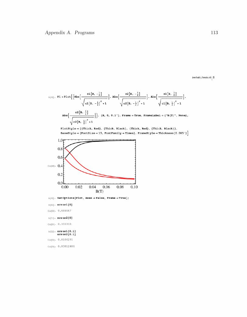
Appendix A. Programs 113

Appendix A. Programs 114

Appendix A. Programs 115

Appendix A. Programs 116

Appendix A. Programs 117
A.2 Inclusion of the quadrupole part for Sr
This program is similar to the one in Appendix A.1, but it includes the quadrupole
part of the Zeeman interaction and is thus suitable for 87Sr. It was thus used to
numerically calculate the spectrum for 87Yb in a magnetic field and the fidelity for
the cooling scheme described in Chapter 3

Appendix A. Programs 118

Appendix A. Programs 119

Appendix A. Programs 120

Appendix A. Programs 121

Appendix A. Programs 122

Appendix A. Programs 123

Appendix A. Programs 124
A.3 Calculation of the multichannel Hamiltonian
This Mathematica 6 program was used to determine the full multichannel Hamil-
tonian from the transformations between the different bases described in Chapter
4. Furthermore, it was used to find the adiabatic potentials and the linewidthma-
trix from the same chapter. The resulting, block diagonal Hamiltonian was then
exported into a fortran Code based on a code by E. Tiesinga and P. Julienne from
NIST which used the DVR method described in Section 4.2.2 to yield the multichan-
nel wave functions.
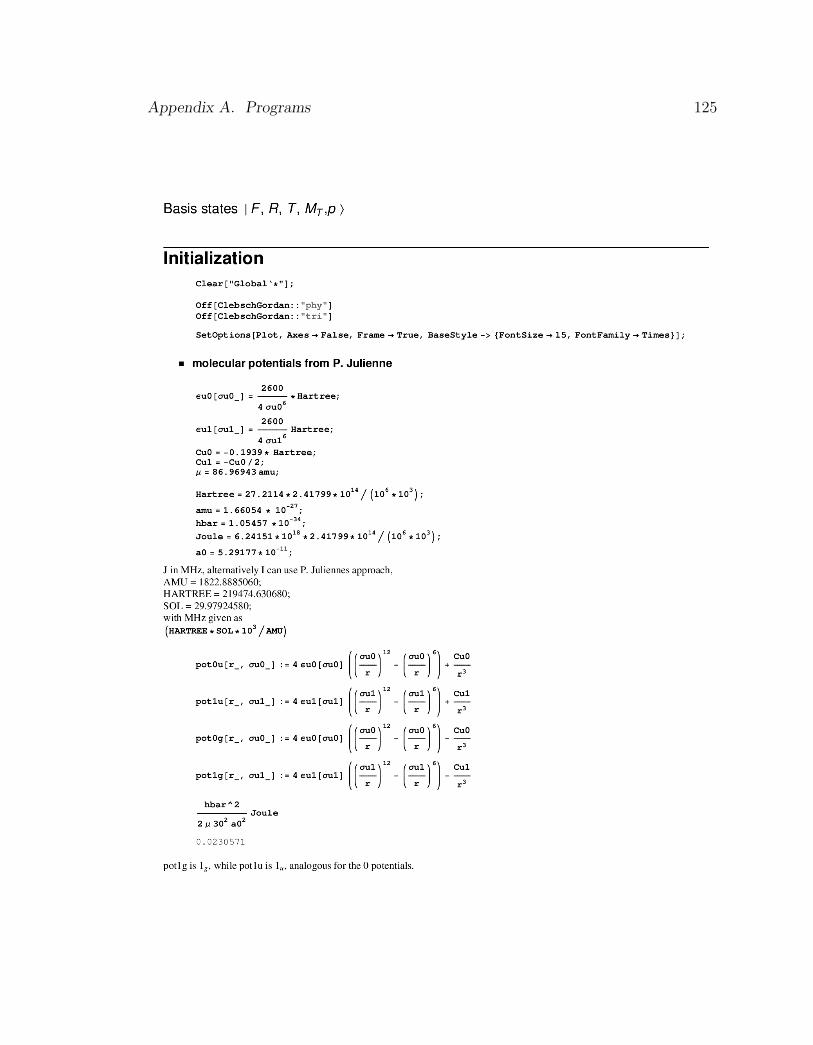
Appendix A. Programs 125

Appendix A. Programs 126

Appendix A. Programs 127

Appendix A. Programs 128

Appendix A. Programs 129

Appendix A. Programs 130

Appendix A. Programs 131

Appendix A. Programs 132

Appendix A. Programs 133
Appendix A. Programs 134

Appendix A. Programs 135

Appendix A. Programs 136

Appendix A. Programs 137

Appendix A. Programs 138
A.4 Determination of the optically induced scat-
tering length
This program first determines the Condon factors and linewidths from the multi-
channel wave functions calculated with fortran and the uses these to calculate the
real and imaginary parts of the scattering length optically induced via the Feshbach
resonance.

Appendix A. Programs 139

Appendix A. Programs 140

Appendix A. Programs 141

Appendix A. Programs 142

Appendix A. Programs 143

Appendix A. Programs 144

Appendix A. Programs 145

Appendix A. Programs 146

Appendix A. Programs 147

Appendix A. Programs 148

149
References
[1] M. M. Boyd. High Precision Spectroscopy of Strontium in an Optical Lattice:Towards a New Standard for Frequency and Time. PhD thesis, University ofColorado, 2007.
[2] S. A. Diddams, J. C. Bergquist, S. R. Jefferts, and C. W. Oates. Standards oftime and frequency at the outset of the 21st century. Science, 306:1318, 2004.
[3] Steven Chu. Nobel lecture: The manipulation of neutral particles. Rev. Mod.Phys., 70(3):685–706, Jul 1998.
[4] Claude N. Cohen-Tannoudji. Nobel lecture: Manipulating atoms with photons.Rev. Mod. Phys., 70(3):707–719, Jul 1998.
[5] William D. Phillips. Nobel lecture: Laser cooling and trapping of neutral atoms.Rev. Mod. Phys., 70(3):721–741, Jul 1998.
[6] Michael A. Nielsen and Isaac L. Chuang. Quantum Computation and QuantumInformation. Cambridge University Press, 2000.
[7] Sergey G. Porsev, Andrei Derevianko, and E. N. Fortson. Possibility of anoptical clock using the 61s0 → 63p0 transition in 171,173yb atoms held in anoptical lattice. Phys. Rev. A, 69(021403(R)):021403 R, February 2004.
[8] Martin M. Boyd, Andrew D. Ludlow, Sebastian Blatt, Seth M. Foreman, Tet-suya Ido, Tanya Zelevinsky, and Jun Ye. 87sr lattice clock with inaccuracy below10−15. Phys. Rev. Lett., 98(8):083002, 2007.
[9] Ivan H. Deutsch and Poul S. Jessen. Quantum-state control in optical lattices.Phys. Rev. A, 57(3):1972–1986, Mar 1998.
[10] Gavin K. Brennen, Carlton M. Caves, Poul S. Jessen, and Ivan H. Deutsch.Quantum logic gates in optical lattices. Phys. Rev. Lett., 82(5):1060, February1999.

References 150
[11] Gavin K. Brennen and Jamie E. Williams. Entanglement dynamics in one-dimensional quantum cellular automata. Phys. Rev. A, 68:042311, October2003.
[12] T. Calarco, U. Dorner, P. S. Julienne, C. J. Williams, and P. Zoller. Quan-tum computations with atoms in optical lattices: Marker qubits and molecularinteractions. Phys. Rev. A, 70(1):012306, Jul 2004.
[13] David Hayes, Paul S. Julienne, and Ivan H. Deutsch. Quantum logic via theexchange blockade in ultracold collisions. Phys. Rev. Lett., 98(7):070501, 2007.
[14] J. Sebby-Strabley, M. Anderlini, P. S. Jessen, and J. V. Porto. Lattice of doublewells for manipulating pairs of cold atoms. Phys. Rev. A, 73(3):033605, 2006.
[15] Immanuel Bloch, Jean Dalibard, and Wilhelm Zwerger. Many-body physicswith ultracold gases. Rev. Mod. Phys., 80(3):885, 2008.
[16] D. Jaksch, C. Bruder, J. I. Cirac, C. W. Gardiner, and Peter Zoller. Coldbosonic atoms in optical lattices. Phys. Rev. Lett., 81(15):3108, October 1998.
[17] W. Hofstetter, J. I. Cirac, P. Zoller, E. Demler, and M. D. Lukin. High-temperature superfluidity of fermionic atoms in optical lattices. Phys. Rev.Lett., 89:220407, November 2002.
[18] D. Jaksch, H.-J. Briegel, J. I. Cirac, C. W. Gardiner, and P. Zoller. Entangle-ment of atoms via cold controlled collisions. Phys. Rev. Lett., 82(9):1975, March1999.
[19] Takeshi Fukuhara, Seiji Sugawa, Masahito Sugimoto, Shintaro Taie, and YoshiroTakahashi. Mott insulator of ultracold alkaline-earth-metal-like atoms. Phys.Rev. A, 79(4):041604, 2009.
[20] Robert Raussendorf. Quantum cellular automaton for universal quantum com-putation. Phys. Rev. A, 72(2):022301, 2005.
[21] R. Raussendorf, J. Harrington, and K. Goyal. A fault-tolerant one-way quantumcomputer. Annals of Physics, 321,:2242, 2006.
[22] Andrew J. Daley, Martin M. Boyd, Jun Ye, and Peter Zoller. Quantum com-puting with alkaline-earth-metal atoms. Phys. Rev. Lett., 101(17):170504, 2008.
[23] L. M. K. Vandersypen and I. L. Chuang. Nmr techniques for quantum controland computation. Rev. Mod. Phys., 76(4):1037–1069, Jan 2005.
[24] Martin M. Boyd, Tanya Zelevinsky, Andrew D. Ludlow, Sebastian Blatt,Thomas Zanon-Willette, Seth M. Foreman, and Jun Ye. Nuclear spin effectsin optical lattice clocks. Phys. Rev. A, 76(2):022510, 2007.

References 151
[25] Z. W. Barber, C. W. Hoyt, C. W. Oates, L. Hollberg, A. V. Taichenachev, andV. I. Yudin. Direct excitation of the forbidden clock transition in neutral 174ybatoms confined to an optical lattice. Phys. Rev. Lett., 96(8):083002, 2006.
[26] Robin Santra, Ennio Arimondo, Tetsuya Ido, Chris H. Greene, and Jun Ye.High-accuracy optical clock via three-level coherence in neutral bosonic 88sr.Phys. Rev. A, 95(173002):173002, May 2005.
[27] Rene Stock, Andrew Silberfarb, Eric L. Bolda, and Ivan H. Deutsch. Generalizedpseudo-potentials for higher partial wave scattering. Phys. Rev. Lett., 94:023202,January 2005.
[28] Rene Stock. Trap-induced resonances in controlled atomic collisions for quantuminformation processing. PhD thesis, University of New Mexico, 2005.
[29] Iris Reichenbach, Andrew Silberfarb, Rene Stock, and Ivan H. Deutsch. Quasi-hermitian pseudopotential for higher partial wave scattering. Phys. Rev. A,74(4):042724, 2006.
[30] Iris Reichenbach and Ivan H. Deutsch. Sideband cooling while preserving co-herences in the nuclear spin state in group-ii-like atoms. Phys. Rev. Lett.,99(12):123001, 2007.
[31] John R. Taylor. Scattering Theory: The Quantum Theory of NonrelativisticCollisions. John Wiley & Sons, Inc., New York, 1972.
[32] Keith Burnett, Paul S. Julienne, Paul D. Lett, Eite Tiesinga, and Carl J.Williams. Quantum encounters of the cold kind. Nature Insight - Ultracoldmatter, 416(6877):225–232, March 2002.
[33] Enrico Fermi. Sul moto dei neutroni nelle sostanze idrogenate. La Ricera Sci-entifica, Serie II, Anno VII, II:13–52, 1936.
[34] Eric L. Bolda, Eite Tiesinga, and P. S. Julienne. Effective-scattering-lengthmodel of ultracold atomic collisions and feshbach resonances in tight harmonictraps. Phys. Rev. A, 66:013403, July 2002.
[35] Cheng Chin, Rudolf Grimm, Paul Julienne, and Eite Tiesinga. Feshbach reso-nances in ultracold gases. 2008.
[36] Keith Burnett, Paul S. Julienne, Paul D. Lett, Eite Tiesinga, and Carl Williams.Quantum encounters of the cold kind. Nature Insight - Ultracold matter,416(6877):225–232, March 2002.

References 152
[37] Rene Stock, Ivan H. Deutsch, and Eric L. Bolda. Quantum state control viatrap-induced shape resonance in ultracold atomic collisions. Phys. Rev. Lett.,91:183201, October 2003.
[38] Marco Anderlini, Patricia J. Lee, Benjamin L. Brown, Jennifer Sebby-Strabley,William D. Phillips, and J. V. Porto. Controlled exchange interaction betweenpairs of neutral atoms in an optical lattice. Nature, 448:452–456, 2007.
[39] Kevin M. Jones, Eite Tiesinga, Paul D. Lett, and Paul S. Julienne. Ultracoldphotoassociation spectroscopy: Long-range molecules and atomic scattering.Rev. Mod. Phys., 78(2):483, 2006.
[40] Paul S. Julienne. Notes on photoassociation of yb and sr.
[41] B. H. Bransden and C. J. Joachain. Physics of Atoms and Molecules. PearsonEducation Limited, second edition, 2003.
[42] Richard N. Zare. Angular Momentum: Understanding Spatial Aspects in Chem-istry and Physics. John Wiley and Sons, 1988.
[43] D. M. Brink and G. R. Satchler. Angular Momentum. Oxford University Press,Oxford, second edition, 1986.
[44] Reginaldo Napolitano, John Weiner, and Paul S. Julienne. Theory of opti-cal suppression of ultracold-collision rates by polarized light. Phys. Rev. A,55(2):1191–1207, Feb 1997.
[45] D. A. Varshalovich, A. N. Moskalev, and V. K. Khersonskii. Quantum Theoryof Angular Momentum. World Scientific Publishing Co., 1988.
[46] M. D. Barrett, B. DeMarco, T. Schaetz, V. Meyer, D. Leibfried, J. Britton,J. Chiaverini, W. M. Itano, B. Jelenkovic, J. D. Jost, C. Langer, T. Rosenband,and D. J. Wineland. Sympathetic cooling of 9be+ and 24mg+ for quantumlogic. Phys. Rev. A, 68(4):042302, Oct 2003.
[47] A. J. Daley, P. O. Fedichev, and P. Zoller. Single-atom cooling by superuidimmersion: A nondestructive method for qubits. Phys. Rev. A, 69(4):022306,February 2004.
[48] F. Diedrich, J. C. Berquist, Wayne M. Itano, D. J. Wineland, F. Diedrich, J. C.Bergquist, Wayne M. Itano, and D. J. Wineland. Laser cooling to the zero-pointenergy of motion. Phys. Rev. Lett., 62(4):403–406, Jan 1989.
[49] Masao Takamoto, Feng-Lei Hong, Ryoichi Higashi, and Hidetoshi Katori. Anoptical lattice clock. Nature, 435:321, 2005.

References 153
[50] Andrew D. Ludlow, Martin M. Boyd, Tanya Zelevinsky, Seth M. Foreman, Se-bastian Blatt, Mark Notcutt, Tetsuya Ido, and Jun Ye. Systematic study of the87sr clock transition in an optical lattice. Phys. Rev. Lett., 96(3):033003, 2006.
[51] C. W. Hoyt, Z. W. Barber, C. W. Oates, T. M. Fortier, S. A. Diddams, andL. Hollberg. Observation and absolute frequency measurements of the 1s0 −3
p0 optical clock transition in ytterbium. Phys. Rev. Lett., 95(083003):083003,August 2005.
[52] Martin M. Boyd, Tanya Zelevinsky, Andrew D. Ludlow, Seth M. Foreman, Se-bastian Blatt, Tetsuya Ido, and Jun Ye. Optical atomic coherence at the 1-second time scale. Science, 314(5804):1430–1433, 2006.
[53] Christopher J. Foot. Atomic Physics. Oxford University Press, Oxford, 2004.
[54] D. J. Wineland and Wayne M. Itano. Laser cooling of atoms. Phys. Rev. A,20(4):1521–1540, Oct 1979.
[55] D. Leibfried, R. Blatt, C. Monroe, and D. Wineland. Quantum dynamics ofsingle trapped ions. Rev. Mod. Phys., 75(1):281–324, Mar 2003.
[56] C. Monroe, D. M. Meekhof, B. E. King, S. R. Jefferts, W. M. Itano, D. J.Wineland, and P. Gould. Resolved-sideband raman cooling of a bound atom tothe 3d zero-point energy. Phys. Rev. Lett., 75(22):4011–4014, Nov 1995.
[57] H. Perrin, A. Kuhn, I. Bouchoule, and C. Salomon. Sideband cooling of neutralatoms in a far-detuned optical lattice. EPL (Europhysics Letters), 42(4):395–400, 1998.
[58] Ivan H. Deutsch. Lecture notes on quantum optics.http://info.phys.unm.edu/ deutschgroup/Classes/Phys566F08/index.htm.
[59] Marlan O. Scully and Mohammad S. Zubairy. Quantum Optics. CambridgeUniversity Press, 1997.
[60] U. Sterr, C. Degenhardt, H. Stoehr, Ch. Lisdat, H. Schnatz, J. Helmcke,F. Riehle, G. Wilpers, Ch. Oates, and L. Hollberg. The optical calcium fre-quency standards of ptb and nist. Comptes Rendus Physique, 5(8):845 – 855,2004. Fundamental metrology.
[61] E. Anne Curtis, Christopher W. Oates, and Leo Hollberg. Quenched narrow-linesecond- and third-stage laser cooling of 40 ca. J. Opt. Soc. Am. B, 20(5):977–984, 2003.
[62] Wayne M. Itano, D. J. Heinzen, J. J. Bollinger, and D. J. Wineland. Quantumzeno effect. Phys. Rev. A, 41(5):2295–2300, Mar 1990.

References 154
[63] R. W Berends and L. Maleki. Hyperfine structure and isotope shifts of transi-tions in neutral and singly ionized ytterbium. J. Opt. Soc. Am. B, 9(8):8, March1992.
[64] H. Jurgen Kluge and Hatto Sauter. Levelcrossing experiments in the first excited1p1 states of the alkaline earths. Z. Phys., 240:295, 1974.
[65] Anders Brusch, Rodolphe Le Targat, Xavier Baillard, Mathilde Fouche, andPierre Lemonde. Hyperpolarizability effects in a sr optical lattice clock. Phys.Rev. Lett., 96(10):103003, 2006.
[66] A. V. Gorshkov, A. M. Rey, A. J. Daley, M. M. Boyd, J. Ye, P. Zoller, andM. D. Lukin. Alkaline-earth-metal atoms as few-qubit quantum registers. Phys.Rev. Lett., 102(11):110503, 2009.
[67] Herman Feshbach. Unified theory of nuclear reactions. Annals of Physics,5(4):357, 1958.
[68] U. Fano. Effects of configuration interaction on intensities and phase shifts.Phys. Rev., 124(6):1866–1878, Dec 1961.
[69] Cindy A. Regal, Christopher Ticknor, John L. Bohn, and Deborah S. Jin. Cre-ation of ultracold molecules from a fermi gas of atoms. Nature, 424(6944):47,2003.
[70] K.-K. Ni, S. Ospelkaus, M. H. G. de Miranda, A. Pe’er, B. Neyenhuis, J. J.Zirbel, S. Kotochigova, P. S. Julienne, D. S. Jin, and J. Ye. A high phase-space-density gas of polar molecules. Science, 322(5899):231–235, 2008.
[71] D. DeMille. Quantum computation with trapped polar molecules. Phys. Rev.Lett., 88(6):067901, Jan 2002.
[72] T. Bourdel, L. Khaykovich, J. Cubizolles, J. Zhang, F. Chevy, M. Teichmann,L. Tarruell, S. J. J. M. F. Kokkelmans, and C. Salomon. Experimental studyof the bec-bcs crossover region in lithium 6. Phys. Rev. Lett., 93(5):050401, Jul2004.
[73] Stefano Giorgini, Lev P. Pitaevskii, and Sandro Stringari. Theory of ultracoldatomic fermi gases. Rev. Mod. Phys., 80(4):1215, 2008.
[74] P. O. Fedichev, Yu. Kagan, G. V. Shlyapnikov, and J. T. M. Walraven. Influenceof nearly resonant light on the scattering length in low-temperature atomic gases.Phys. Rev. Lett., 77(14):2913–2916, Sep 1996.
[75] John L. Bohn and P. S. Julienne. Prospects for influencing scattering lengthswith far-off-resonant light. Phys. Rev. A, 56(2):1486–1491, Aug 1997.

References 155
[76] F. K. Fatemi, K. M. Jones, and P. D. Lett. Observation of optically inducedfeshbach resonances in collisions of cold atoms. Phys. Rev. Lett., 85(21):4462–4465, Nov 2000.
[77] M. Theis, G. Thalhammer, K. Winkler, M. Hellwig, G. Ruff, R. Grimm, andJ. Hecker Denschlag. Tuning the scattering length with an optically inducedfeshbach resonance. Phys. Rev. Lett., 93(12):123001, Sep 2004.
[78] Gregor Thalhammer, Matthias Theis, Klaus Winkler, Rudolf Grimm, and Jo-hannes Hecker Denschlag. Inducing an optical feshbach resonance via stimulatedraman coupling. Phys. Rev. A, 71(3):033403, 2005.
[79] R. Ciury lo, E. Tiesinga, and P. S. Julienne. Optical tuning of the scatteringlength of cold alkaline-earth-metal atoms. Phys. Rev. A, 71(3):030701, Mar2005.
[80] K. Enomoto, K. Kasa, M. Kitagawa, and Y. Takahashi. Optical feshbach reso-nance using the intercombination transition. Phys. Rev. Lett., 101(20):203201,2008.
[81] Katsunari Enomoto, Masaaki Kitagawa, Satoshi Tojo, and Yoshiro Takahashi.Hyperfine-structure-induced purely long-range molecules. Phys. Rev. Lett.,100(12):123001, 2008.
[82] T. Zelevinsky, M. M. Boyd, A. D. Ludlow, T. Ido, J. Ye, R. Ciury lo, P. Naidon,and P. S. Julienne. Narrow line photoassociation in an optical lattice. Phys.Rev. Lett., 96(20):203201, 2006.
[83] Y. N. Martinez de Escobar, P. G. Mickelson, M. Yan, and T. C. Killian. Tuningthe elastic collision cross section with an intercombination-line optical feshbachresonance. unpublished.
[84] John L. Bohn and P. S. Julienne. Semianalytic theory of laser-assisted resonantcold collisions. Phys. Rev. A, 60(1):414–425, Jul 1999.
[85] Eite Tiesinga, Kevin M. Jones, Paul D. Lett, Udo Volz, Carl J. Williams, andPaul S. Julienne. Measurement and modeling of hyperfine- and rotation-inducedstate mixing in large weakly bound sodium dimers. Phys. Rev. A, 71(5):052703,2005.
[86] Bo Gao. Solutions of the schrodinger equation for an attractive 1/r6 potential.Phys. Rev. A, 58(3):1728–1734, Sep 1998.
[87] Masaaki Kitagawa, Katsunari Enomoto, Kentaro Kasa, Yoshiro Takahashi, Ro-man Ciury lo, Pascal Naidon, and Paul S. Julienne. Two-color photoassociation

References 156
spectroscopy of ytterbium atoms and the precise determinations of s-wave scat-tering lengths. Phys. Rev. A, 77(1):012719, 2008.
[88] J. C. Light, I. P. Hamilton, and J. V. Lill. Generalized discrete variable approx-imation in quantum mechanics. The Journal of Chemical Physics, 82(3):1400–1409, 1985.
[89] Daniel T. Colbert and William H. Miller. A novel discrete variable representationfor quantum mechanical reactive scattering via the s-matrix kohn method. J.Chem. Phys., 96(3):1982–1991, 1992.
[90] Rene Stock and Ivan H. Deutsch. Trap-induced resonances in controlled colli-sions of cesium atoms. Phys. Rev. A, 73:032701, March 2006.