1

Transportation Research Record: Journal of the Transportation Research Board, No. 2546, Transportation Research Board, Washington, D.C., 2016, pp. 1–8.DOI: 10.3141/2546-01

To minimize costs, railways carefully match route infrastructure invest-ment to projected traffic levels. Under structured operations according to a rigid timetable, the optimal amount of infrastructure for a given traffic volume can be determined with various models. However, North Ameri-can railways use flexible operations for which planned train departure times can vary. Schedule flexibility increases the number of possible meet locations on a single track, which can lead to a combination of increased delays and infrastructure investment. When industry practitioners plan rail line capacity for flexible operations, they rarely optimize schedule flexibility and infrastructure investment simultaneously for a given level of service. To increase knowledge of the relationship between these factors, the research reported in this paper simulated operations on two representative single-track routes with rail traffic controller software. A baseline minimum-delay schedule was developed for each route under an initial infrastructure. The experiment design introduced schedule flexibility and infrastructure expansion to examine the interaction between these factors and train delay response. The results suggested that, for a given infrastructure configuration, an immediate increase in train delay occurred with small amounts of schedule flexibility. After this increase, routes became insensitive to further increases in schedule flexibility. Similarly, to maintain a level of service required substantial infrastructure investment for small amounts of schedule flexibility.

North American railroads are among the most capital-intensive of industries. In recent years, freight railroads in the United States have invested 19% of their revenues in capital expenditures. This rate of investment is more than six times higher than that of the typical U.S. manufacturer (1). In addition to initial investments for construction of passing sidings, second mainline tracks, and terminal facilities, railroads must fund the ongoing costs of inspection and maintenance of their fixed track infrastructure. These expenditures amount to bil-lions of dollars each year (2). Although some components of the track structure, such as rail, can be salvaged for reuse, most railroad infrastructure capital and maintenance expenses are nonfungible and with limited liquidity. Thus, to maintain a solid financial position, railroads must carefully match their track infrastructure layout to planned levels of traffic. Although inadequate track infrastructure creates congestion and delay that limits revenue potential, excess

infrastructure can unnecessarily consume railroad capital, inspection, and maintenance resources.

Numerous capacity evaluation tools are available to industry practitioners to assess the amount of infrastructure investment in the passing sidings and double track required for a given traffic volume. Simple analytical models, such as the return-grid method on single track, can quickly relate siding spacing and average train speed to a theoretical maximum traffic volume (3). However, to match the performance of this approach, all trains on a route must travel at the same average speed and depart the end terminals at precise intervals. Previous research has documented how different train operating speeds, or “speed heterogeneity,” can interrupt this operating pattern and increase delay while they decrease the capacity of the line to handle traffic (4–6). Under these conditions, the capacity of the line is defined by the rail traffic volume that corresponds to an average train delay threshold set to maintain a required level of service (7).

Optimization models have been developed to determine the pattern of passing sidings and double-track segments that minimize train delay on routes with a mixture of different passenger and freight trains (8, 9). Although these models consider trains that operate at different maximum speeds, they optimize the infrastructure on the basis of a precise pattern of train departures from end terminals. The optimal infrastructure plan generated by these models becomes specific to a certain train schedule. A change in the departure time or average speed of one or more trains can lead to a different optimal result.

Structured VerSuS Flexible OperatiOnS

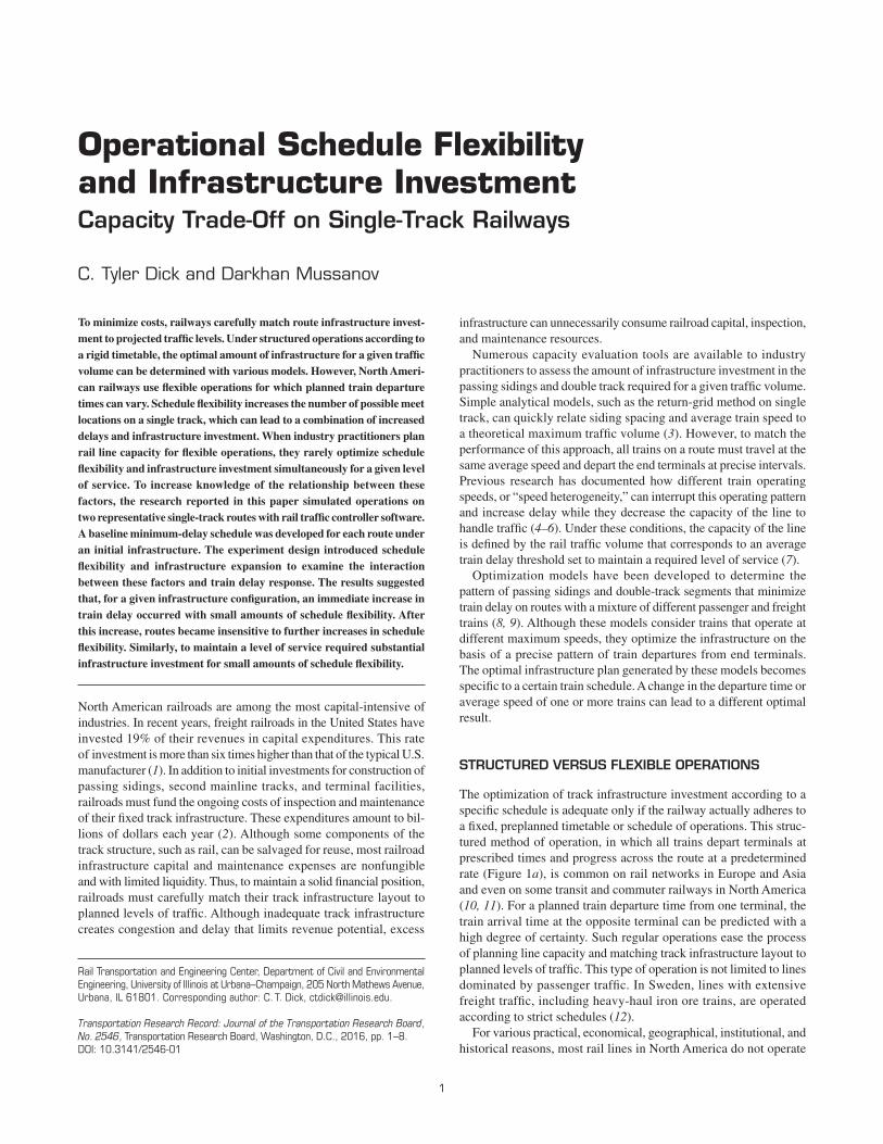
The optimization of track infrastructure investment according to a specific schedule is adequate only if the railway actually adheres to a fixed, preplanned timetable or schedule of operations. This struc-tured method of operation, in which all trains depart terminals at prescribed times and progress across the route at a predetermined rate (Figure 1a), is common on rail networks in Europe and Asia and even on some transit and commuter railways in North America (10, 11). For a planned train departure time from one terminal, the train arrival time at the opposite terminal can be predicted with a high degree of certainty. Such regular operations ease the process of planning line capacity and matching track infrastructure layout to planned levels of traffic. This type of operation is not limited to lines dominated by passenger traffic. In Sweden, lines with extensive freight traffic, including heavy-haul iron ore trains, are operated according to strict schedules (12).

For various practical, economical, geographical, institutional, and historical reasons, most rail lines in North America do not operate

Operational Schedule Flexibility and Infrastructure Investmentcapacity trade-Off on Single-track railways

C. Tyler Dick and Darkhan Mussanov

Rail Transportation and Engineering Center, Department of Civil and Environmental Engineering, University of Illinois at Urbana–Champaign, 205 North Mathews Avenue, Urbana, IL 61801. Corresponding author: C. T. Dick, ctdick@illinois.edu.

2 Transportation Research Record 2546

according to a precise fixed timetable. Instead, these lines exhibit a flexible method of operation. Although the same general pattern of trains may operate on a given day from week to week, a specific train may depart a terminal over a range of times (Figure 1b) and progress across the route at varying rates (Figure 1c). Variation in running time may result from a combination of the unique acceleration and braking performance of each individual train and the exact pattern of meets and passes encountered on a particular trip. When the effects of depar-ture time variation and variability in running time are combined to offer full schedule flexibility, the arrival time of a particular train at the end terminal (or intermediate locations along the route) is subject to large uncertainty relative to the case of a fixed timetable. The amount of schedule flexibility for different train types will not be the same. To satisfy customer service needs, passenger trains and priority inter-modal trains are likely to have relatively fixed departure and running times (i.e., little schedule flexibility). A bulk unit train with a rather predictable train consist is likely to have a relatively fixed running time but may exhibit much variation in departure time according to shipper production and delivery schedules. Manifest trains may have relatively fixed departure times from classification yards but are likely to experience variations in running time as the result of fluctuations in daily train makeup and meets with priority trains.

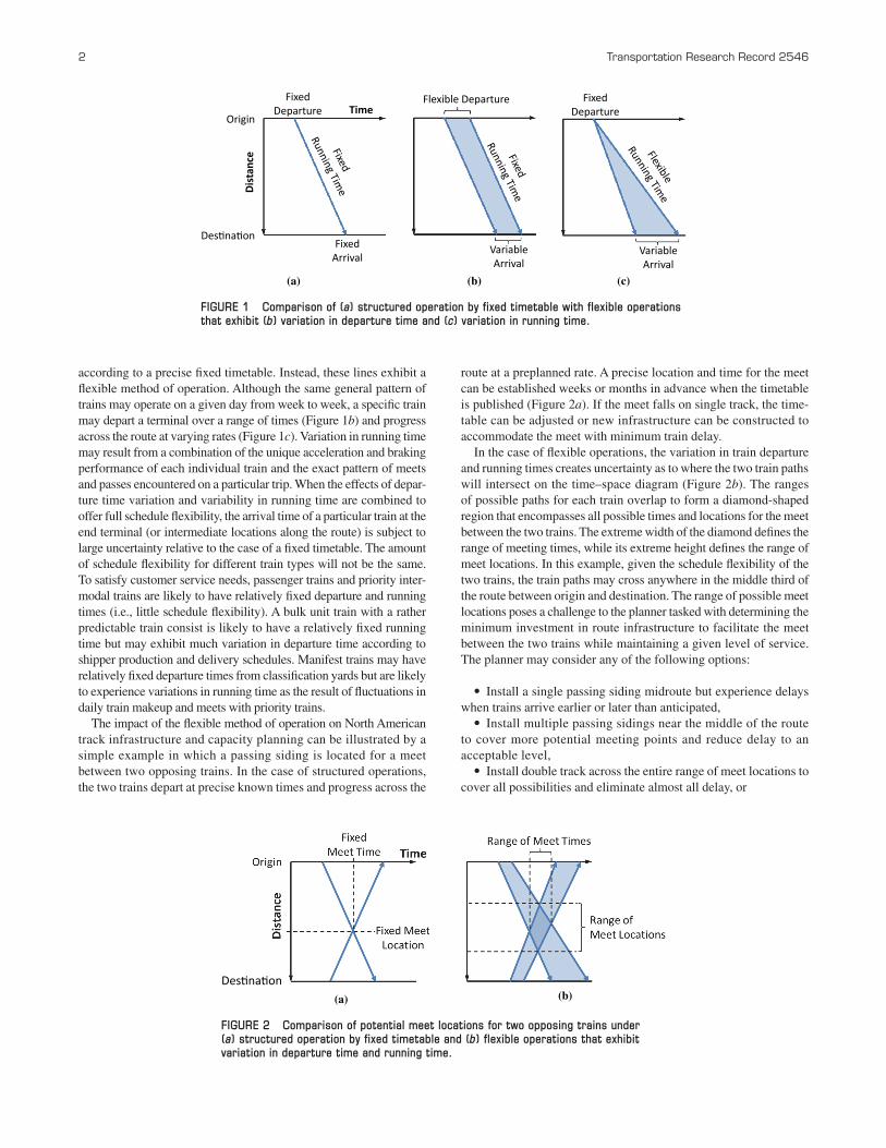
The impact of the flexible method of operation on North American track infrastructure and capacity planning can be illustrated by a simple example in which a passing siding is located for a meet between two opposing trains. In the case of structured operations, the two trains depart at precise known times and progress across the

route at a preplanned rate. A precise location and time for the meet can be established weeks or months in advance when the timetable is published (Figure 2a). If the meet falls on single track, the time-table can be adjusted or new infrastructure can be constructed to accommodate the meet with minimum train delay.

In the case of flexible operations, the variation in train departure and running times creates uncertainty as to where the two train paths will intersect on the time–space diagram (Figure 2b). The ranges of possible paths for each train overlap to form a diamond-shaped region that encompasses all possible times and locations for the meet between the two trains. The extreme width of the diamond defines the range of meeting times, while its extreme height defines the range of meet locations. In this example, given the schedule flexibility of the two trains, the train paths may cross anywhere in the middle third of the route between origin and destination. The range of possible meet locations poses a challenge to the planner tasked with determining the minimum investment in route infrastructure to facilitate the meet between the two trains while maintaining a given level of service. The planner may consider any of the following options:

• Install a single passing siding midroute but experience delays when trains arrive earlier or later than anticipated,• Install multiple passing sidings near the middle of the route

to cover more potential meeting points and reduce delay to an acceptable level,• Install double track across the entire range of meet locations to

cover all possibilities and eliminate almost all delay, or

(b) (c)

Fixed

Running Time

Flexible Departure

VariableArrival

Flexible

Running Time

FixedDeparture

VariableArrival

(a)

Origin

Destination

Fixed

Running Time

FixedDeparture

FixedArrival

Dist

ance

Time

FIGURE 1 Comparison of (a) structured operation by fixed timetable with flexible operations that exhibit (b) variation in departure time and (c) variation in running time.

(a) (b)Destination

FIGURE 2 Comparison of potential meet locations for two opposing trains under (a) structured operation by fixed timetable and (b) flexible operations that exhibit variation in departure time and running time.

Dick and Mussanov 3

• Reduce schedule flexibility to narrow the range of meet loca-tions until a single passing siding can cover all possible meets with acceptable delay.

These options illustrate a trade-off between schedule flexibility, investment in route infrastructure, and level of service, which was the subject of the research reported in this paper.

reSearch QueStiOnS

It is common for railroad practitioners in North America to use simulation or parametric models to plan route infrastructure under flexible operations. Simulation models account for schedule flex-ibility by replicating traffic and infrastructure simulations for different randomized train departure patterns. Although such an approach makes it possible to assess the performance of an infrastructure investment under a range of scheduling assumptions, there is no guarantee that all possible traffic combinations will be considered and that a true optimal solution will be found.

Parametric models do not consider schedule flexibility directly as an input but account for its effects in the conversion of theoretical line capacity to practical line capacity. In most parametric models of rail line capacity, there is no way to adjust the level of schedule flex-ibility and observe the response of other variables (e.g., delay, traffic volume, route infrastructure).

Also, a different set of software tools allows railroads to develop optimal manifest and intermodal operating plans with allowance for schedule flexibility on a given track infrastructure. CSX Trans-portation uses a computer-aided routing and scheduling system dedicated to live optimization of routing and scheduling (13). Ping et al. researched intelligent train dispatching methods (14). Lu et al. introduced train performance calculations in the scheduling meth-odology (15). In this manner, industry planning usually focuses on the evaluation of infrastructure investment under a given operating plan or on the development of an operating plan for a given infrastructure. The industry currently lacks tools that can simultaneously optimize route infrastructure and the operating plan in an efficient manner.

To aid practitioners in making decisions on capacity-expansion projects and in developing train plans, the research reported here sought to develop a more fundamental understanding of the rela-tionship between schedule flexibility, infrastructure investment, and level of service on single-track railway lines. Through a better under-standing of this relationship, industry practitioners can make more informed decisions on the combination of schedule flexibility and infrastructure investment to meet business objectives and minimize the overall cost.

To achieve this goal, this paper addresses two research questions:

• For a given route infrastructure layout, what is the level-of-service penalty for the operation of a flexible schedule?• How much extra route infrastructure is required to support a

certain amount of schedule flexibility while a given level of service is maintained?

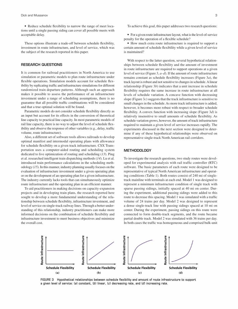
With respect to the latter question, several hypothetical relation-ships between schedule flexibility and the amount of investment in route infrastructure are required to support operations at a given level of service (Figure 3, a–d). If the amount of route infrastructure remains constant as schedule flexibility increases (Figure 3a), the track layout is robust and not sensitive to changes in schedule. A linear relationship (Figure 3b) indicates that a unit increase in schedule flexibility requires the same increase in route infrastructure at all levels of schedule variation. A concave function with decreasing slope (Figure 3c) suggests that the track infrastructure is sensitive to small changes in the schedule. As more track infrastructure is added, however, it becomes more robust with respect to broader schedule flexibility. A convex function with increasing slope (Figure 3d) is relatively insensitive to small amounts of schedule flexibility. As schedule variation grows, however, the amount of track infrastructure required to maintain a given level of service increases rapidly. The experiments discussed in the next section were designed to deter-mine if any of these hypothetical relationships were observed on representative single-track North American rail corridors.

MethOdOlOgy

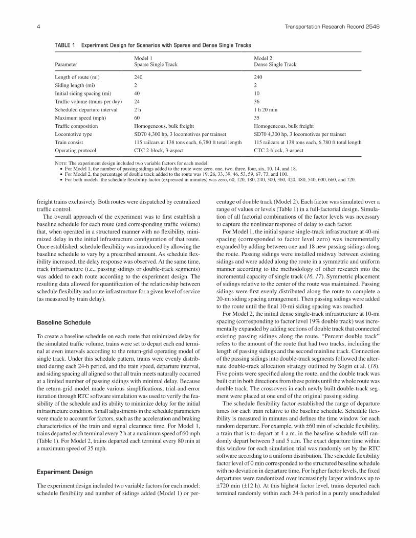
To investigate the research questions, two study routes were devel-oped for experimental analysis with rail traffic controller (RTC) software. The basic parameters of each route were designed to be representative of typical North American infrastructure and operat-ing conditions (Table 1). Both routes consist of 240 mi of single-track mainline with terminals at each end. Model 1 was designed to represent a minimum infrastructure condition of single track with sparse passing sidings, initially spaced at 40 mi on center. Dur-ing the experiment, additional passing sidings were added to this route to decrease this spacing. Model 1 was simulated with a traffic volume of 24 trains per day. Model 2 was designed to represent a dense single-track line with passing sidings spaced at 10 mi on center. During the experiment, passing sidings on this route were connected to form double-track segments, and the route became partial double track. Model 2 was simulated with 36 trains per day. In both cases the traffic was homogeneous and comprised bulk-unit

FIGURE 3 Hypothetical relationships between schedule flexibility and amount of route infrastructure to support a given level of service: (a) constant, (b) linear, (c) decreasing rate, and (d) increasing rate.

(a)

Rout

e In

fras

truc

ture

Schedule Flexibility(c)

Rout

e In

fras

truc

ture

Schedule Flexibility(b)

Rout

e In

fras

truc

ture

Schedule Flexibility(d)

Rout

e In

fras

truc

ture

Schedule Flexibility

4 Transportation Research Record 2546

freight trains exclusively. Both routes were dispatched by centralized traffic control.

The overall approach of the experiment was to first establish a baseline schedule for each route (and corresponding traffic volume) that, when operated in a structured manner with no flexibility, mini-mized delay in the initial infrastructure configuration of that route. Once established, schedule flexibility was introduced by allowing the baseline schedule to vary by a prescribed amount. As schedule flex-ibility increased, the delay response was observed. At the same time, track infrastructure (i.e., passing sidings or double-track segments) was added to each route according to the experiment design. The resulting data allowed for quantification of the relationship between schedule flexibility and route infrastructure for a given level of service (as measured by train delay).

baseline Schedule

To create a baseline schedule on each route that minimized delay for the simulated traffic volume, trains were set to depart each end termi-nal at even intervals according to the return-grid operating model of single track. Under this schedule pattern, trains were evenly distrib-uted during each 24-h period, and the train speed, departure interval, and siding spacing all aligned so that all train meets naturally occurred at a limited number of passing sidings with minimal delay. Because the return-grid model made various simplifications, trial-and-error iteration through RTC software simulation was used to verify the fea-sibility of the schedule and its ability to minimize delay for the initial infrastructure condition. Small adjustments in the schedule parameters were made to account for factors, such as the acceleration and braking characteristics of the train and signal clearance time. For Model 1, trains departed each terminal every 2 h at a maximum speed of 60 mph (Table 1). For Model 2, trains departed each terminal every 80 min at a maximum speed of 35 mph.

experiment design

The experiment design included two variable factors for each model: schedule flexibility and number of sidings added (Model 1) or per-

centage of double track (Model 2). Each factor was simulated over a range of values or levels (Table 1) in a full-factorial design. Simula-tion of all factorial combinations of the factor levels was necessary to capture the nonlinear response of delay to each factor.

For Model 1, the initial sparse single-track infrastructure at 40-mi spacing (corresponded to factor level zero) was incrementally expanded by adding between one and 18 new passing sidings along the route. Passing sidings were installed midway between existing sidings and were added along the route in a symmetric and uniform manner according to the methodology of other research into the incremental capacity of single track (16, 17). Symmetric placement of sidings relative to the center of the route was maintained. Passing sidings were first evenly distributed along the route to complete a 20-mi siding spacing arrangement. Then passing sidings were added to the route until the final 10-mi siding spacing was reached.

For Model 2, the initial dense single-track infrastructure at 10-mi spacing (corresponding to factor level 19% double track) was incre-mentally expanded by adding sections of double track that connected existing passing sidings along the route. “Percent double track” refers to the amount of the route that had two tracks, including the length of passing sidings and the second mainline track. Connection of the passing sidings into double-track segments followed the alter-nate double-track allocation strategy outlined by Sogin et al. (18). Five points were specified along the route, and the double track was built out in both directions from these points until the whole route was double track. The crossovers in each newly built double-track seg-ment were placed at one end of the original passing siding.

The schedule flexibility factor established the range of departure times for each train relative to the baseline schedule. Schedule flex-ibility is measured in minutes and defines the time window for each random departure. For example, with ±60 min of schedule flexibility, a train that is to depart at 4 a.m. in the baseline schedule will ran-domly depart between 3 and 5 a.m. The exact departure time within this window for each simulation trial was randomly set by the RTC software according to a uniform distribution. The schedule flexibility factor level of 0 min corresponded to the structured baseline schedule with no deviation in departure time. For higher factor levels, the fixed departures were randomized over increasingly larger windows up to ±720 min (±12 h). At this highest factor level, trains departed each terminal randomly within each 24-h period in a purely unscheduled

TABLE 1 Experiment Design for Scenarios with Sparse and Dense Single Tracks

ParameterModel 1 Sparse Single Track

Model 2 Dense Single Track

Length of route (mi) 240 240

Siding length (mi) 2 2

Initial siding spacing (mi) 40 10

Traffic volume (trains per day) 24 36

Scheduled departure interval 2 h 1 h 20 min

Maximum speed (mph) 60 35

Traffic composition Homogeneous, bulk freight Homogeneous, bulk freight

Locomotive type SD70 4,300 hp, 3 locomotives per trainset SD70 4,300 hp, 3 locomotives per trainset

Train consist 115 railcars at 138 tons each, 6,780 ft total length 115 railcars at 138 tons each, 6,780 ft total length

Operating protocol CTC 2-block, 3-aspect CTC 2-block, 3-aspect

Note: The experiment design included two variable factors for each model: • For Model 1, the number of passing sidings added to the route were zero, one, two, three, four, six, 10, 14, and 18. • For Model 2, the percentage of double track added to the route was 19, 26, 33, 39, 46, 53, 59, 67, 73, and 100. • For both models, the schedule flexibility factor (expressed in minutes) was zero, 60, 120, 180, 240, 300, 360, 420, 480, 540, 600, 660, and 720.

Dick and Mussanov 5

operation. Through the inclusion of these extremes, a whole spectrum of methods of operation was considered, which ranged from purely structured to extremely flexible.

rtc Simulation

The train-delay response for each experiment scenario was determined through the use of RTC simulation software. RTC is widely used in the rail industry (e.g., by Amtrak, Class I railroads, and consultants) among others. The simulation software closely emulates dispatcher decisions in the guidance of trains along specific routes to resolve meet and pass conflicts. General RTC model inputs include, for example, track layout, signaling, curvature, grades, and train characteristics.

To determine a train-delay response, each unique combination of schedule flexibility and route infrastructure in the experiment design was simulated in RTC for 5 days of rail traffic. To allow for variation in train departure times according to the schedule flexibility factor, each simulation was replicated 10 times to provide 50 days of train operations used to calculate average train delay. Each replication rep-resented a specific departure time set by a uniform distribution over the departure time window. Delay accumulated by individual trains during this 50-day period was averaged and normalized to produce a delay per 100 train-miles response for that element of the experi-

ment design matrix. This average response for a simulation scenario was plotted as a single data point in the results.

reSultS

Schedule Flexibility and train delay

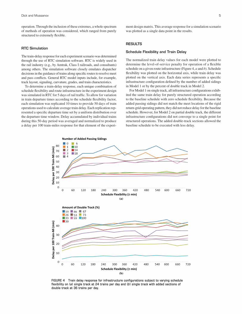
The normalized train delay values for each model were plotted to determine the level-of-service penalty for operation of a flexible schedule on a given route infrastructure (Figure 4, a and b). Schedule flexibility was plotted on the horizontal axis, while train delay was plotted on the vertical axis. Each data series represents a specific infrastructure configuration defined by the number of added sidings in Model 1 or by the percent of double track in Model 2.

For Model 1 on single track, all infrastructure configurations exhib-ited the same train delay for purely structured operation according to the baseline schedule with zero schedule flexibility. Because the added passing sidings did not match the meet locations of the rigid return-grid operating pattern, they did not reduce delay for the baseline schedule. However, for Model 2 on partial double track, the different infrastructure configurations did not converge to a single point for structured operations. The added double-track sections allowed the baseline schedule to be executed with less delay.

(a)

(b)

Del

ay p

er 1

00 T

rain

-Mi (

min

)D

elay

per

100

Tra

in-M

i (m

in)

Schedule Flexibility (± min)

Schedule Flexibility (± min)

Amount of Double Track (%)

Number of Added Passing Sidings

FIGURE 4 Train delay response for infrastructure configurations subject to varying schedule flexibility on (a) single track at 24 trains per day and (b) single track with added sections of double track at 36 trains per day.

6 Transportation Research Record 2546

Both graphs display a concave function with decreasing slope that levels out at high schedule flexibility. The shape of the concave function defines two general ranges of interest: low schedule flex-ibility between 0 and ±120 min (0 and 2 h) of variation and high schedule flexibility from ±120 to ±720 min (2 to 12 h) of variation. In the range of low schedule flexibility for a particular infrastructure condition, train delay was sensitive to small increases in schedule variation. For the initial single-track route in Model 1 with 40-mi siding spacing, a move from structured operations to a flexible sched-ule of ±60 min more than doubled average train delay. This effect was less apparent for the partial double-track route in Model 2. However, the largest increases in delay occurred during the initial deviations from structured operations.

As schedule flexibility increased beyond ±120 min, average train delay values became indifferent to increased variation in the depar-ture schedule. Even in their initial configurations with minimum infrastructure, the single-track routes with 40- and 10-mi siding spac-ing were relatively robust with respect to further increases in schedule flexibility beyond the initial deviations from structured operations.

To explain this result, it was hypothesized that, at low levels of schedule flexibility, train departures fell slightly off the ideal return-grid train paths, which caused meets to be mistimed and led directly to increased train delay. However, at high levels of schedule flex-ibility, trains were shifted far enough from their scheduled departures that they might have fallen closer to the original path of another train and not generated additional delay beyond that created by the initial schedule flexibility.

The point at which a route becomes robust with respect to changes in schedule flexibility is likely to be of interest to railroad planners in charge of developing an operating plan for a given route infrastructure. The implication is that routes that currently operate with several hours of schedule flexibility do not experience delay (and level of service) penalties if the schedule becomes more flexible or service disrup-tions introduce additional variation in train departures. Conversely, routes that currently operate under a strict schedule may face severely increased delay and degraded service as a result of small variations in train departures. From a different perspective, for a purely flexible operation to improve its level of service, schedule flexibility must be decreased below ±60 min to highly structured operations. Little ben-efit is gained from decreases from high to medium levels in schedule flexibility.

Delay response also is a function of traffic volume. The Model 1 route with 18 added passing sidings had the same route infrastructure as it did under the initial condition for Model 2 with 10-mi siding spacing (19% double track). At 24 trains per day (Model 1), the 18-siding configuration was insensitive to schedule flexibility, while at 36 trains per day (Model 2), the same 19% double-track case exhibited sensitivity to schedule variation. As capacity use increased, so did the effect of schedule variation on delay.

As Figure 4, a and b, also shows, configurations with more route infrastructure in general were less sensitive to schedule flexibility. This finding can be observed in the slopes of the initial portion of the delay curve between 0 and 120 min of schedule flexibility, and in the fluctuations of each delay curve at higher levels of schedule flexibility.

route infrastructure and Schedule Flexibility

Through an examination of the combinations of schedule flexibility and infrastructure configurations that corresponded to a given aver-age train delay (level of service) in Figure 4, a and b, the data could

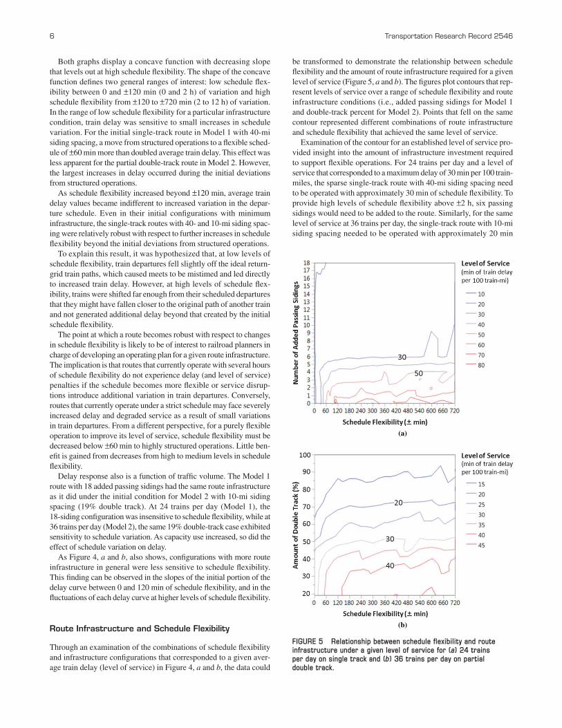
be transformed to demonstrate the relationship between schedule flexibility and the amount of route infrastructure required for a given level of service (Figure 5, a and b). The figures plot contours that rep-resent levels of service over a range of schedule flexibility and route infrastructure conditions (i.e., added passing sidings for Model 1 and double-track percent for Model 2). Points that fell on the same contour represented different combinations of route infrastructure and schedule flexibility that achieved the same level of service.

Examination of the contour for an established level of service pro-vided insight into the amount of infrastructure investment required to support flexible operations. For 24 trains per day and a level of service that corresponded to a maximum delay of 30 min per 100 train-miles, the sparse single-track route with 40-mi siding spacing need to be operated with approximately 30 min of schedule flexibility. To provide high levels of schedule flexibility above ±2 h, six passing sidings would need to be added to the route. Similarly, for the same level of service at 36 trains per day, the single-track route with 10-mi siding spacing needed to be operated with approximately 20 min

(a)

(b)

FIGURE 5 Relationship between schedule flexibility and route infrastructure under a given level of service for (a) 24 trains per day on single track and (b) 36 trains per day on partial double track.

Dick and Mussanov 7

of schedule flexibility. To provide high levels of schedule flexibil-ity above ±2 h, the route infrastructure would need to be expanded until 50% of the line was double track. In both cases, a sizeable investment in infrastructure would be necessary solely to provide schedule flexibility with no increase in traffic volume or improvement in train delay.

Models 1 and 2 suggested a concave relationship between sched-ule flexibility and route infrastructure with a decreasing slope. The amount of track infrastructure required to maintain a level of service was highly sensitive to initial increases in schedule flexibility. How-ever, the infrastructure quickly became robust with respect to large values of schedule flexibility.

Model 1 exhibited a particularly sharp transition between struc-tured and flexible operation (Figure 5a). Operation of a structured schedule with the minimum number of passing sidings is a fragile condition. Small increases in schedule flexibility require the addi-tion of multiple passing sidings to maintain the desired level of ser-vice. At a certain level, with the installation of one passing siding, the condition of the route will change from fragile to robust and insensitive to further increases in schedule flexibility. With 30 min of delay, this transition took place after the sixth passing siding was added. This point was the one at which all 40-mi gaps between pass-ing sidings were eliminated, and the route had sidings spaced evenly at 20 mi on center. Model 2 appeared to involve a less severe transition (Figure 5b), which might have been the result of the relative scales of the plots. The partial double-track route exhibited the same trend (i.e., grew robust in response to schedule variation once an initial infrastructure investment was made).

From the perspective of an infrastructure and capacity planner, these results suggest that, given the desired level of service, little investment in route infrastructure can be saved unless schedule flex-ibility is reduced below ±60 to ±120 min of variation. However, structured operation on minimal infrastructure is a fragile condition; small increases in schedule variation will quickly degrade the level of service. Investment in additional infrastructure, although not required for routine structured operations, can make the railroad level of

service more robust to schedule disruptions. Determination of the appropriate level of infrastructure and schedule flexibility in such a scenario becomes an exercise in risk management.

cOSt trade-OFF

As mentioned earlier in the paper, railways are concerned with matching route infrastructure and traffic demand to minimize capital construction and maintenance costs. The previous section illustrated that the amount of route infrastructure required to handle a certain traffic volume at a given level of service can be minimized through a reduction in schedule flexibility and the establishment of structured operations. However, the reduction in schedule flexibility required to obtain reductions in infrastructure investment is not without its own costs. A reduction in schedule flexibility to adhere to a strict schedule may require an increase in track and equipment maintenance and inspection expense to reduce disruptions from failures; additional investment in locomotives, rolling stock, and crews to ensure avail-ability for all departures; and investment in sophisticated control sys-tems to track and manage the operation. In general, costs are expected to increase as schedule flexibility decreases. This expectation sug-gests a potential cost trade-off between infrastructure investment and schedule flexibility.

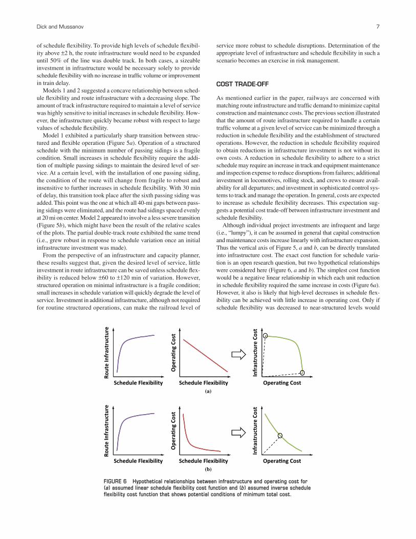
Although individual project investments are infrequent and large (i.e., “lumpy”), it can be assumed in general that capital construction and maintenance costs increase linearly with infrastructure expansion. Thus the vertical axis of Figure 5, a and b, can be directly translated into infrastructure cost. The exact cost function for schedule varia-tion is an open research question, but two hypothetical relationships were considered here (Figure 6, a and b). The simplest cost function would be a negative linear relationship in which each unit reduction in schedule flexibility required the same increase in costs (Figure 6a). However, it also is likely that high-level decreases in schedule flex-ibility can be achieved with little increase in operating cost. Only if schedule flexibility was decreased to near-structured levels would

FIGURE 6 Hypothetical relationships between infrastructure and operating cost for (a) assumed linear schedule flexibility cost function and (b) assumed inverse schedule flexibility cost function that shows potential conditions of minimum total cost.

Rout

e In

fras

truc

ture

Infr

astr

uctu

re C

ost

Ope

ratin

g Co

st

Schedule Flexibility Schedule Flexibility Operating Cost(a)

(b)

Rout

e In

fras

truc

ture

Infr

astr

uctu

re C

ost

Ope

ratin

g Co

st

Schedule Flexibility Schedule Flexibility Operating Cost

8 Transportation Research Record 2546

operating costs quickly escalate (Figure 6b). Either assumption can be used to transform an equal level-of-service contour from Figure 5 into a hypothetical curve that illustrates a trade-off between capital cost (infrastructure) and operating cost (schedule flexibility). The point on this curve closest to the origin represents the optimal lowest-cost operating condition for that level of service.

For the assumption of linear schedule flexibility cost, the final curve is a concave function (Figure 6a), which suggests that one end of the curve (i.e., either a purely structured operation on minimum infrastructure or a purely flexible operation on expanded infrastruc-ture) offers the lowest total cost. However, for the assumption of an inverse schedule flexibility cost function, the final curve may be slightly convex (Figure 6b), which suggests that some compromise between infrastructure investment and schedule flexibility may mini-mize total costs. To determine which of these conditions is typical of North American rail lines requires future research into the exact form of the schedule flexibility cost function.

cOncluSiOnS and Future WOrk

For a given traffic volume and track infrastructure, train delay increases as schedule flexibility increases. However, for the corridors considered in this research, a track infrastructure condition became insensitive to further increases in schedule flexibility beyond ±120 min. Efforts to reduce delay and improve levels of service through a reduction in schedule flexibility showed little return until operations moved to highly structured conditions with little flexibility.

For a given traffic volume, a desired level of service can be achieved through different combinations of schedule variation and infrastruc-ture according to a concave relationship. Operations that minimize infrastructure investment through structured schedules with little flex-ibility are sensitive to disruptions that introduce variation in depar-ture times. Small increases in schedule flexibility require substantial investments in infrastructure to maintain the desired level of service. However, once an initial infrastructure investment is made to a certain level, the route becomes robust with respect to further increases in schedule flexibility.

Although the above conclusions are apparent for the studied single track and partial double-track routes, additional research is required to determine if consistent results are observed for other operating con-ditions. Heterogeneous traffic mixtures with passenger and priority intermodal trains may be more sensitive to schedule flexibility than homogeneous freight scenarios. Schedule flexibility may also have effects on yards and terminals not studied in this research.

Further research is required to quantify the cost trade-off between schedule variation and infrastructure investment for a given rail line capacity. Hypothetical relationships on the basis of the results of this research suggest that, under certain conditions, total railroad costs may be minimized through a compromise between schedule flexibil-ity and infrastructure investment. Other conditions may favor purely flexible or purely structured operations. Knowledge of the trade-off between schedule flexibility and infrastructure investment can help railway practitioners make optimal decisions about infrastructure expansion and train service design.

acknOWledgMentS

This research was supported by the Association of American Railroads and the National University Rail Center. The second author also was supported by the University of Illinois at Urbana–Champaign (UIUC)

Department of Civil and Environmental Engineering Research Expe-rience for Undergraduates Program. The authors thank Eric Wilson of Berkeley Simulation Software LLC for the provision of RTC and Mei-Cheng Shih of UIUC for assistance in the conduct of RTC simulations.

reFerenceS

1. Association of American Railroads. Freight Railroad Capacity and Investment. Washington, D.C., May 2015.

2. Association of American Railroads. Analysis of Class 1 Railroads. Washington, D.C., 2012.

3. American Railway Engineering and Maintenance-of-Way Association. 2014 Manual for Railway Engineering. Chapter 16. Lanham, Md., 2014.

4. Shih, M.-C., C. T. Dick, and C. P. L. Barkan. Impact of Passenger Train Capacity and Level of Service on Shared Rail Corridors with Multiple Types of Freight Trains. In Transportation Research Record: Journal of the Transportation Research Board, No. 2475, Transportation Research Board of the National Academies, Washington, D.C., 2015, pp. 63–71.

5. Dingler, M. H., Y.-C. Lai, and C. P. L Barkan. Effect of Train-Type Heterogeneity on Single-Track Heavy Haul Railway Line Capacity. Proceedings of the Institution of Mechanical Engineers, Part F: Journal of Rail and Rapid Transit, Vol. 228, No. 8, 2014, pp. 845–856.

6. Sogin, S. L., Y.-C. Lai, C. T. Dick, and C. P. L. Barkan. Comparison of Capacity of Single- and Double-Track Rail Lines. In Transportation Research Record: Journal of the Transportation Research Board, No. 2374, Transportation Research Board of the National Academies, Washington, D.C., 2013, pp. 111–118.

7. Krueger, H. Parametric Modeling in Rail Capacity Planning. Proc., Winter Simulation Conference, Phoenix, Ariz., 1999, pp. 1194–1200.

8. Higgins, A., E. Kozan, and L. Ferreira. Heuristic Techniques for Single Line Train Scheduling. Journal of Heuristics, Vol. 3, No. 1, 1997, pp. 43–62.

9. Shih, M.-C., Y.-C. Lai, C. T. Dick, and M.-H. Wu. Optimization of Sid-ing Location for Single-Track Lines. In Transportation Research Record: Journal of the Transportation Research Board, No. 2448, Transportation Research Board of the National Academies, Washington, D.C., 2014, pp. 71–79.

10. Pouryousef, H., P. Lautala, and T. White. Railroad Capacity Tools and Methodologies in the U.S. and Europe. Journal of Modern Transportation, Vol. 23, No. 1, 2015, pp. 30–42.

11. Furtado, F. M. B. A. U.S. and European Freight Railways: The Differ-ences that Matter. Journal of the Transportation Research Forum, Vol. 52, No. 2, 2013, pp. 65–84.

12. Lindfeldt, O. Railway Operation Analysis: Evaluation of Quality, Infrastructure, and Timetable on Single and Double-Track Lines with Analytical Models and Simulation. PhD dissertation. KTH Royal Institute of Technology, Stockholm, Sweden, 2010.

13. Huntley, C. L., D. E. Brown, D. E. Sappington, and B. P. Markowicz. Freight Routing and Scheduling at CSX Transportation. Interfaces, Vol. 25, No. 3, 1995, pp. 58–71.

14. Ping, L., N. Axin, J. Limin, and W. Fuzhang. Study on Intelligent Train Dispatching. Proc., 2001 Intelligent Transportation Systems Conference, Oakland, Calif., 2001, pp. 949–953.

15. Lu, Q., M. Dessouky, and R. C. Leachman. Modeling Train Movements Through Complex Rail Networks. ACM Transactions on Modeling and Computer Simulation, Vol. 14, No. 1, 2004, pp. 48–75.

16. Shih, M.-C., C. T. Dick, S. L. Sogin, and C. P. L. Barkan. Comparison of Capacity Expansion Strategies for Single-Track Railway Lines with Sparse Sidings. In Transportation Research Record: Journal of the Trans-portation Research Board, No. 2448, Transportation Research Board of the National Academies, Washington, D.C., 2014, pp. 53–61.

17. Atanassov, I., and C. T. Dick. Influence of Siding Connection Length, Posi-tion, and Order on the Incremental Capacity of Transitioning from Single to Double Track. Presented at 94th Annual Meeting of the Transportation Research Board, Washington, D.C., 2015.

18. Sogin, S., C. T. Dick, Y.-C. Lai, and C. P. L. Barkan. Analyzing the Incre-mental Transition from Single to Double Track Railway Lines. Proc., Inter-national Association of Railway Operations Research 5th International Seminar on Railway Operations Modelling and Analysis, Copenhagen, Denmark, 2013.

The Standing Committee on Freight Rail Transportation peer-reviewed this paper.