1

Analyzing Operational Flexibilityof Electric Power Systems

Andreas Ulbig and Goran AnderssonPower Systems Laboratory, ETH Zurich, Switzerland

ulbig | andersson @ eeh.ee.ethz.ch

Abstract

Operational flexibility is an important property of electric power systems and plays a crucial role forthe transition of today’s power systems, many of them based on fossil fuels, towards power systems thatcan efficiently accommodate high shares of variable Renewable Energy Sources (RES). The availabilityof sufficient operational flexibility in a given power system is a necessary prerequisite for the effectivegrid integration of large shares of fluctuating power in-feed from variable RES, especially wind powerand Photovoltaics (PV). This paper establishes the necessary framework for quantifying and visualizingthe technically available operational flexibility of individual power system units and ensembles thereof.Necessary metrics for defining power system operational flexibility, namely the power ramp-rate, powerand energy capability of generators, loads and storage devices, are presented. The flexibility propertiesof different power system unit types, e.g. load, generation and storage units that are non-controllable,curtailable or fully controllable are qualitatively analyzed and compared to each other. Quantitative resultsand flexibility visualizations are presented for intuitive power system examples.

Index Terms

Operational Flexibility, Operational Constraints, Power System Analysis, Grid Integration of Renew-able Energy Sources (RES)

I. Introduction

This paper presents a novel approach for analyzing the available operational flexibility of a givenpower system. In the context of this paper we mean by this the combined available operationalflexibility that an ensemble of diverse power system units in a geographically confined grid zonecan provide in each time-step during the operational planning, given load demand and RenewableEnergy Sources (RES) forecast information, as well as in real-time in case of a contingency. Op-erational flexibility is essential for mitigating disturbances in a power system such as outages orforecast deviations of either power in-feed, i.e. from wind turbines or solar units, or power out-feed,i.e. load demand. Metrics for assessing the technical operational flexibility of power systems, i.e.power ramp-rate (ρ), power capacity (π) and energy capacity (ε), have been proposed by Makarovet al. in [1] and their meaning further discussed by the authors in [2]. In this paper we establish thenecessary framework for quantifying and visualizing the technically available operational flexibilityof individual power system units and ensembles thereof. The functional modeling of all powersystem units is accomplished using the Power Nodes modeling framework introduced in [3], [4]. Theflexibility properties of different power system unit types, e.g. load, generation and storage unitsthat are non-controllable, curtailable or fully controllable are qualitatively analyzed and comparedto each other. Quantitative results as well as flexibility visualizations of the here proposed flexibilityassessment framework are presented for intuitive benchmark power systems.

The remainder of this paper is organized as follows: Section II discusses operational flexibility andits role in power system operation. It also introduces necessary metrics for operational flexibility.Section III explains how operational flexibility can be modeled using the Power Nodes functional

arX

iv:1

312.

7618

v2 [

mat

h.O

C]

27

Jul 2

014

2

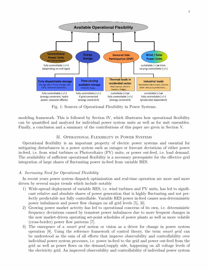
Fig. 1: Sources of Operational Flexibility in Power Systems.

modeling framework. This is followed by Section IV, which illustrates how operational flexibilitycan be quantified and analyzed for individual power system units as well as for unit ensembles.Finally, a conclusion and a summary of the contributions of this paper are given in Section V.

II. Operational Flexibility in Power Systems

Operational flexibility is an important property of electric power systems and essential formitigating disturbances in a power system such as outages or forecast deviations of either powerin-feed, i.e. from wind turbines or Photovoltaics (PV) units, or power out-feed, i.e. load demand.The availability of sufficient operational flexibility is a necessary prerequisite for the effective gridintegration of large shares of fluctuating power in-feed from variable RES.

A. Increasing Need for Operational Flexibility

In recent years power system dispatch optimization and real-time operation are more and moredriven by several major trends which include notably

1) Wide-spread deployment of variable RES, i.e. wind turbines and PV units, has led to signifi-cant relative and absolute shares of power generation that is highly fluctuating and not per-fectly predictable nor fully controllable. Variable RES power in-feed causes non-deterministicpower imbalances and power flow changes on all grid levels [5], [6].

2) Growing power market activity has led to operational concerns of its own, i.e. deterministicfrequency deviations caused by transient power imbalances due to more frequent changes inthe now market-driven operating set-point schedules of power plants as well as more volatile(cross-border) power flow patterns [7].

3) The emergence of a smart grid notion or vision as a driver for change in power systemoperation [8]. Using the reference framework of control theory, the term smart grid canbe understood as the sum of all efforts that improve observability and controllability overindividual power system processes, i.e. power in-feed to the grid and power out-feed from thegrid as well as power flows on the demand/supply side, happening on all voltage levels ofthe electricity grid. An improved observability and controllability of individual power system

3

units should also lead to an improved observability and controllability of the entire powersystem and the processes happening therein.

Altogether, these developments constitute a major paradigm shift for the management of powersystems. Operating power systems optimally in this more complex environment requires a more de-tailed assessment of available operational flexibility at every point in time for effectively mitigatingthe outlined disturbances.

Operation flexibility in power system operation and dispatch planning is of importance and hasa significant commercial value. Ancillary service markets enable system operators the cost-effectiveprocurement of needed control reserve products. In the case of frequency control schemes whichare in essence a set of differently structured flexibility services provided to system operators forachieving active power regulation on different time-scales [9], the overall remuneration for providingcontrol power and energy on ancillary service markets is usually significantly higher than for bulkenergy from spot markets [10]. The value of operational flexibility can also be shown indirectly bylooking at the inflexibility costs incurred by conventional generation units in the form of rampingcosts as well as power plant start/stop costs. In some power markets, the real or merely perceivedinflexibility of generator units to reduce their power output from planned set-points appears in theform of negative bids in the supply-side curve of the merit order [11], [12]. Negative bids may eitherreflect costs that would be incurred in case a plant’s power output is lowered, e.g. lower efficiencyas well as wear and tear, or the goal to keep a certain power plant online, i.e. must-run units thatprovide ancillary services or RES units that have in-feed priority.

B. Sources of Operational Flexibility

Different sources of power system flexibility exist as is illustrated in Fig. 1. Operational flexibilitycan be obtained on the generation-side in the form of dynamically fast responding conventionalpower plants, e.g. gas or oil-fueled turbines or rather flexible modern coal-fired power plants andon the demand-side by means of adapting the load demand curve to partially absorb fluctuatingRES power in-feed. In addition to this, RES power in-feed can also be curtailed or, in more generalterms, modulated below its given time-variant maximum output level. Furthermore, stationarystorage capacities, e.g. hydro storage, Compressed Air Energy Storage (CAES), stationary batteryor fly-wheel systems, as well as time-variant storage capacities, e.g. electric vehicle fleets, are well-suited for providing operational flexibility.

Additional flexibility can be obtained from other grid zones via the electricity grid’s tie-linesin case that the available operational flexibility in one’s own grid zone is not sufficient or moreexpensive than elsewhere. Power import and export, nowadays facilitated by more and more inte-grated transnational power markets, is used in daily power system operation to a certain degree asa slack bus for fulfilling the active power balance and mitigating power flow problems of individualgrid zones by tapping into the flexibility potential of other grid zones. For power system operation,importing needed power in certain situations and exporting undesirable power in-feed in othersituations to neighboring grid zones is for the time being probably the most convenient andcheapest measure for increasing operational flexibility. However, power import/export can onlybe performed within the limits given by the agreed line transfer capacities between the grid zones.In the European context this corresponds to the Net Transfer Capacity (NTC) values [13], whichare a rather conservative measure of available grid electricity transfer capacity.

In liberalized power systems, operational flexibility is traded in the form of energy productsvia power markets, i.e. day-ahead and intra-day spot markets, as well as control reserve products,i.e. primary/secondary/tertiary frequency control reserves, from Ancillary Services (AS) markets.

4

C. Definitions of Operational Flexibility

The term Operational Flexibility in power systems, or simply flexibility is often not properlydefined and may refer to very different things, ranging from the quick response times of certaingeneration units, e.g. gas turbines, to the degree of efficiency and robustness of a given powermarket setup. The topic has received wide attention in recent years [1], [2], [6], [14]–[16].

In the following the focus is on the basic technical capability of individual power system unitsto modulate power and energy in-feed into the grid, respectively power out-feed out of the grid.

D. Metrics for Operational Flexibility

For analysis purposes, this technical capability needs to be characterized and categorized byappropriate flexibility metrics. A valuable method for assessing the needed operational flexibilityof power systems, for example for accommodating high shares of wind power in-feed, has beenproposed by Makarov et al. in [1]. There, the following metrics have been characterized:

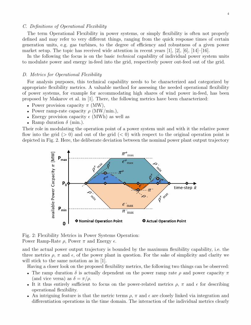
• Power provision capacity π (MW),• Power ramp-rate capacity ρ (MW/min.),• Energy provision capacity ε (MWh) as well as• Ramp duration δ (min.).

Their role in modulating the operation point of a power system unit and with it the relative powerflow into the grid (> 0) and out of the grid (< 0) with respect to the original operation point isdepicted in Fig. 2. Here, the deliberate deviation between the nominal power plant output trajectory

Fig. 2: Flexibility Metrics in Power Systems Operation:Power Ramp-Rate ρ, Power π and Energy ε.

and the actual power output trajectory is bounded by the maximum flexibility capability, i.e. thethree metrics ρ, π and ε, of the power plant in question. For the sake of simplicity and clarity wewill stick to the same notation as in [1].

Having a closer look on the proposed flexibility metrics, the following two things can be observed:

• The ramp duration δ is actually dependent on the power ramp rate ρ and power capacity π(and vice versa) as δ = π/ρ.

• It it thus entirely sufficient to focus on the power-related metrics ρ, π and ε for describingoperational flexibility.

• An intriguing feature is that the metric terms ρ, π and ε are closely linked via integration anddifferentiation operations in the time domain. The interaction of the individual metrics clearly

5

exhibit so-called double integrator dynamics: energy is the integral of power, which in turn isthe integral of power ramp-rate (Eq. 1). The three metrics constitute a flexibility trinity inpower system operation, as they cannot be thought of independently due to the inter-temporallinking.

Ramp-Rate Power Energy[MW/min.] [MW] [MWh]∫

dt∫dt

ρ � π � εddt

ddt

(1)

Using these three flexibility metrics instead of only one, for example the power ramping capability ρas in [15], allows a more accurate and complete representation of power system flexibility, includingthe relevant inter-temporal constraints over a given time interval. The power ramp-rate for absorbinga disturbance event, measured in MW/min, in a power system may be abundant at a certain timeinstant. But for a persistent disturbance, the maximum regulation power that can be providedby a generator is limited as is the maximum regulation energy that can be provided by storageunits, which are inherently energy-constrained. As the share of storage units in power systems andtheir importance for the grid integration of RES in-feed is rising, the inter-temporal links betweenproviding ramping capability and eventually reaching power/energy limits cannot be neglected whenassessing the available operational flexibility of a power system.

Having defined these flexibility metrics as well as the causal inter-linking between them (Fig. 3),allows the assessment of the available operational flexibility of an individual power system unit andfor whole power systems. Note that the operational constraints, i.e. min/max ramping, power andenergy constraints, of individual power system units have to be considered when assessing theiravailable operational flexibility.

Fig. 3: Inter-temporal linking of flexibility metrics including internal storage losses (dissipation).

III. Modeling of Operational Flexibility

The analysis and assessment of operational flexibility first of all necessitates a modeling frameworkthat allows to explicitly include information on the degree of freedom for shifting operation set-points so as to modulate the power in-feed and out-feed patterns of individual power system units.This includes information on whether or not a unit has a storage and is thus energy-constrained,whether or not a unit provides fluctuating power in-feed, and what type of controllability and

6

Fig. 4: Power Node model of an energy storage unit with power in-feed (ugen) and out-feed (uload).

observability, including predictability that a system operator has over fluctuating generation anddemand processes (i.e. full, partial or none). The combination of all these properties defines a unit’soperational flexibility.

For our modeling purposes we use the Power Nodes modeling framework, which allows thedetailed functional modeling of power system units such as

• diverse storage units, e.g. batteries, fly-wheels, pumped hydro, CAES, ...,• diverse generation units, e.g. fully dispatchable conventional generators, variably in-feeding

power units, e.g. wind turbine and PV units, and• diverse load units, e.g. conventional (non-controllable), interruptible or thermal (both partially

controllable), ...,

including their operational constraints as well as relevant information of their underlying powersupply and demand processes. Operational constraints such as min/max ramp rates, min/maxpower set-points and energy storage operation ranges, information of the underlying power systemprocesses (i.e. fully controllable, curtailable/sheddable or non-controllable) as well as informationon observability and predictability of underlying power system processes (i.e. state measures and/orstate-estimation and prediction of fully or only partially observable/predictable system and controlinput states) can also be included. The workings of the Power Node notation are illustrated bythe model representation of an energy storage unit (Fig. 4). The provided and demanded energiesare lumped into an external process termed ξ, with ξ < 0 denoting energy use and ξ > 0 energysupply. The term ugen describes a conversion corresponding to a power generation with an efficiencyηgen, while uload describes a conversion corresponding to consumption with an efficiency ηload. Theintroduction of generic energy storages in the Power Nodes framework adds a modeling layer toclassical power system modeling. Its energy storage level, the State-of-Charge (SOC), is normalizedto 0 ≤ x ≤ 1 with an energy storage capacity C ≥ 0. The illustrated storage unit serves as abuffer between the external process ξ and the two grid-related power exchanges ugen ≥ 0 anduload ≥ 0. Internal energy losses associated with energy storage, e.g. physical, state-dependentdissipation losses, are modeled by the power dissipation term v(x) ≥ 0, while enforced energylosses, e.g. curtailment/shedding of a power supply or demand process, are denoted by the wastepower term w, where w > 0 denotes a loss of provided energy and w < 0 an unserved load demand.

7

The dynamics of a power node i ∈ N = {1, . . . , N}, which can be nonlinear in the general case,are:

Ci xi = ηload,i uload,i − η−1gen,i ugen,i + ξi − wi − vi,

s.t. (a) 0 ≤ xi ≤ 1 ,

(b) 0 ≤ umingen,i ≤ ugen,i ≤ umax

gen,i ,

(c) 0 ≤ uminload,i ≤ uload,i ≤ umax

load,i ,

(d) umingen,i ≤ ugen,i ≤ umax

gen,i ,

(e) uminload,i ≤ uload,i ≤ umax

load,i ,

(f) 0 ≤ ξi · wi ,

(g) 0 ≤ |ξi| − |wi| ,

(h) 0 ≤ vi . (2)

Depending on the specific process represented by a Power Node, each term in the Power Nodeequation may be controllable or not, observable or not, and driven by an external process or not.Internal dependencies, such as a state-dependent loss term vi(xi), are possible. Charge and dischargeefficiencies may be non-constant and possibly also state-dependent: ηload,i(xi), ηgen,i(xi). Non-linearconversion efficiencies can be arbitrarily well approximated by a set of Piece-wise Affine (PWA)linear equations. The constraints (a)–(h) denote a generic set of requirements on the variables.They are to express that (a) the state of charge is normalized, (b)–(e) the grid power in-feedsand out-feeds as well as their time derivatives (ramp-rates) are non-negative and constrained, (f)the supply or demand and the curtailment need to have the same sign, (g) the supply/demandcurtailment cannot exceed the supply/demand itself, and (h) the storage losses are non-negative.The explicit mathematical form of a power node equation depends on the particular modelingcase. The notation provides technology-independent categories that can be linked to evaluationfunctions for energy and power balances. Power nodes can also represent energy processes that areindependent of storage, such as fluctuating RES generation.

More details on the Power Node modeling framework, modeling examples and reasoning can beobtained from [3], [4].

IV. Analyzing Operational Flexibility

The functional representation of complex power system interactions using the Power Nodesnotation allows a straight-forward analysis of the three power-related operational flexibility metrics,i.e. power ramp-rate ρ, power π and energy capability ε.

A. Quantification of Operational Flexibility

Taking as an example the operational flexibility of a generation unit i that has an inherentstorage function and the possibility for curtailment, e.g. a hydro storage lake, given by the PowerNode model

Ci xi = −η−1gen,i ugen,i + ξi − wi − vi , (3)

for providing power regulation is accomplished by calculating the set of all feasible power regulationpoints {π±

i (k)}, where up/down power regulation is denoted by ’+/−’ respectively, based onequation {

π±i (k)

}={ufeasiblegen,i (k)

}− u0gen,i(k) (4)

={ηgen · (ξ − w − vx − Cx)

}k,i− u0gen,i(k)

s.t. 0 ≤ umingen,i(k) ≤ {ufeasiblegen (k)} ≤ umax

gen,i(k) .

8

Fig. 5: Flexibility cube of maximum available operational flexibility of a generic power system unit.

Fig. 6: Time-evolution of maximum available operational flexibility (k = 24 h, 36 h, 48 h, 60 h).

Here, u0gen,i(k) denotes the nominal (actual) set-point of the generation unit and the term ufeasiblegen,i (k)represents an arbitrary set-point from the set of all feasible operating points {·} to which the unitcan be steered to provide operational flexibility. Both terms can be chosen to be time-variant.They are given here for time-step k. The set of all feasible operation points thus depends upon theinternal status of the generation unit, as defined by the terms ξi(k), wi(k), vi(xi(k)) and Cixi(k),and bounded by the unit’s power rating constraints (Eq. 2 (b–d)).

9

The maximum available flexibility for up/down power regulation is given as

π+max,i(k)=min

[ηgen

(ξmax − wmin − vx − Cx

), umax

gen

]k,i

−u0gen,i(k) ,

π−min,i(k) =max

[ηgen

(ξmin − wmax − vx − Cx

), umin

gen

]k,i

−u0gen,i(k) , (5)

in which wmini (k) and wmax

i (k) define the min./max. allowable curtailment for generation unit i attime-step k. In case the primary fuel supply is controllable, the terms ξmin

i (k) and ξmaxi (k) define the

minimum/maximum allowable primary power provision. Please note that the sign of the storagepower term Cx is negative when providing positive power, i.e. discharging (Cx < 0), and positivewhen providing negative power, i.e. charging (Cx > 0). In the time-discrete case the term Cxbecomes Cδx = C(x(k)− x(k − 1) ).

This flexibility assessment for metric π (Eq. 4–5) can be extended to other two metrics, ρ and ε,via time-differentiation and integration, respectively. The flexibility assessment for all other powersystem unit types can be accomplished in a similar fashion. Please note that the maximum availableflexibility calculated in this way is without any consideration of how long a certain power systemunit would need to reach a new operation point that allows this provision of flexibility.

B. Visualization of Operational Flexibility

The three thus calculated flexibility metrics span a so-called flexibility volume, which can berepresented in its simplified form as a flexibility cube for a generic power system unit i, with theterms π+, π−, ρ+, ρ−, ε+, ε− as its vertices or extreme points. A qualitative illustration of this isshown in Fig. 5, where the flexibility volume is cut into eight separate sectors.

The evolution over time of the (maximum) available operational flexibility from a generic storageunit with both load and generation terms, uload(k) and ugen(k), is illustrated in Fig. 6. The plotsshow that the available operational flexibility is highly time-variant due to the actual storage usageover time.

However, when taking into account the internal double-integrator dynamics, the flexibility volumebecomes a significantly more complex polytope object. An illustration of this more realistic polytopeflexibility volume is given by Fig. 7. Here, the information of how long it takes to reach a certainnew operation point providing a required set {ρ, π, ε} of operational flexibility is explicitly given.The set of reachable operation points providing additional flexibility (green) becomes larger whenthe available time span is longer. The flexibility set converges towards the set of maximal flexibility(red) as defined by the underlying technical constraints of a given power system unit. Calculatingthe available set of operational flexibility that is achievable after a given number of time-stepsk is equivalent to a classical reach set calculation. This later approach, although more exact,is significantly more computationally expensive than the simpler analytic approach sketched outpreviously by Eq. (4–5).

For the reach-set calculations, the reachability functions of the MPT Toolbox [17] have beenused in Matlab. There a so-called polytope method is employed that involves besides other thingsthe calculation of the Controllability Gramian WC . (See [18, p. 19 ff.] for a general discussion ofreachability analysis.) The advantage of the MPT Toolbox is that it explicitly allows the usage ofbox constraints for inputs and states of dynamical systems. In power systems, a typical example ofa box constraint are the limitations on min/max power ramp-rate, e.g. umin

gen. ≤ ugen. (k) ≤ umaxgen. , and

min/max power output, e.g. umingen. ≤ ugen. (k) ≤ umax

gen. . Other approaches for calculating gramiansand the corresponding reach-sets include Linear Matrix Inequalities (LMI) methods, as explainedin [19], as well as so-called ellipsoidal methods, which have been implemented for example in theEllipsoidal Toolbox [20].

10

Fig. 7: Evolution of available operational flexibility from a storage unit at its planned operationpoint (k = 0).Green: Time-evolution of available flexibility after k = 1h, 2h, 3h, 5h, 10h, 15h (calculated viareach sets).Red: Maximum available operational flexibility at k →∞ (calculated using Eq. (4–5)).

Please note that the theoretical maximum reachability volume calculated by the analytic ap-proach may in fact never be fully reached by the power system unit, when using the reach setapproach (Fig. 7). This gap is due mainly to the non-infinite discrete sampling time in combinationwith somewhat pathological operation points at some of the flexiblity cube’s vertices, e.g. fullydischarging a storage unit (π−) while at the same time keeping it at its maximum energy storagelevel (ε+).

C. Aggregation of Operational Flexibility

An important question in power system analysis is how a group or pool of power system unitsact together in achieving a given objective, i.e. delivering a scheduled power trajectory or providing

11

ancillary services by tracking a control signal. Pooling together different power system units toprovide a service that they cannot provide individually is an active research field. A prime example isto combine a dynamically slow power plant with a dynamically fast, but energy-constrained storageunit to provide fast frequency regulation that neither of the units could provide individually [21] dueto the lack of one flexibility metric, i.e. the missing fast ramp-rate capability ρ of the power plant, oranother, i.e. the small energy capability ε of the storage unit. Obtaining the aggregated operationalflexibility that a pool of different power system units provides, is equivalent to aggregating theflexibility volumes of the individual units. Since these are given by more or less complex polytopesets, depending on the chosen calculation approach presented in the previous section, a well-knownpolytope operation, the Minkowski Summation, can be employed for calculating the aggregatedflexibility of the pool. In the following, we illustrate the aggregation of a slow-ramping power planttogether with a fast-ramping but energy-constrained storage unit in Fig. 8. We assume that withinthe grid zone of a unit pool, grid constraints are minor and not of practical relevance for thequantification of aggregated flexibility. Although this is a simplifying assumption, it is often used,e.g. in power markets operation.

The aggregation of two or more power system units leads to the addition of individual flexibilitymetrics

{ρ, π, ε}agg = {ρ, π, ε}slow + {ρ, π, ε}fast . (6)

The aggregation of the operational flexibility of both units, given individually by their respectivepolytope objects, is accomplished via Minkowski Summation

ρ+agg =∑i

ρ+i , ρ−agg =∑i

ρ−i ,

π+agg =

∑i

π+i , π−

agg =∑i

π−i , (7)

ε+agg =∑i

ε+i , ε−agg =∑i

ε−i .

The slow-ramping unit, e.g. a thermal power plant, with {ρ, π, ε}slow, is assumed to have anunlimited fuel supply, which implies that no energy constraints exist and that the energy provisioncapability is infinite (εslow = ∞). Also, the potential power output π is large. Dynamically slowmeans in this context that the power ramp-rate ρ is small. The fast-ramping storage unit, e.g. afly-wheel or battery system, with {ρ, π, ε}fast, has a limited run-time bounded by energy constraintsof the storage unit and thus only a limited energy storage capability exists (0 < εfast �∞).

As is often the case for storage units, ramp-rate ρ is large whereas power capability π is com-paratively small. Depending on storage technology, time-dependent storage losses, v(x), can besignificant. This is notably the case of fly-wheel energy storage systems, where storage losses dueto bearing friction become large when going beyond a storage cycle duration of a few minutes.

D. Available versus Needed Operational Flexibility

At last we compare the needed operational flexibility for mitigating a disturbance event with theavailable flexibility that a given power system can offer. The needed flexibility could, for example,be derived from the assumed worst-case succession of the combined wind and PV in-feed forecasterrors over a given time interval (see [1] as an illustration of needed flexibility for balancing windforecast errors in the CAISO grid).

Effectively balancing this requires the ability to follow steep power ramps as well as to providelarge amounts of regulating power and energy over time. In order for a given power system tosuccessfully accommodate such a disturbance event, the available flexibility volume should alwaysenvelope the needed flexibility volume, as shown in Fig. 9. If this would not be the case, flexibility

12

capability is lacking along at least one axis of the flexibility metrics (e.g. π+agg. = 0). The disturbance

event could not be fully accommodated. Calculating the polytope of the still available operationalflexibility that remains while mitigating the expected disturbance boils down to another polytopeoperation, the Pontryagin Difference.

V. Conclusion

The contributions of this paper are the presented modeling and analysis techniques for thequantitative assessment and visualization of operational flexibility in electric power systems.

We envision that these techniques will become useful tools for system operators, allowing theaggregation of the available (often too) plentiful power system state information into intuitive visualcharts, i.e. 3D images of available and needed operational flexibility cubes, and straight-forwardflexibility quantification, i.e. the flexibility metrics {ρ, π, ε}, for the current system state as well asfor predicted future system states.

This would notably allow the real-time analysis of the overall flexibility properties of unit pools, inwhich different power system units are aggregated and work together to achieve a common controlobjective (e.g. frequency and power balance regulation) but also the calculation of the remainingoperational flexibility in a power system after having subtracted the needed flexibility for mitigatinga disturbance (e.g. forecast error) from the originally available operational flexibility.

References

[1] Y. Makarov, C. Loutan, J. Ma, and P. de Mello, “Operational Impacts of Wind Generation on California Power Systems,”Power Systems, IEEE Transactions on, vol. 24, no. 2, pp. 1039 –1050, May 2009.

[2] A. Ulbig and G. Andersson, “On Operational Flexibility in Power Systems,” in IEEE PES General Meeting, San Diego,USA, July 2012.

[3] K. Heussen, S. Koch, A. Ulbig, and G. Andersson, “Energy Storage in Power System Operation: The Power NodesModeling Framework,” in IEEE PES Conference on Innovative Smart Grid Technologies (ISGT) Europe, Gothenburg,2010.

[4] ——, “Unified system-level modeling of intermittent renewable energy sources and energy storage for power systemoperation,” Systems Journal, IEEE, vol. 6, no. 1, pp. 140 –151, March 2012.

[5] T. Gul and T. Stenzel, Variability of Wind Power and other Renewables – Management Options and Strategies.OECD/IEA, Paris, 2005.

[6] L. E. Jones, Ed., Renewable Energy Integration – Practical Management of Variability, Uncertainty, and Flexibility inPower Grids. Academic Press (Elsevier), 2014.

[7] T. Weissbach and E. Welfonder, “Improvement of the Performance of Scheduled Stepwise Power Programme Changeswithin the European Power System,” in 17th IFAC World Congress, The International Federation of Automatic Control(IFAC), Seoul, Korea, 2008.

[8] US Deptartment of Energy, “Smartgrid.gov,” 2014. [Online]. Available: www.smartgrid.gov/the smart grid[9] P. Kundur, “Power system stability and control,” McGraw-Hill Inc., New York, 1994.

[10] German TSOs, “German Ancillary Service Transparency Platform,” last accessed 1 October 2013. [Online]. Available:www.regelleistung.net

[11] EPEX, “EPEX European Power Exchange,” 2012.[12] M. Nicolosi, “Wind power integration and power system flexibility – An empirical analysis of extreme events in Germany

under the new negative price regime,” Energy Policy, vol. 38, no. 11, pp. 7257 – 7268, 2010.[13] ENTSO-E, “Operation Handbook,” 2011.[14] J. Ma, V. Silva, R. Belhomme, D. Kirschen, and L. Ochoa, “Evaluating and planning flexibility in sustainable power

systems,” Sustainable Energy, IEEE Transactions on, vol. 4, no. 1, pp. 200–209, 2013.[15] E. Lannoye, D. Flynn, and M. O’Malley, “Evaluation of power system flexibility,”Power Systems, IEEE Transactions on,

vol. 27, no. 2, pp. 922–931, 2012.[16] M. Huber, D. Dimkova, and T. Hamacher, “Integration of wind and solar power in europe: Assessment of flexibility

requirements,” Energy, vol. 69, pp. 236–246, 2014.[17] M. Kvasnica, P. Grieder, and M. Baotic, “Multi-Parametric Toolbox (MPT),” 2004. [Online]. Available: http:

//control.ee.ethz.ch/˜mpt/[18] P. Gagarinov and A. A. Kurzhanskiy, “Ellipsoidal Toolbox Manual (Release 2.0 beta 1),” Tech. Rep., 19 November 2013.[19] S. Boyd, L. El Ghaoui, E. Feron, and V. Balakrishnan, Linear matrix inequalities in system and control theory. SIAM,

1994, vol. 15.[20] A. A. Kurzhanskiy and P. Varaiya, “Ellipsoidal toolbox,” EECS Department, University of California, Berkeley, Tech.

Rep. UCB/EECS-2006-46, May 2006. [Online]. Available: http://code.google.com/p/ellipsoids[21] C. Jin, N. Lu, S. Lu, Y. Makarov, and R. Dougal, “A coordinating algorithm for dispatching regulation services between

slow and fast power regulating resources,” Smart Grid, IEEE Transactions on, vol. PP, no. 99, pp. 1–8, 2013.

13

Fig. 8: Aggregation of maximum operational flexibility of individual power system units.Flexibility of conventional unit with no energy constraint (yellow), flexibility of energy-constrainedstorage (blue) and aggregated flexibility of both units (green).

Fig. 9: Needed operational flexibility versus available operation flexibility.Needed flexibility volume for balancing a disturbance (red), available flexibility volume (green) andremaining flexibility volume after subtracting the needed flexibility volume (magenta).