on the zero-inflated count models with application to modelling

Journal of Data Science 9(2011), 639-659

On the Zero-Inflated Count Models with Application toModelling Annual Trends in Incidences of Some Occupational

Allergic Diseases in France

Joseph Ngatchou-Wandji1∗ and Christophe Paris21EHESP, Rennes and Universite Henri Poincare, Nancy, France and

2Universite Henri Poincare, Nancy, France

Abstract: This paper reviews zero-inflated count models and applies themto modelling annual trends in incidences of occupational allergic asthma,dermatitis and rhinitis in France. Based on the data collected from 2001 to2009, the study uses the incidence rate ratios (IRR) as percentage of changesin incidences and plots them as function of the years to obtain trends. Theinvestigation reveals that the trend is decreasing for asthma and rhinitis, andincreasing for dermatitis, and that there is a possible positive associationbetween the three diseases.

Key words: Incidence in occupational allergic diseases, trend, zero-inflatedcount models.

1. Introduction

One generally means by count data those issued from the count of the numberof occurrences of an event of interest. Some examples of such data are, the numberof medical visit per month for a patient, the number of vehicles produced by afirm per year, the number of failures of a machine during a period. It is wellknown that count data may exhibit over/under-dispersion and/or contain toomany zeros than expected. These properties suggest the use of ad-hoc modelssuch as the so-called zero-inflated regression models or hurdle regression models,rather than the usual Poisson regression model which assumes the equality of themean and the variance of the observations.

Zero-inflated models and hurdle models are reviewed for instance, in Gschloβland Czado (2008) and Ridout et al. (1998). The reader can also refer to Grumu(1997) and Hall (2000), and references therein. These models whose story goesback at least to Mullahy (see Mullahy, 1986), have successfully been used in

∗Corresponding author.

640 Joseph Ngatchou-Wandji and Christophe Paris

econometrics, demography, medicine, public health, epidemiology, biology and inmany other fields. One of their main interesting features is that they adjust wellto data issued from a particular mixture of two populations: one in which one hasonly zero counts and another in which the counts are the realizations of a discretedistribution. An example in public health is that of a population composed of agroup of persons at risk and of a group of persons not at risk. Zero-inflated modelswould allow the occurrences of zeros in both groups while hurdle models wouldallow occurrences of zeros only in the group of persons not at risk. These twoclasses of models therefore assume that the data are issued from a mixture of twoprocesses: one generating zero counts and the other generating positive integersdata. Lambert (1992) provides a motivation application of these models anddiscusses the case of zero-inflated Poisson (ZIP) models. Other papers dealingwith these count models are amongst others, Mullahy (1986), Hall and Berenhaut(2002), Jansakul and Hinde (2001), Gupta and Gupta (2004) and Deng and Paul(2005).

Zero-inflated and hurdle models can be summarized as follows:

P (Y = y|ω) = ωδ0(y) + (1− ω)f(y), (1.1)

where Y is the count variable, ω is the proportion of the excess of zeros, δ0(y) = 1if y = 0, and = 0, otherwise, f(y) is the density of a count distribution.

One can easily observe that for f(0) = 0 and ω 6= 0, (1.1) is a hurdle model,while for f(0) 6= 0 and ω 6= 0, it is a zero-inflated model. For ω = 0, one retrievesa classical count distribution as Poisson, binomial etc. For ω > 0, (1.1) is eithera zero-inflated model or a hurdle model. For ω < 0, (1.1) is a zero-deflated modeland is no more considered as a mixture model. In the literature, f(y) is eithera binomial, a geometric, a Poisson, a negative binomial or a generalized Poissondistributions.

Once the proportion of excess of zeros is estimated, their number can easilybe estimated. The estimation can in turn be interpreted as an estimation of thelower bound of the number of occurrences of the event of interest that were notcounted. Indeed, an excess of zero count corresponds to an occurrence which,for one reason or another, is not taken into account. Therefore, in epidemiologyfor example, the knowledge of the proportion of excess of zeros in data on theincidence of a given disease can help improving the analysis of these data.

In statistics, trend can be defined as the general direction of the curve de-scribing a relationship between two variables. This notion is very familiar in themodelization of economic and financial time series where it is known as temporalor time trend. It is however also largely studied in genetic (see, eg, Texier andSellier, 1986; Zamudio et al., 2002; Bokor et al., 2007; Mourao et al., 2008; Bakiret al., 2009), and epidemiology (see, eg, Bassetti et al., 2006; Zaghloul et al., 2008;

Zero-Inflated Models for Trends Modelling 641

Hothorn et al., 2009; McNamee et al., 2009; Bateman et al., 2010). Estimatingtrend can be very useful for the sake of prediction. For example, in epidemiology,the knowledge of the trend in the incidence of a disease can help preparing usefulmaterials for containing this disease. McNamee et al. (2009) has to do with thestudy of temporal trends in some work-related skin and respiratory diseases inthe United Kindom. In this paper, the authors donnot use zero-inflated models.Instead, they use a Poisson model with a gamma random effect to modelize a setof data containing possible extra zeros.

The aim of this paper is to present zero-inflated count models, and applythem to modelling annual trends in the incidences of some occupational allergicdiseases in France. Our study is based on the idea developed in McNamee etal. (2009), with an application to the data collected from 2001 to 2009 by theReseau National de Vigilance et de Prevention des Pathologies Professionnelles(RNV3P).

This paper is organized as follows. In Section 2, we give a survey of zero-inflated models. In Section 3, we apply these models to the study of trends inthe incidences of occupational asthma, rhinitis and dermatitis in France.

2. Survey of the Zero-Inflated Models

2.1 The Common Count Models

We first present the count models commonly encountered in literature. Themost common one is undoubtedly the Poisson regression model. The Poissondistribution with parameter µ > 0, denoted by P (µ) is defined by:

P (Y = y|µ) =e−µµy

y!, y = 0, 1, 2, · · · .

It is well known that for this distribution, the expectation equals the variance.That is, E(Y = y|µ) = V ar(Y = y|µ) = µ. In the Poisson regression the responseYi’s are independent, and each Yi ∼ P (µi), µi > 0, i = 1, 2, . . . , n, with meanexpressed in terms of some covariables xi and the unknown regression parametersvector β: E(Yi = yi|xi, β) = µi(xi, β) = µi > 0. In general, µi(xi, β) = exp(xiβ),i = 1, 2, · · · , n.

An alternative to the Poisson regression model is the negative binomial re-gression model which takes into account a possible over-dispersion of the data.The distribution of the negative binomial distribution with parameters r > 0 andµ > 0, denoted by NB(r, µ) is given by:

P (Y = y|r, µ) =Γ(y + r)

Γ(r)y!

(r

µ+ r

)r ( µ

µ+ r

)y, y = 0, 1, 2, · · · ,


where for α > 0,

Γ(α) =

∫ ∞0

xα−1e−xdx.

For this distribution, one can easily prove that E(Y = y|µ) = µ and V ar(Y =y|r, µ) = µ (1 + µ/r) = µϕ. This last equality clearly shows that ϕ is the over-dispersion factor. It is immediate that for r → ∞ one retrieves the Poissondistribution with parameter µ. It would be interesting to mention that otherparametrizations use r = a−1 for a > 0.

From simple computations, one finds that if

y0 =µr − µ− r

r(2.1)

is not a positive integer, the negative binomial distribution has a unique mode at[y0] (the integer part of y0), and that if k is an integer, this distribution has twomodes at y0 and y0 + 1.

In negative binomial regression, the responses Yi’s are independent, and eachYi ∼ BN(r, µi), µi > 0, i = 1, 2, · · · , n, with mean expressed in terms of somecovariables xi and an unknown regression parameter vector β as in Poisson re-gression: E(Yi = yi|xi, β) = µi(xi, β) = µi. Here, the over-dispersed parameterϕi = 1 + µi/r depends on i.

Another alternative to the Poisson regression model is the generalized Poissonregression model. A random variable Y is said to have a generalized Poissondistribution with parameters θ and λ > 0, and denoted by GP (θ, λ) if:

P (Y = y|θ, λ) =

θ(θ + yλ)y−11

y!exp(−θ − yλ), y = 0, 1, 2, · · · ,

0, y > m for λ < 0,

where θ > 0, max(−1,−θ/m) ≤ λ ≤ 1 and m (≥ 4) is the largest positive integerfor which θ + λm > 0 when λ < 0. It is easy to show that E(Y = y|θ, λ) =θ/(1− λ) = θϕ and V ar(Y = y|θ, λ) = E(Y = y|θ, λ)ϕ2. One can remark thatϕ2 represents an over-dispersion factor. For λ = 0 this distribution reduces tothe Poisson distribution P (θ). For λ > 0 it is over-dispersed, and for λ < 0 it isunder-dispersed. Here, in contrast to the negative binomial model the dispersionfactor is the same for all observations. Another important remark is that thegeneralized Poisson distribution GP (θ, λ) is unimodal regardless the values of θand λ.

In the generalized Poisson regression model, the responses Yi’s are inde-pendent, and each Yi ∼ GP (θi, λ), i = 1, 2, · · · , n, with E(Yi = yi|xi, β, λ) =µi(xi, β) = µi > 0, for covariables xi and parameter β. One can also observe that


the equality µi = θi/(1− λ) = θiϕ leads to the following new parametrization ofthe distribution:

P (Yi = yi|xi, β, λ) = µi[µi + (ϕ− 1)yi]yi−1ϕ

−yi

yi!× exp

[−µi + (ϕ− 1)yi

ϕ

].

2.2 Inference in Parametric Zero-Inflated Models

Rewriting (1.1) with f(y) = f(y|φ) depending on an unknown parameter φ,one has:

P (Y = y|ω, φ) =

{ω + (1− ω)f(0|φ), y = 0,(1− ω)f(y|φ), y > 0.

From simple computations, one finds that the mean and the variance of thisdistribution are given by:{

E(Y |ω, φ) = (1− ω)Ef (Y |φ),

V ar(Y |ω, φ) = ω(1− ω) [Ef (Y |φ)]2 + (1− ω)V arf (Y |φ).(2.2)

Denote µL the mean of a distribution L. It results from (2.2) that for thezero-inflated Poisson ZIP (µP ) model, the mean equals (1 − ω)µP and the vari-ance equals the mean times ωµP + 1. For the zero-inflated generalized PoissonZIGP (θ, λ) model, the expectation is (1− ω)µGP while the variance equals thisnumber times µGPω+1/(1− λ)2. Finally, for the zero-inflated negative binomialZINB(r, µ) model, the mean is (1 − ω)µNB and the variance is this quantitytimes ωµBN + 1 + µNB/r. From these results, one can see that the dispersioncan result either from ω, r or λ.

Zero-inflated regression models are generally built as follows. Let Y1, · · · , Ynbe independent random variables following one of the above distributions withexpectation µL,i and proportion of excess of zeros ωi depending on individuals.For ω = (ω1, · · · , ωn), ωi > 0, i = 1, · · · , n and µ = (µL,1, · · · , µL,n), µL,i > 0,one can take {

ωi = G(z′iα),µL,i = exp(x′iβ),

(2.3)

where zi and xi are the covariables and α and β the corresponding parametervectors, and the link function G(x) being either the logistic function or the cu-mulative distribution function of a standard normal random variable:

G(x) =

exp(x)

1 + exp(x),

1√2π

∫ x

−∞exp

(−u

2

2

)du, x ∈ R.


In many situations, ωi and µL,i are assumed to be linked by some relation whichcan considerably reduce the number of parameters in the model. The most com-mon example is that where for all i = 1, · · · , n,

log

(ωi

1− ωi

)= −γ log(µL,i) ⇐⇒ ωi =

µ−γL,i

1 + µ−γL,i,

for some real parameter number γ. For positive values of γ, the zero state becomesless likely and for negative values, excess zeros become more likely.

The form of the likelihood of (1.1) at Y = (y1, · · · , yn), for ω = (ω1, · · · , ωn),and φ = (φ1, · · · , φn) is given by:

L(Y |ω, φ) =∏i:yi=0

[ωi + (1− ωi)f(0|φi)]×∏i:yi>0

[(1− ωi)f(yi|φi)] . (2.4)

When the ωi’s are expressed in terms of the covariates zi’s and parameter α, andwhen the φi = µL,i’s are expressed in terms of the covariates xi’s and parameterβ, one obtains another parametrization of the likelihood on the basis of whichinference can be done.

Parameter estimation in these models are generally done by the maximumlikelihood method. That is, by maximizing (2.4) or its logarithm after plugging-in (2.3). For doing this, one usually needs optimization methods such as Gauss-Newton, Newton-Raphson or other numerical methods. A relevant paper is Lam-bert (1992) where this estimation is considered in the case of ZIP model with thestudy of its standard errors and confidence intervals. However, parameter estima-tion by maximum likelihood method has been discussed in many papers before.In Fahrmeir and Kaufmann (1985) is studied the consistency and the asymptoticnormality of the maximum likelihood estimator of a generalized linear model. InLawless (1987) is estimated the parameters of a negative binomial model by alikelihood method and by the approach of Breslow (1984). A more recent paperin this field is Famoye and Singh (2006) where is investigated likelihood estima-tors in zero-inflated generalized Poisson regression models. Many other papersdealing with maximum likelihood estimation in these models can be found in thereferences given in the above cited papers.

As far as testing statistical hypotheses is concerned, the tests used in zero-inflated models are score-type tests. The main hypothesis tested are either theinflation of zeros, either the over-dispersion or jointly inflation of zeros and over-dispersion. Such tests are used for instance, in Mullahy (1986) for testing ageneral class of count models, and in Lawless (1987) for testing a Poisson modelagainst a negative binomial model. Most of the existing papers are, however,concerned with testing the excess of zeros. Such papers are amongst others, van


den Broek (1995) who studies a score test for testing inflation in a Poisson dis-tribution, Deng and Paul (2000) who presents a score test of goodness-of-fit fordiscrete generalized linear models against zero-inflated models, Hall and Beren-haut (2002) where is proposed a score test for heterogeneity and over-dispersionin zero-inflated and binomial regression models, Famoye and Singh (2006) whereis applied a score test for the excess of zeros in zero-inflated regression models,

Gupta and Gupta (2004) whose score test is applied to testing zero-inflatedgeneralized Poisson regression models, Deng and Paul (2000) where a score testis used for testing the inflation of zeros, the over-dispersion and jointly inflationof zeros and over-dispersion in zero-inflated generalized linear regression models.

2.3 Some Existing Applications

Zero-inflated models have been applied to many genuine data sets from var-ious sources. In Mullahy (1986) these models are applied to modelling surveymicro data on beverage consumption. In Lawless (1987) such a model is ad-justed to a set of data from ship damage incidents (see McCullagh and Nelder,1983). In Lambert (1992) zero-inflation models are applied to modelling defectsin manufacturing, while in van den Broek (1995) they are applied on data fromHIV-infected men (see Hoepelman et al.,1992). Using an hurdle model, Boharaand Krieg (1996) examines the migration frequency in the United States of Amer-ica. In Bohning et al. (1997) zero-inflated count models are used for modelingfour sets of data from dental epidemiology, traffic accidents, crime sociology andgraphic epidemiology respectively. In Deng and Paul (2000) they are adjustedto data concerning patients who experienced frequent premature ventricular con-tractions. In Famoye and Singh (2006) a such model is adjusted to a set ofdomestic violence data with many zeros. Ridout et al. (1998) illustrate theirwork with an example from horticultural research, and review a broad amount ofpapers treating biological examples of data sets modelled by zero-inflation countmodels. Another relevant paper is Gschloβl and Czado (2008) where these mod-els are applied to modelling invasive meningococcal disease in Germany. As onecan see, there is no doubt that the scope of application of these models is large.In the next section we give more applications.

3. Modelling Trends in Occupational Allergic Diseases in France

3.1 Trends in Genetics and Epidemiology Data

Trends have been studied in many fields of genetic including cattle and threes.On this subject some relevant works are, Texier and Sellier (1986) who estimategenetic trends for growth and carcass traits in two French pig breeds, Zamudio et


al. (2002) where is studied trends in wood density and radial growth with cambialage in a radiata pine progeny test, Bokor et al. (2007) where is investigatedtrends in the Hungarian racehorse populations, Mourao et al. (2008) in whichis estimated trend of meat quality traits in a male boiler line, and Bakir et al.(2009) where trends in days yield in Holstein Friesian cattle are estimated. Thestatistical tool used in these papers for the study of trends is the classical linearmodel or its extension to random effects or fixed effects models. The reason isthat the response variables and the covariates are of real nature.

Trends in general, and temporal trends in particular, have also been investi-gated in epidemiology. For instance, Hothorn et al. (2009) present some trendtests for evaluating exposure-response relationships in epidemiological exposurestudies. Using a chi-square test, Bassetti et al. (2006) study epidemiologicaltrends in nosocomial candidemia in intensive care. Zaghloul et al. (2008) studytemporal trends in patient with bladder cancer who underwent definitive surgeryalong an extended time of 17 years. The tools used for this study are ANOVA,Student and chi-square tests.

The study in McNamee et al. (2009) is of a great interest to us as it is verysimilar to what we wish to do. In this paper, the authors measure temporaltrends in the incidence of some work-related diseases in the United Kingdomfrom 1996 to 2005 on the basis of count data with possible extra zeros counts,collected by three groups of reporters spread all over the country. The authorsuse a Poisson regression model with a gamma random effects, which is equivalentto using a negative binomial regression. The dependent variable is the numberof case per reporter per month. The main covariates are months or seasons, theyears as categorial variables and as numerical variables. The authors consideredthe effects of the calendar years in the regression as incidence rate ratio (IRR).They next interpret these IRR as percentage of changes in incidence, and plotthem as functions of the calendar years to display annual trends. They modelizeseparately trends in probability of non-response. However, we think that it couldbe very interesting to treat both modelizations with one single model, by usingzero-inflated models.

3.2 The Data and the Methods

As already mentioned earlier, one of our main objectives is to model annualtrends in incidences of some occupational dermatitis and respiratory diseases inFrance from 2001 to 2009. Our work is based on data collected by the RNV3Pfrom the 32 French centres of occupational diseases, named Centre de Consulta-tion de Pathologies Professionnelles (CCPP). The diseases involved are allergicasthma, dermatitis and rhinitis.

Organization and goals of the RNV3P were described in Bonneterre et al.


(2008). Briefly, Occupational disease Departments of French University Hospi-tals reported since 2001 all cases of diseases thought to be in relation with workexposures. Each occupational health report is a structured expert clinical re-port whose principal coded items are: principal disease and co-morbid diseases(ICD-10), principal nuisance and four other possible nuisances (INRS-CNAM),professional position (ISCO-88, edited by ILO) and sector of professional activity(NAF, edited by INSEE). Each association plausibility between the principal nui-sance and nuisances was rated by an expert. The present work included all casesof asthma (J45 to J45.9 ICD-10 codes), allergic rhinitis (J30.0 to J31.0 ICD-10codes) and contact dermatitis (L23.0 to L23.9 ICD-10 codes) reported between2001 and 2009 with at least probable or certain association with one occupationalexposure.

For the study of the annual trends in the incidences of these diseases, wefollow the approach developed in McNamee et al. (2009). But rather than usinga Poisson regression models with random effects, we use ZINB regression modelsdescribed in the preceding paragraph. The dependent variable is the numberof cases per centre per month. The covariates are the months labeled Jan, FebMar, Apr, May, Jun, Jul, Aug, Sep, Oct, Nov, Dec, the years considered ascategorial variables labeled Year1, Year2, · · · , Year9, and the 32 centres labeledC01, C02, · · · , C31, C32. The reference month is August, the reference year is2004 and the reference centre is C18. We checked that these arbitrary choicesdonnot have any incidence on the trends of our data.

3.3 Numerical Results

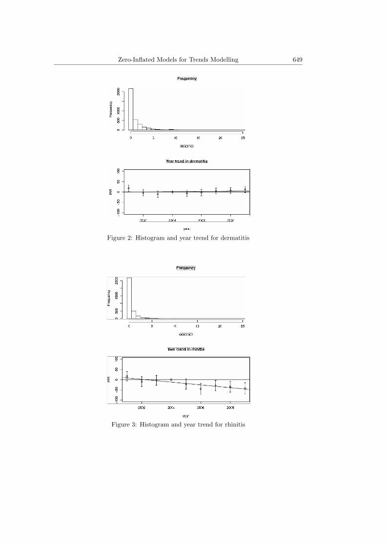
Each set of data contains n = 3456 observations that can be assumed to beindependent. Examining these data, it is seen that they comprise a large numberzeros : 2162 for asthma, 2156 for dermatitis and 2698 for rhinitis. See also thehistograms of Figures 1-3. Given this amount of zeros, it is natural to questionthe possibility of a proportion of extra zeros amongst them. Next, one finds thatfor asthma, the mean is 0.835, the variance is 2.55 and the maximal value is 22.For dermatitis, the mean is 0.977, the variance is 3.735 and the maximal value is21. Finally, for rhinitis, the mean is 0.349, the variance is 0.730 and the maximalvalue is 12. One can see that data are overdispersed as the variances are largerthan the means.

These features of our data suggest the use of zero-inflated models for theirmodelizations. Although we presented three classes of these count models, weonly used ZIP and ZINB regression models for doing this. The main reason isthat only these models are available on the software SAS that we use. But wewould like to mention also that we used R software for the study of trend testsand plotting graphics.


The zero-inflated link function, or the function G(x) we used was the logisticfunction. The covariates in this part of the model were the months and thecentres, while in the main part, in addition to these were the years as covariates.We made this choice because including the years in the zero-inflated part gives anon-linear function of the years and their effects considered as IRR’s are difficultto compute. In this situation, studying the trends in the data in the spirit ofMcNamee (2009) as we want to do is not easy. Although the relation

ωi =µ−γL,i

1 + µ−γL,i

provides more parsimonious models, it also leads to a non-linear function of theyears and can induce the difficulty mentioned earlier. Moreover, the option ofusing this relation is not available on the SAS software. For these reasons, we donot use it.

Frequency

incidence

Fre

quency

0 5 10 15 20 25

0500

1500

2002 2004 2006 2008

−100

−50

050

100

Year trend in asthma

year

IRR

Figure 1: Histogram and year trend for asthma


Figure 2: Histogram and year trend for dermatitis

Figure 3: Histogram and year trend for rhinitis


We first adjusted a ZINB regression model to each of the three sets of data.For asthma and dermatitis, the estimated dispersion parameter was too large,meaning that the overdispersion observed in the data likely comes from excess ofzeros rather than the heterogeneity among observations. Since in addition the p-value of the associated Student test was significant, we decided to modelize thesesets of data by ZIP regression models, and the rhinitis data by a ZINB regressionmodel. For each data, the likelihood, the AIC (Akaike Information Criterion)and the BIC (Bayesian Information Criterion) of the corresponding model (theone with months, years and centres in the main part and months and centresin the zero-inflated part) were both larger than those of many other competingzero-inflated regression models. Some of the latter models did not include eitherthe zero-inflated part and the centres, or the zero-inflated part and the monthsand centres, or the zero-inflated part and the years and centres, or some naivemodels such as Poisson and Negative Binomial (without any covariate).

As a checking procedure for the suitability of the models adjusted to each data,we plotted the residual series and their histograms. These series are obtained asthe difference between the observations and the predicted values from the zero-inflated modelizations. Figure 4 shows that for the three diseases, more than85 % of the residuals are within [−1, 1]. This indicates that the zero-inflatedregressions models used are good predictable models for the three sets of data.

Figure 4: Residuals plots


For the estimation of the parameters of our models, we used Newton-Raphsonalgorithm. This algorithm converged for each set of data, yielding reasonablestandard deviations of the estimators of the parameters. Table 1 presents theestimates of the parameters of the zero-inflated models for the three diseases.To save space, we do not present the associated standard deviations. It can beseen on this table that, for the three diseases, the magnitudes of the estimatesassociated with C06 and C10 are significantly different to those of the other suchcovariates. A same remark can be done for the estimates associated with Inf.C04,Inf.C05, Inf.C07, Inf.C09–Inf.C11, Inf.C22 and Inf.C25. We could not find anyexplanation to this phenomenon.

The lower plots in Figures 1-3 are those of trends. On these plots, the IRR,obtained as the coefficients of the years in the principal part of the zero-inflatedmodel, on the y-axis is multiplied by 100. It can be seen from the figures that thetrend in asthma and rhinitis is decreasing with calendar time, while it is nearlyconstant but slightly increasing in dermatitis. Kendall τ and the associated testused as trend detection provided more evidences to support these conclusions.Indeed, for asthma and rhinitis respectively, we obtained τ = −0.7222222 and−0.6666667 showing a negative association between the IRR’s and the years,a result confirmed by the p-values 0.005886 and 0.01267. For dermatitis, τ =0.3333333 showing a weak positive association between the IRR’s and the years,while the p-value = 0.2595 leads to rejecting the hypothesis of association betweenthe IRR’s and the years. That is, for dermatitis, the IRR’s are constant over theyears.

We also computed the estimated proportions of excess of zeros. To save space,we only present the results for rhinitis. The model used was a ZINB regressionmodel including months, years and centres in the main part, and months andcentres in the zero-inflated part. The results are gathered in the Table 1 fromwhich it can be seen that some of these proportions are too small. In other word,the probability to have an extra zero count in some centres at some months ofthe year is almost nil for rhinitis. But for many other centres as C25, C26, C27,C30 the probability of having an extra zero in January, February and March isvery significative.

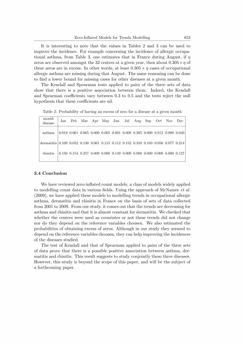
We studied the case where the proportions of zeros were functions of themonths only. That is, we considered models for which the zero-inflated part donot include centres. The results depicted in Table 2 show that the probability ofhaving an excess of zeros in France for asthma is small for all months and is farbelow 0.305 which is the probability of having an excess of zero in August. Theseprobabilities are generally higher for dermatitis with 0.31 in August and 0.214 inDecember. The same observation can be made for rhinitis, with a value of 0.257in march.


Table 1: Rhinitis : probability of having an excess of zero for a center at agiven month

monthJan Feb Mar Apr May Jun Jul Aug Sep Oct Nov Dec

centre

C01 0.011 0.039 0.435 0.017 0.005 0.020 0.008 0.0210 0.013 0.054 0.009 0.002

C02 0.001 0.006 0.096 0.002 0.001 0.003 0.001 0.003 0.002 0.008 0.001 0.000

C03 0.011 0.039 0.435 0.017 0.005 0.020 0.008 0.021 0.013 0.054 0.009 0.002

C04 0.000 0.001 0.027 0.001 0.000 0.001 0.000 0.001 0.001 0.002 0.000 0.000

C05 0.559 0.825 0.989 0.668 0.390 0.700 0.485 0.709 0.598 0.870 0.515 0.207

C06 0.012 0.044 0.470 0.020 0.006 0.023 0.009 0.024 0.014 0.062 0.010 0.003

C07 0.001 0.003 0.056 0.001 0.000 0.002 0.001 0.002 0.001 0.004 0.001 0.000

C08 0.007 0.024 0.320 0.010 0.003 0.012 0.005 0.013 0.008 0.034 0.006 0.001

C09 0.002 0.007 0.118 0.003 0.001 0.003 0.001 0.004 0.002 0.010 0.002 0.000

C10 0.005 0.019 0.273 0.008 0.003 0.010 0.004 0.010 0.006 0.027 0.004 0.001

C11 0.020 0.070 0.589 0.031 0.010 0.036 0.015 0.038 0.023 0.097 0.017 0.004

C12 0.012 0.044 0.466 0.019 0.006 0.022 0.009 0.023 0.014 0.061 0.010 0.002

C13 0.002 0.007 0.122 0.003 0.001 0.004 0.001 0.004 0.002 0.010 0.002 0.000

C14 0.132 0.361 0.915 0.195 0.071 0.219 0.102 0.226 0.151 0.445 0.113 0.030

C15 0.009 0.032 0.388 0.014 0.004 0.016 0.007 0.017 0.010 0.045 0.007 0.002

C16 0.000 0.001 0.025 0.001 0.000 0.001 0.000 0.001 0.000 0.002 0.000 0.000

C17 0.093 0.276 0.878 0.140 0.049 0.159 0.071 0.165 0.107 0.351 0.079 0.021

C18 0.003 0.013 0.197 0.005 0.002 0.006 0.003 0.007 0.004 0.018 0.003 0.001

C19 0.006 0.024 0.316 0.010 0.003 0.012 0.005 0.012 0.007 0.033 0.005 0.001

C20 0.005 0.019 0.270 0.008 0.003 0.010 0.004 0.010 0.006 0.027 0.004 0.001

C21 0.010 0.035 0.404 0.015 0.005 0.017 0.007 0.018 0.011 0.048 0.008 0.002

C22 0.010 0.037 0.422 0.016 0.005 0.020 0.007 0.019 0.012 0.052 0.008 0.002

C23 0.001 0.005 0.093 0.002 0.001 0.003 0.001 0.003 0.002 0.007 0.001 0.000

C24 0.001 0.005 0.089 0.002 0.001 0.003 0.001 0.003 0.002 0.007 0.001 0.000

C25 0.488 0.780 0.985 0.603 0.325 0.638 0.415 0.647 0.528 0.834 0.444 0.164

C26 0.698 0.896 0.994 0.786 0.538 0.810 0.632 0.816 0.730 0.924 0.659 0.322

C27 0.793 0.934 0.996 0.859 0.659 0.876 0.740 0.880 0.818 0.953 0.762 0.441

C28 0.000 0.000 0.006 0.000 0.000 0.000 0.000 0.000 0.000 0.000 0.000 0.000

C29 0.030 0.104 0.688 0.047 0.015 0.055 0.023 0.057 0.035 0.141 0.025 0.006

C30 0.757 0.920 0.995 0.831 0.610 0.851 0.698 0.856 0.784 0.942 0.722 0.398

C31 0.011 0.039 0.435 0.017 0.005 0.020 0.008 0.021 0.013 0.054 0.009 0.002

C32 0.001 0.003 0.056 0.001 0.000 0.002 0.001 0.002 0.001 0.004 0.001 0.000


It is interesting to note that the values in Tables 2 and 3 can be used toimprove the incidence. For example concerning the incidence of allergic occupa-tional asthma, from Table 3, one estimates that in France during August, if ηzeros are observed amongst the 32 centres at a given year, then about 0.305×η ofthese zeros are in excess. In other words, at least 0.305× η cases of occupationalallergic asthma are missing during that August. The same reasoning can be doneto find a lower bound for missing cases for other diseases at a given month.

The Kendall and Spearman tests applied to pairs of the three sets of datashow that there is a positive association between them. Indeed, the Kendalland Spearman coefficients vary between 0.3 to 0.5 and the tests reject the nullhypothesis that these coefficients are nil.

Table 2: Probability of having an excess of zero for a disease at a given month

monthJan Feb Mar Apr May Jun Jul Aug Sep Oct Nov Dec

disease

asthma 0.018 0.061 0.065 0.000 0.065 0.001 0.000 0.305 0.000 0.012 0.000 0.040

dermatitis 0.109 0.052 0.130 0.061 0.115 0.112 0.152 0.310 0.103 0.056 0.077 0.214

rhinitis 0.150 0.154 0.257 0.000 0.000 0.149 0.000 0.000 0.000 0.000 0.000 0.127

3.4 Conclusion

We have reviewed zero-inflated count models, a class of models widely appliedto modelling count data in various fields. Using the approach of McNamee et al.(2009), we have applied these models to modelling trends in occupational allergicasthma, dermatitis and rhinitis in France on the basis of sets of data collectedfrom 2001 to 2009. From our study, it comes out that the trends are decreasing forasthma and rhinitis and that it is almost constant for dermatitis. We checked thatwhether the centres were used as covariates or not these trends did not changenor do they depend on the reference variables choosen. We also estimated theprobabilities of obtaining excess of zeros. Although in our study they seemed todepend on the reference variables choosen, they can help improving the incidencesof the diseases studied.

The test of Kendall and that of Spearman applied to pairs of the three setsof data prove that there is a possible positive association between asthma, der-matitis and rhinitis. This result suggests to study conjointly these three diseases.However, this study is beyond the scope of this paper, and will be the subject ofa forthcoming paper.


Table 3: Parameter estimates in the ZINB regression model for the three dis-eases

covariate asthma dermatitis rhinitis

Intercept -0.979707 -1.258537 -2.249986

Jan 1.111791 0.985420 1.316493

Feb 0.880250 0.880640 1.047251

Mar 0.851777 0.900969 1.496072

Apr 0.904905 0.614507 0.875557

May 0.819898 0.730102 0.823388

Jun 0.842190 0.908627 1.125616

Jul 0.509305 0.593247 0.702703

Sep 0.723105 0.846425 0.877917

Oct 0.874790 0.922196 0.986637

Nov 0.733875 0.910171 0.998005

Dec 0.425925 0.716958 0.560845

Year1 0.450787 0.185765 0.165703

Year2 0.146011 -0.038708 -0.096014

Year3 -0.024963 -0.102079 -0.030964

Year5 -0.014721 -0.065698 -0.217263

Year6 -0.225170 -0.024604 -0.450744

Year7 -0.365657 0.045038 -0.290534

Year8 -0.165690 0.073254 -0.344327

Year9 -0.297790 0.125163 -0.424954


C01 -3.047696 -3.078948 -3.092717

C02 -0.420887 -2.436664 -1.615570

C03 -1.141717 -1.322860 -3.092495

C04 0.684000 0.306248 0.482758

C05 -0.103260 0.484544 0.690081

C06 -17.502936 -15.088005 -14.409579

C07 -0.823076 -0.341485 -0.049405

C08 -0.153315 1.228411 -0.765911

C09 1.153255 1.924443 1.869316

C10 1.758370 1.216026 1.518678

C11 -2.354550 -0.767754 -1.880624

C12 1.332860 0.877562 0.877740

C13 0.201393 0.809156 -0.000996

C14 -1.661194 -4.000277 0.659932

C16 -0.011018 1.280620 -0.232758

C17 -0.803846 -0.263222 -0.541609

C19 0.737670 2.450919 1.792409

C20 1.164689 0.899807 2.120085

C21 -17.502936 -15.088005 -14.409579

C22 1.138160 0.576202 0.900590

C23 0.001311 0.533790 -0.335585

C24 -1.802185 0.222763 -1.616814

C25 -0.605352 -0.378977 0.105043

C26 -0.637379 1.331680 1.253878

C27 -0.337238 -2.436696 0.976638

C28 -0.324901 1.367907 1.257875

C29 -0.003114 0.239223 -0.099631

C30 -0.725295 -1.663443 0.951444

C31 -2.721147 -0.478834 -3.092875

C32 0.444477 0.303867 -1.026891


Table 3: (continued) Parameter estimates in the ZINB regression model for thethree diseases


Inf.Intercept -4.547223 -2.646791 -5.336620

Inf.Jan 2.085435 -2.716571 -0.214193

Inf.Feb 0.277544 -2.574969 1.092916

Inf.Mar 0.780346 -2.421854 4.328490

Inf.Apr 1.634458 -2.682575 0.381269

Inf.May 1.571425 -2.049633 -0.592925

Inf.Jun 1.674966 -2.491454 0.196325

Inf.Jul -0.943672 -3.569927 -0.294852

Inf.Sep 0.990766 -2.726050 -0.191134

Inf.Oct 1.605582 -2.219788 1.697670

Inf.Nov 0.532745 -2.503508 -0.326995

Inf.Dec -0.660543 -1.470634 -1.102771


Inf.C01 -9.688098 4.473694 1.644198

Inf.C02 6.000903 -8.735915 -9.237750

Inf.C03 5.224409 5.591437 1.645546

Inf.C04 -12.699836 3.326036 -11.069868

Inf.C05 -11.488786 4.121598 5.496389

Inf.C06 0.769032 0.812916 0.428650

Inf.C07 -11.879021 5.714358 -9.679150

Inf.C08 0.794309 3.607984 0.348175

Inf.C09 -13.566292 3.012326 -0.904151

Inf.C10 -9.557529 0.542236 0.236747

Inf.C11 -9.950199 5.430408 2.892105

Inf.C12 -0.785730 -9.430988 1.020637

Inf.C13 2.208660 1.979180 -2.521335

Inf.C14 4.853400 3.578441 7.690012

Inf.C15 1.060731 3.586312 0.399955

Inf.C16 2.324613 3.045433 -11.113364

Inf.C17 3.338467 5.570161 3.209204

Inf.C19 -0.339438 -1.669922 0.259195

Inf.C20 0.121854 0.590708 0.106787

Inf.C21 0.769032 0.812915 0.428650

Inf.C22 -11.390083 2.056207 0.596772

Inf.C23 -0.729031 -9.599535 -10.095248

Inf.C24 1.454150 5.302691 -9.296044

Inf.C25 -10.602014 4.141802 5.788889

Inf.C26 3.092357 5.743366 6.330742

Inf.C27 3.398302 -7.862529 7.030108

Inf.C28 3.108387 3.896271 -10.934018

Inf.C29 2.670329 5.496420 1.596821

Inf.C30 2.716523 -7.847316 6.680408

Inf.C31 2.439725 6.470694 1.643237

Inf.C32 5.948762 7.839955 -10.127791

Dispersion - - 9.936703


Acknowledgments

We are indebted to the referee for his constructive comments and remarkswhich led to the improvement of this paper. We are also grateful to the RN3VPnetwork for providing us with the data. They are : Doutrellot-Philippon C,Penneau-Fontobonne D, Roquelaure Y, Thaon I, Brochard P, Verdun-Esquer C,Dewitte JD, Lodde B, Letourneux M, Marquignon MF, Chamoux A, Fontana L,Pairon JC, Smolik HJ, Ameille J, D’Escatha A, Maitre A, Michel E, Gislard A,Frimat P, Nisse C, Dumont D, Bergeret A, Normand JC, Le Hucher-Michel MP,Paris C, Bertrand O, Dupas D, Geraut C, Choudat D, Bensefa L, Garnier R,Leger D, Ben-Brik E, Deschamps F, Verger C, Caubet A, Caillard JF, GehannoJG, Faucon D, Cantineau A, Soulat JM, Lasfargues G.

References

Anastasiadis, P. G., Koutlaki, N. G. and Liberis, V. A. (2000a). Trends inepidemiology of cervical cancer in Thrace, Greece. International Journalof Gynecology and Obstetrics 68, 59-60.

Anastasiadis, P. G., Skaphida, P., Koutlaki, N., Boli, A., Galazios, G. andLiberis, V. (2000b). Trends in epidemiology of preinvasive and invasivevulvar neoplasias 13 year retrospective analysis in Thrace, Greece. Archivesof Gynecology and Obstetrics 264, 74-79.

Bakir, G., Kaygisiz, A. and Cilek, S. (2009). Estimates of genetic trends for305-days milk yield in Holstein Friesian cattle. Journal of Animal andVeterinary Advances 8, 2553-2556.

Bassetti, M., Righi, E., Costa, A., Fasce, R., Molinari, M. P., Rosso, R.,Pallavicini, F. B. and Viscoli, C. (2006). Epidemiological trends in nosoco-mial candidemia in intensive care. BMC Infectious Diseases 6, 21.

Bateman, B. T., Schmidt, U., Berman, M. F. and Bittner, E. A. (2010). Tempo-ral trends in the epidemiology of severe postoperative sepsis after electivesurgery. Anesthesiology 112, 917-925.

Bohara, A. K. and Krieg, R. G. (1996). A Poisson hurdle model of migrationfrequency. Journal of Regional Analysis & Policy 26, 37-45.

Bohning, D., Dietz, E. and Schalattmann, P. (1997). Zero-inflated count mod-els and their applications in public health and social science. Beitrag zur


Sankelmark-Konferenz. In: Rost, J. and Langeheine, R. (Eds.), Applica-tion of Latent Trait and Latent Class Model in Social Sciences. Wasemann,Munster, 333-344.

Bokor, A., Nagy, I., Sebestyen, J. and Szabari, M. (2007). Genetic trends in thehungarian recehorse populations (preliminary results). Bulletin USAMV-CN, 63-64.

Bonneterre, V., Bicout, D. J., Larabi, L., Bernardet, C., Maitre, A., Tubert-Bitter, P. and de Gaudemaris, R. (2008). Detection of emerging diseases inoccupational health: usefulness and limitations of the application of phar-macosurveillance methods to the database of the French national occupa-tional disease surveillance and prevention network (RNV3P). Occupationaland Environmental Medicine 65, 32-37.

Breslow, N. (1984). Extra-Poisson variation in log-linear models. Applied Statis-tics 33, 38-44.

Deng, D. and Paul, S. R. (2000). Score tests for zero inflation in generalizedlinear models. Canadian Journal of Statistics 28, 563-570.

Deng, D. and Paul, S. R. (2005). Score tests for zero-inflation and over-despersionin generalized linear models. Statistica Sinica 15, 257-276.

Fahrmeir, L. and Kaufmann, H. (1985). Consistency and asymptotic normalityof the maximum likelihood estimator in generalized linear models. Annalsof Statistics 13, 342-368.

Famoye, F. and Singh, K. P. (2006). Zero-inflated generalized Poisson regressionmodel with an application to domestic violence data. Journal of DataScience 4, 117-130.

Gupta, P. L. and Gupta, R. C. (2004). Score tests for zero inflated generailizedPoisson regression model. Communication in Statistics - Theory and Meth-ods 33, 47-64.

Grumu, S. (1997). Semi-parametric estimation of hurdle regression models withan application to medicaid utilization. Journal of Applied Econometrics12, 225-242.

Gschloβl, S. and Czado, C. (2008). Modelling count data with overdispersionand spatial effects. Statistical Papers 49, 531-552.

Hall D. B. (2000). Zero-inflated Poisson and binomial regression with randomeffects: a case study. Biometrics 56, 1030-1039.


Hall, D. B. and Berenhaut, K. S. (2002). Score tests for heterogeneity andoverdispersion in zero-inflated Poisson and binomial regression models. Cana-dian Journal of Statistics 30, 415-430.

Hoepelman, A. I. M., Van Buren, M., Van den Broek, J. and Borleffs, J. C. C.(1992). Bacteriuria in men infected with HIV-1 is related to their immunestatus (CD4+ cell count). AIDS 6, 179-184.

Hothorn, L. A., Vaeth, M. and Hothorn, T. (2009). Trend tests for the evalua-tion of exposure-response relationships in epidemiological exposure studies.Epidemiologic Perspectives & Innovations 6, 1.

Jansakul, N. and Hinde, J. P. (2001). Score tests for zero-inflated Poisson mod-els. Computational Statistics and Data Analysis 40, 75-96.

Lambert, D. (1992). Zero-inflated Poisson regression, with an application todefects in manufacturing. Technometrics 34, 1-14.

Lawless, J. F. (1987). Negative binomial and mixed Poisson regression. Cana-dian Journal of Statistics 15, 209-225.

McCullagh, P. and Nelder, J. A. (1983). Generalized Linear Model. Chapmanand Hall, London.

McNamee, R., Carder, M., Chen, Y. and Aigus, R. (2009). Measurement oftrends in incidence of work-related skin and respiratory diseases, UK 1996-2005, Occupational and Environmental Medicine 65, 808-814.

Mourao, G. B., Gaya, L. G., Ferraz, J. B. S., Mattos, E. C., Costa, A. M. M.A., Michelan Filho, T., Cuna Neto, O. C., Felıcio, A. M. and Eler, J. P.(2008). Genetic trend estimates of meat quality traits in a male broiler line.Genetics and Molecular Research 7, 749-761.

Mullahy, J. (1986). Specification and testing of some modified count data mod-els. Journal of Econometrics 33, 341-365.

Ridout, M., Demetrio, C. G. B. and Hinde, J. (1998). Models for count datawith many zeros. International Biometric Conference, Cape Town.

Texier, M. and Sellier, P. (1986). Estimated genetic trends for growth andcarcass traits in two French pig breeds. Genetique Selection Evolution 18,185-212.

van den Broek, J. (1995). A score test for zero inflation in a Poisson distribution.Biometrics 5, 738-743.


Wilson, F. C., Icen, M., Crowson, C. S., McCevoy, M. T., Gabriel, S. E. andMaradit, K. H. (2009). Time trends in epidemiology and characteristicsof psoriatic arthritis over 3 decades: a population-based study. Journal ofRheumatology 36, 361-367.

Zaghloul, M. S., Nouh, A., Moneer, M., El-Baradie, M., Nazmy, M. and You-nis, L. (2008). Time-trends in epidemiological and pathological featuresof schistosoma-associated bader cancer, Journal of the Egyptian NationalCancer Institute 20, 168-174.

Zamudio, F., Baettyg, R., Vergara, A., Guerra, F. and Rozenberg, P. (2002).Genetic trends in wood density and radial growth with cambial age in aradiata pine progeny test. Annals of Forest Science 59, 541-549.

Received January 28, 2011; accepted June 8, 2011.

Joseph Ngatchou-WandjiEHESP of Rennes and Universite Henri Poincare of Nancy9, Avenue de la Foret de Haye, BP 184, 54505 Vandoeuvre-les-Nancy Cedex, [email protected]

Christophe ParisUniversite Henri Poincare of Nancy9, Avenue de la Foret de Haye, BP 184, 54505 Vandoeuvre-les-Nancy Cedex, [email protected]

on the zero-inflated count models with application to modelling

Documents