Paper AA&P 03225

POISSON, POISSON-GAMMA AND ZERO-INFLATED REGRESSION MODELS OF MOTOR VEHICLE CRASHES:

BALANCING STATISTICAL FIT AND THEORY

By

Dominique Lord Associate Research Scientist

Center for Transportation Safety Texas Transportation Institute

Texas A&M University System 3135 TAMU, College Station, TX, 77843-3135

Tel. (979) 458-1218 Fax (979) 845-4872

E-mail: d-lord@tamu.edu

Simon P. Washington Associate Professor

Department of Civil Engineering & Engineering Mechanics University of Arizona

Tucson, AZ 85721-0072 Tel. (520) 621- 4686 Fax (520) 621- 2550

Email: simonw@engr.arizona.edu

John N. Ivan Associate Professor

Department of Civil & Environmental Engineering University of Connecticut

261 Glenbrook Road, Unit 2037 Storrs, CT 06269-2037

Tel. (860) 486-0352 Fax (860) 486-2298

E-mail: johnivan@engr.uconn.edu

April 21st, 2004

Accepted for publication in Accident Analysis & Prevention

This paper was presented under a different title at the 83rd Annual Meeting of Transportation Research Board

ABSTRACT There has been considerable research conducted over the last 20 years focused on predicting motor vehicle crashes on transportation facilities. The range of statistical models commonly applied includes binomial, Poisson, Poisson-Gamma (or Negative Binomial), Zero-Inflated Poisson and Negative Binomial Models (ZIP and ZINB), and Multinomial probability models. Given the range of possible modeling approaches and the host of assumptions with each modeling approach, making an intelligent choice for modeling motor vehicle crash data is difficult. There is little discussion in the literature comparing different statistical modeling approaches, identifying which statistical models are most appropriate for modeling crash data, and providing a strong justification from basic crash principles. In the recent literature it has been suggested that the motor vehicle crash process can successfully be modeled by assuming a dual-state data generating process, which implies that entities (e.g., intersections, road segments, pedestrian crossings, etc.) exist in one of two states—perfectly safe and unsafe. As a result the ZIP and ZINB are two models that have been applied to account for the preponderance of “excess” zeros frequently observed in crash count data. The objective of this study is to provide defensible guidance on how to appropriate model crash data. We first examine the motor vehicle crash process using theoretical principles and a basic understanding of the crash process. It is shown that the fundamental crash process follows a Bernoulli trial with unequal probability of independent events, also known as Poisson trials. We examine the evolution of statistical models as they apply to the motor vehicle crash process, and indicate how well they statistically approximate the crash process. We also present the theory behind dual-state process count models, and note why they have become popular for modeling crash data. A simulation experiment is then conducted to demonstrate how crash data give rise to “excess” zeroes frequently observed in crash data. It is shown that the Poisson and other mixed probabilistic structures are approximations assumed for modeling the motor vehicle crash process. Furthermore, it is demonstrated that under certain (fairly common) circumstances excess zeroes are observed—and that these circumstances arise from low exposure and/or inappropriate selection of time/space scales and not an underlying dual state process. In conclusion, carefully selecting the time/space scales for analysis, including an improved set of explanatory variables and/or unobserved heterogeneity effects in count regression models, or applying small area statistical methods (observations with low exposure) represent the most defensible modeling approaches for datasets with a preponderance of zeros. Key words: zero-inflated models, Poisson distribution, Negative Binomial distribution, Bernoulli trials, safety performance functions, small area analysis

1

INTRODUCTION There has been considerable research conducted over the last 20 years on the development of safety performance functions (SPFs) (or crash prediction models) for predicting crashes on highway facilities (Abbess et al., 1981; Hauer et al., 1988; Persaud and Dzbik, 1993; Kulmala, 1995; Poch and Mannering, 1996; Lord, 2000; Ivan et al., 2000; Lyon et al., 2003; Miaou and Lord, 2003; Oh et al, 2003). During this period, most improvements have been focused on the tools for developing predictive models, such as the application of random-effect models (Miaou and Lord, 2003), the Generalized Estimating Equations (GEE) (Lord and Persaud, 2000), and Markov Chain Monte Carlo (MCMC) (Qin et al., 2004; Miaou and Lord, 2003) methods for modeling crash data. Regardless of the statistical tool applied, these models require the use of a probabilistic structure for describing the data generating process (dgp) (motor vehicle crashes). Traditional Poisson and Poisson-Gamma (or Negative Binomial) processes are the most common choice, but in recent years, some researchers have applied “zero-inflated” or “zero altered” probability models, which assume that a dual-state process is responsible for generating the crash data (Shankar et al., 1997; Shankar et al., 2003; Qin et al., 2004; Kumara and Chin, 2003, Lee and Mannering, 2002). These models have been applied to capture the apparent “excess” zeroes that commonly arise in crash data—and generally have provided improved statistical fit to data compared to Poisson and Negative Binomial (NB) regression models. Given the broad range of possible modeling approaches and the host of assumptions associated with each modeling approach, making an intelligent choice for modeling motor vehicle crash data is difficult. Using statistical models such as zero-inflated count models or spline functions to obtain the best statistical fit is no longer a challenge, and over-fitting data can become problematic (Loader, 1999). Hence, a balance must be struck between the logical underpinnings of the statistical theory and the predictive capabilities of the selected predictive models (Miaou and Lord, 2003). In the very least, modelers of motor vehicle crash data should carefully contemplate the implications of their choice of modeling tools. The objective of this study is to provide defensible guidance on how to appropriately model relationships between road safety and traffic exposure. After providing a brief background, the motor vehicle crash process is examined using theoretical principles and a basic understanding of the crash process. It is shown that the fundamental crash process follows a Bernoulli trial with unequal probability of independent events, also known as Poisson trials (rather than a Poisson process). The evolution of statistical models is then presented as it applies to the motor vehicle crash process, and how well various statistical models approximate the crash process is discussed. The theory behind dual-state process count models is provided, and why they have become popular for modeling crash data is noted. A simulation experiment, where crash data are generated from Bernoulli trials with unequal outcome probabilities, is conducted to demonstrate how crash data give rise to

2

“excess” zeroes. It is shown that the Poisson and other mixed probabilistic structures are simply approximations assumed for modeling the motor vehicle crash process. Furthermore, it is shown that the fairly common observance of excess zeroes is a consequence of low exposure and selection of inappropriate time/space scales rather than an underlying dual state process. In conclusion, selecting an appropriate time/space scale for analysis, including an improved set of explanatory variables and/or unobserved heterogeneity effects in count regression models, or applying small area statistical methods (observations with low exposure) represent the most theoretically defensible modeling approaches for datasets with a preponderance of zeros. BACKGROUND: THEORETICAL PRINCIPLES OF MOTOR VEHICLE CRASHES It is useful at this point to examine the crash process—and how to model it—using theoretical principles and a current understanding of the motor vehicle crash process. This process has rarely been discussed in the traffic safety literature in this manner, and is the stepping stone for arguments presented later in this paper (see also Kononov and Janson, 2002; and Lord et al., 2004). Examined in this section are concepts of a single-state crash process, the notion of a dual-state process, and over-dispersion. Many of the basic concepts presented are not new and can be found in textbooks on discrete distributions (Olkin et al., 1980; Johnson and Kotz, 1969). A crash is, in theory, the result of a Bernoulli trial. Each time a vehicle enters an intersection, a highway segment, or any other type of entity (a trial) on a given transportation network, it will either crash or not crash. For purposes of consistency a crash is termed a “success” while failure to crash is a “failure”. For the Bernoulli trial, a random variable, defined as X, can be generated with the following probability model: if the outcome w is a particular event outcome (e.g. a crash), then X ( w ) = 1 whereas if the outcome is a failure then X ( w ) = 0. Thus, the probability model becomes

X 1 0 P(x = X) p q

where p is the probability of success (a crash) and )1( pq −= is the probability of failure (no crash). In general, if there are N independent trials (vehicles passing through an intersection, road segment, etc.) that give rise to a Bernoulli distribution, then it is natural to consider the random variable Z that records the number of successes out of the N trials. Under the assumption that all trials are characterized by the same failure process (this assumption is revisited later in the paper), the appropriate probability model that accounts for a series of Bernoulli trials is known as the binomial distribution, and is given as:

3

nNn ppnN

nZP −−⎟⎟⎠

⎞⎜⎜⎝

⎛== )1()( , (1)

where Nn ,,2,1,0 K= . In equation (1), n is defined as the number of crashes or collisions (successes). The mean and variance of the binomial distribution are NpZE =)( and )1()( pNpZVAR −= respectively. For typical motor vehicle crashes where the event has a very low probability of occurrence and a large number of trials exist (e.g. million entering vehicles, vehicle-miles-traveled, etc.), it can be shown that the binomial distribution is approximated by a Poisson distribution. Under the Binomial distribution with parameters N and p , let

Np /λ= , so that a large sample size N will be offset by the diminution of p to produce a constant mean number of events λ for all values of p . Then as ∞→N , it can be shown that (see Olkin et al., 1980)

λλλλ −−

≅⎟⎠⎞

⎜⎝⎛ −⎟

⎠⎞

⎜⎝⎛⎟⎟⎠

⎞⎜⎜⎝

⎛== e

nNNnN

nZPnpNn

!1)( (2)

where, Nn ,,2,1,0 K= and λ is the mean of a Poisson distribution. The approximation illustrated in Equation (2) works well when the mean λ and p are assumed to be constant. In practice however, it is not reasonable to assume that crash probabilities across drivers and across road segments (intersections, etc.) are constant. Specifically, each driver-vehicle combination is likely to have a probability ip that is a function of driving experience, attentiveness, mental workload, risk adversity, vision, sobriety, reaction times, vehicle characteristics, etc. Furthermore, crash probabilities are likely to vary as a function of the complexity and traffic conditions of the transportation network (road segment, intersection, etc.). All these factors and others will affect to various degrees the individual risk of a crash. These and other characteristics affecting the crash process create inconsistencies with the approximation illustrated in Equation (2). Outcome probabilities that vary from trial to trial are known as Poisson trials (note: Poisson trials are not the summation of independent Poisson distributions; this term is used to designate Bernoulli trials with unequal probability of events). As discussed by Feller (1968), count data that arise from Poisson trials do not follow a standard distribution. However, the mean and variance for these trials share similar characteristics to the binomial distribution when the number of trials N and the expected value )(ZE are fixed. Unfortunately these assumptions for crash data analysis are not valid: N is not known with certainty—but is an estimated value—and varies for each site, in which

4

pNppZE n =),...,|( 1 (3)

21 )1(),...,|( pn NsppNppZVAR −−= (4)

where Npp N

i i /1∑ =

= and 0)( 21

2 ≥−= ∑ =

N

i ip ppNs . The only difference between these two distributions is the computation of the variance. Drezner and Farnum (1993) and Vellaisamy and Punnen (2001) provide additional information about the properties described by Feller (1968). Nedelman and Wallenius (1986) have suggested that the unequal outcome occurrence of independent probabilities is related to the convex functions of the variance-to-mean relationships. Hence, they indicated that the variance-to-mean ratio would be smaller or larger than 1 whether the relationship is a concave or a convex function of the mean respectively, providing evidence to this effect. Examples of distributions that have concave relationships include the Bernoulli and Hypergeometric distributions, while examples of convex variance-to-mean relationships include the negative binomial (NB), the exponential, and uniform distributions. The Poisson distribution has a relationship that is both convex and concave, which only happens when λ== )()( ZVarZE . Nedelman and Wallenius (1986) maintain that many phenomena observed in nature tend to exhibit convex relationships, concavity being very rare. As an example, they referred to a paper written by Taylor (1961), who evaluated 24 studies on the sampling of biological organisms for determining population sizes. Taylor found that 23 of the 24 studies followed a NB distribution. As discussed previously, crash data have been observed with variance-to-mean ratios above 1 (Abbess et al., 1981; Poch and Mannering, 1996; Hauer, 1997). Barbour et al. (1992) proposed several methods for determining if the unequal event of independent probabilities can be approximated by a Poisson process. They used the Stein-Chen method combined with coupling methods to validate these approximations. One of these procedures states that

∑=

≤≤

− ≤≤N

iiNiiTV ppPoZLd

1 1

21 max},1min{))(),(( λλ (5)

where, TVd = the total variance distance between the two probabilities measures )(ZL

and )(λPo ; (see appendix A.1 in Barbour et al. (1992) for the mathematical properties of the total variance distance)

)(ZL = count data generated by unequal events of independent probabilities; )(λPo = count data generated from a Poisson distribution with mean )(ZE=λ ;

5

Thus, since the individual ip for road crash data are almost certainly very small, Poisson approximation to the total number of crashes occurring on a given set of roads over a given time period should be excellent. However, taking together the number of crashes from different sets of roads, or from the same set of roads over different time periods, the distribution of the observed counts is often over-dispersed, in that the crash count variance )(ZVAR is larger than the crash count mean )(ZE . Now, if W is any non-negative integer valued random variable such that )(WVAR is much larger that λ=)(WE , Poisson approximation is unlikely to be good. For instance, it is also shown in Barbour et al. that if,

01)(

)(},1min{ >⎟⎟⎠

⎞⎜⎜⎝

⎛−=

WEWVARλε (6)

then

)2/(2 )/())(),(( −≥ rrrTV PoWLd δελ (7)

for any 2>r , where rr

r WE /12/1 )}|(|}{,1min{ λλδ −= − (8) and a similar lower bound is true, whatever the mean chosen for the approximating Poisson distribution. Hence the value of ε , which is a measure of the difference between mean and variance of W, imposes limits on the accuracy of any Poisson approximation to the distribution of W. Thus, if the data are over-dispersed, the simple Poisson trials model needs reappraisal. One important limitation about the methods proposed by Barbour et al. is that the probability for each event must be known. Unfortunately, the individual crash risk ( ip ) cannot be estimated in field studies since it varies for each driver-vehicle combination and across road segments. Although equations (5-8) are not ideally suited for motor vehicle crash data analyses, they illustrate that Poisson and NB distributions represent approximations of the underlying motor vehicle crash process that is derived from a Bernoulli distribution with unequal event probabilities (Nedelman and Wallenius, 1986; Barbour et al., 1992). Data that do not meet the equality found in equation (7) will show over-dispersion, representing a convex relationship. Crash data commonly exhibit this characteristic (see also Hauer, 2001 for additional information). In contrast, over-dispersion resulting from other types of processes (not based on a Bernoulli trial) can be explained by the clustering of data (neighborhood, regions, wiring boards, etc.), unaccounted temporal correlation, and model mis-specification. The reader is referred to Gourvieroux and Visser (1997), Poormeta (1999) and Cameron and Trivedi (1998) for additional information on the characteristics of over-dispersion for different types of data.

6

Over-dispersion, then, arises from crash data as a result of Bernoulli trials with non-equal success probabilities. Over-disperse data are characterized by “excess” zeroes (more zeroes than expected under an approximate Poisson process), “excess” large outcomes (large values of Z), or both. Zero-inflated models, presented and discussed in the next section, are models that explicitly account for “excess” zeroes. Explored later in the paper is whether the theory of zero-inflated models is consistent with the crash process. ZERO-INFLATED MODELS The first concept of a zero-inflated distribution originated from the work of Rider (1961) and Cohen (1963), who examined the characteristics of mixed Poisson distributions. Mixed Poisson distributions are characterized by data that have been mixed with two Poisson distributions in the proportions α and 1-α respectively. The probability density function (pdf) of such a mixed distribution is

!)1(

!)(

2121

ne

nenP

nn λλ λαλα−−

−+= (9)

where 12 λλ > (the means of the two distributions) and n is the observed count data ( N,,2,1,0 K ). Both Rider (1961) and Cohen (1963) have proposed different approaches using the method of moments for estimating the parameter α . Cohen further described an approach for estimating the parameter α with zero sample frequency. Johnson and Kotz (1968) were the first to explicitly define a modified Poisson distribution (known as Poisson with added zeroes) that explicitly accounted for excess zeroes in the data. The modified distribution is the following:

0;)1()( =−+= − nenP λαα (10)

1;!

)1()( ≥−=−

nn

enPnλα

λ

Johnson and Kotz (1968) proposed a similar procedure to the one suggested by Cohen (1963) for estimating the parameter α . Based on the work of Yoneda (1962), they also developed a general modified Poisson distribution that accounts for any kind of excess in the frequency of the data. Under this distribution, Kn ,,2,1,0 K= are inflated counts while the rest of the distribution NKK ,,2,1 K++ follows a Poisson process. The concept of the mixed Poisson distribution introduced by the previous authors has been particularly useful to describe data characterized with a preponderance of zeros. For this type of data, more zeros are observed than what would have been predicted by a normal Poisson or Poisson-Gamma process. It is generally believed that data with excess zeros come from two sources or two distinct distributions, hence the apply-named dual-state process. The underlying assumption for this system is that the excess zeros solely explain the heterogeneity found in the data (if we make abstraction of the ZINB) and

7

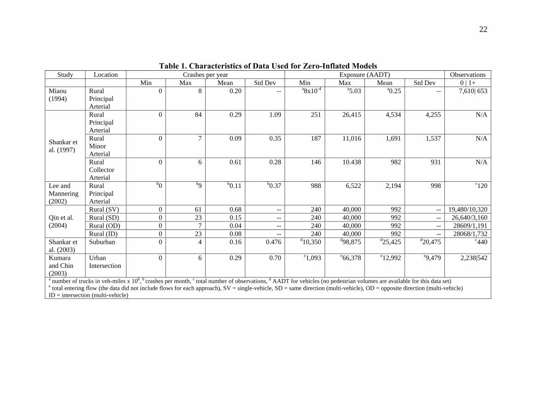
each observation has the same mean λ . Two different types of regression or predictive models have been proposed in the literature for handling this type of data. The first type is known as the hurdle model (Cragg, 1971; Mulhully, 1986). This type of model has not been extensively applied in the statistical field and is therefore not the focus of this paper. The reader is referred to Cragg (1971), Mulhully (1986) and Schmidt and Witte (1989) for additional information about hurdle models. The zero-inflated count models (also called zero-altered probability or count models with added zeroes) represent an alternative way to handle data with a preponderance of zeros. Since their formal introduction by Lambert (1992) (who expanded the work of Johnson and Kotz (1968)), the use of these models has grown almost boundlessly and can be found in numerous fields, including traffic safety. For example, these models have been applied in the fields of manufacturing (Lambert, 1992; Li et al., 1999), economics (Green, 1996), epidemiology (Heilbron, 1994), sociology (Land et al., 1996), trip distribution (Terza and Wilson, 1990) and political science (Zorn, 1996) among others. In essence, zero-inflated regression models are characterized by a dual-state process, where the observed count can either be located in a perfect state or in an imperfect state with a mean µ. This type of model is suitable for data generated from two fundamentally different states. As described in Washington et al. (2003), consider the following example. A transportation survey asks how many times you have taken mass transit to work during the past week. An observed zero could arise in two distinct ways. First, last week a respondent may have opted to take the vanpool instead of mass transit. Alternatively, a respondent may never take transit, as a result of other commitments on the way to and from their place of employment, lack of viable transit routes, lack of proximity of transit stations, etc. Thus two states are present, one being a normal count-process state and the other being a zero-count state. The count of zeroes observed across the entire population of respondents under this dual state process results in “excess” zeroes not explained by a Poisson or Negative Binomial process. The reader is referred to Lambert (1992), Li et al. (1999), and Lord et al. (2004) for additional information about the pdf and the characteristics of likelihood function of zero-inflated models. WHAT EMPIRICAL CRASH DATA TELL US This section presents the results of a critical review of the work performed on the application of zero-inflated models in traffic safety. Table 1 summarizes crash data characteristics from six published studies. The table includes the proxy for exposure to risk, statistics on crash counts, and type and location of segments. The mean number of crashes per year is very low for each dataset. This is expected since all the studies have a substantially high number of zeros. Where the information is available, the datasets are shown to have between 2% to 12% more zeros than what would be expected given the mean number of crashes per year and a normal Poisson distribution (column #5). Second, with the exception of the last two studies, all highway segments are classified as arterial or collector roads and are located in a rural area. As discussed in the next paragraph, these types of highways are usually classified as ‘high risk’. Third, the first five datasets

8

are shown to have very low average exposure; this characteristic is confirmed by looking at the right-hand side of Table 1. It is possible that the low exposure may explain the preponderance of zeros in the data. The prevalence of zeros in the last dataset is probably explained by another phenomenon, which is discussed below.

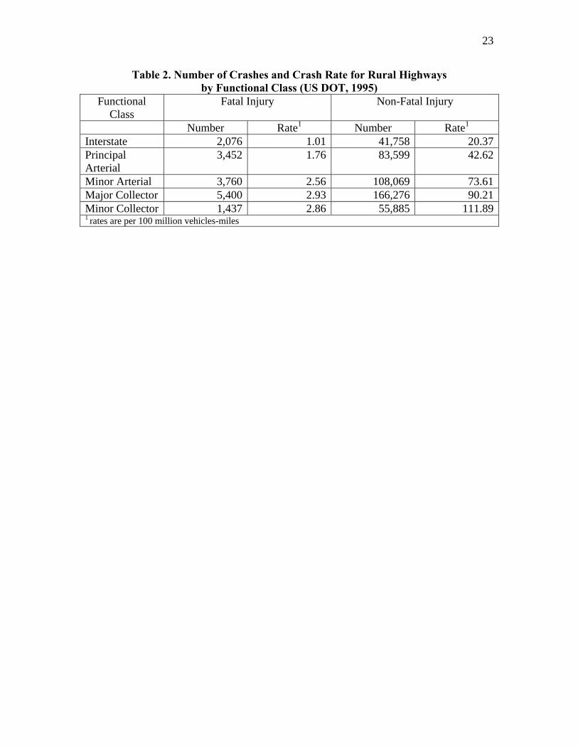
Table 1 here Table 2 summarizes the crash rate by functional class for rural highways in the United States. This table clearly shows that arterial and collector rural segments are more dangerous than interstate highways. In fact, a person is about 5 and 2 times more likely, given the exposure, to be involved in a crash on a minor collector or a principal arterial than a freeway respectively. Other researchers have confirmed the results shown in Table 2. For instance, Amoros et al. (2003) found that rural collector roads are generally about twice as dangerous as rural freeway segments for 8 counties in France. Brown and Baass (1995) evaluated crash rates by severity for different types of highway located within the vicinity of Montreal, Quebec. They reported that a driver is about 2 to 3 times more likely to be involved in a collision on rural principal and arterial roads than on freeways. The crashes were also found to be more severe for principal arterial roads.

Table 2 here The characteristics illustrated in Tables 1 and 2 show interesting, if not counterintuitive results. In a general sense, it is puzzling to note that a typical rural highway that has inherently safe segments would, at the same time, belong to a group classified as the most dangerous type of highways. This observation can be explained in one of two ways: either 1) rural highways include many inherently safe segments and a few tremendously dangerous segments, which results in an overall average crash rate much higher than that of freeway segments, or 2) crashes simply do not follow a dual-state process, but a single process characterized by low exposure. Another point worth mentioning is that rural highway segments characterized by high exposure or traffic volumes have never been found to follow a dual-state process (Hauer and Persaud, 1995; Harwood et al., 2000). Another characteristic detailed in Table 1 concerns the high percentage of zeros (80%) for approaches of signalized 3-legged intersections located in Singapore (Kumara and Chin, 2003). At first glance, this high percentage appears to be counterintuitive, especially since intersection-related crashes usually account for about half of all crashes occurring in urban environments (NHTSA, 2000). In another study, Lord (2000) found that 3-legged signalized intersections in Toronto, Ontario experienced on average 4.8 crashes per year and only 10% of the intersections had zero crashes (all approaches combined). This observation merits further reflection: given the characteristics of each city, their effort placed on improving safety, and the same level of exposure, are 3-legged signalized intersections in Toronto truly three times more dangerous than in Singapore? Perhaps variations in driver behavior and traffic signal design may explain a portion of this difference. However, given that 80% of the approaches had no crashes, the excess zeros at signalized intersections in Singapore are likely attributable to non-reported crashes and perhaps other differences to a lesser degree. Kumara and Chin (2003)

9

acknowledged that the excess zeros could be explained by non-reported crashes. Unfortunately, they did not explore this option further since assuming this prospect would entail that crash data cannot be generated from a dual-state process (see p. 53). Other examples of misconception between an apparent "excess" zeros in crash data and non-reported crashes on rural transportation networks can be found here (Cima International, 2000; Lord et al., 2003a; Lord et al. 2004). SIMULATED CRASH DATA FROM BERNOULLI TRIALS This section presents the results of a simulation study intended to illustrate the concepts discussed in the previous section. In this exercise, a series of simulation runs was performed by replicating a Bernoulli trial with unequal probability of events—the nature of the motor vehicle crash process described previously. A sample of 100 sites was used in the simulation. The individual risk ip was simulated from a combination of uniform and lognormal distributions (e.g., the risk for each site is uniformly distributed and the risk for each driver is lognormal distributed). Data were not generated from a Poisson-Gamma distribution since Poisson Trials, resulting from a Bernoulli trial (with low p and large N) do not follow a standard distribution. In addition, one goal of the simulation effort is to show that the Poisson-Gamma model (the most commonly used) can be used for approximating the motor vehicle crash process; however, this does not imply that it is the best model available. Average individual risk in the simulation varies from about 20 to 111 in 200 million, as detailed in Table 2; these values are similar to what is found elsewhere (see Hauer and Persaud, 1995 or Brown and Baass, 1995). For each site, the estimated mean number of events was computed such that

∑=

==N

iippN

1λ)

(11)

where, λ̂ = the estimated mean number of events in one year;

∑=

=N

iipp

1; and,

N = the number of trials. The simulation was performed using GENSTAT (Payne, 2000) for the following three traffic flow conditions (AADT): 50 vehicles per day, 500 vehicles per day, and 5,000 vehicles per day. Thus, the total number of vehicles in one year is 365 days times AADT. The simulation runs are meant to represent sites with very low exposure, low exposure, and medium exposure to risk respectively. Four series of simulation runs were performed for each of the exposure levels, characterized by the degree of crash risk and the heterogeneity in crash risk (variability in crash risk across different sites).

10

1) high heterogeneity-high risk (Uniform: 0.0001 (Max), 0.00000001 (Min); variance for lognormal: 0.5) 2) low heterogeneity-low risk (Uniform: 0.000001 (Max), 0.00000001 (Min); variance for lognormal: 0.5) 3) very low heterogeneity-medium/high risk (fixed high risk=0.00001; variance for lognomal: 0.5 - all the variance is explained by this distribution) 4) very low heterogeneity-low risk (fixed low risk=0.0000001; variance for lognomal: 0.5 - all the variance is explained by this distribution)

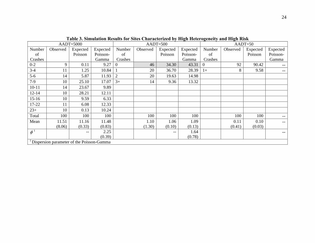
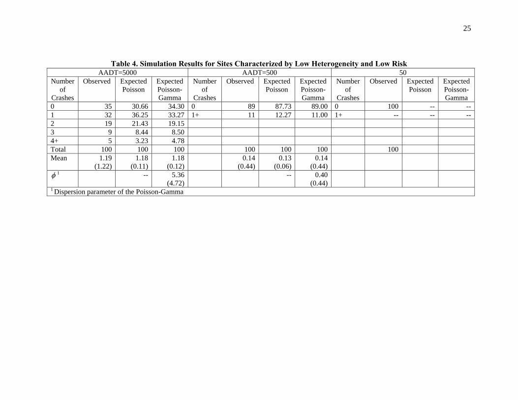
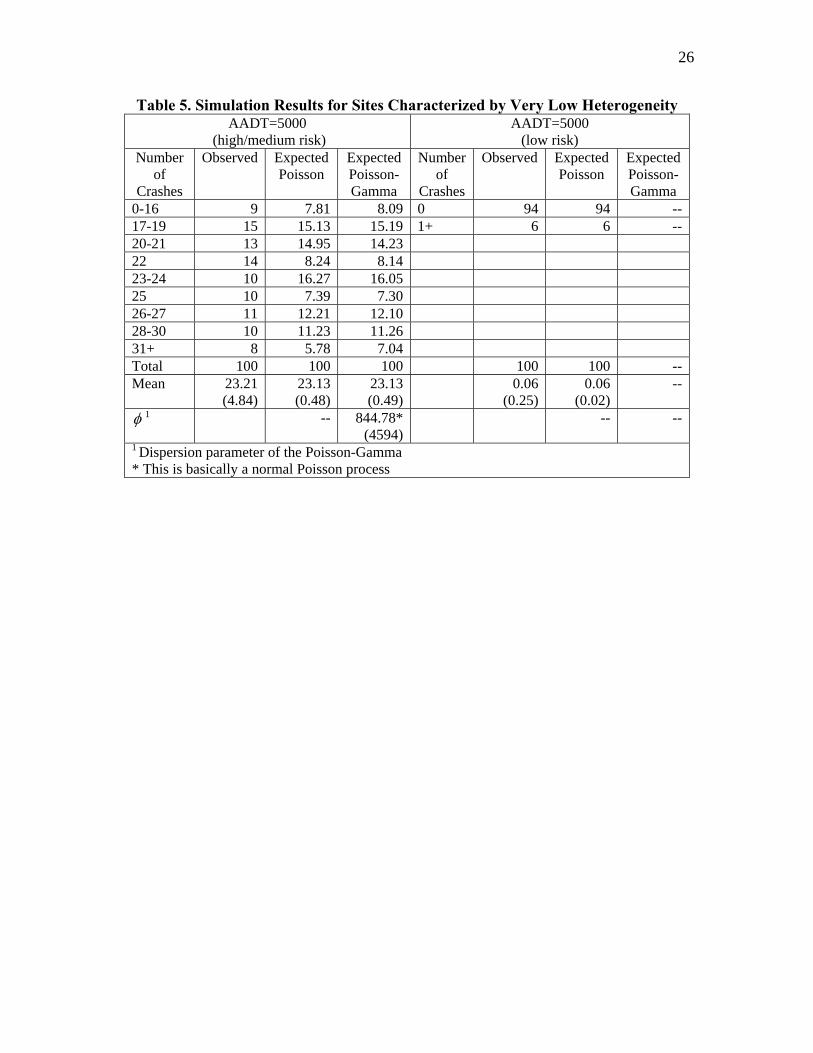
The results of the four simulation runs are presented in Tables 3 through 5. The data shown in theses tables are the fitted frequency distribution estimates, as provided by GENSTAT. Note that the simulation performed in this work is not meant to replicate the actual crash process occurring on transportation networks—the effects of covariates on crashes are important and not assumed, so simplifications have been made. Similarly, all sites used in this exercise are subjected to the same exposure; obviously, it is unreasonable to assume in practice that all sites will have the same exposure. Nonetheless, the simplifications described herein do not hinder conclusions made regarding the simulations. Table 3 summarizes the results of the simulation run used for simulating data with a high degree of heterogeneity and for observations that include sites categorized as high risk. This table shows that the number of events follow a Poisson distribution for sites with very low exposure, with about 92% of the sites having zero crashes. For low exposure, in contrast, the simulation generated more zeros than what would be expected from the Poisson and Poisson-Gamma (NB) distributions. This result seems to agree with the results illustrated in Tables 1 and 2 respectively; sites with a preponderance of zeros are characterized by low exposure and high risk. Finally, despite the fact the data were generated from a Uniform-Lognormal distribution, the Poisson-Gamma (NB) distribution provides a superior statistical fit than the Poisson distribution for sites with medium exposure. Table 4 exhibits the results of the simulation run for low heterogeneity and sites with low risk. The results demonstrate that for low exposure the Poisson distribution offers good statistical fit, although some heterogeneity exits in the data. However, the Poisson-Gamma distribution provides a better fit than the Poisson distribution for medium exposure. Table 4 also reveals that the only situation where a site may be inherently safe is when the exposure tends towards zero, as illustrated in the last columns. Table 5 summarizes the results for sites with very low heterogeneity. The simulation demonstrates that the Poisson distribution can be used to approximate data generated by a nearly homogeneous Bernoulli process. This outcome can clearly be seen both for high and low crash risks.

11

Table 3 here

Table 4 here

Table 5 here DISCUSSION Zero-inflated models have been used in traffic safety studies for modeling crashes for various applications: single- and multi-vehicle crashes on rural two-lane roads (Miaou, 1994; Shankar et al., 1997; Qin et al., 2004); run-off-the-road crashes in rural areas (Lee and Mannering, 2002); crashes occurring at intersections (Mitra, 2002; Kumara and Chin, 2003); and pedestrian crashes taking place on urban and suburban corridors (Shankar et al., 2003). In these studies, the use of the zero-inflated models has often been justified based on their superior statistical fit (almost always centered on the Vuong statistics - see Vuong, 1989). Given the characteristics of these models, these authors have automatically assumed that crashes must follow a dual-state process, with the exception of Miaou (1994) who justified the use of the ZIP not as a dual-state process, but to account for unreported crash data. Although zero-inflated models offer improved statistical fit to crash data in many cases, it is argued in this paper that the inherent assumption of a dual state process underlying the development of these models is inconsistent with crash data. As was shown with both empirical and simulated data, excess observed zeroes arise from low exposure and high risk conditions (this explains the counts at the tail). In addition, the selection of spatial and temporal scales influences the number of observed zeroes. For example, using crashes per 10th of a mile on urban arterials will result in a greater proportion of observed zeroes than using crashes per mile (note: some studies have used small time or space intervals - e.g., Lee and Mannering, 2002). Surely, whether a process is dual state should not rest on the selection of spatial or temporal scale of analysis (see example below). For an inherently safe state to exist, either one of the following two conditions must be present: 1) the probability ip must either be 0 or so low that it approaches 0 for each vehicle that enters the site and/or 2) the number of vehicles N (or exposure) is or tends towards 0 for the given time period under study. Since it unreasonable to assume that each driver (no matter how many) will have a probability ip equal to 0 (a large body of research suggests that crashes are 70% to 90% human error), the number of vehicles or exposure must approach 0 (or be sufficiently small). This outcome is in accordance with both empirical and simulated crash data presented in this paper. The characteristic described in the previous paragraph can be expressed or conceptualized in a dual state framework such that (see equations (9), (10) and (11)):

12

∑=

→==N

iippN

111 0λ

) (12)

∑=

==M

jjppM

122λ

)

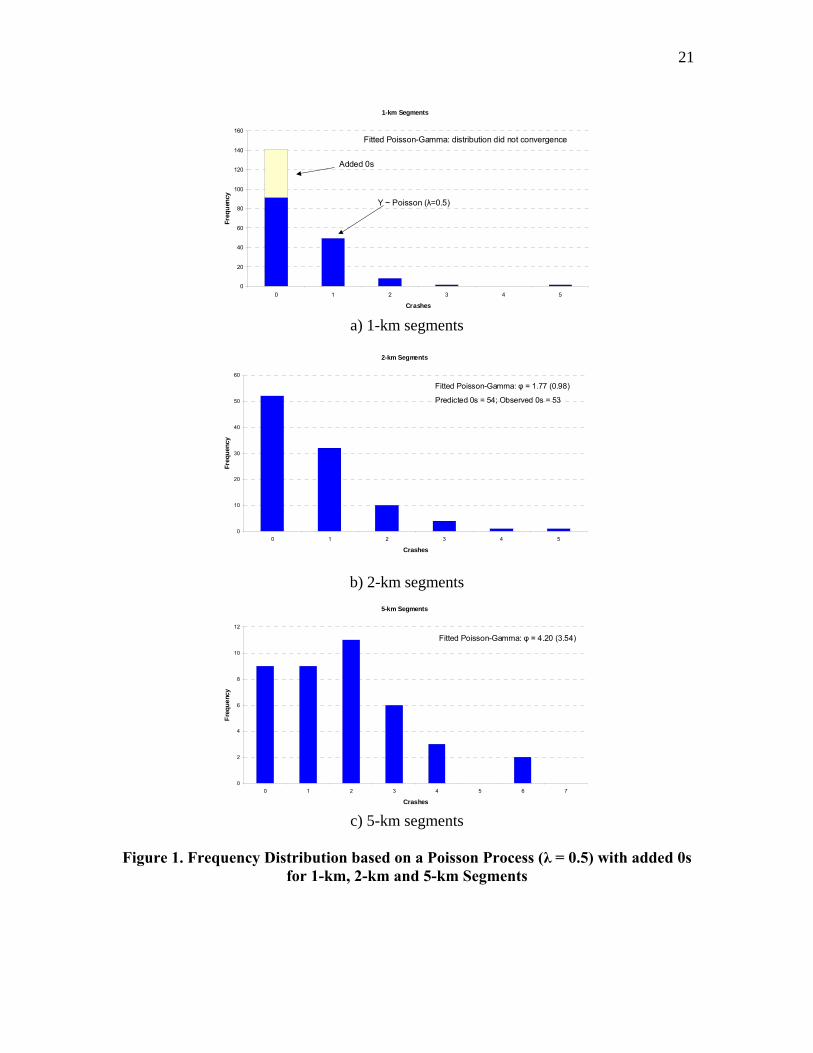
where 1λ is the mean of the first distribution (or state) that tends towards 0; 2λ is the mean of the second distribution; N is the number of vehicles traveling through sites included in the first distribution; and M is the number of vehicles traveling through sites contained of the second distribution. If the second distribution (i.e., for 2λ ) follows a normal Poisson process (such as the ZIP), then every site has theoretically the same mean and the data must meet the properties of equation (5). Furthermore, this attribute entails that each site must automatically have nearly the same exposure (or the same number of vehicles), given the characteristics of equation (5), in order to obtain the same mean. In practice, it is unreasonable to assume that each site will be subjected to the same exposure; thus, violating the properties of equation (5) and the fixed mean across different sites. If the second distribution is characterized by a variance-to-mean ratio above 1 (such as the ZINB), the inequality of equation (6) holds and over-dispersion exists in the second dataset. As explained previously, the use of different space or time scales affects exposure, which in return influences the number of zeros present in the data (note: it will also affect the entire distribution, not just the number of zeros). To demonstrate this characteristic, a simple example is illustrated in Figure 1. In this figure, crashes estimated from a Poisson distribution were simulated with a mean 5.0=λ for 150 sites. This simulation could represent 1-km highway segments with similar characteristics. Then, 50 sites with 0 crash count were added randomly to this distribution to characterize a dual-state process for a total of 200 1-km segments. A Poisson-Gamma distribution could not be fitted adequately to the proposed mixed distribution, confirming that too many zeros exist in the data. Once the simulation was completed, the sections were grouped into 2-km and 5-km segments respectively. As expected, Figure 1 shows that the number of sites with zeroes diminishes drastically with longer segments. In fact, even with 2-km segments, the over-presentation of zeros disappears (i.e., more zeros than what would be expected given the new estimated mean), as shown with the fitted Poisson-Gamma distribution in Figure 1b. Although this example focused on the space scale, the same results would be observed when different time scales are used (e.g., crashes per 5 years versus crashes per 5 minutes for the same segment length, etc.).

Figure 1 here If ZIP and ZINB models provide good statistical fit but do not characterize the underlying crash process, several interesting questions arise. First, what are the consequences of applying these models? Second, what alternative models should be used instead? Answers to these two questions are now provided.

13

If the only goal consists of finding the best statistical fit then the zero-inflated models may be appropriate, since they offer improved statistical fit compared to Poisson or Poisson-Gamma models. However, this may not be sound practice. It can be shown that other types of models provide better fit (i.e., likelihood, MSE, etc.) than Poisson-Gamma models, and some even better than ZIP or ZINB models. For instance, one could use the multilogit-Poisson for modeling multi-state processes. For this type of model, the crash process could be divided into " m " states, representing categories of perfect safety, above average safety, average safety, less than average safety, and least safe. The Multinomial-Poisson process is another modeling approach that will fit the data better than Poisson-Gamma models. The main characteristic of this model is that each count iY follows a multinomial distribution (Dalal et al., 1990; Lang, 2002). Although this type of model provides good statistical fit, it is not commonly used in practice since the likelihood function can be very difficult to compute (Baker, 1994). The ultimate statistical fit can be found using non-parametric (including spline functions) or semi-parametric models (Ullah, 1989; Efromovich, 2000). These models will fit the data better than any parametric model. Their advantage: there is no longer any assumption about whether the data follow any statistical distribution, both for the functional form and the error distribution. The disadvantage is that much faith is lost in agreement with theoretical knowledge of crashes and that any dataset will be grossly overfit by the model and results will not be transferable or generalizable to other locations. Usually what is sought besides good statistical fit is insight into the underlying data generating process—motor vehicle crashes in this study. At risk when using zero-inflated models is the possibility that mis-interpretations about safe and unsafe intersections/road segments/etc. will result. Someone might falsely believe that certain engineering investments—as predicted by the zero-inflated models—will lead to inherently safe locations. The resulting models will be difficult, if not impossible, to interpret in the ‘real world’ of crash causation. It may also lead modelers down the path of finding the best fit to data, possibly over-fitting the models. As stated in Washington et al. (2003), “If there is not a compelling reason to suspect that two states might be present, the use of a zero-inflated model may be simply capturing model mis-specification that could result from factors such as unobserved effects (heterogeneity) in the data.” Examples of commonly omitted variables include non-reporting of crashes, driver distractions, driver competence, etc. The set of variables commonly omitted from crash models may also contribute to explaining the ‘excessive’ zeroes observed in motor vehicle crash data. How then, should crashes be modeled appropriately? The answer derives from revisiting the root of excess zeroes, which are caused by the following four issues: (1) spatial or time scales that are too small; (2) under or mis-reporting of crashes; (3) sites characterized by low exposure and high risk; and (4) important omitted variables describing the crash process. An obvious fix for (1) is to select appropriate time and spatial scales, which in some cases will result in more costly data collection. The remedies for (2), (3), and (4) require modeling solutions. One solution is to estimate NB and Poisson models with a term added to capture unobserved heterogeneity effects. This could account for under- or mis-reporting of crashes and omitted important variables in the crash process, and will yield a fit similar to zero-inflated models.

14

In addition, there exist other statistical tools that can be used for modeling data with a preponderance of zeros commonly observed in crash data. Recall that the excess zeroes are mainly attributed to low exposure (given the time-scale defined as crashes per year) and high risk. Small area statistics (SAS) (also known as small area estimation or SAE) are such tools that can be used for data characterized by low exposure. These tools originated from researchers in survey sciences who frequently deal with small sample sizes (some even have a sample size of zero) (Rao, 2003). Typically, the term "small area" is usually employed for areas where direct estimates of adequate precision cannot be produced. Thus, the goal of SAS is to use "indirect" estimators that "borrow strength" by using values from related areas and/or time periods to increase the "effective" sample size of interest. Empirical and Hierarchical Bayes methods combined with random-effect models are used to model this effect (Hauer, 1997; Carlin and Louis, 2000; Miaou and Lord, 2003). As opposed to zero-inflated models, SAS offer a much better and more rational modeling approach for conducting safety analyses for sites with low exposure. The reader is referred to Ghosh et al. (1998), Mukhopadhyay (1998) and Rao (2003) for additional information on these model types. CONCLUSIONS The objective of this study was to provide defensible guidance on how to appropriate model crash data. The paper was motivated by the vast array of modeling choices, the lack of formal guidance for selecting appropriate statistical tools, and the peculiar nature of crash data, which has lead to lack of consensus among transportation safety modelers. Four main conclusions are drawn from this research. 1. Crash data are best characterized as Bernoulli trials with independence among crashes

and unequal crash probabilities across drivers, vehicles, roadways, and environmental conditions. Because of the small probability of a crash and the large number of trails these Bernoulli trails can be well approximated as Poisson trials.

2. Poisson and Negative Binomial models serve as statistical approximations to the crash process. Poisson models serve well under nearly homogenous conditions, while Negative Binomial models serve better in other conditions.

3. Crash data characterized by a preponderance of zeros is not indicative of an underlying dual-state process. One or more of four conditions lead to excess zeroes in crash data. 1) Sites with a combination of low exposure, high heterogeneity, and sites categorized as high risk; 2) Analyses conducted with small time or spatial scales; 3) Data with a relatively high percentage of missing or mis-reported crashes; and 4) Crash models with omitted important variables.

4. Theoretically defensible solutions for modeling crash data with excess zeroes include changing the spatial or time scale of analysis, including unobserved heterogeneity terms in NB and Poisson models, improving the set of explanatory variables, and applying small area statistical methods.

15

The intent of this paper was to foster new thinking about how to approach the modeling of crash data. A bottom up focus on the crash process has been lacking, and it is hoped that this paper begins to fill this gap in the literature. It may be preferable to begin to develop models that consider the fundamental process of a crash and avoid striving for “best fit” models in isolation. Further work should concentrate on modeling Bernoulli trials with unequal probability of events. In the end, it may be possible to estimate the individual probability of crash risk for different time periods and driving conditions. ACKNOWLEDGEMENTS The authors would like to express their greatest gratitude to Prof. A.D. Barbour for providing additional information about the Poisson approximation, reviewing our work for the mathematical content and providing suggestions to improve the clarity of the discussion for the section on the theoretical principles of motor vehicle crashes. They also thank Dr. Xiao Qin from the Maricopa Association of Governments for his assistance in obtaining additional information about the crash data on rural two-lane roads in Connecticut. This paper benefited from the input of Drs. Jake Kononov, Ezra Hauer, Per E. Gårder, Fred L. Mannering, and two anonymous referees. Their comments and suggestions were greatly appreciated. REFERENCES Abbess, C., Jarett, D., Wright, C.C., 1981. Accidents at Blackspots: estimating the Effectiveness of Remedial Treatment, With Special Reference to the "Regression-to-Mean" Effect. Traffic Engineering and Control 22 (10), pp. 535-542. Amoros, E., Martin, J.L., Laumon, B., 2003. Comparison of Road Crashes Incidence and Severity Between some French Counties. Accident Analysis & Prevention 35 (4), pp. 349-161. Barbour, A.D., Holst, L., Janson, S., 1992. Poisson Approximation. Clarendon Press, New York, New York. Baker, S.G., 1994. The Multinomial-Poisson Transformation. The Statistician 43 (4), pp. 495-504. Brown, B., Baass, K.A., 1995. Projet d’identification des sites dangereux sur les routes numérotées en Montérégie. Vol 1 : Synthèse. Direction de la santé publique. St-Hubert, Quebec. (In French) Cameron, A.C., Trivedi, P.K. 1998. Regression Analysis of Count Data. Cambridge University Press, Cambridge, U.K.

16

CIMA International, 2000. Étude relative à l’élaboration d’un plan d’actions en matière de sécurité routière en milieu interurbain au Burkina Faso. Final Report. Laval, Québec, 2000. (in French) Carlin, B.P., Louis, T.A., 2000. Bayes and Empirical Bayes Methods for Data Analysis. CRC Press, Chapman & Hall, London, U.K. Cohen, A.C., 1963. Estimation in Mixtures of Discrete Distributions. In Proceedings of the International Symposium on Discrete Distributions, Montreal, Quebec. Cragg, J.G., 1971. Some Statistical Models for Limited Dependent Variables with Application to the Demand for Durable Goods. Econometrica 39, pp. 829-844. Dalal, S.R., Lee, J.C., Sabaval, D.J., 1990. Empirical Bayes Prediction for Compound Poisson-Multinomial Process. Statistic & Probability Letters 9, pp. 385-389. Drezner, Z., Farnum, N., 1993. A Generalized Binomial Distribution. Communication in Statistics: Theory and Methods 22 (11), pp. 3051-3063. Efromovich, S., 1999. Nonparametric curve estimation: methods, theory and applications. Springer, New York, N.Y. Feller, W., 1968. An Introduction to Probability Theory and its Application, Vol. 1, 3rd Ed., John Wiley, New York, New York. Ghosh, M., Natarajan, K., Stroud, T.W.F., Carlin, B.P. 1998. Generalized Linear Models for Small Area Estimation. Journal of the American Statistical Association 93, pp. 273-282. Gourieroux, C.A., Visser, M., 1986. A Count Data Model with Unobserved Heterogeneity. Journal of Econometrics 79, pp. 247-268. Green, W., 1994. Accounting for Excess Zeros and Sample Selection in Poisson and Negative Binomial Regression Models. Working Paper EC-94-10, Department of Economics, Stern School of Business, New York University, New York, N.Y. Harwood, D.W., Council, F.M., Hauer, E., Hughes, W.E., Vogt, A., 2000. Prediction of the Expected Safety Performance of Rural Two-Lane Roads. FHWA-RD-99-207. U.S. Department of Transportation, Washington, D.C. Hauer, E., 1997. Observational Before-After Studies in Road Safety: Estimating the Effect of Highway and Traffic Engineering Measures on Road Safety. Elsevier Science Ltd, Oxford. Hauer, E., 2001. Overdispersion in Modelling Accidents on Road Sections and in Empirical Bayes Estimation. Accident Analysis & Prevention 33 (6), pp. 799-808.

17

Hauer, E., Ng, J.C.N., Lovell, J. 1988. Estimation of Safety at Signalized Intersections. Transportation Research Record 1185, pp. 48-61. Hauer, E., Persaud, B.P., 1995. Safety Analysis of Roadway Geometric and Ancillary Features. Research Report for the Transportation Association of Canada, Ottawa, Canada. Heilbron, D.C., 1994. Zero-Altered and Other Regression Models for Count Data with Added Zeros. Journal of Biometrics 5, pp. 531-547. Ivan, J.N., Wang, C., Bernardo, N.R., 2000. Explaining Two-Lane Highway Crash Rates Using Land Use and Hourly Exposure. Accident Analysis & Prevention 32 (6), pp. 787-795. Johnson, N.L., Kotz, S., 1968. Discrete Distributions: Distributions in Statistics. John Wiley & Sons, New York, N.Y. Kononov, J., Janson, B.N., 2002. Diagnostic Methodology for Detection of Safety Problems at Intersections. Transportation Research Record 1784, pp. 51-56. Kulmala, R., 1995. Safety at Rural Three- and Four-Arm Junctions: Development and Applications of Accident Prediction Models. VTT Publications 233, Technical Research Centre of Finland, Espoo. Kumara, S.S.P., Chin, H.C., 2003. Modeling Accident Occurrence at Signalized Tee Intersections with Special Emphasis on Excess Zeros. Traffic Injury Prevention 3 (4), pp. 53-57. Lambert, D., 1992. Zero-Inflated Poisson Regression, With an Application to Defects in Manufacturing. Technometrics 34 (1), pp. 1-14. Land, K.C., McCall, P.L., Nagin, D.S., 1996. A Comparison of Poisson, Negative Binomial, Semiparametric Mixed Poisson Regression Models, With Empirical Applications to Criminal Careers Data. Sociological Methods & Research 24 (4), pp. 387-442. Lang, J.B., 2002. Multinomial-Poisson Homogeneous and Homogeneous Linear Predictor Models: A Brief Description. online html document: http://www.stat.uiowa.edu/~jblang/mph.fitting/mph.fit.documentation.htm. Accessed on February 11th, 2004. Lee, J., Mannering, F.L., 2002. Impact of Roadside Features on the Frequency and Severity of Run-Off-Road Accidents: An Empirical Analysis. Accident Analysis & Prevention 34 (2), pp. 349-161.

18

Li, C.-C., Lu, J.-C., Park, J., Kim, K., Brinkley, P.A., Peterson, J.P., 1999. Multivariate Zero-Inflated Poisson Models and Their Applications. Technometrics 41 (1), pp. 29-38. Loader, C., 1999. Local Regression and Likelihood. Springer-Verlag, New York, N.Y. Lord, D., 2000. The Prediction of Accidents on Digital Networks: Characteristics and Issues Related to the Application of Accident Prediction Models. Ph.D. Dissertation, Department of Civil Engineering, University of Toronto, Toronto. Lord, D., Abdou, H.A., N'Zué, A., Dionne, G., Laberge-Nadeau, C., 2003a. Traffic Safety Diagnostic and Application of Countermeasures for Rural Roads in Burkina Faso. Transportation Research Record 1846, pp. 39-43. Lord, D., Abdou, H.A., N'Zué, A., Dionne, G., Laberge-Nadeau, C., 2003b. Investigating Sites located on Rural Two-Lane Roads in Burkina Faso for Safety Improvement. Working Paper, Texas Transportation Institute, College Station, TX. Lord, D., Persaud, B.N., 2000. Accident Prediction Models with and without Trend: Application of the Generalized Estimating Equations Procedure. Transportation Research Record 1717, 102-108. Lord, D., Washington, S.P., Ivan, J.N., 2004. Statistical Challenges with Modeling Motor Vehicle Crashes: Understanding the Implications of Alternative Approaches. Research Report CTS-04_01, Texas Transportation Institute, College Station, Texas. (available at http://tti.tamu.edu/product/catalog/reports/CTS-04_01.pdf) (also presented at the 83rd Annual Meeting of the Transportation Research Board, Washington, D.C.) Lyon, C., Oh, J., Persaud, B.N., Washington, S.P., Bared, J., 2003. Empirical Investigation of the IHSDM Accident Prediction Algorithm for Rural Intersections. Transportation Research Record 1840. pp. 78-86. Miaou, S.-P., 1994. The Relationship Between Truck Accidents and Geometric Design of Road Sections: Poisson versus Negative Binomial Regressions. Accident Analysis & Prevention 26 (4), pp. 471-482. Miaou, S.-P., Lord, D., 2003. Modeling Traffic Crash-Flow Relationships for Intersections: Dispersion Parameter, Functional Form, and Bayes versus Empirical Bayes. Transportation Research Record 1840, pp. 31-40. Mitra, S., Chin, H.C., Quddus, M.A., 2002. Study of Intersection Accident by Maneuvre Type. Transportation Research Record 1784, pp. 43-50. Mukhopadhyay, P., 1998. Small Area Estimation in Survey Sampling. Nasora Publishing House, New Delhi.

19

Mullahy, J., 1986. Specification and Testing of Some Modified Count Data Models. Journal of Econometrics 33, pp. 341-365. Neldelman, J., Wallenius, T., 1986. Bernoulli Trials, Poisson Trials, Surprising Variance, and Jensen's Inequality. The American Statistician 40 (4), pp. 286-289. NHTSA, 2000. Traffic Safety Facts: 1999. U.S. Department of Transportation, Washington, D.C. Payne, R.W. (ed.), 2000. The Guide to Genstat. Lawes Agricultural Trust, Rothamsted Experimental Station, Oxford, U.K. Oh, J., Lyon, C., Washington, S.P., Persaud, B.N., Bared, J., 2003. Validation of the FHWA Crash Models for Rural Intersections: Lessons Learned. Transportation Research Record 1840. pp 41-49. Olkin, I., Gleser, L.J., Derman, C., 1980. Probability Models and Applications. MacMillan Publishing Co., Inc., New York, N.Y. Persaud, B.N., Dzbik, L., 1993. Accident Prediction Models for Freeways. Transportation Research Record 1401, pp. 55-60. Poch, M., Mannering, F.L., 1996. Negative Binomial Analysis Of Intersection-Accident Frequency. Journal of Transportation Engineering, Vol. 122, No. 2, 105-113. Poormeta, K., 1999. On the Modelling of Overdispersion of Counts. Statistica Neerlandica 53 (1), pp. 5-20. Rao, J.N.K., 2003. Small Area Estimation. A John Wiley & Sons, Inc. Hoboken, N.J. Rider, P.R., 1961. Estimating the Parameters of Mixed Poisson, Binomial and Weibull Distributions by Method of Moments. Bulletin de l'Institut International de Statistiques 38, Part 2. Qin, X., Ivan, J.N., Ravishankar, N., 2004. Selecting Exposure Measures in Crash Rate Prediction for Two-Lane Highway Segments. Accident Analysis & Prevention 36 (2), pp. 183-191. Shankar, V., Milton, J., Mannering, F.L., 1997. Modeling Accident Frequency as Zero-Altered Probability Processes: An Empirical Inquiry. Accident Analysis & Prevention, Vol. 29, No. 6, pp. 829-837. Shankar, V.N., Ulfarsson, G.F., Pendyala, R.M., Nebergal, M.B., 2003. Modeling Crashes Involving Pedestrians and Motorized Traffic. Safety Science, Vol. 41, No. 7, pp. 627-640.

20

Schmidt, P., Witte, A., 1989. Predicting Criminal Recidivism Using Split-Population Survival Time Models. Journal of Econometrics 40, pp. 141-159. Taylor, L.R., 1961. Aggregation, Variance, and the Mean. Nature, Vol. 189, pp. 732-735. Terza, J.V., Wilson, P., 1990. Analyzing Frequencies of Several Types of Events: A Mixed Multinomial-Poisson Approach. Review of Economics and Statistics, 72 (2), pp. 108-115. Ullah, A., 1989. Semiparametric and nonparametric econometrics. Physica-Verlag, New York, N.Y. US DOT, 1995. Highway Safety Performance - 1992: Fatal and Injury Accident Rates on Public Roads in the United States. Federal Highway Administration, Washington, D.C. Vellaisamy, P., Punnen, A.P., 2001. On the Nature of the Binomial Distribution. Journal of Applied Probability 38 (1), pp. 36-44. Vuong, Q.H., 1989. Likelihood Ratio Tests for Model Selection and Non-Nested Hypothesis. Econometrica 57, pp. 307-333. Washington, S.P., Karlaftis, M., Mannering, F.L., 2003. Statistical and Econometric Methods for Transportation Data Analysis. Chapman and Hall, Boca Raton. Zorn, C.J.W., 1996. Evaluating Zero-Inflated and Hurdle Poisson Specifications. Working Paper. Department of Political Science, Ohio State University, Columbus, OH. Yoneda, K., 1962. Estimations in Some Modified Poisson Distributions. Yokohama Mathematical Journal 10, pp. 73-96.

21

a) 1-km segments

b) 2-km segments

c) 5-km segments Figure 1. Frequency Distribution based on a Poisson Process (λ = 0.5) with added 0s

for 1-km, 2-km and 5-km Segments

1-km Segments

0

20

40

60

80

100

120

140

160

0 1 2 3 4 5

Crashes

Freq

uenc

y

Fitted Poisson-Gamma: distribution did not convergence

Added 0s

Y ~ Poisson (λ=0.5)

2-km Segments

0

10

20

30

40

50

60

0 1 2 3 4 5

Crashes

Freq

uenc

y

Fitted Poisson-Gamma: φ = 1.77 (0.98)

Predicted 0s = 54; Observed 0s = 53

5-km Segments

0

2

4

6

8

10

12

0 1 2 3 4 5 6 7

Crashes

Freq

uenc

y

Fitted Poisson-Gamma: φ = 4.20 (3.54)

22

Table 1. Characteristics of Data Used for Zero-Inflated Models Study Location Crashes per year Exposure (AADT) Observations

Min Max Mean Std Dev Min Max Mean Std Dev 0 | 1+ Miaou (1994)

Rural Principal Arterial

0 8 0.20 -- a8x10-4 a5.03 a0.25 -- 7,610| 653

Rural Principal Arterial

0 84 0.29 1.09 251 26,415 4,534 4,255 N/A

Rural Minor Arterial

0 7 0.09 0.35 187 11,016 1,691 1,537 N/A Shankar et al. (1997)

Rural Collector Arterial

0 6 0.61 0.28 146 10.438 982 931 N/A

Lee and Mannering (2002)

Rural Principal Arterial

b0 b9 b0.11 b0.37 988 6,522 2,194 998 c120

Rural (SV) 0 61 0.68 -- 240 40,000 992 -- 19,480/10,320 Rural (SD) 0 23 0.15 -- 240 40,000 992 -- 26,640/3,160 Rural (OD) 0 7 0.04 -- 240 40,000 992 -- 28609/1,191

Qin et al. (2004)

Rural (ID) 0 23 0.08 -- 240 40,000 992 -- 28068/1,732 Shankar et al. (2003)

Suburban 0 4 0.16 0.476 d10,350 d98,875 d25,425 d20,475 c440

Kumara and Chin (2003)

Urban Intersection

0 6 0.29 0.70 e1,093 e66,378 e12,992 e9,479 2,238|542

a number of trucks in veh-miles x 106, b crashes per month, c total number of observations, d AADT for vehicles (no pedestrian volumes are available for this data set) e total entering flow (the data did not include flows for each approach), SV = single-vehicle, SD = same direction (multi-vehicle), OD = opposite direction (multi-vehicle) ID = intersection (multi-vehicle)

23

Table 2. Number of Crashes and Crash Rate for Rural Highways by Functional Class (US DOT, 1995)

Functional Class

Fatal Injury Non-Fatal Injury

Number Rate1 Number Rate1 Interstate 2,076 1.01 41,758 20.37Principal Arterial

3,452 1.76 83,599 42.62

Minor Arterial 3,760 2.56 108,069 73.61Major Collector 5,400 2.93 166,276 90.21Minor Collector 1,437 2.86 55,885 111.891 rates are per 100 million vehicles-miles

24

Table 3. Simulation Results for Sites Characterized by High Heterogeneity and High Risk AADT=5000 AADT=500 AADT=50

Number of

Crashes

Observed Expected Poisson

Expected Poisson-Gamma

Number of

Crashes

Observed Expected Poisson

Expected Poisson-Gamma

Number of

Crashes

Observed Expected Poisson

Expected Poisson-Gamma

0-2 9 0.11 9.27 0 46 34.30 43.31 0 92 90.42 --3-4 11 1.25 10.84 1 20 36.70 28.39 1+ 8 9.58 --5-6 14 5.87 11.93 2 20 19.63 14.98 7-9 10 25.10 17.07 3+ 14 9.36 13.32 10-11 14 23.67 9.89 12-14 10 28.21 12.11 15-16 10 9.59 6.33 17-22 11 6.08 12.33 23+ 10 0.13 10.24 Total 100 100 100 100 100 100 100 100 --Mean 11.51

(8.06) 11.16 (0.33)

11.48 (0.83)

1.10 (1.30)

1.06 (0.10)

1.09 (0.13)

0.11 (0.41)

0.10 (0.03)

--

φ 1 -- 2.25 (0.39)

-- 1.64 (0.78)

--

1 Dispersion parameter of the Poisson-Gamma

25

Table 4. Simulation Results for Sites Characterized by Low Heterogeneity and Low Risk AADT=5000 AADT=500 50

Number of

Crashes

Observed Expected Poisson

Expected Poisson-Gamma

Number of

Crashes

Observed Expected Poisson

Expected Poisson-Gamma

Number of

Crashes

Observed Expected Poisson

Expected Poisson-Gamma

0 35 30.66 34.30 0 89 87.73 89.00 0 100 -- --1 32 36.25 33.27 1+ 11 12.27 11.00 1+ -- -- --2 19 21.43 19.15 3 9 8.44 8.50 4+ 5 3.23 4.78 Total 100 100 100 100 100 100 100Mean 1.19

(1.22) 1.18

(0.11) 1.18

(0.12) 0.14

(0.44)0.13

(0.06)0.14

(0.44)

φ 1 -- 5.36 (4.72)

-- 0.40 (0.44)

1 Dispersion parameter of the Poisson-Gamma

26

Table 5. Simulation Results for Sites Characterized by Very Low Heterogeneity AADT=5000

(high/medium risk) AADT=5000

(low risk) Number

of Crashes

Observed Expected Poisson

Expected Poisson-Gamma

Number of

Crashes

Observed Expected Poisson

Expected Poisson-Gamma

0-16 9 7.81 8.09 0 94 94 --17-19 15 15.13 15.19 1+ 6 6 --20-21 13 14.95 14.23 22 14 8.24 8.14 23-24 10 16.27 16.05 25 10 7.39 7.30 26-27 11 12.21 12.10 28-30 10 11.23 11.26 31+ 8 5.78 7.04 Total 100 100 100 100 100 --Mean 23.21

(4.84) 23.13 (0.48)

23.13 (0.49)

0.06 (0.25)

0.06 (0.02)

--

φ 1 -- 844.78* (4594)

-- --

1 Dispersion parameter of the Poisson-Gamma * This is basically a normal Poisson process