inference for zero-inflated poisson...
TRANSCRIPT
41
Chapter 3
Inference for Zero-Inflated Poisson Distribution
3.0 Introduction
In chapter two, we have discussed inference for θ of Zero-Inflated
Power Series Distribution. Zero-Inflated Poisson Distribution is a particular
case of Zero-Inflated Power Series Distribution. In this chapter, we provide
the inference for Zero-Inflated Poisson Distribution and Zero-Inflated
Truncated Poisson Distribution. In the literature, numbers of researchers have
worked on zero-inflated Poisson distribution. Yip (1988) has described an
inflated Poisson distribution dealing with the number of insects per leaf.
Lambert (1992) considered zero-inflated Poisson regression model. Van Den
Broek (1995) has discussed score test for testing Poisson distribution against
ZIP distribution. Xie et al. (2001) have reported use of ZIP distribution in
statistical process control and studied performance of various tests for testing
Poisson distribution against zero-inflated Poisson alternative. Gupta et al.
(2004) have discussed score test for zero-inflated generalized Poisson
regression model. Thas et al. (2005) have discussed smooth tests for the zero-

42
inflated Poisson distribution. Castillo et al. (2005) have studied overdispersed
and underdispersed Poisson distributions.
ZIPD contains two parameters. The first parameter )(π indicates
inflation of zero and the other parameter )(θ is that of Poisson distribution. In
this chapter, we focus on the inference of parameter θ of ZIPD. However it
appears that no test has been reported for testing parameter θ of Poisson
distribution. We provide maximum likelihood estimators, Fisher information
matrix and moment estimator of the parameters. The three asymptotic tests for
testing the parameter of Poisson distribution based on full likelihood,
conditional likelihood and moment estimator are provided. The performance
of these three tests has been studied for ZIPD. Asymptotic confidence
intervals for the parameter are also provided.
The rest of the chapter is organized as follows. In section 3.1, we
report maximum likelihood estimators of both the parameters of ZIPSD and
corresponding asymptotic variances using full likelihood and conditional
likelihood approach. In section 3.2, we provide three asymptotic tests for
testing the parameter of Poisson distribution. In section 3.3, the performance
of the three tests has been studied by simulation. We have developed C -
program for the same (Appendix 1). Based on study it is observed that an
asymptotic test based on full likelihood estimator and the one based on
conditional likelihood estimator have nearly similar performance. In section
3.4, the asymptotic confidence intervals based on three estimation approaches
are given. Section 3.5 is devoted to ZITPD. The ZITPD is a member of
ZIPSD. All the theory is analogues to ZIPD. Section 3.6 devoted to three tests
for testing the parameters of ZITPD.
3.1 Zero-Inflated Poisson Distribution
Full Likelihood Function Approach
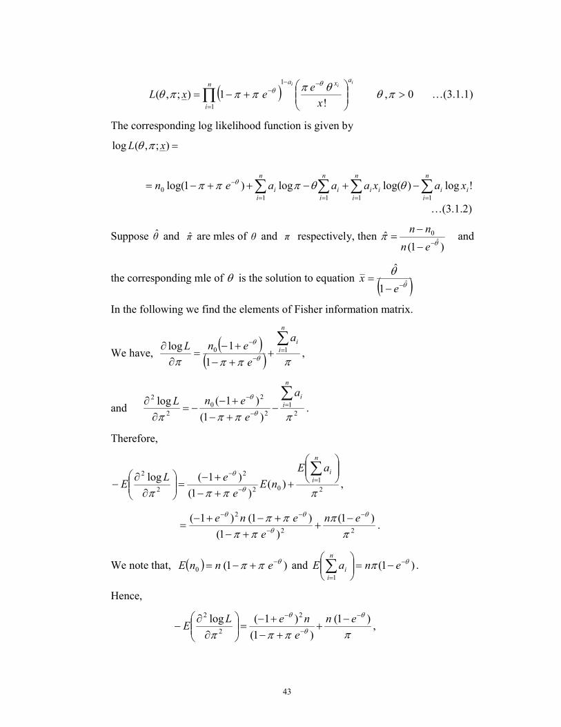
Let nXXX ...,,, 21 be a random sample observed from ZIP distribution, then
the likelihood function is given by
43
( ) 0,!
1);,(
1
1
>
+−=
−−
=
−∏ πθθπ
πππθθ
θi
iia
xan
i x
eexL …(3.1.1)
The corresponding log likelihood function is given by
=);,(log xL πθ
∑∑ ∑∑== ==
− −+−++−=n
i
ii
n
i
n
i
ii
n
i
ii xaxaaaen11 11
0 !log)log(log)1log( θθπππ θ
…(3.1.2)
Suppose θ̂ and π̂ are mles of θ and π respectively, then )1(
ˆˆ
0
θπ
−−
−=
en
nn and
the corresponding mle of θ is the solution to equation ( )θθ
ˆ1
ˆ
−−=
ex
In the following we find the elements of Fisher information matrix.
We have, ( )
( ) ππππ θ
θ ∑=
−
−
++−
+−=
∂∂
n
i
ia
e
enL 10
1
1log,
and 2
1
2
20
2
2
)1(
)1(log
ππππ θ
θ ∑=
−
−
−+−
+−−=
∂
∂
n
i
ia
e
enL.
Therefore,
2
1
02
2
2
2
)()1(
)1(log
ππππ θ
θ
++−
+−=
∂
∂−
∑=
−
−
n
i
iaE
nEe
eLE ,
22
2 )1(
)1(
)1()1(
ππ
ππππ θ
θ
θθ −
−
−− −+
+−
+−+−=
en
e
ene.
We note that, ( ) )1(0
θππ −+−= ennE and )1(1
θπ −
=
−=
∑ enaE
n
i
i .
Hence,
ππππ
θ
θ
θ )1(
)1(
)1(log 2
2
2 −
−
− −+
+−
+−=
∂
∂−
en
e
neLE ,
44
)1(
)1(θ
θ
πππ −
−
+−
−=
e
en. …(3.1.3)
Now
θπππ
θ θ
θ ∑∑ =
=−
−
+−+−
−=∂∂
n
i
iin
i
i
xa
ae
enL 1
1
0
)1(
)(log
2
1
2
0
2
2
)1(
)1(log
θππππ
θ θ
θ ∑=
−
−
−+−
−−=
∂
∂
n
i
ii xa
e
enL
Therefore,
+
+−
−=
∂
∂−
−
−
θπππ
πθ θ
θ 1
)1(
)1(log2
2
e
en
LE …(3.1.4)
Further, ( )2
02
1
log
θ
θ
ππθπ −
−
+−−=
∂∂∂
e
enL
Hence
( )θθ
ππθπ −
−
+−=
∂∂∂
−e
enLE
1
log2
…(3.1.5)
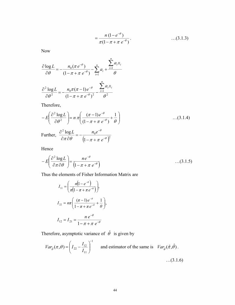
Thus the elements of Fisher Information Matrix are
( )
( )
+−−
=−
−
θ
θ
eπππ
enI
1
111 ,
+
+−
−=
−
−
θeππ
eππnI
θ
θ1
1
)1(22 ,
θ
θ
ππ −
−
+−==
e
enII
12112
Therefore, asymptotic variance of θ̂ is given by
1
11
1222ˆ ),(
−
−=
I
IIVar θπ
θ and estimator of the same is )ˆ,ˆ(ˆ θπ
θVar .
…(3.1.6)
45
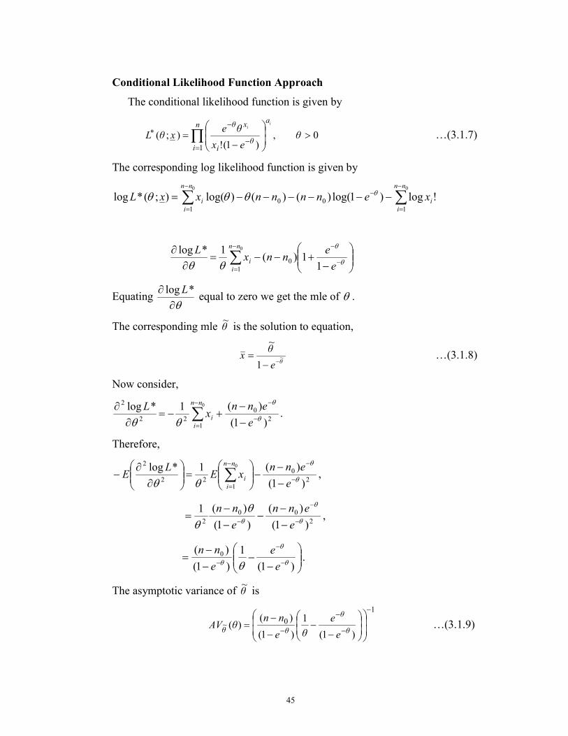
Conditional Likelihood Function Approach
The conditional likelihood function is given by
0,)1(!
);(1
>
−=∏=
−
−∗ θ
ex
θexθL
n
i
a
θi
xθ ii
…(3.1.7)
The corresponding log likelihood function is given by
∑∑−
=
−−
=
−−−−−−=00
1
00
1
!log)1log()()()log();(*lognn
i
i
nn
i
i xennnnxxL θθθθ
−+−−=
∂∂
−
−−
=∑ θ
θ
θθ e
ennx
L nn
i
i1
1)(1*log
0
1
0
Equating θ∂
∂ *log L equal to zero we get the mle of θ .
The corresponding mle θ~
is the solution to equation,
θ
e
θx ~
1
~
−−= …(3.1.8)
Now consider,
2
0
122
2
)1(
)(1*log 0
θ
θ
θθ −
−−
= −
−+−=
∂
∂∑
e
ennx
L nn
i
i .
Therefore,
2
0
122
2
)1(
)(1*log 0
θ
θ
θθ −
−−
= −
−−
=
∂
∂− ∑
e
ennxE
LE
nn
i
i ,
2
00
2 )1(
)(
)1(
)(1θ
θ
θ
θθ −
−
− −
−−
−
−=
e
enn
e
nn,
−−
−
−=
−
−
− )1(
1
)1(
)( 0
θ
θ
θ θ e
e
e
nn.
The asymptotic variance of θ~
is
1
0~
)1(
1
)1(
)()(
−
−
−
−
−−
−
−=
θ
θ
θθe
e
θe
nnθAV …(3.1.9)

46
Moment Estimator of ZIP Distribution
For the zero-inflated Poisson distribution the mean and variance are
given by, θπ== XXE )( and ( ))1(1)( 2 πθπθ −+== SXVar …(3.1.10)
Therefore,
θπ=)(XE and ( )
),()1(1
)( 2 θπσπθπθ=
−+=
nXVar say …(3.1.11)
Let θπ== XXE )( …(3.1.12)
and ( ))1(12 πθπθ −+=S
( )πθθπθ −+= 1
( )XX −+= θ1
2XXX −+= θ
22XXSX +−=θ
X
XXS 22
ˆ +−=θ
)1(ˆ2
XX
S−−=θ
Now, θ
πˆ
ˆX=
Hence, )1(
ˆ2
2
XXS
X
−−=π
22
2
XXS
X
+−= …(3.1.13)
Solving Eq. (3.1.12) and Eq. (3.1.13) we get the moment estimators of π and
θ .
3.2 Tests for the Parameter θ of ZIP Distribution
Let us consider the problem of testing 00 : θθ =H . We assume that π is
unknown.
a) Test Based On θ̂
The test statistic for testing 00 : θθ =H vs 01 : θθ ≠H , is given by
47
),ˆ(
ˆ
00ˆ
07
θπ
θθ
θAV
Z−
= , …(3.2.1)
where )( 0ˆ θθAV is an estimate of asymptotic variance of θ̂ . The test 7ψ
rejects 0H , if 2/17 α−> zZ
b) Test Based On θ~
The test statistic here is: )(
~
0~
08
θ
θθ
θAVZ
−= , …(3.2.2)
where )( 0~ θθAV is as defined in Eq. (3.1.9). The test 8ψ rejects 0H if
2/18 α−> zZ .
c) Test Based On Sample Mean
The test statistic is
),ˆ(ˆ
ˆ
00
2
0
0
0
9
θππ
θπ
XAV
Xn
Z−
−
= , …(3.2.3)
where, 0
0ˆθ
πX= ,
Power of the test is given by
),(9θπβψ ( )∑
=
=Φ+Φ−=n
k
kk knPAB0
0 )()ˆ()ˆ(1
where ( )
),(
),ˆ(ˆˆˆ
0
00
2
02/100
θπ
θπθππθπ α
X
X
kAV
AVzB
−+=
−−
,
( )
),(
),ˆ(ˆˆˆ
0
0
2
02/100
θπ
θπθππθπ α
X
X
kAV
AVzA
−−=
−−
and
( ) knkn
k PPknP −−== )1()( 000 , with ( )θππ −+−= eP 10
48
In the following, we report performance of the three tests developed in
the section (3.2), which is based on simulation experiments.
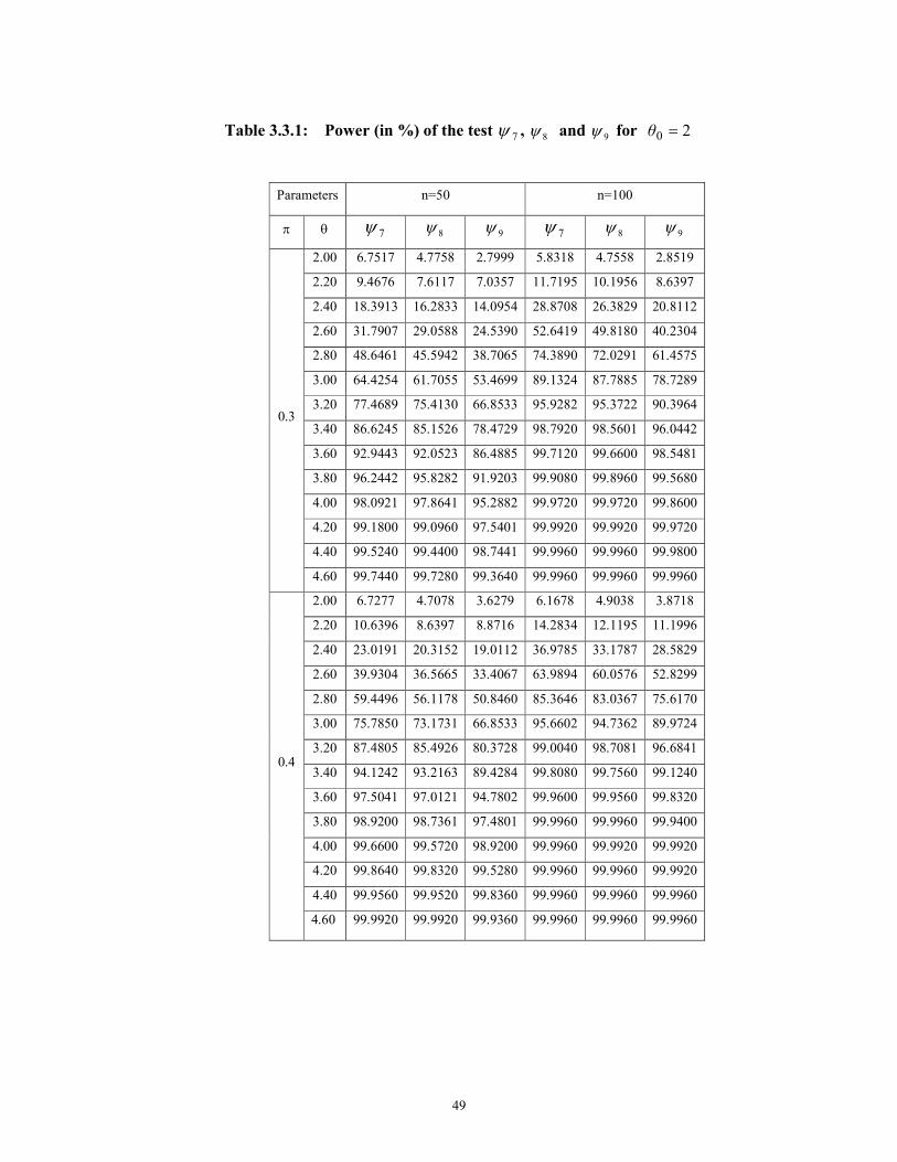
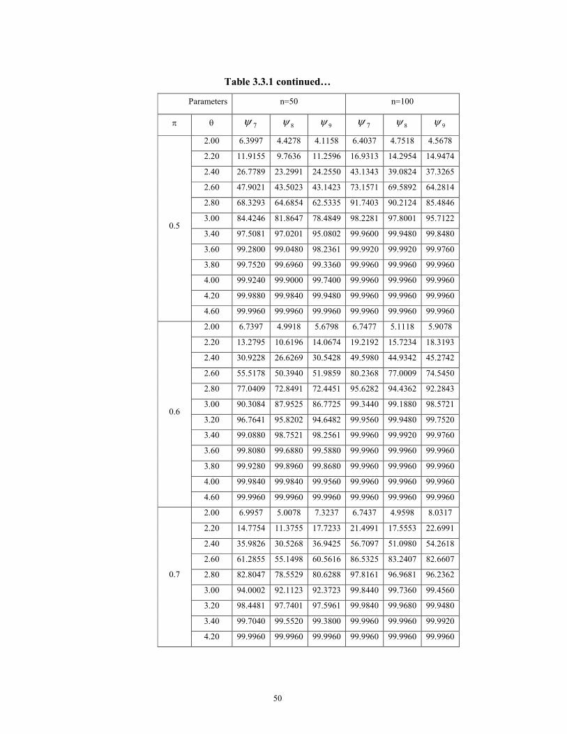
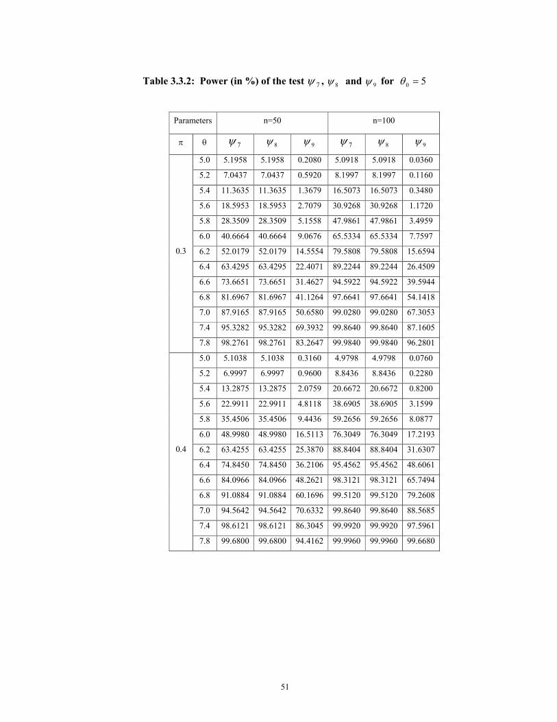
3.3 Simulation Study
A simulation study is carried out to investigate the power of the three
tests proposed in the section 3.2. We generate 25000 samples of sizes 50 and
100 for different values of θ and π . Based on the generated sample, the test
statistics were calculated. Percentage of times the test statistic exceeds 2/1 α−z
is computed. It is infact an estimate of power of the respective test. ‘C’
programs are developed to find power of the test (Appendix 1). The results for
the case of =0θ 2 and 5 and =π 0.3, 0.4, 0.5, 0.6, 0.7 are presented in the
Table 3.3.1 and Table 3.3.2.
49
Table 3.3.1: Power (in %) of the test 7ψ , 8ψ and 9ψ for 20 =θ
Parameters n=50 n=100
π θ 7ψ 8ψ 9ψ 7ψ 8ψ 9ψ
2.00 6.7517 4.7758 2.7999 5.8318 4.7558 2.8519
2.20 9.4676 7.6117 7.0357 11.7195 10.1956 8.6397
2.40 18.3913 16.2833 14.0954 28.8708 26.3829 20.8112
2.60 31.7907 29.0588 24.5390 52.6419 49.8180 40.2304
2.80 48.6461 45.5942 38.7065 74.3890 72.0291 61.4575
3.00 64.4254 61.7055 53.4699 89.1324 87.7885 78.7289
3.20 77.4689 75.4130 66.8533 95.9282 95.3722 90.3964
3.40 86.6245 85.1526 78.4729 98.7920 98.5601 96.0442
3.60 92.9443 92.0523 86.4885 99.7120 99.6600 98.5481
3.80 96.2442 95.8282 91.9203 99.9080 99.8960 99.5680
4.00 98.0921 97.8641 95.2882 99.9720 99.9720 99.8600
4.20 99.1800 99.0960 97.5401 99.9920 99.9920 99.9720
4.40 99.5240 99.4400 98.7441 99.9960 99.9960 99.9800
0.3
4.60 99.7440 99.7280 99.3640 99.9960 99.9960 99.9960
2.00 6.7277 4.7078 3.6279 6.1678 4.9038 3.8718
2.20 10.6396 8.6397 8.8716 14.2834 12.1195 11.1996
2.40 23.0191 20.3152 19.0112 36.9785 33.1787 28.5829
2.60 39.9304 36.5665 33.4067 63.9894 60.0576 52.8299
2.80 59.4496 56.1178 50.8460 85.3646 83.0367 75.6170
3.00 75.7850 73.1731 66.8533 95.6602 94.7362 89.9724
3.20 87.4805 85.4926 80.3728 99.0040 98.7081 96.6841
3.40 94.1242 93.2163 89.4284 99.8080 99.7560 99.1240
3.60 97.5041 97.0121 94.7802 99.9600 99.9560 99.8320
3.80 98.9200 98.7361 97.4801 99.9960 99.9960 99.9400
4.00 99.6600 99.5720 98.9200 99.9960 99.9920 99.9920
4.20 99.8640 99.8320 99.5280 99.9960 99.9960 99.9920
4.40 99.9560 99.9520 99.8360 99.9960 99.9960 99.9960
0.4
4.60 99.9920 99.9920 99.9360 99.9960 99.9960 99.9960
50
Table 3.3.1 continued…
Parameters n=50 n=100
π θ 7ψ 8ψ
9ψ 7ψ 8ψ
9ψ
2.00 6.3997 4.4278 4.1158 6.4037 4.7518 4.5678
2.20 11.9155 9.7636 11.2596 16.9313 14.2954 14.9474
2.40 26.7789 23.2991 24.2550 43.1343 39.0824 37.3265
2.60 47.9021 43.5023 43.1423 73.1571 69.5892 64.2814
2.80 68.3293 64.6854 62.5335 91.7403 90.2124 85.4846
3.00 84.4246 81.8647 78.4849 98.2281 97.8001 95.7122
3.40 97.5081 97.0201 95.0802 99.9600 99.9480 99.8480
3.60 99.2800 99.0480 98.2361 99.9920 99.9920 99.9760
3.80 99.7520 99.6960 99.3360 99.9960 99.9960 99.9960
4.00 99.9240 99.9000 99.7400 99.9960 99.9960 99.9960
4.20 99.9880 99.9840 99.9480 99.9960 99.9960 99.9960
0.5
4.60 99.9960 99.9960 99.9960 99.9960 99.9960 99.9960
2.00 6.7397 4.9918 5.6798 6.7477 5.1118 5.9078
2.20 13.2795 10.6196 14.0674 19.2192 15.7234 18.3193
2.40 30.9228 26.6269 30.5428 49.5980 44.9342 45.2742
2.60 55.5178 50.3940 51.9859 80.2368 77.0009 74.5450
2.80 77.0409 72.8491 72.4451 95.6282 94.4362 92.2843
3.00 90.3084 87.9525 86.7725 99.3440 99.1880 98.5721
3.20 96.7641 95.8202 94.6482 99.9560 99.9480 99.7520
3.40 99.0880 98.7521 98.2561 99.9960 99.9920 99.9760
3.60 99.8080 99.6880 99.5880 99.9960 99.9960 99.9960
3.80 99.9280 99.8960 99.8680 99.9960 99.9960 99.9960
4.00 99.9840 99.9840 99.9560 99.9960 99.9960 99.9960
0.6
4.60 99.9960 99.9960 99.9960 99.9960 99.9960 99.9960
2.00 6.9957 5.0078 7.3237 6.7437 4.9598 8.0317
2.20 14.7754 11.3755 17.7233 21.4991 17.5553 22.6991
2.40 35.9826 30.5268 36.9425 56.7097 51.0980 54.2618
2.60 61.2855 55.1498 60.5616 86.5325 83.2407 82.6607
2.80 82.8047 78.5529 80.6288 97.8161 96.9681 96.2362
3.00 94.0002 92.1123 92.3723 99.8440 99.7360 99.4560
3.20 98.4481 97.7401 97.5961 99.9840 99.9680 99.9480
3.40 99.7040 99.5520 99.3800 99.9960 99.9960 99.9920
0.7
4.20 99.9960 99.9960 99.9960 99.9960 99.9960 99.9960
51
Table 3.3.2: Power (in %) of the test 7ψ , 8ψ and 9ψ for 50 =θ
Parameters n=50 n=100
π θ 7ψ 8ψ 9ψ 7ψ 8ψ 9ψ
5.0 5.1958 5.1958 0.2080 5.0918 5.0918 0.0360
5.2 7.0437 7.0437 0.5920 8.1997 8.1997 0.1160
5.4 11.3635 11.3635 1.3679 16.5073 16.5073 0.3480
5.6 18.5953 18.5953 2.7079 30.9268 30.9268 1.1720
5.8 28.3509 28.3509 5.1558 47.9861 47.9861 3.4959
6.0 40.6664 40.6664 9.0676 65.5334 65.5334 7.7597
6.2 52.0179 52.0179 14.5554 79.5808 79.5808 15.6594
6.4 63.4295 63.4295 22.4071 89.2244 89.2244 26.4509
6.6 73.6651 73.6651 31.4627 94.5922 94.5922 39.5944
6.8 81.6967 81.6967 41.1264 97.6641 97.6641 54.1418
7.0 87.9165 87.9165 50.6580 99.0280 99.0280 67.3053
7.4 95.3282 95.3282 69.3932 99.8640 99.8640 87.1605
0.3
7.8 98.2761 98.2761 83.2647 99.9840 99.9840 96.2801
5.0 5.1038 5.1038 0.3160 4.9798 4.9798 0.0760
5.2 6.9997 6.9997 0.9600 8.8436 8.8436 0.2280
5.4 13.2875 13.2875 2.0759 20.6672 20.6672 0.8200
5.6 22.9911 22.9911 4.8118 38.6905 38.6905 3.1599
5.8 35.4506 35.4506 9.4436 59.2656 59.2656 8.0877
6.0 48.9980 48.9980 16.5113 76.3049 76.3049 17.2193
6.2 63.4255 63.4255 25.3870 88.8404 88.8404 31.6307
6.4 74.8450 74.8450 36.2106 95.4562 95.4562 48.6061
6.6 84.0966 84.0966 48.2621 98.3121 98.3121 65.7494
6.8 91.0884 91.0884 60.1696 99.5120 99.5120 79.2608
7.0 94.5642 94.5642 70.6332 99.8640 99.8640 88.5685
7.4 98.6121 98.6121 86.3045 99.9920 99.9920 97.5961
0.4
7.8 99.6800 99.6800 94.4162 99.9960 99.9960 99.6680
52
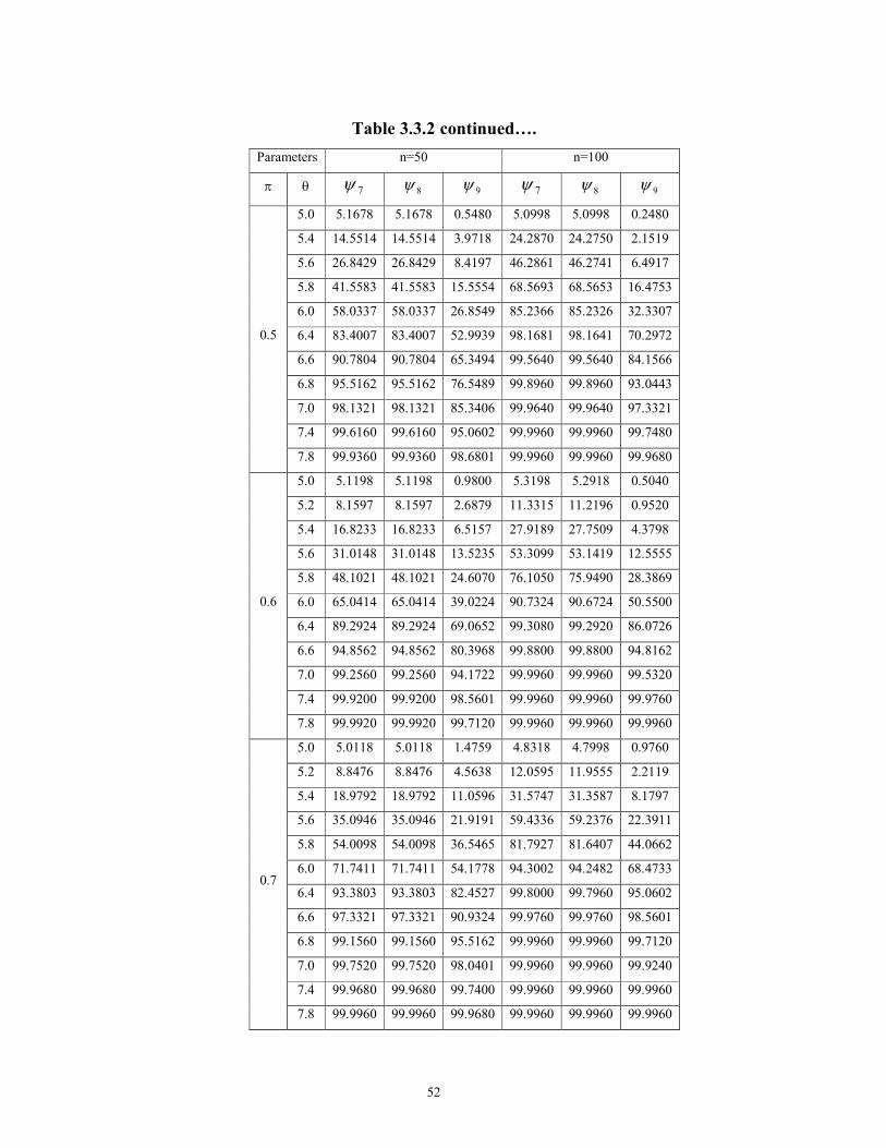
Table 3.3.2 continued….
Parameters n=50 n=100
π θ 7ψ 8ψ
9ψ 7ψ 8ψ
9ψ
5.0 5.1678 5.1678 0.5480 5.0998 5.0998 0.2480
5.4 14.5514 14.5514 3.9718 24.2870 24.2750 2.1519
5.6 26.8429 26.8429 8.4197 46.2861 46.2741 6.4917
5.8 41.5583 41.5583 15.5554 68.5693 68.5653 16.4753
6.0 58.0337 58.0337 26.8549 85.2366 85.2326 32.3307
6.4 83.4007 83.4007 52.9939 98.1681 98.1641 70.2972
6.6 90.7804 90.7804 65.3494 99.5640 99.5640 84.1566
6.8 95.5162 95.5162 76.5489 99.8960 99.8960 93.0443
7.0 98.1321 98.1321 85.3406 99.9640 99.9640 97.3321
7.4 99.6160 99.6160 95.0602 99.9960 99.9960 99.7480
0.5
7.8 99.9360 99.9360 98.6801 99.9960 99.9960 99.9680
5.0 5.1198 5.1198 0.9800 5.3198 5.2918 0.5040
5.2 8.1597 8.1597 2.6879 11.3315 11.2196 0.9520
5.4 16.8233 16.8233 6.5157 27.9189 27.7509 4.3798
5.6 31.0148 31.0148 13.5235 53.3099 53.1419 12.5555
5.8 48.1021 48.1021 24.6070 76.1050 75.9490 28.3869
6.0 65.0414 65.0414 39.0224 90.7324 90.6724 50.5500
6.4 89.2924 89.2924 69.0652 99.3080 99.2920 86.0726
6.6 94.8562 94.8562 80.3968 99.8800 99.8800 94.8162
7.0 99.2560 99.2560 94.1722 99.9960 99.9960 99.5320
7.4 99.9200 99.9200 98.5601 99.9960 99.9960 99.9760
0.6
7.8 99.9920 99.9920 99.7120 99.9960 99.9960 99.9960
5.0 5.0118 5.0118 1.4759 4.8318 4.7998 0.9760
5.2 8.8476 8.8476 4.5638 12.0595 11.9555 2.2119
5.4 18.9792 18.9792 11.0596 31.5747 31.3587 8.1797
5.6 35.0946 35.0946 21.9191 59.4336 59.2376 22.3911
5.8 54.0098 54.0098 36.5465 81.7927 81.6407 44.0662
6.0 71.7411 71.7411 54.1778 94.3002 94.2482 68.4733
6.4 93.3803 93.3803 82.4527 99.8000 99.7960 95.0602
6.6 97.3321 97.3321 90.9324 99.9760 99.9760 98.5601
6.8 99.1560 99.1560 95.5162 99.9960 99.9960 99.7120
7.0 99.7520 99.7520 98.0401 99.9960 99.9960 99.9240
7.4 99.9680 99.9680 99.7400 99.9960 99.9960 99.9960
0.7
7.8 99.9960 99.9960 99.9680 99.9960 99.9960 99.9960
53
From the simulation study reported in Tables (3.3.1) and (3.3.2), we observe
that
(i) The test based on full likelihood approach is better than the one
based on conditional likelihood approach when θ is small. However,
probability of Type–I error of the former test is more than that of later.
Therefore, we can consider the test based on conditional likelihood approach
as an alternative to the one based on full likelihood approach. The later test is
also easy for computations.
(ii) For large values of θ , both the tests are equally good.
Therefore, we recommend the use of conditional likelihood approach, when
θ is large. Conditional approach is proved to be an alternative to the full
likelihood approach for large values of θ . If θ is large, proportion of zeros
corresponding the Poisson distribution are relatively low. Hence these zeros
can be ignored while making inference about θ . However, for smaller values
of θ , such ignorance will have effect on inference of θ .
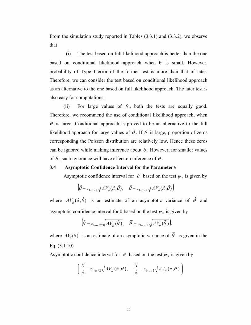
3.4 Asymptotic Confidence Interval for the Parameter θ
Asymptotic confidence interval for θ based on the test 7ψ is given by
( ))ˆ,ˆ(ˆ,)ˆ,ˆ(ˆˆ2/1ˆ2/1 θπθθπθθαθα AVzAVz −− +−
where )ˆ,ˆ(ˆ θπθ
AV is an estimate of an asymptotic variance of θ̂ and
asymptotic confidence interval for θ based on the test 8ψ is given by
( ))~(
~,)
~(
~~2/1~2/1 θθθθ θαθα AVzAVz −− +− .
where )~
(~ θAVθ
is an estimate of an asymptotic variance of θ~
as given in the
Eq. (3.1.10)
Asymptotic confidence interval for θ based on the test 9ψ is given by
+− −− ),ˆ(
ˆ,),ˆ(
ˆ2/12/1 θπ
πθπ
π θαθα AVzX
AVzX
54
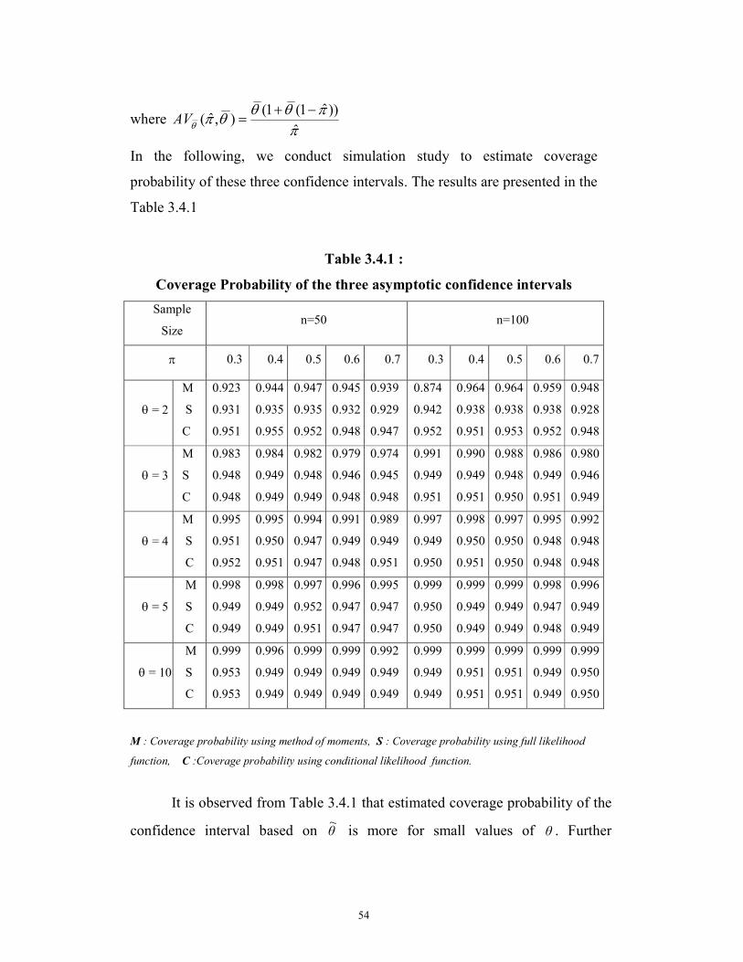
where ππθθ
θπθ ˆ
))ˆ1(1(),ˆ(
−+=AV
In the following, we conduct simulation study to estimate coverage
probability of these three confidence intervals. The results are presented in the
Table 3.4.1
Table 3.4.1 :
Coverage Probability of the three asymptotic confidence intervals
Sample
Size n=50 n=100
π 0.3 0.4 0.5 0.6 0.7 0.3 0.4 0.5 0.6 0.7
θ = 2
M
S
C
0.923
0.931
0.951
0.944
0.935
0.955
0.947
0.935
0.952
0.945
0.932
0.948
0.939
0.929
0.947
0.874
0.942
0.952
0.964
0.938
0.951
0.964
0.938
0.953
0.959
0.938
0.952
0.948
0.928
0.948
θ = 3
M
S
C
0.983
0.948
0.948
0.984
0.949
0.949
0.982
0.948
0.949
0.979
0.946
0.948
0.974
0.945
0.948
0.991
0.949
0.951
0.990
0.949
0.951
0.988
0.948
0.950
0.986
0.949
0.951
0.980
0.946
0.949
θ = 4
M
S
C
0.995
0.951
0.952
0.995
0.950
0.951
0.994
0.947
0.947
0.991
0.949
0.948
0.989
0.949
0.951
0.997
0.949
0.950
0.998
0.950
0.951
0.997
0.950
0.950
0.995
0.948
0.948
0.992
0.948
0.948
θ = 5
M
S
C
0.998
0.949
0.949
0.998
0.949
0.949
0.997
0.952
0.951
0.996
0.947
0.947
0.995
0.947
0.947
0.999
0.950
0.950
0.999
0.949
0.949
0.999
0.949
0.949
0.998
0.947
0.948
0.996
0.949
0.949
θ = 10
M
S
C
0.999
0.953
0.953
0.996
0.949
0.949
0.999
0.949
0.949
0.999
0.949
0.949
0.992
0.949
0.949
0.999
0.949
0.949
0.999
0.951
0.951
0.999
0.951
0.951
0.999
0.949
0.949
0.999
0.950
0.950
M : Coverage probability using method of moments, S : Coverage probability using full likelihood
function, C :Coverage probability using conditional likelihood function.
It is observed from Table 3.4.1 that estimated coverage probability of the
confidence interval based on θ~
is more for small values of θ . Further
55
investigation revealed that the same is at the cost of increase in the length of the
confidence interval. However, for large values of θ confidence interval based
on θ and θ~
perform equally good. However, the one based on method of
moment estimator does not perform satisfactorily. Investigations show that it
gives higher coverage due to increase in the length.
Example:
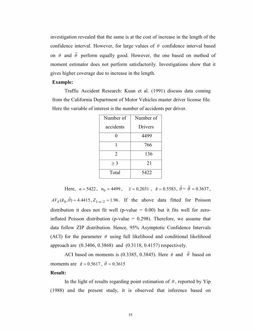
Traffic Accident Research: Kuan et al. (1991) discuss data coming
from the California Department of Motor Vehicles master driver license file.
Here the variable of interest is the number of accidents per driver.
Here, 5422=n , 44990 =n , 2031.0=x , 5583.0ˆ =π , θ̂ = 3637.0~=θ ,
4415.4)ˆ,ˆ( 0ˆ =θπAVπ , 96.12/1 =−αZ . If the above data fitted for Poisson
distribution it does not fit well (p-value = 0.00) but it fits well for zero-
inflated Poisson distribution (p-value = 0.298). Therefore, we assume that
data follow ZIP distribution. Hence, 95% Asymptotic Confidence Intervals
(ACI) for the parameter θ using full likelihood and conditional likelihood
approach are (0.3406, 0.3868) and (0.3118, 0.4157) respectively.
ACI based on moments is (0.3385, 0.3845). Here π̂ and θ based on
moments are 5617.0ˆ =π , 3615.0=θ
Result:
In the light of results regarding point estimation of θ , reported by Yip
(1988) and the present study, it is observed that inference based on
Number of
accidents
Number of
Drivers
0 4499
1 766
2 136
≥ 3 21
Total 5422
56
conditional likelihood approach is as good as the one based on full likelihood
approach. In the view of computational aspect, conditional likelihood
approach is recommended. This work is published in the journal Statistical
Methodology, 4(2007), 393-406.
In the following, we provide inference for zero-inflated truncated Poisson
distribution
3.5 Zero-Inflated Truncated Poisson distribution
Truncated samples from discrete distributions arise in numerous
situations where counts of zero are not observed. As an example, consider the
distribution of the number of children per family in developing nations, where
records are maintained only if there is at least a child in the family. The
number of childless families remains unknown. The resulting sample is thus
truncated with zero class missing. In continuous distribution, a sample of this
type would be described as singly left truncated. In other situations, sample
from discrete distributions might be censored on the right.
In this section, we consider zero-inflated truncated Poisson distribution
truncated at right at the support point ''t onwards, where ''t is known.
Moments, maximum likelihood estimators, Fisher information matrix for full
and conditional likelihood are provided. In the section 3.6, we provide three
tests for testing the parameter of the ZITPD.
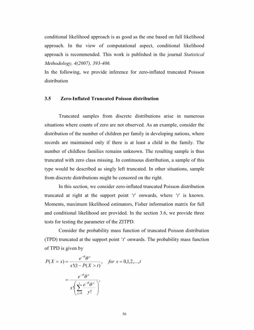
Consider the probability mass function of truncated Poisson distribution
(TPD) truncated at the support point ''t onwards. The probability mass function
of TPD is given by
txfortXPx
exXP
x
,...,2,1,0,)(1(!
)( =>−
==− θθ
,
!!
0
=
∑=
−
−
t
y
y
x
y
ex
e
θ
θθ
θ
57
,)(! θ
θAx
x
= where
= ∑
=
t
y
y
yA
0 !)(
θθ
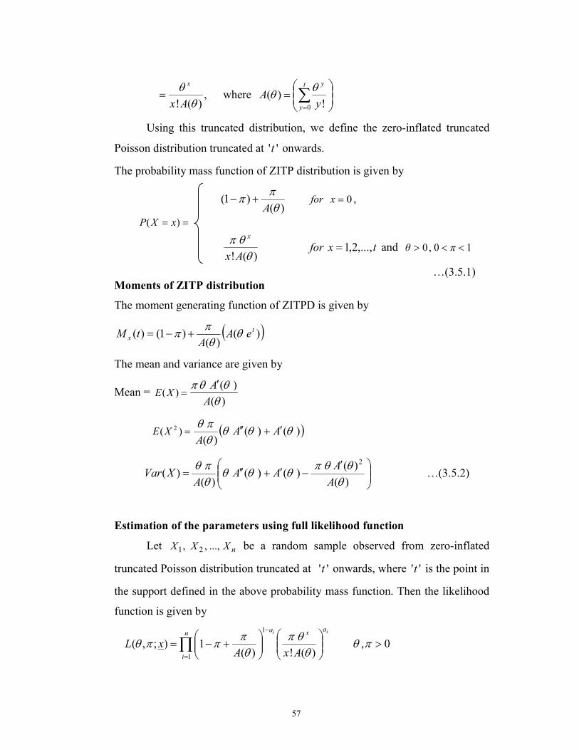
Using this truncated distribution, we define the zero-inflated truncated
Poisson distribution truncated at ''t onwards.
The probability mass function of ZITP distribution is given by
)(
)1(θπ
πA+− 0=xfor ,
== )( xXP
)(! θ
θπAx
x
txfor ,...,2,1= and 10,0 <<> πθ
…(3.5.1)
Moments of ZITP distribution
The moment generating function of ZITPD is given by
( ))()(
)1()( tx eA
AtM θ
θπ
π +−=
The mean and variance are given by
Mean = =)(XE)(
)(
θθθπ
A
A′
=)( 2XE ( ))()()(
θθθθπθ
AAA
′+′′
′−′+′′=
)(
)()()(
)()(
2
θθθπ
θθθθπθ
A
AAA
AXVar …(3.5.2)
Estimation of the parameters using full likelihood function
Let nXXX ...,,, 21 be a random sample observed from zero-inflated
truncated Poisson distribution truncated at ''t onwards, where ''t is the point in
the support defined in the above probability mass function. Then the likelihood
function is given by
0,)(!)(
1);,(
1
1
>
+−=
−
=∏ πθ
θθπ
θπ
ππθii a
xan
i AxAxL
58
The corresponding log likelihood function is given by
∑=
+
+−=
n
i
iaA
nxL1
0 log)(
1log);,(log πθπ
ππθ
∑ ∑∑= ==
−−+n
i
n
i
i
n
i
iiii Aaxaxa1 11
)(log!loglog θθ …(3.5.3)
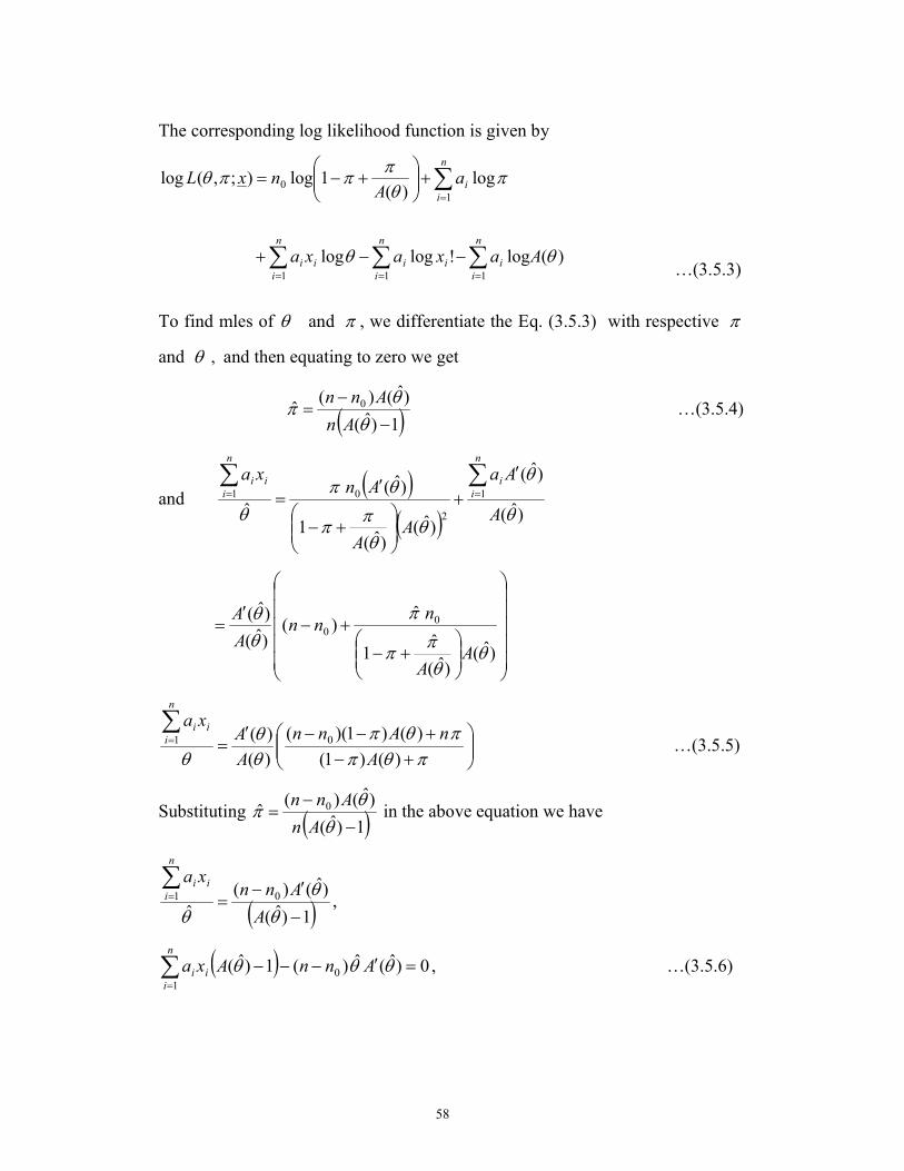
To find mles of θ and π , we differentiate the Eq. (3.5.3) with respective π
and θ , and then equating to zero we get
( )1)ˆ(
)ˆ()(ˆ 0
−
−=
θ
θπ
An
Ann …(3.5.4)
and ( )( ) )ˆ(
)ˆ(
)ˆ()ˆ(
1
)ˆ(
ˆ1
2
01
θ
θ
θθπ
π
θπ
θ A
Aa
AA
Anxa
n
i
i
n
i
ii′
+
+−
′=
∑∑==
+−
+−′
=
)ˆ()ˆ(
ˆ1
ˆ)(
)ˆ(
)ˆ( 00
θθπ
π
π
θθ
AA
nnn
A
A
+−
+−−′=
∑=
πθππθπ
θθ
θ )()1(
)()1)((
)(
)( 01
A
nAnn
A
Axa
n
i
ii
…(3.5.5)
Substituting ( )1)ˆ(
)ˆ()(ˆ 0
−
−=
θ
θπ
An
Ann in the above equation we have
( )1)ˆ(
)ˆ()(
ˆ01
−
′−=
∑=
θ
θ
θ A
Annxa
n
i
ii
,
( )∑=
=′−−−n
i
ii AnnAxa1
0 0)ˆ(ˆ)(1)ˆ( θθθ , …(3.5.6)
59
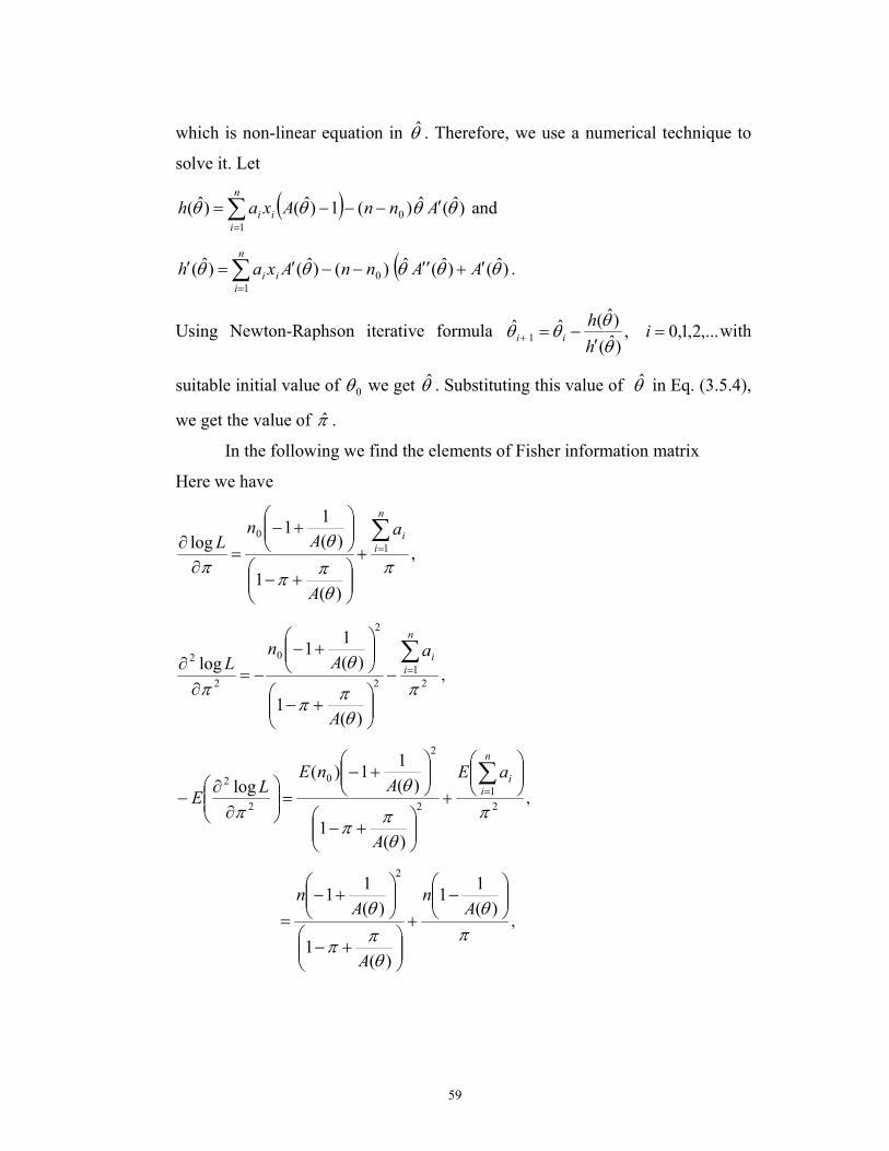
which is non-linear equation in θ̂ . Therefore, we use a numerical technique to
solve it. Let
( )∑=
′−−−=n
i
ii AnnAxah1
0 )ˆ(ˆ)(1)ˆ()ˆ( θθθθ and
( )ˆ()ˆ(ˆ)()ˆ()ˆ(1
0 θθθθθ AAnnAxahn
i
ii′+′′−−′=′ ∑
=
.
Using Newton-Raphson iterative formula ,...2,1,0,)ˆ(
)ˆ(ˆˆ1 =
′−=+ i
h
hii
θθ
θθ with
suitable initial value of 0θ we get θ̂ . Substituting this value of θ̂ in Eq. (3.5.4),
we get the value of π̂ .
In the following we find the elements of Fisher information matrix
Here we have
πθπ
π
θπ
∑=+
+−
+−
=∂∂
n
i
ia
A
An
L 1
0
)(1
)(
11
log,
2
1
2
2
0
2
2
)(1
)(
11
log
π
θπ
π
θπ
∑=−
+−
+−
−=∂
∂
n
i
ia
A
An
L,
2
1
2
2
0
2
2
)(1
)(
11)(
log
π
θπ
π
θπ
+
+−
+−
=
∂
∂−
∑=
n
i
iaE
A
AnE
LE ,
πθ
θπ
π
θ
−
+
+−
+−
=)(
11
)(1
)(
11
2
An
A
An
,
60
πθ
θπ
π
θπ
+−
−
+−
+−
=
∂
∂−
)(
11
)(1
)(
11
log
2
2
2 An
A
An
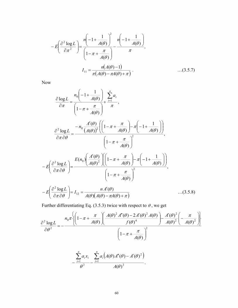
LE ,
( )( )πθπθπ
θ+−
−=
)()(
1)(11
AA
AnI . …(3.5.7)
Now
πθπ
π
θπ
∑=+
+−
+−
=∂∂
n
i
ia
A
An
L 1
0
)(1
)(
11
log,
( )
2
202
)(1
)(
11
)(1
)(
)(
log
+−
+−−
+−
′−
=∂∂
∂
θπ
π
θπ
θπ
πθθ
θπ
A
AAA
An
L,
2
202
)(1
)(
11
)(1
)(
)()(
log
+−
+−−
+−
′
=
∂∂∂
−
θπ
π
θπ
θπ
πθθ
θπ
A
AAA
AnE
LE ,
( )πθπθθθ
θπ +−
′==
∂∂∂
−)()()(
)(log12
2
AAA
AnI
LE …(3.5.8)
Further differentiating Eq. (3.5.3) twice with respect to θ , we get
2
22
2
4
22
0
2
2
)(1
)()(
)(
)(
)()(2)()(
)(1
log
+−
−
′−
′−′′
+−
−=∂
∂
θπ
π
θπ
θθ
θθθθθ
θπ
ππ
θ
A
AA
A
f
AAAA
An
L
( )2
1
2
2
1
)(
)()()(
θ
θθθ
θ A
AAAaxan
i
i
n
i
ii ∑∑==
′−′′−− .
61
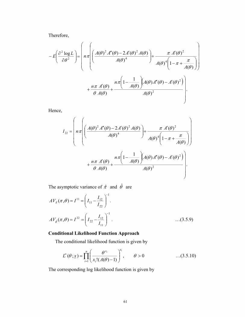
Therefore,
=
∂
∂−
2
2log
θL
E
+−
′+
′−′′
)(1)(
)(
)(
)()(2)()(
4
2
4
22
θπ
πθ
θπθ
θθθθπ
AA
A
A
AAAAn
( )
′−′′
−
+′
+2
2
)(
)()()()(
11
)(
)(
θ
θθθθ
π
θθθπ
A
AAAA
n
A
An.
Hence,
=22I
+−
′+
′−′′
)(1)(
)(
)(
)()(2)()(
4
2
4
22
θπ
πθ
θπθ
θθθθπ
AA
A
A
AAAAn
( )
′−′′
−
+′
+2
2
)(
)()()()(
11
)(
)(
θ
θθθθ
π
θθθπ
A
AAAA
n
A
An.
The asymptotic variance of π̂ and θ̂ are
1
22
1211
11ˆ ),(
−
−==
I
IIIAV θππ .
1
11
1222
22ˆ ),(
−
−==
I
IIIAV θπ
θ . …(3.5.9)
Conditional Likelihood Function Approach
The conditional likelihood function is given by
0,)1)((!
);(1
>
−=∏=
∗ θθθ
θn
i
a
i
x ii
AxxL …(3.5.10)
The corresponding log likelihood function is given by
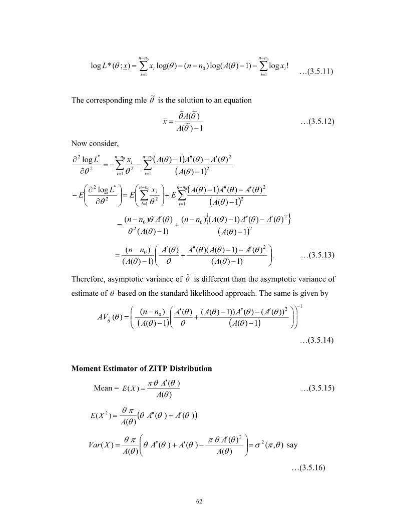
62
∑∑−
=
−
=
−−−−=00
1
0
1
!log)1)(log()()log();(*lognn
i
i
nn
i
i xAnnxxL θθθ …(3.5.11)
The corresponding mle θ~
is the solution to an equation
1)
~(
)~
(~
−=θθθ
A
Ax …(3.5.12)
Now consider,
( )( )∑∑
−
=
−
= −
′−′′−−−=
∂∂ 00
12
2
122
*2
1)(
)()(1)(log nn
i
nn
i
i
A
AAAxL
θθθθ
θθ
( )( )∑∑
−
=
−
= −
′−′′−+
=
∂
∂−
00
12
2
122
*2
1)(
)()(1)(log nn
i
nn
i
i
A
AAAE
xE
LE
θθθθ
θθ
{ }( )2
20
2
0
1)(
)()()1)(()(
)1)((
)()(
−
′−′′−−+
−
′−=
θ
θθθθθ
θθ
A
AAAnn
A
Ann
−
′−−′′+
′
−−
=)1)((
)()1)()(()(
)1)((
)( 20
θθθθ
θθ
θ A
AAAA
A
nn. …(3.5.13)
Therefore, asymptotic variance of θ~
is different than the asymptotic variance of
estimate of θ based on the standard likelihood approach. The same is given by
( ) ( )
12
0~
1)(
))(()())1)(()(
1)(
)()(
−
−
′−′′−+
′
−
−=
θθθθ
θθ
θθθ A
AAAA
A
nnAV
…(3.5.14)
Moment Estimator of ZITP Distribution
Mean = =)(XE)(
)(
θθθπ
A
A′ …(3.5.15)
=)(2
XE ( ))()()(
θθθθπθ
AAA
′+′′
),()(
)()()(
)()( 2
2
θπσθθθπ
θθθθπθ
=
′−′+′′=
A
AAA
AXVar say
…(3.5.16)
63
. )(
)(
θθθπ
A
Ax
′= …(3.5.17)
( ))()()(
1
2
θθθθπθ
AAAn
xn
i
i
′+′′=∑=
…(3.5.18)
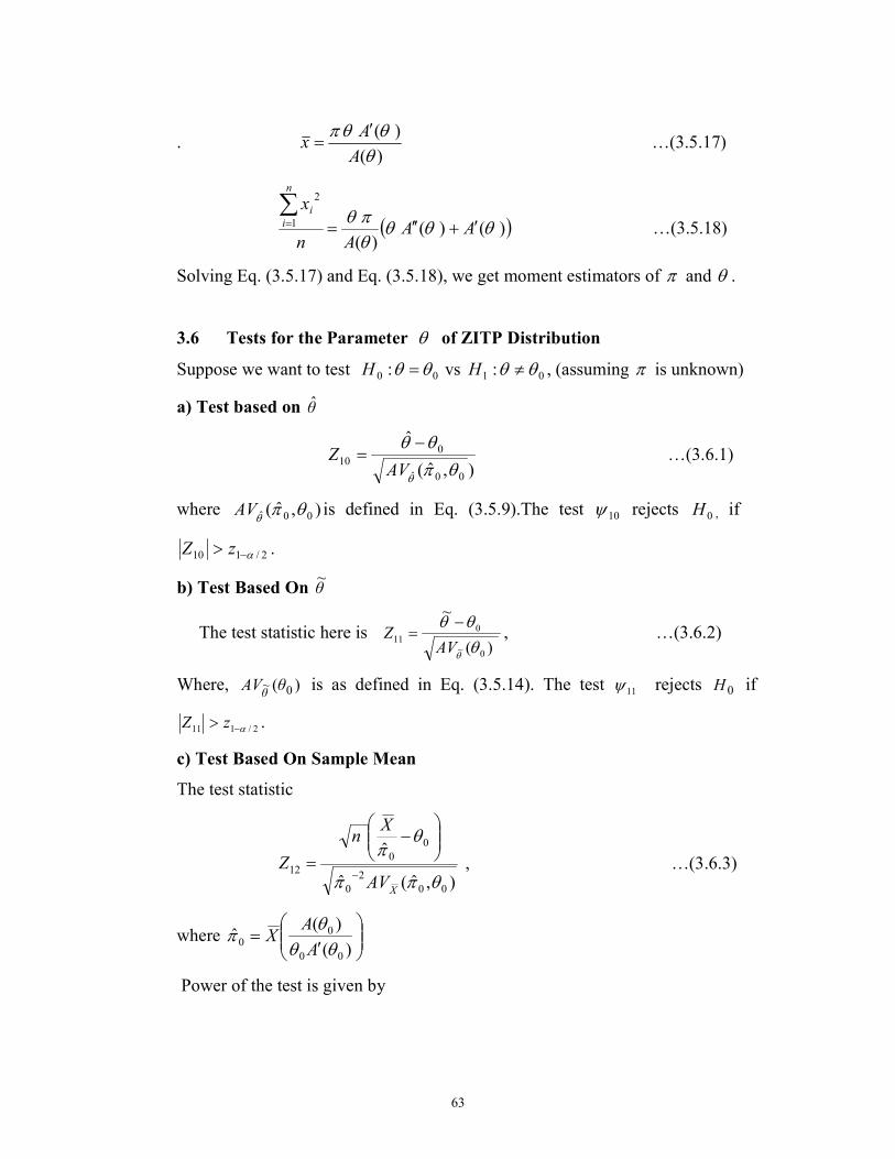
Solving Eq. (3.5.17) and Eq. (3.5.18), we get moment estimators of π and θ .
3.6 Tests for the Parameter θ of ZITP Distribution
Suppose we want to test 00 : θθ =H vs 01 : θθ ≠H , (assuming π is unknown)
a) Test based on θ̂
),ˆ(
ˆ
00ˆ
010
θπ
θθ
θAV
Z−
= …(3.6.1)
where ),ˆ( 00ˆ θπθ
AV is defined in Eq. (3.5.9).The test 10ψ rejects 0H , if
2/110 α−> zZ .
b) Test Based On θ~
The test statistic here is )(
~
0~
011
θ
θθ
θAVZ
−= , …(3.6.2)
Where, )( 0~ θAVθ
is as defined in Eq. (3.5.14). The test 11ψ rejects 0H if
2/111 α−> zZ .
c) Test Based On Sample Mean
The test statistic
),ˆ(ˆ
ˆ
00
2
0
0
0
12
θππ
θπ
XAV
Xn
Z−
−
= , …(3.6.3)
where
′
=)(
)(ˆ
00
00 θθ
θπ
A
AX
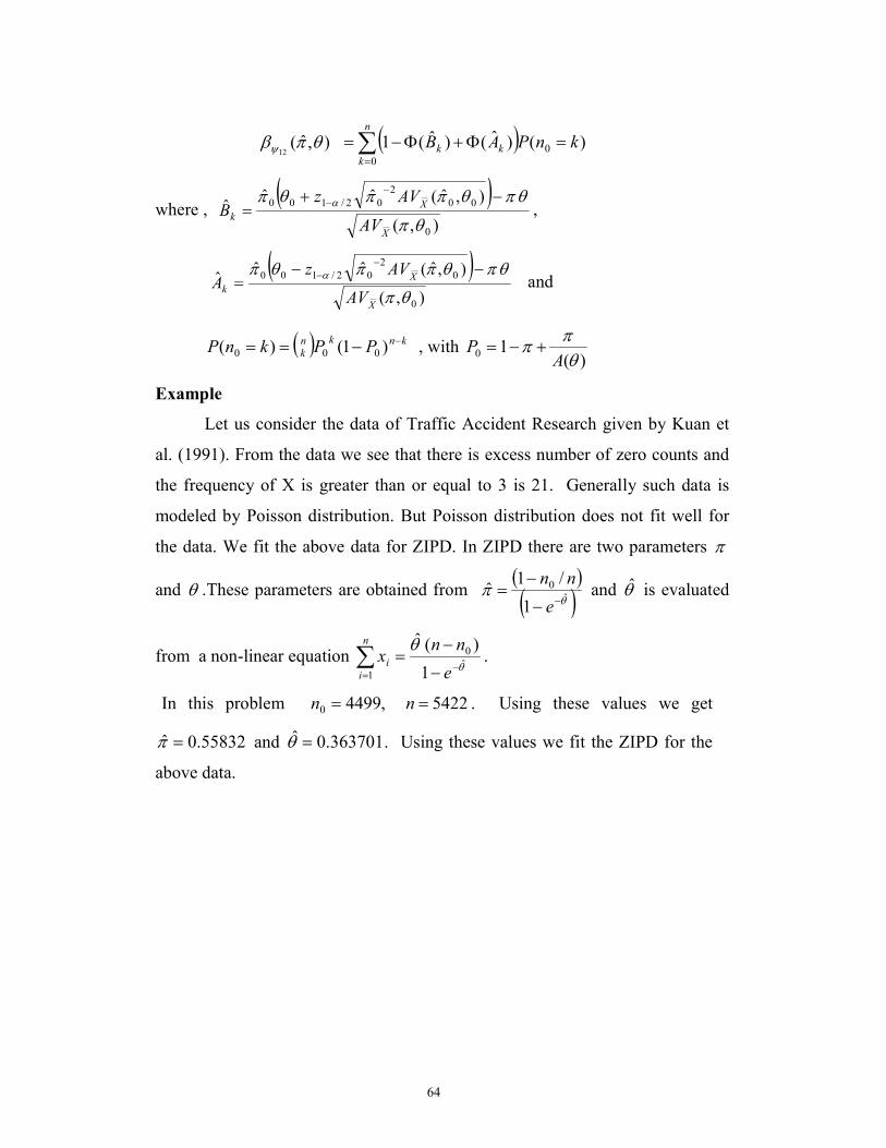
Power of the test is given by
64
),ˆ(12θπβψ ( )∑
=
=Φ+Φ−=n
k
kk knPAB0
0 )()ˆ()ˆ(1
where , ( )
),(
),ˆ(ˆˆˆ
0
00
2
02/100
θπ
θπθππθπ α
X
X
kAV
AVzB
−+=
−−
,
( )
),(
),ˆ(ˆˆˆ
0
0
2
02/100
θπ
θπθππθπ α
X
X
kAV
AVzA
−−=
−−
and
( ) knknk PPknP −−== )1()( 000 , with
)(10 θ
ππ
AP +−=
Example
Let us consider the data of Traffic Accident Research given by Kuan et
al. (1991). From the data we see that there is excess number of zero counts and
the frequency of X is greater than or equal to 3 is 21. Generally such data is
modeled by Poisson distribution. But Poisson distribution does not fit well for
the data. We fit the above data for ZIPD. In ZIPD there are two parameters π
and θ .These parameters are obtained from ( )( )θπ
ˆ
0
1
/1ˆ
−−
−=
e
nn and θ̂ is evaluated
from a non-linear equation θ
θˆ
0
1 1
)(ˆ
−= −
−=∑
e
nnx
n
i
i .
In this problem 5422,44990 == nn . Using these values we get
55832.0ˆ =π and 363701.0ˆ =θ . Using these values we fit the ZIPD for the
above data.
65
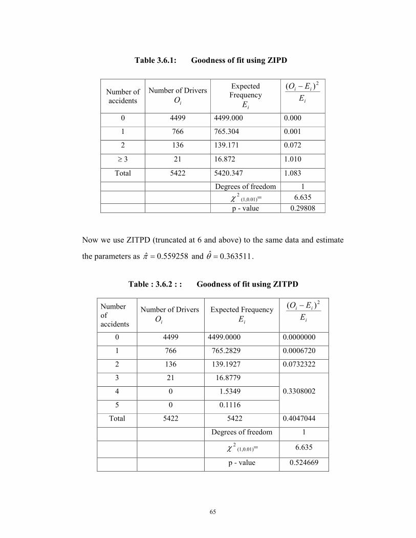
Table 3.6.1: Goodness of fit using ZIPD
Now we use ZITPD (truncated at 6 and above) to the same data and estimate
the parameters as 559258.0ˆ =π and 363511.0ˆ =θ .
Table : 3.6.2 : : Goodness of fit using ZITPD
Number of
accidents
Number of Drivers
iO
Expected
Frequency
iE i
ii
E
EO 2)( −
0 4499 4499.000 0.000
1 766 765.304 0.001
2 136 139.171 0.072
≥ 3 21 16.872 1.010
Total 5422 5420.347 1.083
Degrees of freedom 1
2χ (1,0.01)= 6.635
p - value 0.29808
Number
of
accidents
Number of Drivers
iO
Expected Frequency
iE i
ii
E
EO 2)( −
0 4499 4499.0000 0.0000000
1 766 765.2829 0.0006720
2 136 139.1927 0.0732322
3 21 16.8779
4 0 1.5349
5 0 0.1116
0.3308002
Total 5422 5422 0.4047044
Degrees of freedom 1
2χ (1,0.01)= 6.635
p - value 0.524669
66
From the Table 3.6.1, we observed that calculated chi square value
(1.083) is less than the table value of 2χ (1,0.01) = 6.635. Therefore, we accept
the hypotheses and conclude that ZIPD fits well. The P value is 0.29808.
From Table : 3.6.2 we can observe that calculated chi square value
(0.4047044) is less than the table value of 2χ (1,0.01) = 6.635 and the p-value is
0.524669. As p-value for ZIPD is less than the p-value for ZITPD, we prefer
ZITPD to model the data.
The ZIP distribution has been shown to be useful for modeling
outcomes of manufacturing process producing numerous defect-free products.
When there are several types of defects, the multivariate ZIP model can be
useful to detect specific process equipment problems and to reduce multiple
types of defects simultaneously. In the next chapter, we introduce Bivariate
ZIPSD and Bivariate ZIPD and discuss the inference related to the parameters
involved in the model.