on the risk capital framework of financial institutions on the risk capital framework of financial...

83

On the Risk Capital Framework of Financial Institutions

Tatsuya Ishikawa, Yasuhiro Yamai, and Akira Ieda

Tatsuya Ishikawa: Research Division I, Institute for Monetary and Economic Studies,Bank of Japan (currently Risk Management Department, UFJ Holdings, Inc.)(E-mail: [email protected])

Yasuhiro Yamai: Research Division I, Institute for Monetary and Economic Studies (currently Bank Examination and Surveillance Department), Bank of Japan(E-mail: [email protected])

Akira Ieda: Research Division I, Institute for Monetary and Economic Studies, Bank ofJapan (E-mail: [email protected])

The views expressed here are those of the authors and do not necessarily reflect those of the Bank of Japan, the Institute for Monetary and Economic Studies, the BankExamination and Surveillance Department, or UFJ Holdings, Inc.

MONETARY AND ECONOMIC STUDIES/OCTOBER 2003

In this paper, we consider the risk capital framework adopted byfinancial institutions. Specifically, we review the recent literature on this issue, and clarify the economic assumptions behind thisframework. Based on these observations, we then develop a simplemodel for analyzing the economic implications of this framework.

The main implications are as follows. First, risk capital allocationsare theoretically unnecessary without deadweight costs for raising capital, which are not usually assumed in the business practices of financial institutions. Second, the risk-adjusted rate of return isredundant as it provides no additional information beyond the netpresent value. Third, risk capital allocation is intrinsically difficultbecause it is hard to incorporate the correlations among asset returns.

Keywords: Risk capital; Risk management; Capital structure;Capital budgeting; Risk-adjusted rate of return; Capitalallocation; Deadweight cost

JEL Classification: G20

MONETARY AND ECONOMIC STUDIES/OCTOBER 2003

DO NOT REPRINT OR REPRODUCE WITHOUT PERMISSION.

I. Introduction

In recent years, an increasing number of financial institutions have adopted risk capital frameworks.1 Under these frameworks, banks determine the amount of capitalneeded to cover their risk, and measure their risk-adjusted performance. According toZaik et al. (1996), James (1996), and Matten (2000), the elements of the risk capitalframeworks adopted by financial institutions are as follows.

(1) Holding sufficient capital to cover riskFinancial institutions hold a sufficient amount of capital to cover the risk oftheir business activities (this capital is called “risk capital”). They determinethe amount of risk capital as the unexpected losses of their operations. Theymeasure the unexpected losses using value-at-risk and other risk measures.

(2) Allocating risk capital to each operating divisionFinancial institutions allocate risk capital to individual lines of businessaccording to their respective risks.

(3) Evaluating profitability based on risk-adjusted rates of returnFinancial institutions evaluate the performance of individual lines of businessusing their respective “risk-adjusted rates of return” (profit divided by allocatedrisk capital).

In this paper, we call this framework the “standard framework” of risk capital andconsider its economic implications. We consider this framework as the representativeexample of risk capital frameworks, since it is both typical and common to the business practices of financial institutions.2

This standard framework assumes that financial institutions are risk-averse decision-makers and make investment decisions based on risk-return trade-offs.However, finance theory does not assume, a priori, that financial institutions are risk-averse decision-makers. Rather, finance theory says that a firm is primarily anexus of contracts, and that a firm is risk-neutral in a perfect market (Modigliani andMiller [1958]). Therefore, to justify the risk capital framework from the theoreticalviewpoint, we must establish the reason why financial institutions are risk-averse.

Since the 1990s, a number of research papers have addressed this issue3 from theviewpoint of finance theory. They establish how and why financial institutions are risk-averse and propose risk capital frameworks that are well aligned with theireconomic analyses.

In this paper, we consider the risk capital framework generally adopted at financialinstitutions. Specifically, we review the recent literature and clarify the economicassumptions behind this framework. Based on these observations, we then develop asimple model for analyzing the economic implications of this framework.

84 MONETARY AND ECONOMIC STUDIES/OCTOBER 2003

1. The “risk capital framework” characterized here is also called “integrated risk management” or the “risk-adjustedreturn on capital (RAROC) system.”

2. There are several variations to this framework. See Zaik et al. (1996), James (1996), and Matten (2000).3. Froot and Stein (1998) examine the capital of financial institutions, explicitly incorporating the concavity of the

payoff under the existence of economic friction. Merton and Perold (1993) argue that risk capital is viewed asinsurance purchased as required against bankruptcy. Crouhy et al. (1999) define risk capital as the risk-free assetsrequired to restrain the probability of bankruptcy to within a certain level, and primarily address capital budgetingdecision-making problems.

The main findings are as follows.• The allocation of risk capital is theoretically unnecessary when we do not

assume the deadweight costs of raising capital. As the deadweight costs of raisingcapital are not usually assumed in the business practices of financial institutions,the allocation of risk capital seems unnecessary for practical use.

• The risk-adjusted rate of return in the standard framework is equivalent to thenet present value (NPV). The risk-adjusted rate of return is inferior to the NPV,since the former requires the calculation of risk capital (i.e., value-at-risk) whilethe latter does not.

• The allocation of risk capital is intrinsically difficult, as we must consider the correlations among asset returns.

In the first half of this paper (through Section III), we describe the theories presented in the prior research on risk capital. In Section II, we consider a firm’sfinancing decision-making in a perfect market. In a perfect market, the Modigliani-Miller proposition (hereafter the “MM proposition”) holds and risk capital plays norole in financing decision-making. In Section III, we introduce economic frictionsuch as bankruptcy costs and information asymmetry. With economic friction, a firmbecomes risk-averse and risk capital plays some roles. We also note that economicfriction is more serious for financial institutions than for nonfinancial firms. Thus,risk capital plays greater roles at financial institutions than at other firms.

In the second half of this paper (from Section IV onward), we develop a simple model for analyzing the standard framework. From this model, we derive the economic implications of the risk capital framework in Section IV, and then consider the difficulty of risk capital allocation in Section V. Section VI presents the conclusions.

II. Financing Decisions in a Perfect Market

In this section, we describe a firm’s4 capital structure, risk management, and capitalbudgeting under a perfect market.5 This description prepares for the discussions ofrisk capital in subsequent sections.

A. The MM PropositionThe MM proposition, stated in Modigliani and Miller (1958), is the most importantfactor in considering a firm’s capital structure in a perfect market. Based on the MMproposition, Fama (1978) demonstrates that in a perfect market that satisfies the following conditions, how firms raise funds has no influence on their value.

(1) Frictionless market (there are no transaction costs or taxes, and all assets areperfectly divisible and marketable).

85


4. We make no distinctions between financial institutions and nonfinancial firms in this section, as we only considerthe decision-making in a perfect market.

5. See Brealey and Myers (2000), McKinsey & Company Inc. et al. (2000), and Damodaran (1999) for firms’financing decision-making in a perfect market.

(2) Information efficiency (all investors, firms, and firms’ managers have the same information, and hold homogeneous expectations regarding how thisinformation will affect market prices).

(3) Given investment decisions (the investment decisions are given conditions,and are completely independent from the decisions on raising new externalfunds).

(4) Equal access (all market participants can issue securities under the same terms).The essence of the MM proposition is that a firm’s capital structure does not

matter, because investors can arrange their own desired payoffs by adjusting theirportfolios by themselves.

The MM proposition also says that a firm’s risk management does not matter in aperfect market. A firm has no need to hedge the tradable risks it is exposed to,because the investors who invest in its stocks or bonds can hedge the firm’s risks bytrading those risks by themselves. So, in a perfect market where the MM propositionholds, one cannot assume, a priori, that a firm is risk-averse.

In the following subsections, we explicate the firm’s decision-making in a perfectmarket, where the MM proposition holds, using the asset pricing model.

B. Asset PricingTo examine how risk management and capital structure affect the firm’s value, we need to calculate the present value of the firm’s future payoff (hereafter “the firm’s value”). In this paper, we adopt the Capital Asset Pricing Model (CAPM6 ) todetermine the present value of the future uncertain payoff.

We adopt a two-period model (period 0 and period 1). Under CAPM, equation(1) shows the relationship between the rate of return ri for a given asset i and the rateof return for the market portfolio (the market return).7

E [ri] = rf + �i(E [rM] − rf ), (1)

where8 �i = cov(ri , rM)/var(rM), rM is market return, rf is the risk-free rate, and �i is aconstant for each asset.

Here, the random variable Xi indicates the asset’s payoff at period 1, and P (Xi)indicates the asset’s present value at period 0. By definition of ri,

E [Xi] 1 + E [ri] = ——–. (2)P (Xi)

Substituting equation (2) into equation (1), and using � ≡ (E [rM] − rf )/var(rM )which is not dependent on the characteristics of each asset, the value of P (Xi) is thendetermined as shown in equation (3).


6. The argument in this paper could also be developed using a wider class of pricing models that can be nested in thestochastic discount factor model. See Cochrane (2001) for the details of the stochastic discount factor.

7. E [•] represents the expectation operator with the given information at period 0.8. cov(X, Y ) expresses the covariance of the random variables X and Y, and var(X ) expresses the variance of the

random variable X.

E [Xi ] − � cov(Xi , rM) P(Xi ) = ————————–. (3)1 + rf

C. Capital Budgeting, Capital Structure, and Risk Management in a Perfect Market

Next, we explain a firm’s financing decision-making (capital budgeting, capital structure, and risk management) in a perfect market, where the MM propositionholds. In this paper, capital budgeting, capital structure, and risk management decision-making are defined as follows.

(1) Capital budgetingTo decide how much to invest in an investment opportunity.

(2) Capital structureTo select how the investment is financed. For simplicity, we assume that a firmcan finance only with common stocks and straight bonds.

(3) Risk managementTo decide whether or not to hedge the tradable risks that a firm is exposed to.

In this paper, those three decisions are collectively referred to as the firm’s “financing decision-making.”

The firm’s NPV is expressed by equation (4), where P (X ) represents the firm’spresent value and I represents the amount of capital.

NPV = P (X ) − I . (4)

One of the most important characteristics of a firm’s financing decision-making ina perfect market is “value additivity.”9 The concept of value additivity is as follows.Suppose there are two investment opportunities A and B with payoffs XA and XB,respectively, and their present values are P (XA) and P (XB). Value additivity holdswhen the sum of these present values is the same as the present value of the twoinvestment opportunities taken together, that is, where P (XA + XB) = P (XA) + P (XB).From equation (3), value additivity holds when the following holds.

E [XA + XB] − � cov(XA + XB, rM) P (XA + XB) = ————————————– 1 + rf

E [XA] − � cov(XA, rM) E [XB] − � cov(XB, rM) = ————————– + ————————– 1 + rf 1 + rf

= P (XA) + P (XB). (5)

Value additivity results from the linearity of the present value P (X ) to the payoff X .

87


9. See Brealey and Myers (2000) for a detailed introduction to value additivity.

Additionally, because IA+B = IA + IB, the NPV is also value additive as shown inequation (6).

NPVA + NPVB = {P (XA) − IA } + {P (XB) − IB}

= {P (XA) + P (XB)} − {IA + IB}

= P (XA + XB) − {IA + IB}

= NPVA+B. (6)

This value additivity has the following important implications for the firm’sfinancing decision-making.

(1) Capital budgetingThe capital budgeting decisions on multiple investment opportunities areindependent of each other when value additivity holds. As is clear from equation (6),10 the NPV of one investment opportunity is independent of theNPV of another investment opportunity. For example, suppose that a firm hastwo operating divisions, and they both implement capital budgeting. If eachdivision independently maximizes its NPV without any consideration for theother, the NPV of the firm will also be maximized.

(2) Capital structureValue additivity is equivalent to the MM proposition that capital structuredoes not matter. This can be shown as follows.11 Let a random variable Xindicate a firm’s payoff at period 1. When the firm’s only means of fund-raising is the issuance of stocks, the firm’s value becomes P1 = P (X ). Next,consider the firm’s value when the firm can raise funds by issuing stocksand/or bonds. When the stock and bond payoffs at period 1 are S and D,respectively, the firm’s present value P2 is the sum of those of the stocks andbonds, so P2 = P (S ) + P (D). As the firm’s overall payoff at period 1 can bedivided into those of stocks and bonds, X = S + D. Because of the value additivity, it can then be demonstrated that P1 = P2, as in equation (7).

P1 = P (X ) = P (S + D) = P (S ) + P (D) = P2. (7)

(3) Risk managementValue additivity is equivalent to the irrelevance of risk management.12 This can be shown by the following example. Let a random variable X indicate afirm’s payoff at period 1. Suppose that the variability of the firm’s payoff X canall be hedged by market trading, specifically by a forward contract of the


10. Rather than utilizing equation (3), practitioners commonly calculate the present value using a modified version of equation (2): P (Xi ) = E (Xi )/(1 + ri ). In this case, although it is necessary to calculate the value of ri (or �i ) for each investment opportunity, a single value is often adopted for an entire firm. If the individual investmentopportunity’s � were always equal to (or nearly equal to) the firm’s �, this would not present many problems. Sincethis is not the case, the use of the P (Xi ) = E (Xi )/(1 + ri ) equation is generally inappropriate, as detailed below.

11. See Ross (1978) for this proof of the MM proposition.12. See Culp (2001) for a more detailed explanation.

payoff ’s underlying assets. In a perfect market, the NPV of the forward contract (F – X , where the forward delivery price is F ) is zero.13 In otherwords, equation (3) can be restated as follows.

E [F − X ] − � cov(F − X , rM) 0 = ————————————. (8)

1 + rf

Thus, the forward delivery price F can be expressed as follows.14

F = E [X ] − � cov(X , rM). (9)

Here, after the risk on the payoff X is hedged and the payoff becomes the forward delivery price F, the firm’s value after the hedge P ′1 becomes identicalto the firm’s value before the hedge P (X ).

E [F ] − � cov(F, rM) F E [X ] − � cov(X , rM)P ′1 = P (F ) = ———————— = ——– = ————————

1 + rf 1 + rf 1 + rf

= P (X ). (10)

Therefore, because of the value additivity, the firm’s hedge operation does notchange its value. Thus, risk management is irrelevant when value additivityholds.

III. Financing Decisions in a Real Market

A. Existence of Economic FrictionIn the previous section, we assumed a perfect market. In a perfect market, value addi-tivity holds and capital structure and risk management are irrelevant. As shown in theprevious section, value additivity is based on the linear relationship between the NPVand the payoff. Thus, the irrelevance of capital structure and risk managementdepends on this linear relationship.

In the real world, the firm’s NPV may not be a linear function of the payoff. This is usually due to the existence of “economic friction”15 such as bankruptcy costsand progressive corporate tax rates. This friction places costs on the firm that have aconvex function with the payoff.

89


13. In a perfect market, the NPV of market trading is always zero. This can be explained as follows. Assume a giventrading opportunity with a positive NPV in a perfect market. Because all the participants can freely engage in trading, they would all take advantage of this trading opportunity. This would result in a surplus demand for this trading opportunity, so the market price would then move downward, reducing the NPV. This market priceadjustment would continue until the NPV declines to zero, and reach equilibrium when the NPV equals zero. In a perfect market, this price adjustment would be done instantaneously. Thus, market trading with a positiveNPV cannot exist in a perfect market.

14. From equation (3), E [X ] = (1 + rf )P (X ) + � cov(X , rM), so F = (1 + rf )P (X ). This is the forward delivery pricederived from the non-arbitrage conditions whereby there are no risk-free profits.

15. Although the agency problem is also an important reason for the imperfection of financial markets, it is notaddressed in this paper. See Barnea et al. (1985) for the details of the agency problem.

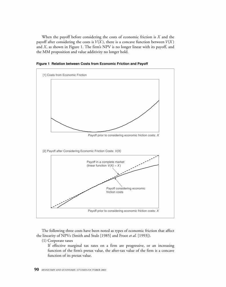
When the payoff before considering the costs of economic friction is X and thepayoff after considering the costs is V (X ), there is a concave function between V (X )and X , as shown in Figure 1. The firm’s NPV is no longer linear with its payoff, andthe MM proposition and value additivity no longer hold.


Figure 1 Relation between Costs from Economic Friction and Payoff

Payoff prior to considering economic friction costs: X

[1] Costs from Economic Friction

Payoff prior to considering economic friction costs: X

[2] Payoff after Considering Economic Friction Costs: V(X)

Payoff in a complete market (linear function V(X) = X )

Payoff considering economic friction costs

The following three costs have been noted as types of economic friction that affectthe linearity of NPVs (Smith and Stulz [1985] and Froot et al. [1993]).

(1) Corporate taxes If effective marginal tax rates on a firm are progressive, or an increasing function of the firm’s pretax value, the after-tax value of the firm is a concavefunction of its pretax value.

(2) Bankruptcy costsA firm must pay bankruptcy costs,16 such as legal and administrative costs,when the firm’s value is below its debt level. Thus, the bankruptcy costs arehigh when the firm’s value is low. This results in a concavity between the payoff before the bankruptcy costs and the payoff after the bankruptcy costs.

(3) Higher cost of raising external capitalDue to agency and information problems, new external capital is more expensive than internal capital. Froot et al. (1993) demonstrate that the payofffunction becomes increasingly convex from raising external capital. They statethat declines in the firm’s payoff deplete internal reserves, and then lead to ahigher level of dependence on external capital. When external capital is moreexpensive than internal capital, this growing dependence on external capitalimposes a higher cost on the firm.

B. Payoff Concavity and Value Non-AdditivityWe explained how the costs of economic friction result in a concave functionbetween the payoffs before the costs are considered and the payoffs after the costs are considered.

We now demonstrate that the firm’s value is not value additive when the payofffunction is concave. Suppose the firm’s payoff before considering the costs of economic friction is X and the payoff after considering the costs is V. Also suppose Vis a concave function of X , as follows.

V = V (X ), where V ′(•) > 0, V ″(•) < 0. (11)

Using equation (3), the firm’s value can now be expressed as equation (12).

E [V (X )] − � cov(V (X ), rM)P (V (X )) = ———————————. (12)

1 + rf

Since V (•) is a concave function, as shown in equation (13), there is no valueadditivity.

E [V (XA + XB)] − � cov(V (XA + XB), rM) P (V (XA + XB)) = ———————————————

1 + rf

E [V (XA)] − � cov(V (XA), rM) E [V (XB)] − � cov(V (XB), rM)≠ ——————————— + ——————————— 1 + rf 1 + rf

= P (V (XA)) + P (V (XB)). (13)

91


16. There are two types of bankruptcy costs: direct and indirect. The direct costs of bankruptcy are the costs of processing bankruptcy procedures such as legal and administrative costs. The indirect costs of bankruptcy includethe costs of deterioration of the firm’s business from the bankruptcy procedure. See Brealey and Myers (2000) fordetails of bankruptcy costs.

Because there is no value additivity, the conclusions reached for the firm’s financing decision-making in a perfect market no longer hold. In other words, thefirm’s financing decision-making in a real market is far more complex compared withthat in a perfect market.

C. Economic Friction at Financial InstitutionsThus far, we have made no distinction between financial institutions and non-financial firms. However, economic friction has a greater influence on the former than the latter. Merton and Perold (1993) note that bankruptcy costs and informationcosts are more remarkable at financial institutions than at nonfinancial firms.

(1) Bankruptcy costsThe major customers of financial institutions can be major liability holders;for example, policyholders, depositors, and swap counterparties are all liability holders as well as customers. When the bankruptcy risk at a financialinstitution rises, customers typically move to other financial institutions. This exodus of customers imposes another indirect cost on the strugglingfinancial institution, because it loses the profits that would otherwise havebeen derived.

An exodus of customers may also occur at nonfinancial firms, but theimpact is far greater at financial institutions because their customers, especiallythose who are outside of the deposit insurance safety net, are extremely sensitiveto bankruptcy risk. Thus, the bankruptcy costs at financial institutions17 are fargreater than those at nonfinancial firms.

(2) Information costsIn general, financial institutions do not disclose their assets or activities ingreat detail, and thus their business appears opaque to customers andinvestors.18 That is, the detailed asset holdings and business activities of thefirm are not publicly disclosed (or, if disclosed, only with a considerable lag intime). Furthermore, principal financial firms typically have relatively liquidbalance sheets that, in the course of just weeks, can and often do undergo substantial changes in size and risk. The information asymmetry between themanagement of financial institutions and outsiders leads to the problem ofhigher costs of raising external capital (Myers and Majluf [1984]). As a result,the problem of higher costs of raising external capital is more serious at financial institutions than at nonfinancial firms.

Froot and Stein (1998) develop a framework for analyzing the capital allocationand capital structure decisions of financial institutions incorporating economic friction. In their framework, they propose a two-factor model that can be used forcapital budgeting problems at financial institutions. With the model, they clarify theroles of economic friction on the financing decision-making of financial institutions.


17. See Merton (1997) for a discussion of the scale of bankruptcy costs at financial institutions.18. The “opaqueness” of financial institutions is first noted in Ross (1989).

However, the framework of Froot and Stein (1998) is not widely adopted in thepractices of financial institutions. As they note, their framework requires calculationof the concavity of the payoff function (V (•) in equation [11]), which is hard to measure in practice. Instead, financial institutions adopt risk capital frameworks,which are not consistent with the framework of Froot and Stein (1998).

IV. Standard Framework

In this section, we analyze the risk capital frameworks adopted by financial institutions. As noted in Section I, we use the “standard framework” as a generalizedexample of the risk capital frameworks. The elements of the standard framework areas follows.

(1) Holding sufficient capital to cover riskFinancial institutions hold a sufficient amount of capital to cover the risk of their business activities (this capital is called “risk capital”). They determine the amount of risk capital as the unexpected losses of their operations. They measure the unexpected losses using value-at-risk and otherrisk measures.

(2) Allocating risk capital to each operating divisionFinancial institutions allocate risk capital to individual lines of businessaccording to their respective risks.

(3) Evaluating profitability based on risk-adjusted rates of returnFinancial institutions evaluate the performance of individual lines of businessusing their respective “risk-adjusted rates of return” (profit divided by allocatedrisk capital).

In this section, we first demonstrate how the standard framework can be developed into a model (hereafter, the “standard model”) by positing assumptionsthat simplify the firm’s payoff. We then examine the economic implications of thestandard framework of risk capital adopted by financial institutions.

Also, we limit our considerations of the standard framework in this section to elements (1) “holding sufficient capital to cover risk” and (3) “evaluating profitabilitybased on risk-adjusted rates of return.” We proceed with considerations of element(2) “allocating risk capital to each operating division” in the subsequent section.

A. Basic Concept of the Standard FrameworkThe basic concept of the standard framework is “holding sufficient capital to coverrisk.” More precisely, the risk is quantified using value-at-risk or other risk measuresand capital equal to or greater than the calculated risk is held as a buffer against it.

B. Standard ModelWe develop the standard model based on the setup presented by Froot and Stein(1998), as follows. The model has two time periods, period 0 and period 1. Weassume that a financial institution invests in an investment opportunity that will generate a per unit payoff of X at period 1. At period 0, X is a random variable with a

93


mean of �. Note that we do not have to assume that X obeys a normal distribution.We also assume that this investment opportunity is available for an infinite numberof units and that the investment can be implemented without cost.

Meanwhile, this financial institution raises an amount of capital K at period 0,and invests the proceeds in a risk-free asset. The following discussions throughSection IV.E all assume that this amount of capital K is exogenously given.

The financial institution makes an investment of � units in the investmentopportunity. Now, we introduce the standard framework whereby the institutionretains sufficient capital to cover the risk. In this paper, we assume the linear homogeneity presented in equation (14) for the amount of risk �(•).

�(�X ) = ��(X ). (14)

The financing decision-making of the institution takes place under the restrictionsexpressed by equation (15).

�(�X ) ≤ K . (15)

Equation (15) may be viewed as a function expressing the financial institution’s“behavioral principle” under the standard framework of risk capital whereby the risk may not exceed the risk capital. We assume that the payoff for this financial institution is as expressed in equations (16) and (17).

V (w) = w, when �(�X ) ≤ K . (16)

w = �X + (1 + rf )K . (17)

Equation (16) says that economic friction is nonexistent as long as the capital covers the risk of the financial institution. This is the basic principle of the standard framework.19 Given the linear homogeneity, equation (15) can be rewritten as follows.

K� ≤ ——–. (18)�(X )

The institution’s NPV can now be expressed as follows based on equations (16)and (17).


19. Some may argue that the standard framework of risk capital assumes a convex function for a firm’s value. If weassume a convex function, however, the firm’s financing decision-making would be the same as that in Froot andStein (1998), which is not widely adopted by financial institutions.

E [w] − � cov(w, rM) NPV = P (V (w)) − K = P (w) − K = ———————— − K

1 + rf

E [�X + (1 + rf )K ] − � cov(�X + (1 + rf )K , rM) = ——————————————————— − K1 + rf

�E [X ] + (1 + rf )K − �� cov(X , rM) = —————————————— − K1 + rf

E [X ] − � cov(X , rM) = � ———————— = �P (X ). (19)1 + rf

As long as the inequality of equation (15) holds, the NPV has nothing to do withthe capital K , and is equal to the present value of the investment in � units. Thus,the financial institution’s NPV has value additivity.

C. Capital Budgeting under a Single Investment OpportunityUnder the standard model, the capital budgeting is very simple. When the institutionis holding capital K , the objective is to maximize the NPV as calculated by equation(19) under the restrictions imposed by equation (15). This can be expressed as equation (20).

max �P (X ), subject to � ≤ K /�(X ). (20)�

The solution to this maximization problem is clearly � = K /�(X ), so the maximizedNPV becomes NPV = KP (X )/�(X ).

Moreover, the decision on whether or not to invest in any given investmentopportunity is simply determined by whether or not its NPV is positive. In otherwords, as long as P (X ) > 0, the investment will increase the financial institution’sNPV (see equation [19]) and should therefore be implemented. Meanwhile theinvestment amount � is determined by equation (18).

The expression P (X ) > 0 can be reformulated into the following expression.

cov(X , rM) P (X ) > 0 ⇔ E [X ] > ————–(E [rM] − rf ), (21)var(rM)

(Multiplying both sides by �/K and adding rf )

E [w] − K⇔ ———— > rf + �CAPM,�X/K (E [rM] − rf ), (22)K

where �CAPM,�X/K = cov(�X /K , rM)/var(rM).The left-hand side of equation (22) now expresses the expected rate of return

on the capital K , and the right-hand side expresses the shareholders’ expected rate of return calculated using the CAPM. Thus, equation (22) is an expression of therisk-adjusted rates of return approach often adopted by financial institutions. The

95


right-hand side of equation (22) is often called the “hurdle rate.” Equation (22)shows that this standard model well describes the standard risk capital framework offinancial institutions.

However, notably, the capital budgeting determined by equation (22) is notdependent on the capital K . This is because equation (22) is equivalent to equation(21), which is not dependent on the capital K . It indicates that an investment shouldbe made whenever the NPV of the investment opportunity is positive. Therefore, the risk-adjusted rate of return derived from equation (22), which is widely used forcapital budgeting, provides no additional information to the capital budgeting basedsolely on present value.

D. Risk ManagementThe influence of risk management on a firm’s value can also easily be analyzed.

From the conclusions of Section IV.C, the maximized NPV of the financial institution can be expressed as follows.

KP (X ) NPV = ———. (23)�(X )

Let us examine how hedge trading with zero NPV influences the value of equation (23). To begin with, when we assume trading with zero NPV to ensurevalue additivity for the present value of investment opportunities, this does not affectthe numerator of equation (23). On the other hand, such hedge trading decreases thedenominator �(X ). Therefore, it is optimal to completely hedge all tradable risks.

E. Capital Budgeting under Multiple Investment OpportunitiesNext, we consider the case when a financial institution has already invested in a giveninvestment opportunity, and now has to consider its capital budgeting for anotherinvestment opportunity.

We assume that the financial institution has already made a one-unit investmentin the prior investment opportunity without cost, and define XP as a random variableexpressing its payoff. Similarly, we assume that the new investment opportunity canalso be made without cost, and define XN as a random variable expressing its payoff.

If the amount of investment in the new investment opportunity is �, the payoffthat will be gained at period 1 is expressed as follows.

w = XP + �XN + (1 + rf )K. (24)

In this case, the financial institution’s NPV is expressed as equation (25).


E [w] − � cov(w, rM) NPV = P (w) − K = ———————— − K

1 + rf

E [XP + �XN + (1 + rf )K ] − � cov(XP + �XN + (1 + rf )K , rM)= ———————————————————————— − K1 + rf

E [XP] + �E [XN] + (1 + rf )K − � cov(XP, rM) − �� cov(XN , rM)= ———————————————————————— − K1 + rf

E [XP] − � cov(XP, rM) E [XN] − � cov(XN, rM)= ————————– + � —————————1 + rf 1 + rf

= P (XP) + �P (XN). (25)

This demonstrates that the financial institution’s NPV equals the sum of the present values of the two investment opportunities. The constraint condition isexpressed in equation (26).

�(XP + �XN) ≤ K . (26)

Therefore, the maximization problem is

max [P (XP) + �P (XN)], subject to �(XP + �XN) ≤ K . (27)�

Although equation (27) is simple, it is not easily solved because the constraint isnonlinear in general.

As a calculation example, we assume that the risk is proportional to the standarddeviation of the payoff. That is to say, we assume �(X ) = ��(X ) (where � is a constant).

In this case, we arrive at the following expression.

max [P (XP) + �P (XN)], subject to ��(XP + �XN) ≤ K . (28)�

The value of � can then be derived as follows.

——————————————— – √cov(XN, XP)2 + (K 2/�2 − � 2(XP))� 2(XN) − cov(XN, XP)

� ≤ � = —————————————————————–. (29)� 2(XN)

In other words, the optimal solution that maximizes the NPV is � = �–.As demonstrated by this example, the amount of investment in the new investment

opportunity is determined depending on the correlation cov(XN, XP).Just as under the case with a single investment opportunity, when there are

multiple investment opportunities, it is still optimal to make all investments thathave positive NPV. It can be shown that estimating risk-adjusted rates of return doesnot provide any additional information for capital budgeting. We show this below inSection V.

97


F. Capital StructureFor practitioners, the capital is exogenously given. Theoretically, however, the amountof capital K should be determined so that it maximizes the financial institutions’ NPV.

Section IV.C demonstrated that when there is only one investment opportunityand the capital K is given, the maximized NPV becomes KP (X )/�(X ). Because thisis proportional to K , the optimal amount of capital is infinite, that is, K = .

However, this conclusion that the optimal amount of capital is limitless is based on an implicit assumption that there are an infinite number of investmentopportunities with positive NPV. As this assumption is unrealistic, now we assume that the investment opportunities that have a positive NPV are limited. In this case, the financial institution should retain just enough capital to take advantage of these limited investment opportunities. In other words, we arrive atthe following equation.

K = �(�X ). (30)

V. Capital Allocation

In this section, we consider the capital allocation. To do so, we apply the standardmodel to financial institutions with multiple operating divisions.20

A. Rationale of Capital AllocationsHere the rationale to allocating capital to different operating divisions is examined inlight of the standard framework.1. The standard frameworkAs explained in Section IV, in the standard framework, a financial institution’s payoffis presented in equation (17) as long as the institution holds risk capital that is greater than the risk. Here we assume that capital of Ki is allocated to each operatingdivision i. Each operating division invests this capital in risk-free assets and, at thesame time, costlessly invests in an investment opportunity that generates a payoff ofXi per unit at period 1. Following the same approach as that adopted for equation(17), assuming that each division invests in one unit of the investment opportunity,the payoff at each operating division then becomes as shown in equation (31).

wi = Xi + (1 + rf )Ki . (31)

The NPV of each operating division can then be expressed as follows.


20. Zaik et al. (1996) and Culp (2001) introduce specific capital allocation methods that practitioners actually utilize.

NPVi = P (wi) − Ki

E [Xi + (1 + rf )Ki ] − � cov(Xi + (1 + rf )Ki , rM ) = —————————————————— − Ki1 + rf

E [Xi ] − � cov(Xi, rM ) = ————————– = P (Xi ). (32)1 + rf

While equation (32) shows the NPV of each operating division, this equationdoes not include the capital Ki . Moreover, this NPV is equal to the present value ofthe investment, and is not influenced by the capital allocation or by the investmentsmade by other operating divisions.

Following the same approach adopted in Section IV.C, equation (32) can be restated to express the risk-adjusted rate of return for each operating division ias follows.

E [Xi] − � cov(Xi, rM) NPVi = ————————– > 0

1 + rf

E [wi] − Ki⇔ ————– > rf + �CAPM,�Xi /Ki(E [rM] − rf ), (33)Ki

where wi = Xi + (1 + rf )Ki and Ki > 0.While equation (33) shows the capital budgeting based on the risk-adjusted rate

of return, it has the same value as the capital budgeting based on NPV, and thus the amount of capital Ki allocated to each operating division i has absolutely noinfluence on the results. Therefore, just as in Section IV.C, this demonstrates that calculating the risk-adjusted rate of return provides no additional information.

For practical use, it is necessary to calculate �CAPM,�Xi /Ki for each investment oppor-tunity, but in actual practice it seems that financial institutions use a fixed value of �,regardless of the investment opportunity (Zaik et al. [1996]). This would not presentmany problems if the individual investment opportunity’s � were always equal to (or nearly equal to) the firm’s �. Since this is not the case, the use of a fixed value isgenerally inappropriate.21

Furthermore, as shown in the following equation, the sum of the NPVs of eachoperating division is equal to the NPV of the financial institution.

n n E [Xi] − � cov(Xi, rM )NPVi = ————————– i =1 i =1 1 + rf

1 n

n

= ——– (E Xi − � cov(Xi, rM )) = NPVT . (34)1 + rf i =1 i =1

99


21. When an oil refining company makes an investment to expand its existing facilities, using the firm’s � for thisnew investment may be appropriate. However, if this same firm decides to advance into the convenience storebusiness, using the firm’s � to evaluate this convenience store investment is certainly inappropriate.

Here, the term NPVT represents the total NPV of the financial institution. This equation holds regardless of the methodology adopted to determine the capital allocation to each division.

Our conclusions regarding the standard framework can be summarized as follows.First, for capital budgeting, the capital allocation to each operating division should bebased on equation (32), which shows the NPV of each division. Because equation(32) is not influenced by other investment opportunities, the capital budgeting worksfor the individual operating divisions are independent of one other. Additionally, the sum of the NPVs of each division is equal to the total NPV of the financial institution, that is to say, it has value additivity. Thus, as long as each operating division maximizes its own NPV, the financial institution’s NPV will automaticallybe maximized.

The next conclusion is that the level of capital should be determined centrally atheadquarters. The headquarters should monitor the risks at all operating divisions,and raise sufficient capital to cover all of these risks. The capital allocation does notmatter, since how capital is allocated does not affect equation (34), which ensuresthat the NPV maximization at individual divisions leads automatically to the NPVmaximization of the entire financial institution.2. Introduction of deadweight costsSection V.A.1 concluded that all positive-NPV investment should be implemented. Italso concluded that capital allocations are irrelevant. However, the discussion inSection V.A.1 assumes that financial institutions are able to raise an infinite amountof capital without any cost. We now expand the argument to encompass a world inwhich holding capital incurs deadweight costs.22 We then show how the existence ofdeadweight costs may provide the basis for the capital allocations that are actuallyimplemented by financial institutions.

The basic model parameters are the same as those in Section V.A.1. Here thedeadweight cost of holding an amount of capital K is given by �K . In this case, thepayoff of each operating division becomes as follows.

wi = Xi + (1 + rf − � )Ki. (35)

The NPV can now be expressed as in equation (36).23


22. This deadweight cost is completely different from the cost of capital, which is the shareholders’ expected rate ofreturn. While the cost of capital exists even in a perfect market, deadweight costs are caused by economic friction,and do not exist in a perfect market.

23. Following the same approach adopted in Section IV.C, equation (36) can be rewritten to express the risk-adjustedrate of return for operating division i as follows.

E [Xi ] − � cov(Xi , rM) �NPVi = ————————– − ——–Ki > 01 + rf 1 + rf

E [wi ] − Ki⇔ ————– > rf + �CAPM,�Xi /Ki (E [rM] − rf ) (*)Ki

where wi = Xi + (1 + rf − � )Ki , Ki > 0.

The capital budgeting under the risk-adjusted rate of return from equation (*) is the same as that based on the NPV.

E [Xi] − � cov(Xi, rM ) �NPVi = P (wi ) − Ki = ————————– − ——–Ki. (36)1 + rf 1 + rf

Unlike the NPV in equation (32), the NPV of each operating division in equation (36) depends on the capital Ki . This is because costs are incurred in holding this capital, which becomes necessary when risks are taken by implementinginvestments. Such deadweight costs must be borne by financial institutions, and theinstitutions must also devise some sort of rules for the allocation of capital to theindividual operating divisions. In other words, once deadweight costs are introduced,capital allocation becomes necessary. This means the financial institutions themselveshave implicitly assumed the existence of deadweight costs as the basis for their capital allocations.

B. Methodologies for Capital AllocationWe now consider specific methodologies for capital allocation, which presumes theexistence of deadweight costs. First we introduce the approach to capital allocation inMerton and Perold (1993), which focuses on the additional risk capital required forimplementing investments. We then point out the problems with this approach, andexplain the intrinsic difficulty of determining an appropriate allocation method. 1. Capital allocation under Merton and Perold (1993)In Merton and Perold (1993), “marginal risk capital” is obtained by calculating therisk capital required for the firm without a new business and subtracting it from therisk capital required for the full portfolio of businesses. They claim that managementdecisions on whether or not to invest into a new business must be based on the costof marginal risk capital. This argument can be expressed using the standard modeldeveloped in the previous section as follows.

Assume that a financial institution has n operating divisions, and that the totalNPV of the institution excluding a new operating division s is NPVT

s . In this case,NPVT and NPVT

s may be calculated as shown in equations (37) and (38), respectively.

E [wT] − � cov(wT , rM) NPVT = ————————— − �(XT)

1 + rf

n

n

E Xi − � cov(Xi, rM )i =1 i =1 �= ——————————– − ——– �(XT), (37)1 + rf 1 + rf

E [wT − ws ] − � cov(wT − ws , rM) NPVT

s = ————————————– − �(XT − X s )1 + rf

n

n

E Xi − X s − � cov(Xi − X s , rM )i =1 i =1 �= ——————————————– − ——– �(XT − X s ). (38)1 + rf 1 + rf

101


Here, wT represents the financial institution’s portfolio payoff, and �(•) is a risk measure.

The differential between NPVT and NPVTs is shown by equation (39).

NPVT − NPVTs

E [Xs ] − � cov(Xs , rM ) �= ————————– − ——–(�(XT) − �(XT − Xs )). (39)1 + rf 1 + rf

So equation (39) shows the difference in the financial institution’s NPV with andwithout operating division s, and can therefore be used to determine whether or not the institution should invest in this new business s. As long as the solution toequation (39) is positive, operating division s contributes to increasing the financialinstitution’s total NPV.

Now if the capital allocation rule is defined by equation (40), the NPV calculatedusing equation (39) becomes equal to the NPV calculated using equation (36), whichis the standard for capital budgeting among divisions when deadweight costs exist.

Ki = �(XT) − �(XT − Xi ). (40)

The capital allocation rule stated by equation (40) may be viewed as indicatingthat when a new operating division is added to a financial institution, the risk capitalthat should be allocated to this new division should equal the increase in the totalrisk resulting from it. This means that implementing capital budgeting based on themarginal risk capital can also be used to measure the extent to which each divisioncontributes to the financial institution’s total NPV. 2. Intrinsic difficulty of appropriate capital allocation Conversely, after risk capital is allocated to each operating division by the ruleexpressed by equation (40), can equation (36) then be used to evaluate the relativecontributions of each of the divisions to the financial institution’s total NPV?Unfortunately, this is generally impossible under equation (40). This is because riskmeasures normally have a risk diversification effect (i.e., �(Xi + Xj ) ≤ �(Xi) + �(Xj )),and thus under this allocation rule the sum of the risk capital allocated to each operating division does not equal KT.

n n

Ki = (�(XT) − �(XT − Xi)) i =1 i =1

≠ �(XT) = KT . (41)

In this case, value additivity does not hold for the sum of the NPVs of the individualoperating divisions and the financial institution’s total NPV. So, for example, even if the NPVs of the individual divisions are all positive, this does not necessarily guarantee that the institution’s total NPV will be positive.

This can be explained as follows. From equation (39), the sum of the NPVs of theindividual divisions can be calculated using equation (42).


n

(NPVT − NPVTs )

s =1

n

n

E X s − � cov(X s , rM )s =1 s =1 �n

= ——————————— − ——–(�(XT) − �(XT − X s )). (42)1 + rf 1 + rf s =1

Comparing equation (42) with equation (37), whether or not NPVT is larger than

n

s =1(NPVT − NPVT

s ) depends on the relative magnitude of �(XT) and n

s =1(�(XT) −

�(XT − Xs )).When n = 2,

2

(�(XT) − �(XT − Xs )) s =1

= �(XT) + �(XT) − �(XT − X 1) − �(XT − X 2)

= �(XT) + �(XT) − �(X 2) − �(X 1)

≤ �(XT). (� �(XT) ≤ �(X 1) + �(X 2)) (43)

Thus, when n = 2, if the NPV of each individual division is positive, the financialinstitution’s total NPV is not necessarily positive.

When n = 3,

3

(�(XT) − �(XT − Xs )) s =1

= 3�(XT) − �(XT − X 1) − �(XT − X 2) − �(XT − X 3)

= 3�(XT) − �(X 2 + X 3) − �(X 1 + X 3) − �(X 1 + X 2)

≥ 3�(XT) − 2(�(X 1) + �(X 2) + �(X 3)), (44)

and at the same time,

3�(XT) − 2(�(X 1) + �(X 2) + �(X 3))

≤ �(XT). (� �(XT) ≤ �(X 1) + �(X 2) + �(X 3)) (45)

Thus, when n = 3, no a priori conclusions can be reached regarding the relative magnitude of �(XT) and

3

s =1(�(XT) − �(XT − Xs )).

These two cases (n = 2, 3) are sufficient to demonstrate that even when the NPVsof the individual operating divisions calculated using equation (36) are all positive(negative), this does not necessarily guarantee that the institution’s total NPV will bepositive (negative).

In other words, even though equation (39) can serve as a capital budgeting standard to determine the risk capital that should be allocated to any given division,this equation cannot be used to compare the relative NPV contributions of all the

103


individual divisions. This means that intrinsically any capital allocation methodwhereby �(XT) = KT must be based on some principle other than the level of contribution to the firm’s value.

From this perspective, Denault (2001) proposes “fairness” as one principle for the allocation of capital. He utilizes game theory to demonstrate that a “fair” capitalallocation methodology exists that fulfills the condition �(XT) = KT .

VI. Conclusions

In this paper, we first considered the risk capital framework generally adopted byfinancial institutions. We noted that risk capital allocations are theoretically irrelevantunder this framework. However, when deadweight costs are introduced for raisingcapital, risk capital allocations become relevant. We then argued that the risk-adjusted rate of return is theoretically unnecessary for evaluating the profitability ofinvestment opportunities, as it provides no additional information beyond simpleNPV calculations. Finally, we pointed out the intrinsic difficulty of capital allocationbecause of the risk diversification effect.

However, it is important to note that we have set aside several important issues in developing the model in this paper. The most important of these issues are summarized below, and we would like to leave these as topics for future research.

(1) Agency problemAt financial institutions, an agency problem24 exists between corporate management (at headquarters) and the individual operating divisions. In general, the individual operating divisions have more detailed informationregarding the investment opportunities available to them, compared with theinformation available to corporate management. If the objectives of the oper-ating divisions diverge from those of corporate management, the operatingdivisions may take advantage of their superior information to maximize theirown interests.25

(2) Appropriateness of the assumptions regarding economic frictionAlthough it is difficult to actually measure economic friction, the issue of howeconomic friction influences the payoff of financial institutions needs to befurther considered.


24. For the details of this type of in-house agency problem, see, for example, Brealey and Myers (2000) and Stein (2001).

25. See Krishnan (2000) and Stoughton and Zechner (1999).

105


Barnea, A., R. A. Haugen, and L. W. Senbet, Agency Problems and Financial Contracting, Prentice-Hall,1985.

Brealey, R. A., and S. C. Myers, Principles of Corporate Finance, Sixth Edition, McGraw-Hill, 2000.Cochrane, J. H., Asset Pricing, Princeton University Press, 2001.Crouhy, M., S. M. Turnbull, and L. M. Wakeman, “Measuring Risk Adjusted Performance,” Journal of

Risk, 2 (1), 1999, pp. 5–35. Culp, C., The Risk Management Process, John Wiley & Sons, 2001.Damodaran, A., Applied Corporate Finance: A User’s Manual, John Wiley & Sons, 1999.Denault, M., “Coherent Allocation of Risk Capital,” Journal of Risk, 4 (1), 2001, pp. 1–34.Fama, E. F., “The Effects of a Firm’s Investment and Financing Decision on the Welfare of Its Security

Holders,” American Economic Review, 68 (3), 1978, pp. 272–284.Froot, K. A., and J. C. Stein, “Risk Management, Capital Budgeting, and Capital Structure Policy for

Financial Institutions: An Integrated Approach,” Journal of Financial Economics, 47 (1), 1998,pp. 55–82.

———, D. Scharfstein, and J. C. Stein, “Risk Management: Coordinating Corporate Investment andFinancial Policies,” Journal of Finance, 48 (5), 1993, pp. 1629–1658.

James, C., “RAROC Based Capital Budgeting and Performance Evaluation: A Case Study of BankCapital Allocation,” Working Paper No. 96-40, Wharton Financial Institutions Center, 1996.

Krishnan, C. N. V., “How Can Financial Institutions Manage Risk Optimally?” working paper,University of Wisconsin-Madison, 2000.

Matten, C., Managing Risk Capital, John Wiley & Sons, 2000.McKinsey & Company, Inc., T. Copeland, T. Koller, and J. Mullins, Valuation: Measuring and

Managing the Value of Companies, Third Edition, John Wiley & Sons, 2000.Merton, R. C., and A. F. Perold, “Theory of Risk Capital in Financial Firms,” Journal of Applied

Corporate Finance, 5 (1), 1993, pp. 16–32.———, “A Model of Contract Guarantees for Credit-Sensitive, Opaque Financial Intermediaries,”

European Finance Review, 1 (1), 1997, pp. 1–13.Modigliani, F., and M. Miller, “The Cost of Capital, Corporation Finance and the Theory of

Investment,” American Economic Review, 48 (3), 1958, pp. 261–297.Myers, S. C., and N. Majluf, “Corporate Financing and Investment Decisions When Firms

Have Information That Investors Do Not Have,” Journal of Financial Economics, 3, 1984, pp. 187–221.

Ross, S. A., “A Simple Approach to the Valuation of Risky Streams,” Journal of Business, 51 (3), 1978,pp. 453–475.

———, “Institutional Markets, Financial Marketing, and Financial Innovation,” The Journal ofFinance, 44 (3), 1989, pp. 541–556.

Smith, C., and R. Stulz, “The Determinants of Firms’ Hedging Policies,” Journal of Financial andQuantitative Analysis, 20, 1985, pp. 391–405.

Stein, J. C., “Agency, Information and Corporate Investment,” mimeo, Harvard University, 2001.Stoughton, N. M., and J. Zechner, “Optimal Capital Allocation Using RAROC™ and EVA®,” working

paper, University of California at Irvine, 1999.Zaik, E., J. Walter, G. Kelling, and C. James, “RAROC at Bank of America: From Theory to Practice,”

Journal of Applied Corporate Finance, 9 (2), 1996, pp. 83–93.

References

on the risk capital framework of financial institutions on the risk capital framework of financial...

Documents