on the effect of prior assumptions in bayesian model averaging

On the Effect of Prior Assumptions in Bayesian Model Averaging

with Applications to Growth Regression

Eduardo Ley Mark F.J. Steel

Abstract. This paper examines the problem of variable selection in linear regression models. Bayesian model averaging has become an important tool in empirical settings with large numbers of potential regressors and relatively limited numbers of observations. The paper analyzes the effect of a variety of prior assumptions on the inference concerning model size, posterior inclusion probabilities of regressors and on predictive performance. The analysis illustrates these issues in the context of cross-country growth regressions using three datasets with 41 to 67 potential drivers of growth and 72 to 93 observations. The results favor particular prior structures for use in this and related contexts. Keywords. Model size; Model uncertainty; Posterior odds; Prediction; Prior odds; Robustness JEL Classification System. C11, O47 Email. [email protected] and [email protected] World Bank Policy Research Working Paper 4238, June 2007 The Policy Research Working Paper Series disseminates the findings of work in progress to encourage the exchange of ideas about development issues. An objective of the series is to get the findings out quickly, even if the presentations are less than fully polished. The papers carry the names of the authors and should be cited accordingly. The findings, interpretations, and conclusions expressed in this paper are entirely those of the authors. They do not necessarily represent the view of the World Bank, its Executive Directors, or the countries they represent. Policy Research Working Papers are available online at http://econ.worldbank.org.

WPS4238

1. Introduction

This paper considers model uncertainty associated with variable selection in linear regressionmodels. In particular, we focus on applications to cross-country growth regressions, where weoften face a large number of potential drivers of growth with only a limited number of observations.Insightful discussions of model uncertainty in growth regressions can be found in Brock andDurlauf (2001) and Brock, Durlauf and West (2003). Various approaches to deal with this modeluncertainty have appeared in the literature, starting with the extreme-bounds analysis in Levineand Renelt (1992) and the confidence-based analysis in Sala-i-Martin (1997). A natural solution,supported by formal probabilistic reasoning, is the use of Bayesian model averaging (BMA, seeHoeting et al., 1999), which assigns probabilities on the model space and deals with modeluncertainty by mixing over models, using the posterior model probabilities as weights.

Fernandez et al. (2001b, FLS henceforth) introduce the use of BMA in growth regressions.Often, the posterior probability is spread widely among many models, which strongly suggestsusing BMA rather than choosing a single model. Evidence of superior predictive performanceof BMA can be found in, e.g., Raftery et al. (1997), Fernandez et al. (2001a) and FLS. Otherpapers using BMA in the context of growth regression are Leon-Gonzalez and Montolio (2004)and Masanjala and Papageorgiou (2005, MP henceforth). Alternative ways of dealing with modeluncertainty are proposed in Sala-i-Martin et al. (2004, SDM henceforth), and Tsangarides (2005).As we will show in the paper, the SDM approach corresponds quite closely to a BMA analysis witha particular choice of prior.

For Bayesian (and approximately Bayesian) approaches to the problem, any differences cantypically be interpreted as the use of different prior assumptions. A casual comparison of resultscan sometimes lead to a misleading sense of “robustness” with respect to such assumptions. Inparticular, posterior results on inclusion probabilities of regressors reported in SDM were foundto be rather close to those obtained with the quite different prior settings of FLS, using the samedata; such similarities were noted in MP and Ley and Steel (2007). As we will show here, thisis mostly by accident, and prior assumptions can be extremely critical for the outcome of BMAanalyses. As BMA or similar approaches are rapidly becoming mainstream tools in this area, wewish to investigate in detail how the (often almost arbitrarily chosen) prior assumptions may affectour inference.

As a general principle, the effect of not strongly held prior opinions should be minimal. Thisintuitive sense of a “non-informative” or “ignorance” prior is often hard to achieve, especiallywhen we are dealing with model choice, as opposed to inference within a given model (see, e.g.,Kass and Raftery, 1995). At the very least, we should be able to trace the effect in order to informthe analyst which prior settings are more informative than others, and in which direction they willinfluence the result. “Clever” prior structures are robust, in that they protect the analyst againstunintended consequences of prior choices. In this paper, we focus on a general prior structurewhich encompasses most priors used in the growth regression literature and allows for prior choicein two areas: the choice of the precision factor g in the g-prior and the prior assumptions onthe model space. On the latter, we elicit the prior in terms of the prior mean model size m,which is a quantity that analysts may have some subjective prior information on. Other aspects ofthe prior are typically less interpretable for most applied analysts and would require “automatic”

1

settings. However, these choices have to be reasonable and robust. It is important to stress that thedependence on prior assumptions does not disappear if we make those assumptions implicit ratherthan explicit. We then merely lull the analyst into a false sense of security. Thus, the claim in SDMthat their approach “limits the effect of prior information” has to be taken with extreme caution.

To build priors on the model space, we shall advocate the use of hierarchical priors, sincethis increases flexibility and decreases the dependence on essentially arbitrary prior assumptions.Theoretical results on the distribution of model size and prior odds allow us to shed some light onthe relative merits of the priors on model space. Analytical results for the marginal likelihoods(Bayes factors) are used to infer the model size penalties implicit in the various choices of g andallow for an insightful comparison with the BACE procedure of SDM.

Using three different data sets that have been used in the growth literature, we assess the effectof prior settings for posterior inference on model size, but we also consider the spread of modelprobabilities over the model space, and the posterior inclusion probabilities of the regressors. Thelatter is especially critical for this literature, as the relative importance of the regressors as driversof growth is often the key motivation for the analysis.

By repeatedly splitting the samples into an inference part and a prediction part, we also examinethe robustness of the inference with respect to changes to the data set and we assess the predictiveperformance of the model with the various prior settings.

Section 2 describes the Bayesian model, and Section 3 examines the theoretical consequencesof the priors in more detail. Empirical results for three data sets are provided in Section 4 (usingthe full samples) and Section 5 (using 100 randomly generated subsamples of a given size). Thefinal section concludes and provides recommendations for users of BMA in this literature.

2. The Bayesian Model

In keeping with the literature, we adopt a Normal linear regression model for n observations ofgrowth in per capita GDP, grouped in a vector y, using an intercept, α, and explanatory variablesfrom a set of k possible regressors in Z. We allow for any subset of the variables in Z to appearin the model. This results in 2k possible models, which will thus be characterized by the selectionof regressors. This model space will be denoted by M and we call model Mj the model with the0 ≤ kj ≤ k regressors grouped in Zj , leading to

y |α, βj , σ ∼ N(αιn + Zjβj , σ2I), (1)

where ιn is a vector of n ones, βj ∈ <kj groups the relevant regression coefficients and σ ∈ <+ isa scale parameter.

For the parameters in a given model Mj , we follow Fernandez et al. (2001a) and adopt acombination of a “non-informative” improper prior on the common intercept and the scale and aso-called g-prior (see Zellner, 1986) on the regression coefficients, leading to the prior density

p(α, βj , σ |Mj) ∝ σ−1fkj

N (βj |0, σ2(gZ ′jZj)−1), (2)

where fqN (w|m,V ) denotes the density function of a q-dimensional Normal distribution on w with

mean m and covariance matrix V . The regression coefficients not appearing in Mj are exactly

2

zero, represented by a prior point mass at zero. Of course, we need a proper prior on βj in (2),as an improper prior would not allow for meaningful Bayes factors. The general prior structure in(2), sometimes with small changes, is shared by many papers in the growth regression literature,and also in the more general literature on covariate selection in linear models (see, e.g., Clyde andGeorge, 2004 for a recent survey).

Based on theoretical considerations and extensive simulation results in Fernandez et al. (2001a),FLS choose to use g = 1/max{n, k2} in (2). In the sequel, we shall mainly focus on the twochoices for g that underlie this recommendation.

• The first choice, g0j = 1/n, roughly corresponds to assigning the same amount of informationto the conditional prior of β as is contained in one observation. Thus, it is in the spirit of the“unit information priors” of Kass and Wasserman (1995) and the original g-prior used in Zellnerand Siow (1980). Fernandez et al. (2001a) show that log Bayes factors using this prior behaveasymptotically like the Schwarz criterion (BIC), and George and Foster (2000) show that forknown σ2 model selection with this prior exactly corresponds to the use of BIC.

• The second choice is g0j = 1/k2, which is suggested by the Risk Inflation Criterion of Fosterand George (1994). In growth regression, we typically have that k2 � n (as is the case in allthree examples here), so that the recommendation of Fernandez et al. (2001a) would lead to theuse of g = 1/k2.

In this paper, we shall not consider other choices for g, but some authors suggest making grandom—i.e., putting a hyperprior on g. In fact, the original Zellner-Siow prior can be interpretedas such, and Liang et al. (2005) propose the class of hyper-g priors, which still allow for closedform expressions for the marginal likelihoods.

The prior model probabilities are often specified by P (Mj) = θkj (1 − θ)k−kj , assuming thateach regressor enters a model independently of the others with prior probability θ. Raftery etal. (1997), Fernandez et al. (2001a) and FLS choose θ = 0.5, which can be considered a benchmarkchoice—implying that P (Mj) = 2−k and that expected model size is k/2. The next section willconsider the prior on the model space M more carefully.

We use a Markov chain Monte Carlo (MCMC) sampler to deal with the very large model spaceM (already containing 2.2 × 1012 models for the smallest example here with k = 41). Sincethe posterior odds between any two models are analytically available (see Section 3), this samplermoves in model space alone. Thus, the MCMC algorithm is merely a tool to deal with the practicalimpossibility of exhaustive analysis of M, by only visiting the models which have non-negligibleposterior probability.1

1 In this paper we use Fortran code based on that used for FLS, but updated to account for data sets with more than 52regressors, as explained in Ley and Steel (2007). This code can deal with up to 104 regressors, corresponding to a modelspaceM containing 2104 = 2× 1031 models, and is available at http://www.warwick.ac.uk/go/msteel/.

3

3. Prior Assumptions and Posterior Inference

3.1. Model prior specification and model size

In order to specify a prior on model space, consider the indicator variable γi, which takes the value1 if covariate i is included in the regression and 0 otherwise, i = 1, . . . , k. Given the probability ofinclusion, say θ, γi will then have a Bernoulli distribution: γi ∼ Bern(θ), and if the inclusion ofeach covariate is independent then the model size W will have a Binomial distribution:

W ≡k∑

i=1

γi ∼ Bin(k, θ).

This implies that, if we fix θ—as was done, e.g., in FLS and SDM, as in most other studies—theprior model size will have mean θk and variance θ(1− θ)k.

Typically, the use of a hierarchical prior increases the flexibility of the prior and reduces thedependence of posterior and predictive results (including model probabilities) on prior assumptions.Thus, making θ random rather than fixing it would seem a sensible extension (see, e.g., Clyde andGeorge, 2004 and Nott and Kohn, 2005). An obvious choice for the distribution of θ is a Beta withhyperparameters a, b > 0, i.e. θ ∼ Be(a, b), leading to the following prior moments for model size,as a function of k, a and b:

E[W ] =a

a + bk, (3)

Var[W ] =ab(a + b + k)

(a + b)2(a + b + 1)k. (4)

The generated prior model size distribution is, in fact, called a Binomial-Beta distribution (seeBernardo and Smith, 1994, p. 117), and has the probability mass function

P (W = w) =Γ(a + b)

Γ(a)Γ(b)Γ(a + b + k)

(k

w

)Γ(a + w) Γ(b + k − w), w = 0, . . . , k.

In the special case where a = b = 1—i.e., we mix with a uniform prior for θ—we obtain a discreteuniform prior for model size with P (W = w) = 1/(k + 1) for w = 0, . . . , k.

This prior depends on two parameters, (a, b), and it will facilitate prior elicitation to fix a = 1.This allows for a wide range of prior behavior and generally leads to reasonable prior assumptions,as seen below. It is attractive to elicit the prior in terms of the prior mean model size, m. Thechoice of m ∈ (0, k) will then determine b through equation (3), which implies b = (k −m)/m.

Thus, in this setting, the analyst only needs to specify a prior mean model size, which is exactlythe same information one needs to specify for the case with fixed θ, which should then equalθ = m/k. With this Binomial-Beta prior, the prior mode for W will be at zero for m < k/2 andwill be at k for m > k/2. The former situation is likely to be of most practical relevance, andthen the prior puts most mass on the null model, which reflects a mildly conservative prior stance,where we require some data evidence to favor the inclusion of regressors.

4

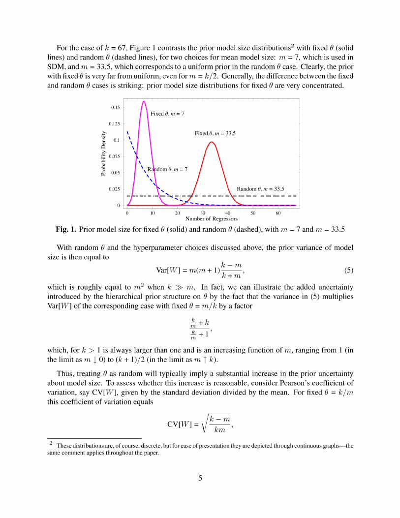
For the case of k = 67, Figure 1 contrasts the prior model size distributions2 with fixed θ (solidlines) and random θ (dashed lines), for two choices for mean model size: m = 7, which is used inSDM, and m = 33.5, which corresponds to a uniform prior in the random θ case. Clearly, the priorwith fixed θ is very far from uniform, even for m = k/2. Generally, the difference between the fixedand random θ cases is striking: prior model size distributions for fixed θ are very concentrated.

0 10 20 30 40 50 60Number of Regressors

0

0.025

0.05

0.075

0.1

0.125

0.15ProbabilityDensity

Fixed !, m " 7

Fixed !, m " 33.5

Random !, m " 7

Random !, m " 33.5

Fig. 1. Prior model size for fixed θ (solid) and random θ (dashed), with m = 7 and m = 33.5

With random θ and the hyperparameter choices discussed above, the prior variance of modelsize is then equal to

Var[W ] = m(m + 1)k −m

k + m, (5)

which is roughly equal to m2 when k � m. In fact, we can illustrate the added uncertaintyintroduced by the hierarchical prior structure on θ by the fact that the variance in (5) multipliesVar[W ] of the corresponding case with fixed θ = m/k by a factor

km + kkm + 1

,

which, for k > 1 is always larger than one and is an increasing function of m, ranging from 1 (inthe limit as m ↓ 0) to (k + 1)/2 (in the limit as m ↑ k).

Thus, treating θ as random will typically imply a substantial increase in the prior uncertaintyabout model size. To assess whether this increase is reasonable, consider Pearson’s coefficient ofvariation, say CV[W ], given by the standard deviation divided by the mean. For fixed θ = k/mthis coefficient of variation equals

CV[W ] =

√k −m

km,

2 These distributions are, of course, discrete, but for ease of presentation they are depicted through continuous graphs—thesame comment applies throughout the paper.

5

which is a rapidly decreasing function of m and is unity for m = k/(k + 1), which is often closeto one. Thus, for any reasonable prior mean model size, the prior with fixed θ will be far tootight. For example, if we take m = 7 in our applications, where k ranges from 41 to 67, CV[W ]will range from 0.344 to 0.358, which is quite small. For m = k/2, CV[W ] =

√1/k and ranges

from 0.122 to 0.156, clearly reflecting an unreasonable amount of precision in the prior model sizedistribution.

For random θ with the hyperprior as described above, we obtain

CV[W ] =

√(m + 1)(k −m)

m(k + m),

which is also decreasing in m, but is much flatter than the previous function over the rangeof practically relevant values for m.3 Taking m = 7 in our applications, CV[W ] will nowrange from 0.900 to 0.963, which is much more reasonable. For m = k/2, we now have thatCV[W ] =

√(k + 2)/3k, which ranges from 0.586 to 0.591.

Thus, this hierarchical prior seems quite a sensible choice. In addition, both Var[W ] and CV[W ]increase with k for a given m, which also seems a desirable property. This holds for both priorsettings; however, limk→∞ CV[W ] =

√(m + 1)/m for the case with random θ whereas this limit

is only√

1/m for the fixed θ case.

3.2. Prior odds

Posterior odds between any two models in M are given by

P (Mi|y)P (Mj |y)

=P (Mi)P (Mj)

· ly(Mi)ly(Mj)

,

where ly(Mi) is the marginal likelihood, which is discussed in the next subsection. Thus, the priordistribution on model space only affects posterior model inference through the prior odds ratioP (Mi)/P (Mj). For a prior with a fixed θ = 0.5 prior odds are equal to one (each model is a prioriequally probable). If we fix θ at a different value, these prior odds are

P (Mi)P (Mj)

=(

θ

1− θ

)ki−kj

,

thus inducing a prior penalty for the larger model if θ < 0.5 and favoring the larger model forvalues of θ > 0.5. Viewed in terms of the corresponding mean model size, m, we obtain (forθ = m/k):

P (Mi)P (Mj)

=(

m

k −m

)ki−kj

,

3 Of course, both CV functions tend to zero for m ↑ k since then all prior mass has to be on the full model. In addition,CV in both cases tends to∞ as m ↓ 0.

6

from which it is clear that the prior favors larger models if m > k/2. For the hierarchical Be(a, b)prior on θ, we obtain the prior model probabilities:

P (Mj) =∫ 1

0

P (Mj |θ)p(θ)dθ =Γ(a + b)Γ(a)Γ(b)

· Γ(a + kj)Γ(b + k − kj)Γ(a + b + k)

.

Using a = 1 and our prior elicitation in terms of E[W ] = m as above, we obtain the following priorodds

P (Mi)P (Mj)

=Γ(1 + ki) Γ

(k−m

m + k − ki

)Γ(1 + kj) Γ

(k−m

m + k − kj

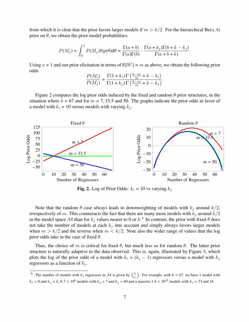
) .Figure 2 compares the log prior odds induced by the fixed and random θ prior structures, in the

situation where k = 67 and for m = 7, 33.5 and 50. The graphs indicate the prior odds in favor ofa model with ki = 10 versus models with varying kj .


!50!250255075100125

LogPriorOdds

Fixed "

m # 7

m # 33.5

m # 50


!30

!20

!10

0

10

20

LogPriorOdds

Random "

m # 7m # 33.5

m # 50

Fig. 2. Log of Prior Odds: ki = 10 vs varying kj

Note that the random θ case always leads to downweighting of models with kj around k/2,irrespectively of m. This counteracts the fact that there are many more models with kj around k/2in the model space M than for kj values nearer to 0 or k.4 In contrast, the prior with fixed θ doesnot take the number of models at each kj into account and simply always favors larger modelswhen m > k/2 and the reverse when m < k/2. Note also the wider range of values that the logprior odds take in the case of fixed θ.

Thus, the choice of m is critical for fixed θ, but much less so for random θ. The latter priorstructure is naturally adaptive to the data observed. This is, again, illustrated by Figure 3, whichplots the log of the prior odds of a model with ki = (kj − 1) regressors versus a model with kj

regressors as a function of kj .

4 The number of models with kj regressors in M is given by(

kkj

). For example, with k = 67, we have 1 model with

kj = 0 and kj = k, 8.7× 108 models with kj = 7 and kj = 60 and a massive 1.4× 1019 models with kj = 33 and 34.

7

10 20 30 40 50 60Number of Regressors

!1

0

1

2

LogPriorOdds

Fixed "m # 7

m # 33.5

m # 50


!4

!2

0

2

4

LogPriorOdds

Random "

m # 7

m # 33.5

m # 50

Fig. 3. Log of Prior Odds: ki = (kj − 1) vs varying kj

Whereas the fixed θ prior always favors the smaller model Mi for m < k/2, the choice of mfor random θ only moderately affects the prior odds, which swing towards the larger model whenkj gets larger than approximately k/2. This means that using the prior with fixed θ will have adeceptively strong impact on posterior model size. This prior does not allow for the data to adjustprior assumptions on mean model size that are at odds with the data, making it a much more riskychoice.

3.3. Bayes factors

In the previous subsection we mentioned the marginal likelihood, which is defined as the samplingdensity integrated out with the prior. The marginal likelihood forms the basis for the Bayes factor(ratio of marginal likelihoods) and can be derived analytically for each model with prior structure(2) on the model parameters. Provided g in (2) does not depend on the model size kj , the Bayesfactor for any two models from (1)–(2) becomes:

ly(Mi)ly(Mj)

=(

g

g + 1

) ki−kj2(

1 + g −R2i

1 + g −R2j

)−n−12

(6)

where R2i is the usual coefficient of determination for model Mi, i.e., R2

i = 1 − [y′QXiy/(y −

yιn)′(y − yιn)] and we have defined QA = I −A(A′A)−1A′ and Xi = (ιn, Zi), the design matrixof Mi, which is always assumed to be of full column rank. The expression in (6) is the relativeweight that the data assign to the corresponding models, and depends on sample size n, the factorg of the g-prior and the size and fit of both models, with the latter expressed through R2.

Let us compare this with the so-called BACE approach of SDM. The BACE approach is nottotally Bayesian, as it is not formally derived from a prior-likelihood specification, but relies onan approximation as sample size, n, goes to infinity (which may not be that realistic in the growthcontext). In fact, BACE uses the Schwarz approximation to compute the Bayes factor, as wasearlier used in Raftery (1995) in a very similar context. From equation (6) in SDM, we get the

8

following Bayes factor:

ly(Mi)ly(Mj)

= nkj−ki

2

(1−R2

i

1−R2j

)−n2

. (7)

This expression is not that different from the one in our equation (6), provided we take g = 1/n. Inthat case, the Bayes factor in (6) becomes:

ly(Mi)ly(Mj)

= (n + 1)kj−ki

2

(1 + 1

n −R2i

1 + 1n −R2

j

)−n−12

,

which behaves very similarly to the BACE procedure in (7) for practically relevant values of n (asin the examples here). This will be crucial in explaining the similarity of the results with the FLSand SDM prior settings mentioned before.

It also becomes immediately clear that the necessity of choosing prior settings implicit in usingBMA is not really circumvented by the use of BACE, in contrast with the claims in SDM. In fact,BACE implicitly fixes g in the context of our BMA framework. The fact that this is hidden tothe analyst does not make the results more robust with respect to this choice. It even carries asubstantial risk of conveying a false sense of robustness to the applied analyst.

Now we can examine more in detail how the various prior choices translate into model sizepenalties. From (6) we immediately see that if we have two models that fit equally well (i.e.,R2

i = R2j ), then the Bayes factor will approximately equal g(ki−kj)/2 (as g tends to be quite small).

If one of the models contains one more regressor, this means that the larger model will be penalizedby g1/2.

For n = 88 and k = 67 (as in the SDM data) this means that the choice of g = 1/n leads to aBayes factor of 0.107 and choosing g = 1/k2 implies a Bayes factor of 0.015. Thus, the model sizepenalty is much more severe for g = 1/k2 in the context of these types of data. The size penaltyimplicit in the BACE procedure is the same as for g = 1/n.

We can also ask how much data evidence is required to exactly compensate for the effects ofprior odds under different specifications. Posterior odds will be unity if the Bayes factor equals theinverse of the prior odds, thus if

ly(Mi)ly(Mj)

=P (Mj)P (Mi)

, (8)

where the prior odds are given in the previous subsection, as a function of prior mean model sizem, as well as k and the sizes of both models.

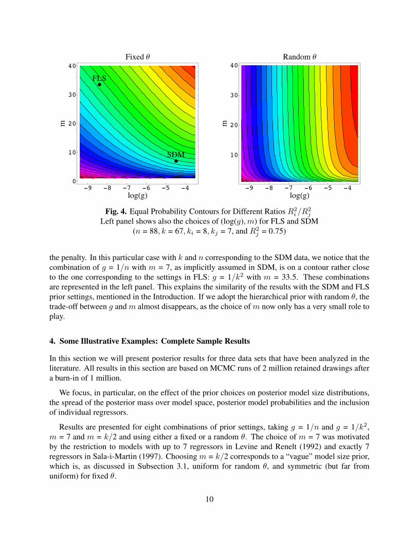
Typically, we have no control over n and k, but we do need to select g and m. To givemore insight into the tradeoff between g and m, Figure 4 plots the contours in (g,m)-space thatcorrespond to n = 88, k = 67, ki = 8, kj = 7, and R2

j = 0.75 for different ratios R2i /R2

j that wouldmake the two models equally probable in the posterior. These plots are provided for fixed andrandom θ model priors with the Bayes factor in (6).

It is obvious from the left figure for the fixed θ case that there is a clear trade-off between mand g: larger m, inducing a smaller size penalty, can be compensated by a small g, which increases

9

-9 -8 -7 -6 -5 -4log!g"0

10

20

30

40m

Fixed !

SDM

FLS

-9 -8 -7 -6 -5 -4log!g"

10

20

30

40

m

Random !

Fig. 4. Equal Probability Contours for Different Ratios R2i /R2

j

Left panel shows also the choices of (log(g),m) for FLS and SDM(n = 88, k = 67, ki = 8, kj = 7, and R2

j = 0.75)

the penalty. In this particular case with k and n corresponding to the SDM data, we notice that thecombination of g = 1/n with m = 7, as implicitly assumed in SDM, is on a contour rather closeto the one corresponding to the settings in FLS: g = 1/k2 with m = 33.5. These combinationsare represented in the left panel. This explains the similarity of the results with the SDM and FLSprior settings, mentioned in the Introduction. If we adopt the hierarchical prior with random θ, thetrade-off between g and m almost disappears, as the choice of m now only has a very small role toplay.

4. Some Illustrative Examples: Complete Sample Results

In this section we will present posterior results for three data sets that have been analyzed in theliterature. All results in this section are based on MCMC runs of 2 million retained drawings aftera burn-in of 1 million.

We focus, in particular, on the effect of the prior choices on posterior model size distributions,the spread of the posterior mass over model space, posterior model probabilities and the inclusionof individual regressors.

Results are presented for eight combinations of prior settings, taking g = 1/n and g = 1/k2,m = 7 and m = k/2 and using either a fixed or a random θ. The choice of m = 7 was motivatedby the restriction to models with up to 7 regressors in Levine and Renelt (1992) and exactly 7regressors in Sala-i-Martin (1997). Choosing m = k/2 corresponds to a “vague” model size prior,which is, as discussed in Subsection 3.1, uniform for random θ, and symmetric (but far fromuniform) for fixed θ.

10

4.1. The FLS Data

We first illustrate the effects of our prior choices using the growth data of FLS. The latter data setcontains k = 41 potential regressors to model the average per capita GDP growth over 1960-1992for a sample of n = 72 countries.5

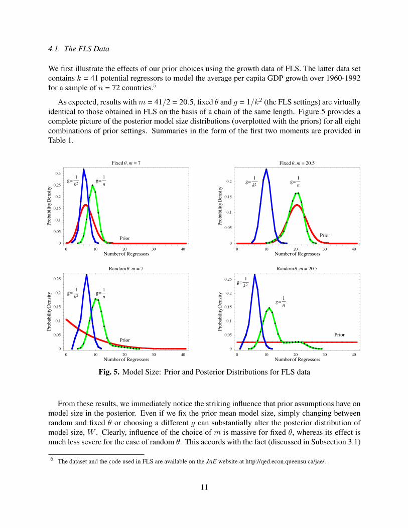
As expected, results with m = 41/2 = 20.5, fixed θ and g = 1/k2 (the FLS settings) are virtuallyidentical to those obtained in FLS on the basis of a chain of the same length. Figure 5 provides acomplete picture of the posterior model size distributions (overplotted with the priors) for all eightcombinations of prior settings. Summaries in the form of the first two moments are provided inTable 1.

0 10 20 30 40Numberof Regressors

0

0.05

0.1

0.15

0.2

0.25

ytilibaborPytisne

D

Randomq, m = 7

g= 1n

g= 1k2

Prior


0

0.05

0.1

0.15

0.2

0.25

ytilibaborPytisne

D

Randomq, m = 20.5

g= 1n

g=1k2

Prior


0

0.05

0.1

0.15

0.2

0.25

0.3

ytilibaborPytisne

D

Fixed q, m = 7

g= 1n

g= 1k2

Prior


0

0.05

0.1

0.15

0.2

ytilibaborPytisne

D

Fixed q, m = 20.5

g=1n

g=1k2

Prior

LS6 Fig6.nb 1

Printed by Mathematica for Students

Fig. 5. Model Size: Prior and Posterior Distributions for FLS data

From these results, we immediately notice the striking influence that prior assumptions have onmodel size in the posterior. Even if we fix the prior mean model size, simply changing betweenrandom and fixed θ or choosing a different g can substantially alter the posterior distribution ofmodel size, W . Clearly, influence of the choice of m is massive for fixed θ, whereas its effect ismuch less severe for the case of random θ. This accords with the fact (discussed in Subsection 3.1)

5 The dataset and the code used in FLS are available on the JAE website at http://qed.econ.queensu.ca/jae/.

11

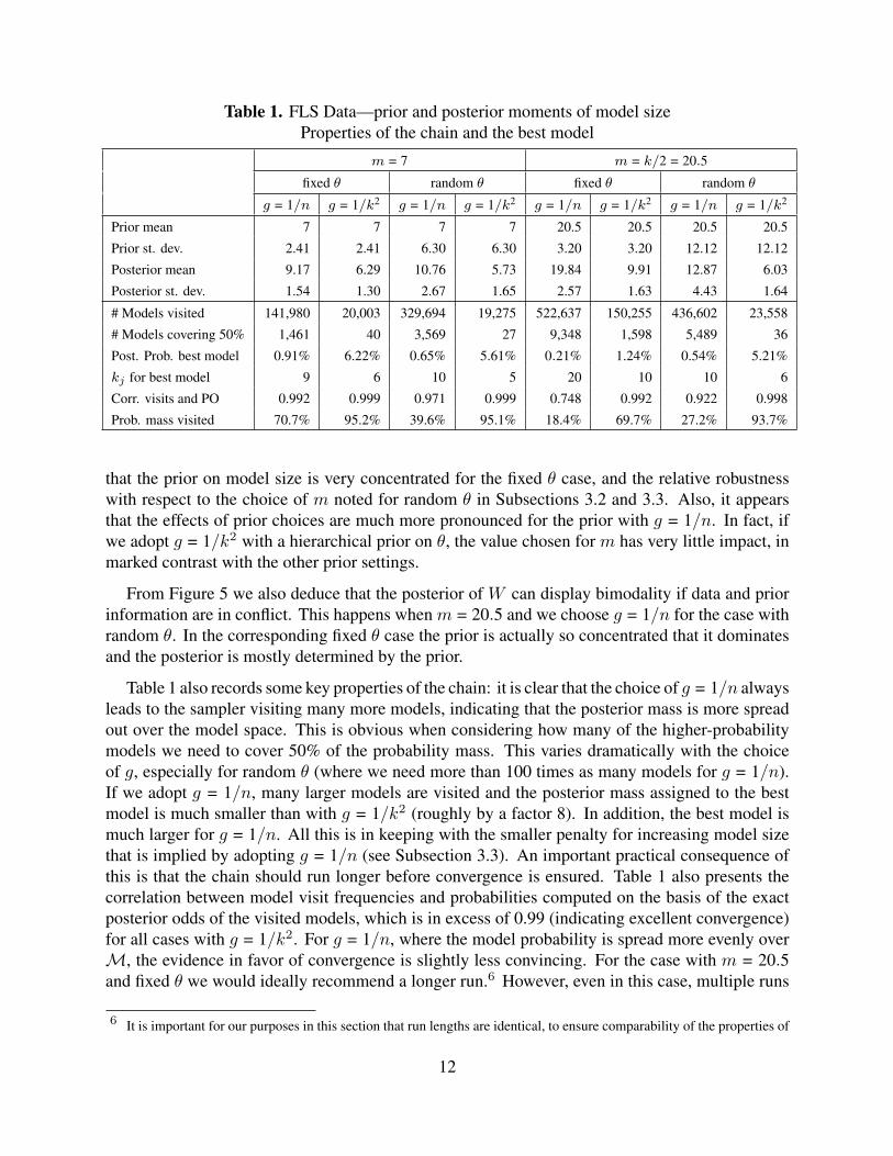
Table 1. FLS Data—prior and posterior moments of model sizeProperties of the chain and the best model

m = 7 m = k/2 = 20.5

fixed θ random θ fixed θ random θ

g = 1/n g = 1/k2 g = 1/n g = 1/k2 g = 1/n g = 1/k2 g = 1/n g = 1/k2

Prior mean 7 7 7 7 20.5 20.5 20.5 20.5

Prior st. dev. 2.41 2.41 6.30 6.30 3.20 3.20 12.12 12.12

Posterior mean 9.17 6.29 10.76 5.73 19.84 9.91 12.87 6.03

Posterior st. dev. 1.54 1.30 2.67 1.65 2.57 1.63 4.43 1.64

# Models visited 141,980 20,003 329,694 19,275 522,637 150,255 436,602 23,558

# Models covering 50% 1,461 40 3,569 27 9,348 1,598 5,489 36

Post. Prob. best model 0.91% 6.22% 0.65% 5.61% 0.21% 1.24% 0.54% 5.21%

kj for best model 9 6 10 5 20 10 10 6

Corr. visits and PO 0.992 0.999 0.971 0.999 0.748 0.992 0.922 0.998

Prob. mass visited 70.7% 95.2% 39.6% 95.1% 18.4% 69.7% 27.2% 93.7%

that the prior on model size is very concentrated for the fixed θ case, and the relative robustnesswith respect to the choice of m noted for random θ in Subsections 3.2 and 3.3. Also, it appearsthat the effects of prior choices are much more pronounced for the prior with g = 1/n. In fact, ifwe adopt g = 1/k2 with a hierarchical prior on θ, the value chosen for m has very little impact, inmarked contrast with the other prior settings.

From Figure 5 we also deduce that the posterior of W can display bimodality if data and priorinformation are in conflict. This happens when m = 20.5 and we choose g = 1/n for the case withrandom θ. In the corresponding fixed θ case the prior is actually so concentrated that it dominatesand the posterior is mostly determined by the prior.

Table 1 also records some key properties of the chain: it is clear that the choice of g = 1/n alwaysleads to the sampler visiting many more models, indicating that the posterior mass is more spreadout over the model space. This is obvious when considering how many of the higher-probabilitymodels we need to cover 50% of the probability mass. This varies dramatically with the choiceof g, especially for random θ (where we need more than 100 times as many models for g = 1/n).If we adopt g = 1/n, many larger models are visited and the posterior mass assigned to the bestmodel is much smaller than with g = 1/k2 (roughly by a factor 8). In addition, the best model ismuch larger for g = 1/n. All this is in keeping with the smaller penalty for increasing model sizethat is implied by adopting g = 1/n (see Subsection 3.3). An important practical consequence ofthis is that the chain should run longer before convergence is ensured. Table 1 also presents thecorrelation between model visit frequencies and probabilities computed on the basis of the exactposterior odds of the visited models, which is in excess of 0.99 (indicating excellent convergence)for all cases with g = 1/k2. For g = 1/n, where the model probability is spread more evenly overM, the evidence in favor of convergence is slightly less convincing. For the case with m = 20.5and fixed θ we would ideally recommend a longer run.6 However, even in this case, multiple runs

6 It is important for our purposes in this section that run lengths are identical, to ensure comparability of the properties of

12

led to very similar findings. For completeness, Table 1 also displays the estimated total posteriormodel probability visited by the chain, computed as suggested in George and McCulloch (1997).

For the random θ cases, the specification and the posterior probability of the best model is notmuch affected by the choice of m. However, changing from g = 1/n to g = 1/k2 has a dramaticeffect on both.

Finally, the size of the best model varies in between 5 and 20, and is not much affected by mfor random θ.

Of course, one of the main reasons for using BMA in the first place is to assess which of theregressors are important for modelling growth. Table 2 presents the marginal posterior inclusionprobabilities of all regressors that receive an inclusion probability of over 10% under any of theprior settings. It is clear that there is a large amount of variation in which regressors are identifiedas important, depending on the prior assumptions.

Whereas three variables (past GDP, fraction Confucian and Equipment investment) receive morethan 0.75 inclusion probability and a further two (Life expectancy and the Sub-Saharan dummy)are included with at least probability 0.50 in all cases, there are many differences. If we comparecases that only differ in m, the choice of g = 1/n with fixed θ leads to dramatic differences ininclusion probabilities: Fraction Hindu, the Labour force size, and Higher education enrollmentgo from virtually always included with m = 20.5 to virtually never included with m = 7; theNumber of years open economy has the seventh largest inclusion probability for m = 7 and dropsto the bottom of the 32 variables shown in the table for m = 20.5. In sharp contrast, the case withg = 1/k2 and random θ leads to very similar inclusion probabilities for both values of m.

Finally, note that results for model size, chain behavior and inclusion probabilities are quitesimilar for the cases where g = 1/n with fixed θ = 7/41 (the preferred implied prior in SDM) andwhere g = 1/k2 with θ = 0.5 (the prior used in FLS). This is in line with the negative trade-offbetween g and m illustrated in Figure 4, which explains the similarity between empirical resultsusing BACE and the FLS prior on the same data. The same behavior is observed for the otherdatasets presented in the next subsections.

4.2. The Data Set of MP

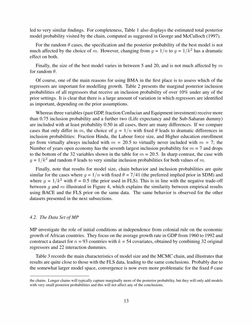
MP investigate the role of initial conditions at independence from colonial rule on the economicgrowth of African countries. They focus on the average growth rate in GDP from 1960 to 1992 andconstruct a dataset for n = 93 countries with k = 54 covariates, obtained by combining 32 originalregressors and 22 interaction dummies.

Table 3 records the main characteristics of model size and the MCMC chain, and illustrates thatresults are quite close to those with the FLS data, leading to the same conclusions. Probably due tothe somewhat larger model space, convergence is now even more problematic for the fixed θ case

the chains. Longer chains will typically capture marginally more of the posterior probability, but they will only add modelswith very small posterior probabilities and this will not affect any of the conclusions.

13

Table 2. FLS data—Marginal posterior inclusion probabilities of the covariatesm = 7 m = k/2 = 20.5

fixed θ random θ fixed θ random θRegressors g = 1/n g = 1/k2 g = 1/n g = 1/k2 g = 1/n g = 1/k2 g = 1/n g = 1/k2

log GDP in 1960 1.00 0.91 1.00 0.79 1.00 1.00 1.00 0.84

Fraction Confucian 0.99 0.94 1.00 0.93 1.00 1.00 1.00 0.94

Life expectancy 0.92 0.74 0.95 0.63 1.00 0.95 0.97 0.68

Equipment investment 0.95 0.98 0.93 0.98 0.97 0.94 0.94 0.98

Sub-Saharan dummy 0.70 0.59 0.78 0.53 1.00 0.75 0.85 0.55

Fraction Muslim 0.62 0.29 0.63 0.23 0.43 0.66 0.61 0.27

Rule of law 0.41 0.17 0.56 0.15 0.93 0.52 0.67 0.17

Number of years open economy 0.56 0.60 0.46 0.54 0.07 0.50 0.36 0.56

Degree of capitalism 0.36 0.09 0.50 0.08 0.56 0.47 0.56 0.09

Fraction Protestant 0.38 0.23 0.49 0.24 0.47 0.46 0.51 0.24

Fraction GDP in mining 0.36 0.08 0.51 0.07 0.94 0.44 0.63 0.08

Non-Equipment investment 0.33 0.07 0.47 0.06 0.71 0.43 0.56 0.07

Latin American dummy 0.18 0.09 0.23 0.07 0.75 0.19 0.34 0.08

Primary school enrollment, 1960 0.19 0.10 0.21 0.08 0.63 0.18 0.29 0.09

Fraction Buddhist 0.14 0.05 0.20 0.07 0.25 0.17 0.23 0.07

Black market premium 0.11 0.02 0.22 0.01 0.69 0.16 0.34 0.02

Fraction Catholic 0.09 0.03 0.13 0.02 0.12 0.11 0.14 0.03

Civil liberties 0.09 0.03 0.13 0.02 0.54 0.10 0.22 0.03

Fraction Hindu 0.06 0.07 0.18 0.01 0.97 0.10 0.36 0.01

Political rights 0.06 0.01 0.09 0.01 0.29 0.07 0.13 0.02

Exchange rate distortions 0.06 0.03 0.06 0.02 0.12 0.06 0.08 0.03

Age 0.06 0.02 0.07 0.02 0.25 0.06 0.10 0.02

War dummy 0.05 0.02 0.06 0.02 0.14 0.05 0.08 0.02

Fraction of Pop. Speaking English 0.04 0.01 0.07 0.01 0.42 0.05 0.15 0.01

Size labor force 0.04 0.01 0.11 0.01 0.95 0.05 0.28 0.01

Ethnolinguistic fractionalization 0.03 0.01 0.09 0.01 0.87 0.03 0.24 0.01

Spanish Colony dummy 0.03 0.01 0.06 0.01 0.59 0.03 0.17 0.01

French Colony dummy 0.03 0.01 0.05 0.01 0.54 0.03 0.15 0.01

Higher education enrollment 0.02 0.01 0.08 0.01 0.91 0.02 0.24 0.01

British colony dummy 0.02 0.00 0.04 0.00 0.47 0.02 0.13 0.00

Outward orientation 0.02 0.01 0.04 0.01 0.42 0.02 0.12 0.01

Public education share 0.02 0.00 0.03 0.00 0.30 0.02 0.08 0.00

with g = 1/n and m = 54/2 = 27. Again, however, longer runs do not lead to appreciably differentconclusions (see footnote 6).

4.3. The Data Set of SDM and DW

SDM and Doppelhofer and Weeks (2006) use a larger data set, and model annual GDP growth percapita between 1960 and 1996 for n = 88 countries as a function of k = 67 potential drivers.7

Despite the larger model space (the number of models in M is now 1.5× 1020), Table 4 showsthat posterior model probabilities are more concentrated than in the previous two cases; in fact,even in those cases where many models are visited, 50% of the posterior mass is still accounted forthrough a rather small number of models. Also, model sizes tend to be smaller; in fact, the posteriormean model size is less than 3 for three of the four cases with g = 1/k2. If we adopt a random

7 The data and the code used in SDM are available at http://www.econ.cam.ac.uk/faculty/doppelhofer/

14

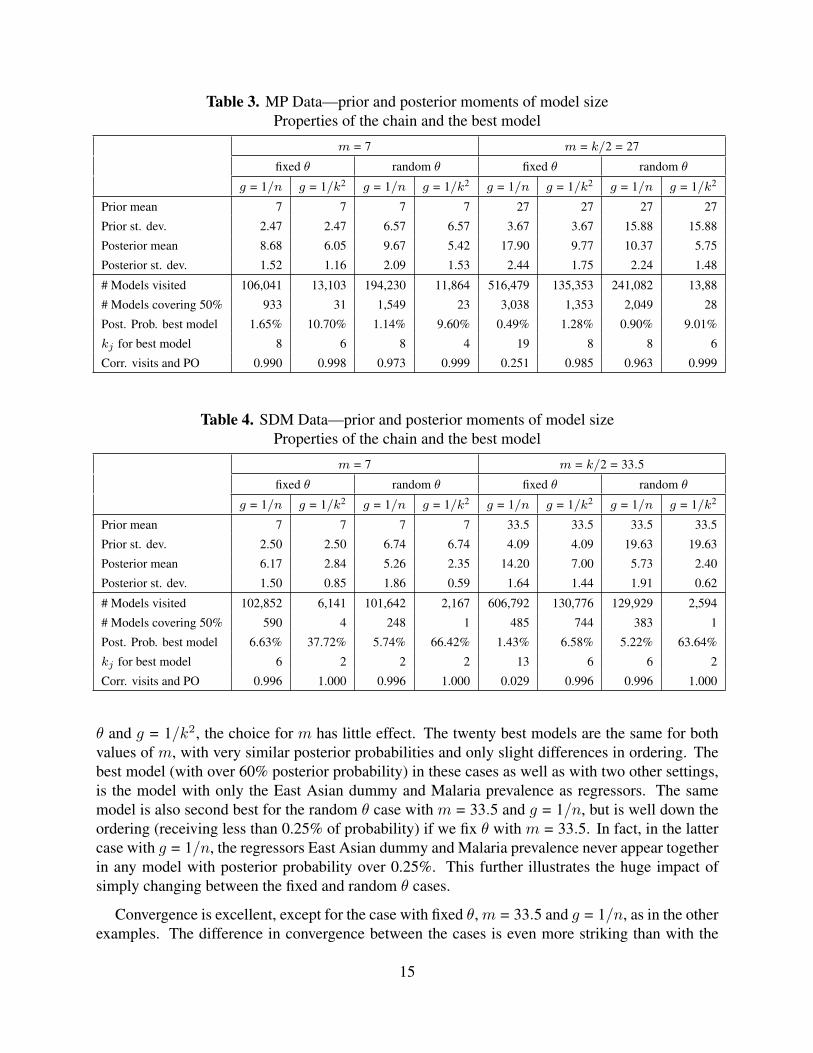
Table 3. MP Data—prior and posterior moments of model sizeProperties of the chain and the best model

m = 7 m = k/2 = 27



Prior mean 7 7 7 7 27 27 27 27

Prior st. dev. 2.47 2.47 6.57 6.57 3.67 3.67 15.88 15.88

Posterior mean 8.68 6.05 9.67 5.42 17.90 9.77 10.37 5.75

Posterior st. dev. 1.52 1.16 2.09 1.53 2.44 1.75 2.24 1.48

# Models visited 106,041 13,103 194,230 11,864 516,479 135,353 241,082 13,88

# Models covering 50% 933 31 1,549 23 3,038 1,353 2,049 28


kj for best model 8 6 8 4 19 8 8 6


Table 4. SDM Data—prior and posterior moments of model sizeProperties of the chain and the best model

m = 7 m = k/2 = 33.5



Prior mean 7 7 7 7 33.5 33.5 33.5 33.5

Prior st. dev. 2.50 2.50 6.74 6.74 4.09 4.09 19.63 19.63

Posterior mean 6.17 2.84 5.26 2.35 14.20 7.00 5.73 2.40

Posterior st. dev. 1.50 0.85 1.86 0.59 1.64 1.44 1.91 0.62

# Models visited 102,852 6,141 101,642 2,167 606,792 130,776 129,929 2,594

# Models covering 50% 590 4 248 1 485 744 383 1


kj for best model 6 2 2 2 13 6 6 2


θ and g = 1/k2, the choice for m has little effect. The twenty best models are the same for bothvalues of m, with very similar posterior probabilities and only slight differences in ordering. Thebest model (with over 60% posterior probability) in these cases as well as with two other settings,is the model with only the East Asian dummy and Malaria prevalence as regressors. The samemodel is also second best for the random θ case with m = 33.5 and g = 1/n, but is well down theordering (receiving less than 0.25% of probability) if we fix θ with m = 33.5. In fact, in the lattercase with g = 1/n, the regressors East Asian dummy and Malaria prevalence never appear togetherin any model with posterior probability over 0.25%. This further illustrates the huge impact ofsimply changing between the fixed and random θ cases.

Convergence is excellent, except for the case with fixed θ, m = 33.5 and g = 1/n, as in the otherexamples. The difference in convergence between the cases is even more striking than with the

15

previous examples, and it appears that the case with convergence problems struggles to adequatelydescribe the posterior distribution on the model space M. While most of the mass is covered bya relatively small number of models, the prior assumptions induce a very fat tail of models withlittle but nonnegligible mass. However, inference on most things of interest, such as the regressorinclusion probabilities is not much affected by running longer chains. For all other prior settings,the very large model space is remarkably well explored by the MCMC chain.

5. Robustness and Predictive Analysis: Results from 100 Subsamples

In the previous section we have illustrated that the choice of, perhaps seemingly innocuous, priorsettings can have a dramatic impact on the posterior inference resulting from BMA. Posterior modelprobabilities and identification of the most important regressors can strongly depend on the priorsettings we use in our analysis of growth regressions through BMA.

We now address the issue of whether small changes to the data set would result in large changesin inference—i.e., data robustness. In addition, we want to assess the predictive performance of themodel under various prior settings. We will use the same device to investigate both issues, namelythe partition of the available data into an inference subsample and a prediction subsample. We willthen use the various inference subsamples for the evaluation of robustness and assess predictionon the basis of how well the predictive distribution based on the inference subsamples captures thecorresponding prediction subsamples.

We take random partitions of the sample, where the size of the prediction subsample is fixedat 15% of the total number of observations (rounded to an integer), leaving 85% of the sampleto conduct inference with. We generate random prediction subsamples of a fixed size by usingthe algorithm of McLeod and Bellhouse (1983). We use 100 random partitions and compute theposterior results through an MCMC chain of 500,000 drawings with a burn-in of 100,000 for eachpartition. This led to excellent convergence, with the exception of the cases with θ fixed at 0.5 andg = 1/n. Thus, for this combination we have used a chain of length 1,000,000 after a burn-in of500,000, which leads to reliable results.8 To increase comparability, we use the same partitions forall prior settings.

5.1. Robustness

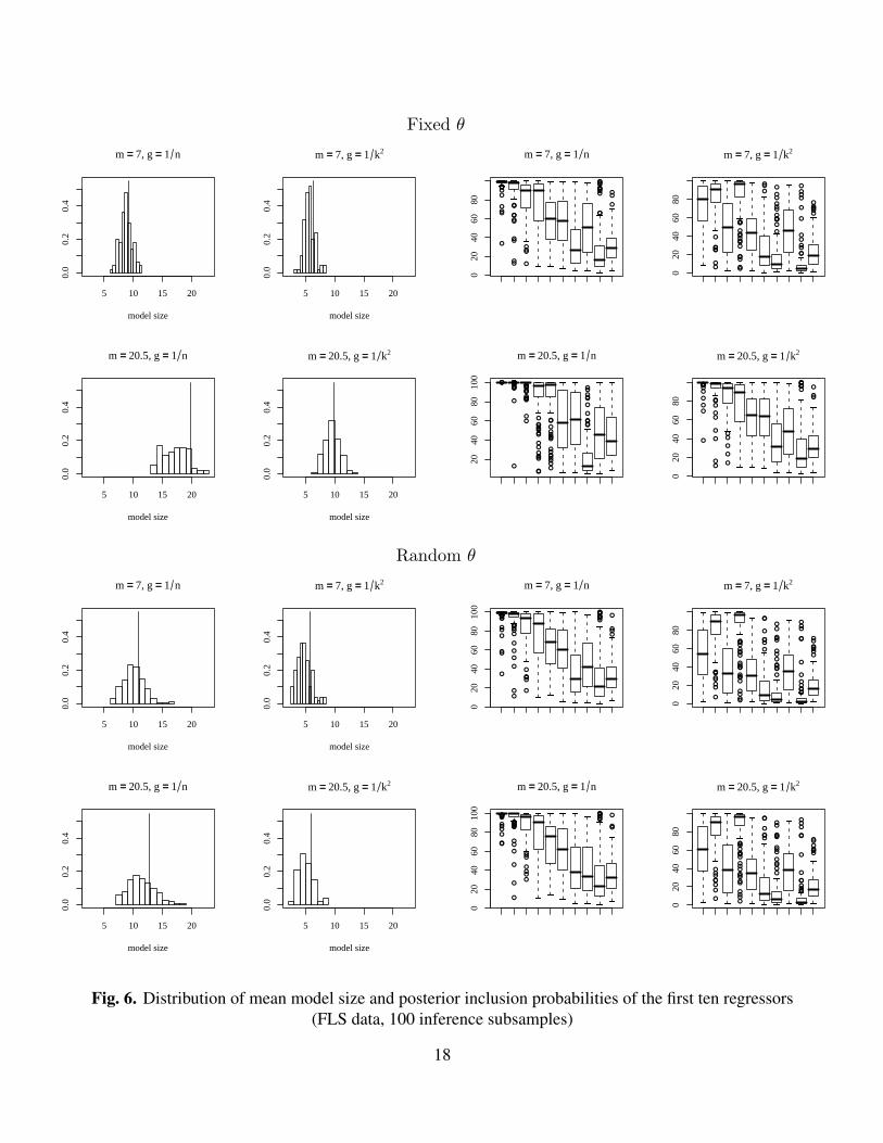
Figure 6 indicates the distribution of the posterior mean model size across 100 inference subsamplesof the FLS data (left panel). Values corresponding to the full sample are indicated by verticallines. The right panel of the same Figure shows the posterior inclusion probabilities of the tenregressors with highest posterior inclusion probabilities in the full-sample analysis with the FLSprior setting—i.e., θ = 0.5 and g = 1/ max{n, k2}.

A striking characteristic of both panels is the sensitivity of the results to the choice of m for thefixed θ priors, whereas the effect of m is very small for the cases with random θ. The choice of g,

8 In fact, the results are very close to those obtained with 100,000 burn-in and 500,000 retained drawings, with the onlynoticeable difference in the maximum LPS values.

16

however, always matters: g = 1/k2 generally leads to smaller mean model sizes and results in verydifferent conclusions on which regressors are important than g = 1/n, especially for random θ.

Given each choice of prior, the results vary quite a bit across subsamples, especially for theinclusion probabilities where the interquartile ranges can be as high as 60%. It is interesting how thecombinations of g = 1/n with fixed θ = 7/41 (the setting implicitly favored in SDM) and g = 1/k2

with θ = 0.5 (the prior of FLS) lead to very similar results, both for model sizes and inclusionprobabilities, as also noted in Section 4. Overall, the difference between fixed and random θ casesis small for m = 7, but substantial for m = k/2.

For the MP data, results on posterior model size are quite similar as for the FLS dataset, and wecan draw the same conclusions on the basis of the inclusion probabilities.

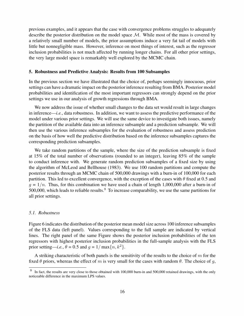
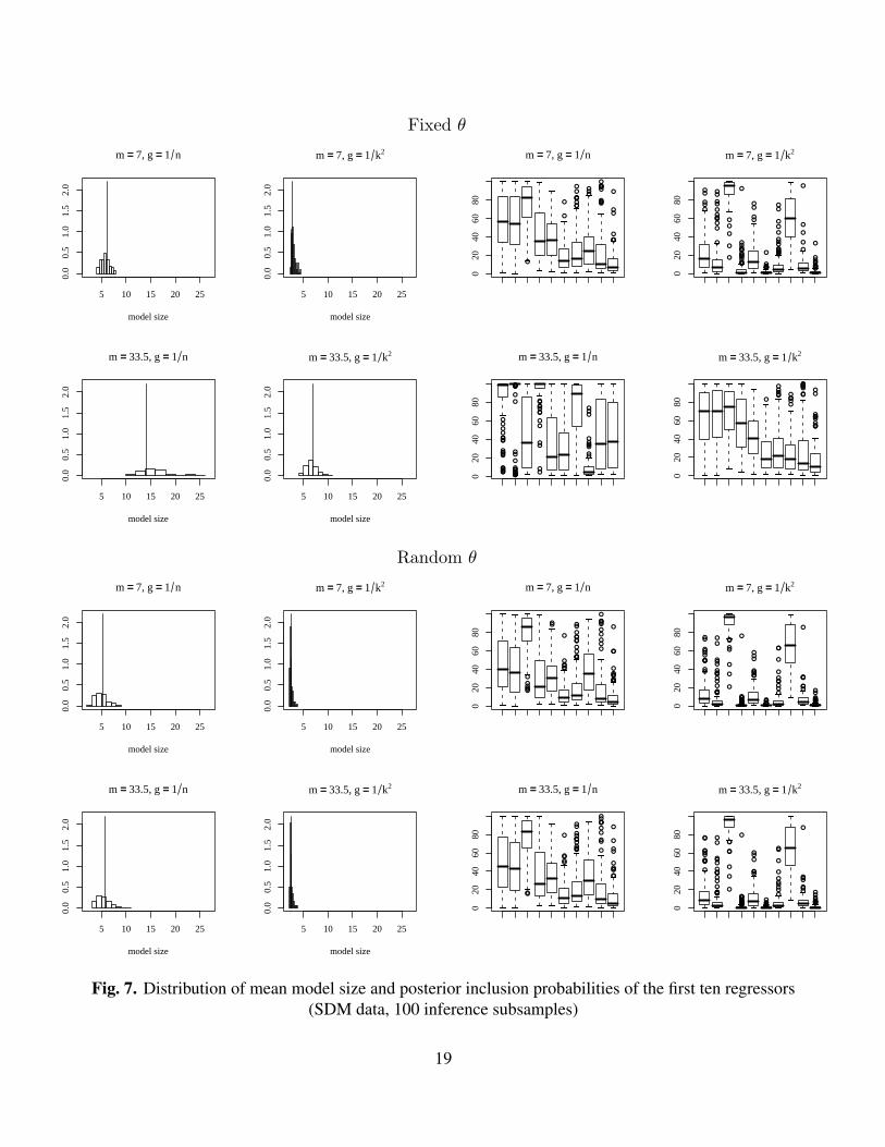
Finally, Figure 7 shows the robustness results for the SDM data set, where we have k = 67potential regressors. As before, the choice of m critically affects the fixed θ results, but not theones for random θ. Differences between fixed and random θ cases are large for m = k/2, butrelatively small for m = 7, as with both previous datasets. Again, the choice of g always affectsthe results, and inference using g = 1/n in combination with θ = 7/67 is quite similar to that usingg = 1/k2 with θ = 0.5, for both model size and inclusion probabilities. For g = 1/k2 inference onmodel size is quite concentrated on small values, with the exception of the case with fixed θ andm = 33.5.

Even though many results are not very robust with respect to the particular choice of subsample,it is clear that the differences induced by the various prior assumptions largely persist if we takeinto account small changes to the data.

17

Fixed θ

m == 7, g == 1 n

model size

5 10 15 20

0.0

0.2

0.4

m == 7, g == 1 k2

model size

5 10 15 20

0.0

0.2

0.4

m == 20.5, g == 1 n

model size

5 10 15 20

0.0

0.2

0.4

m == 20.5, g == 1 k2

model size

5 10 15 20

0.0

0.2

0.4

●

●●

●

●●

●●

●

●

●

●

●

●

●

●

●

●

●

●

●●●

●

●

●

●

●

●

●●●

●●●●

●

●

020

4060

80

m == 7, g == 1 n

●

●

●●●

●

●●

●

●

●

●

●

●

●●

●

●

●

●

●●

●●●

●

●●

●

●

●●

●●

●

●

●

●

●

●●

●

●

●●

●

●

●

●

●●●●●

●

020

4060

80

m == 7, g == 1 k2

●●●●●●●●●

●

●●

●

●●●●●●●●●●● ●

●●

●

●

●●●

●●

●

●

●

●

●

●

●●

●

●

●●

●

●

●

●

●

●

●

●

●●

●●

●

●

●

●

●

●

●●

●

●

●

●

●

●

●

●

●

●●

●

●

●

●

2040

6080

100

m == 20.5, g == 1 n

●

●●●●

●

●●

●

●

●

●

●

●●

●

●

●

●

●

●

●

●

●●

●

●

●●

●

●●●●●● ●

●●

020

4060

80

m == 20.5, g == 1 k2

Random θ

m == 7, g == 1 n

model size

5 10 15 20

0.0

0.2

0.4

m == 7, g == 1 k2

model size

5 10 15 20

0.0

0.2

0.4

m == 20.5, g == 1 n

model size

5 10 15 20

0.0

0.2

0.4

m == 20.5, g == 1 k2

model size

5 10 15 20

0.0

0.2

0.4

●

●●●

●

●

●

●●

●

●

●

●●

●

●

●

●

●

●

●

●

●

●

●

●

●●

●

●●

●

●●●●●● ●

●●●

020

4060

8010

0

m == 7, g == 1 n

●

●

●

●●

●

●

●

●

●

●

●

●

●

●

●

●

●

●

●

●

●●

●

●

●

●

●

●●

●●

●

●

●

●●

●

●

●

●

●

●

●

●

●●

● ●

●

●

●●

●

●

●

●●

●

●

●

●●

●

●

●

●●

020

4060

80

m == 7, g == 1 k2

●

●●●

●

●●

●●

●

●

●

●●●

●

●

●

●●

●

●

●

●

●

●

●

●

●

●

●

●●

●

●●●●●●●● ●

●●

020

4060

8010

0

m == 20.5, g == 1 n

●

●

●●●

●

●

●

●

●

●

●

●

●

●

●

●

●

●

●

●

●

●

●

●

●

●

●

●●

●●

●

●

●●

●

●

●

●

●

●

●●

●●

● ●

●

●

●●

●

●

●●

●

●

●

●

●●

●

●

●

●●

020

4060

80

m == 20.5, g == 1 k2

1

Fig. 6. Distribution of mean model size and posterior inclusion probabilities of the first ten regressors(FLS data, 100 inference subsamples)

18

Fixed θ

m == 7, g == 1 n

model size

5 10 15 20 25

0.0

0.5

1.0

1.5

2.0

m == 7, g == 1 k2

model size

5 10 15 20 25

0.0

0.5

1.0

1.5

2.0

m == 33.5, g == 1 n

model size

5 10 15 20 25

0.0

0.5

1.0

1.5

2.0

m == 33.5, g == 1 k2

model size

5 10 15 20 25

0.0

0.5

1.0

1.5

2.0

●

●

●

●

●●

●●

●●

●

●●●

●●

●●●●

●●

●●

●

●

●●

●●

●

020

4060

80

m == 7, g == 1 n

●

●●

●● ●

●

●

●●

●

●

●●●

●

●

●

●

●

●

● ●

●

●

●

●

●

●●

●

●

●

●●●

●

●

●

●

●●●●●

●

●●●●

●●●

●

●●

●

●

●

●●

●

●

●●

●

●

●

●

●

●

●●●

●●

●

●●

●

●

020

4060

80

m == 7, g == 1 k2

●●●

●●●

●

●

●

●●

●●

●●

●

●

●

●

●

●

●

●

●

●

●

●

●●●●●●

●

●

●●

●●

●

●

●●

●

●

●

●●

●

●

●

●

●

●

●

●

●

●

●

●●

●●

●

●

●

020

4060

80

m == 33.5, g == 1 n

●

●●

●●●●●

●●●

●

●●●●

●

●●

●

●

●

●

●

●

●

●●●

●

020

4060

80

m == 33.5, g == 1 k2

Random θ

m == 7, g == 1 n

model size

5 10 15 20 25

0.0

0.5

1.0

1.5

2.0

m == 7, g == 1 k2

model size

5 10 15 20 25

0.0

0.5

1.0

1.5

2.0

m == 33.5, g == 1 n

model size

5 10 15 20 25

0.0

0.5

1.0

1.5

2.0

m == 33.5, g == 1 k2

model size

5 10 15 20 25

0.0

0.5

1.0

1.5

2.0

●

●●●●●

●●

●●●

●

●●

●

●

●●

●

●

●

●●

●●●

● ●●

●

●

●

●●

●

●●

●

●

●

●

●

●

●

●●●

●

020

4060

80

m == 7, g == 1 n

●

●●

●

●

●

●

●

●

●

●●

●

●

●

●

●●

●

●

●

●●●

●

●

●

●

●

●

●

●

●

●

●●●

●

●

●●●●●●●●●●●●●

●●

●●

●●●

●

●●●●●●●●●●●

●●

●

●

●

●

●●

●●

●

●

●

●●

●●

●●●

●●●●●●

●

●

020

4060

80

m == 7, g == 1 k2

●●

●

●

●

●●

●

●●

●

●

●

●●

●●●

● ●

●

●

●

●

●●

●

●●

●

●

●

●

●

●

●●

●

●

020

4060

80

m == 33.5, g == 1 n

●

●●

●

●

●

●

●

●

●

●

●

●

●

●

●●

●

●

●

●●●

●

●

●

●

●

●

●

●

●

●

●●●

●

●

●●●●●●●●●●●●

●

●●

●●

●

●●●●●●

●●●●●

●●

●

●

●

●

●●

●●

●

●

●

●●

●●

●●●

●●●●●●

●

●

020

4060

80

m == 33.5, g == 1 k2

1

Fig. 7. Distribution of mean model size and posterior inclusion probabilities of the first ten regressors(SDM data, 100 inference subsamples)

19

5.2. Prediction

In order to compare the predictive performance associated with the various prior choices, we turnnow to the task of predicting the observable, growth, given the regressors. Of course, the predictivedistribution is also derived through model averaging, as explained in, e.g., FLS. As a measure ofhow well each model predicts the retained observations, we use the log predictive score, which isa strictly proper scoring rule, described in FLS. In the case of i.i.d. sampling, LPS can be given aninterpretation in terms of the Kullback-Leibler divergence between the actual sampling density andthe predictive density (see Fernandez et al. 2001a), and smaller values indicate better predictionperformance.

We compare the predictions based on: (i) BMA, (ii) the best model (the model with the highestposterior probability), (iii) the full model (with all k regressors), and (iv) the null model (with onlythe intercept).

Panel A in Table 5 summarizes our findings for the FLS data: the entries indicating “best” or“worst” model or how often a model is beaten by the null are expressed in percentages of the 100samples for that particular prior setting.

(i) BMA—The predictive performance of BMA is much superior to that of the other procedures—which corroborates evidence in e.g. Raftery et al., 1997, Fernandez et al., 2001a and FLS. Itis never the worst predictor and leads to the best predictions in more than half of the sampledcases (with the exception of the prior with fixed θ = 0.5 and g = 1/n).

(ii) Best—Basing predictions solely on the model with highest posterior probability is clearly a lotworse: it almost never gives the best prediction and leads to the worst prediction in 18 to 46%of the cases; moreover, it is beaten by the simple null model in more than 35% of the cases.

(iii) Full—The use of the full model can lead to good forecasts, but is very risky, as it also has asubstantial probability of delivering the worst performance: in fact, for g = 1/k2 the proportionof the latter always exceeds the fraction of best performances. This behavior is also illustratedby the fact that {Min, Mean, Max} for LPS of the full model is {0.74, 1.77, 3.77} for g = 1/nand {0.67, 2.15, 5.82} for g = 1/k2. For comparison, the null model leads to {1.67, 2.05, 2.72}.

Having established that BMA is the strategy to adopt for prediction, we can focus on the forecastperformance of BMA to compare the predictive ability across the different prior settings. Meanvalues of LPS (over all 100 samples) are not that different, but the maximum values indicate thatfixing θ at 0.5 is the most risky strategy. This suggests using random θ. In addition, BMA alwaysperforms better with respect to the other prediction strategies for g = 1/k2. Indeed, the worst casescenario for BMA appears to be θ = 0.5 with g = 1/n. Finally, the choice of m almost leaves therandom θ results unaffected, but has a substantial effect on the cases with fixed θ, in line with ourexpectations.

Panel B in Table 5 presents the same quantities for the MP data (where k = 54), and the{Min, Mean, Max} values for LPS of the full model are {1.13, 2.55, 6.05} for g = 1/n and{1.12, 2.79, 7.48} for g = 1/k2, whereas the null model leads to {1.70, 2.03, 2.63}.

The superiority of BMA is even more pronounced, with the prior setting θ = 0.5 with g = 1/nagain being the least favorable for BMA. The performance of the full model is now considerably

20

Table 5. Predictive performance: Three datasets (100 subsamples)Panel A. FLS Data

m = 7 m = k/2



Best 59 65 54 66 48 63 54 67

BMA Worst 0 0 0 0 0 0 0 0

(%) Beaten by Null 7 6 11 6 19 11 11 6

Best 1 2 1 0 3 2 2 0

Best model Worst 28 18 34 18 46 31 36 17

(%) Beaten by null 35 35 41 36 52 47 45 36

Best 34 28 37 30 37 24 36 29

Full model Worst 16 42 15 41 8 31 15 42

(%) Beaten by null 25 45 25 45 25 45 25 45

Minimum 1.12 1.19 1.12 1.21 0.86 1.11 1.11 1.20

LPS of BMA Mean 1.58 1.61 1.61 1.64 1.65 1.63 1.61 1.63

Maximum 2.57 2.52 2.67 2.53 2.76 2.85 2.64 2.47

St. dev. 0.30 0.26 0.33 0.25 0.42 0.37 0.34 0.25

Panel B. MP Data

Best 71 70 75 73 61 78 73 72

BMA Worst 0 0 0 0 0 0 0 1

(%) Beaten by null 15 16 15 18 32 15 16 18

Best 10 8 7 2 2 5 7 3

Best model Worst 18 4 19 6 37 18 20 5

(%) Beaten by null 42 35 42 33 63 49 43 31

Best 4 7 3 9 6 2 4 9

Full model Worst 61 75 59 75 46 66 59 75

(%) Beaten by null 71 77 71 77 71 77 71 77

Minimum 1.15 1.30 1.14 1.39 1.05 1.12 1.13 1.38

LPS of BMA Mean 1.70 1.74 1.71 1.77 1.87 1.72 1.72 1.77

Maximum 3.34 3.46 3.26 3.53 3.60 3.31 3.23 3.54

St. dev. 0.39 0.37 0.40 0.35 0.51 0.42 0.40 0.36

Panel C. SDM Data

Best 69 53 64 48 48 63 66 46

BMA Worst 0 0 0 0 0 0 0 0

(%) Beaten by null 15 11 16 10 51 16 16 10

Best 16 36 20 42 1 21 18 44

Best model Worst 3 1 3 0 12 2 3 0

(%) Beaten by null 38 20 31 19 79 39 32 18

Best 0 0 0 0 0 0 0 0

Full model Worst 97 99 97 100 88 98 97 100

(%) Beaten by null 99 100 99 100 99 100 99 100

Minimum 1.36 1.41 1.39 1.43 1.22 1.33 1.38 1.43

LPS of BMA Mean 1.78 1.75 1.78 1.75 2.18 1.81 1.79 1.74

Maximum 3.38 2.67 3.31 2.53 3.70 3.63 3.38 2.51

St. dev. 0.34 0.26 0.32 0.25 0.60 0.38 0.34 0.25

21

worse than for the FLS data, as this model quite often leads to the worst behavior and is soundlybeaten by the much more conservative null model. This seems in line with the fact that the numberof regressors, k, is now larger, so the full model is even more overparameterized than in the FLScase. Considering the LPS values for BMA, priors with g = 1/n seem to have a slight edge, exceptfor the case with a fixed θ = 0.5. Finally, the choice of m is again virtually immaterial for therandom θ cases, and affects those with fixed θ.

Finally, Panel C in Table 5 collects prediction results for the SDM data, where the number ofregressors is even larger with k = 67. This is immediately felt in the behavior of the full model,which is now virtually always the worst model. The {Min, Mean, Max} values for LPS of the fullmodel are {2.53, 5.16, 11.75} for g = 1/n and {2.65, 6.95, 23.21} for g = 1/k2, whereas the nullmodel leads to {1.72, 2.08, 3.09}.

As before, the case with θ = 0.5 and g = 1/n leads to the worst BMA performance, allowingthe null model to beat it more than half of the time! This is due to those cases where prediction isrelatively difficult for which the conservative null model performs better. Throughout, the choiceof g = 1/k2 does better in avoiding large values of LPS, reducing the cases for which BMA isbeaten by the null model. On the other hand, it is more conservative and lowers the percentageof cases where BMA leads to the best predictive behavior. As we know from Subsection 3.3, thechoice of g = 1/k2 implies a larger size penalty, and thus stays closer to the rather conservative nullmodel. As in the previous examples, the effect of m is far larger for fixed θ than for random θ. Forthe combinations of random θ with g = 1/k2 BMA seems less dominant than for the other cases.This is simply a consequence of the fact that the best model then accounts for more than 60% ofthe probability mass (see Table 4), so that the best model also predicts very well here (albeit notquite as well as BMA). In fact, either BMA or the best model predict best in 90 of the 100 samples,while the null model does best for the remaining 10 samples.

If we measure robustness as in Subsection 5.1 by the standard deviation of the LPS values forBMA, Table 5 also shows us that cases with random θ and g = 1/k2 are the most robust. Note thatdifferences in robustness can be quite large, and the case with fixed θ = 0.5 and g = 1/n stands outas the least robust combination by far.

To summarize the predictive behavior in terms of the choice of prior setting, we can state thata random θ prior seems preferable in view of the lack of sensitivity to m. Also, the combinationof fixed θ = 0.5 and g = 1/n is to be avoided as it can lead to relatively bad forecasting behaviorand BMA is not as dominant as it is under other priors. For these other priors there seems no clearguidance for the choice of g on the basis of predictive behavior alone.

22

6. Concluding Remarks and Recommendations

The theoretical and empirical evidence provided above shows the critical importance of priorassumptions for BMA: it clearly matters what prior settings we choose. The previously notedsimilarity of results with BACE and FLS prior settings turns out to be a fluke rather than anindication of prior robustness. Making certain prior assumptions implicit (as the choice of g = 1/nin BACE) does not, in our view, constitute an improvement over a fully explicit Bayesian analysisand can easily lead to a false sense of prior robustness.

A first clear recommendation on the prior structure is to use random θ rather than fixed θ, sincethe hierarchical prior is much less sensitive to the (often rather arbitrary) choice of prior meanmodel size, m. Only in the unlikely situation when you really have very strong prior informationon model size can a fixed θ prior be defensible. Therefore, we strongly discourage the use of thefixed θ prior as a “non-informative” prior, as it has clearly been shown to be quite informative.

Secondly, we would recommend to avoid the choice of g = 1/n, which implies a fairly smallmodel size penalty and can, thus, result in convergence problems (with a very long tail of relativelyunimportant models) and has also displayed more sensitivity to m than the alternative g = 1/k2.In particular, we strongly advise against choosing g = 1/n with fixed θ = 0.5 as this combinationcan lead to relatively bad predictions and the superiority of BMA (which has been shown to be thebest procedure to use for prediction) is less pronounced.

In conclusion: for growth-regression or other linear regression settings where we have a fairlylarge number of potential regressors with relatively few observations (where k < n but of the sameorder of magnitude, so that k2 � n), we would recommend to use the prior structure in (2) withg = 1/k2 for any given model. Also, for the prior over models we strongly advise the use ofthe hierarchical prior on θ described in Subsection 3.1, whenever analysts have no really strongprior information on model size (which will typically be the case for growth regression). In thatsituation, the actual choice of the prior mean model size, m, will almost not matter, although wewould, of course, advise to use a reasonable value for m.

23

7. ReferencesBernardo, J.M., and A.F.M. Smith (1994), Bayesian Theory, Chicester: John Wiley.Brock, W., and S. Durlauf (2001), “Growth Empirics and Reality,” World Bank Economic Review, 15: 229–72.Brock, W., S. Durlauf and K. West (2003), “Policy Evaluation in Uncertain Economic Environments,” Brookings Papers of

Economic Activity, 235–322.Clyde, M.A., and E.I. George (2004), “Model Uncertainty,” Statistical Science, 19, 81–94.Doppelhofer, G., and M. Weeks (2006), “Jointness of Growth Determinants,” unpublished (University of Cambridge:

mimeo).Fernandez, C., E. Ley and M.F.J. Steel (2001a), “Benchmark Priors for Bayesian Model Averaging,” Journal of Economet-

rics, 100: 381–427.Fernandez, C., E. Ley and M.F.J. Steel (2001b), “Model Uncertainty in Cross-Country Growth Regressions,” Journal of

Applied Econometrics, 16: 563–76.Foster, D.P., and E.I. George (1994), “The Risk Inflation Criterion for multiple regression,” Annals of Statistics, 22,

1947–1975.George, E.I., and D.P. Foster (2000), “Calibration and Empirical Bayes variable selection,” Biometrika, 87, 731–747.George, E.I., and R.E. McCulloch (1997), “Approaches for Bayesian Variable Selection,” Statistica Sinica, 7: 339–373.Hoeting, J.A., D. Madigan, A.E. Raftery and C.T. Volinsky (1999), “Bayesian model averaging: A tutorial,” Statistical

Science 14: 382–401.Kass, R.E. and A.E. Raftery (1995), “Bayes factors”, Journal of the American Statistical Association 90: 773–795.Kass, R.E. and L. Wasserman (1995), “A reference Bayesian test for nested hypotheses and its relationship to the Schwarz

criterion,” Journal of the American Statistical Association, 90, 928-934.Liang, F., R. Paulo, G. Molina, M.A. Clyde, and J.O. Berger (2005), “Mixtures of g-priors for Bayesian Variable Selection,”

ISDS Discussion Paper 2005-12, Duke University.Leon-Gonzalez, R. and D. Montolio (2004), “Growth, Convergence and Public Investment: A BMA Approach,” Applied

Economics, 36: 1925–36.Levine, R., and D. Renelt (1992), “A Sensitivity Analysis of Cross-Country Growth Regressions,” American Economic

Review, 82: 942–963.Ley, E. and M.F.J. Steel (2007), “Jointness in Bayesian Variable Selection with Applications to Growth Regression,” Journal

of Macroeconomics, doi:10.1016/j.jmacro.2006.12.002.Macleod, A.I. and D.R. Bellhouse (1983), “A Convenient Algorithm for Drawing a Simple Random Sample,” Applied

Statistics, 32, 182–184.Nott, D.J. and R. Kohn (2005), “Adaptive Sampling for Bayesian Variable Selection,” Biometrika, 92, 747–763Masanjala, W. and C. Papageorgiou (2005), “Initial Conditions, European Colonialism and Africa’s Growth,” unpublished

(Baton Rouge: Department of Economics, Louisiana State University)Raftery, A.E. (1995), “Bayesian Model Selection in Social Research,” Sociological Methodology, 25: 111–63.Raftery, A.E., D. Madigan, and J. A. Hoeting (1997), “Bayesian Model Averaging for Linear Regression Models,” Journal

of the American Statistical Association, 92: 179–91.Sala-i-Martin, X.X. (1997), “I Just Ran Two Million Regressions,” American Economic Review, 87: 178–183.Sala-i-Martin, X.X., G. Doppelhofer and R.I. Miller (2004), “Determinants of long-term growth: A Bayesian averaging of

classical estimates (BACE) approach.” American Economic Review 94: 813–835.Tsangarides, C.G. (2005) “Growth Empirics under Model Uncertainty: Is Africa Different?,” unpublished (Washington

DC: IMF Working Paper: 05/18).Zellner, A. (1986), On assessing prior distributions and Bayesian regression analysis with g-prior distributions”, in Bayesian

Inference and Decision Techniques: Essays in Honour of Bruno de Finetti, eds. P.K. Goel and A. Zellner, Amsterdam:North-Holland, pp. 233–243.

Zellner, A. and Siow, A. (1980), “Posterior odds ratios for selected regression hypotheses,” (with discussion) in BayesianStatistics, eds. J.M. Bernardo, M.H. DeGroot, D.V. Lindley and A.F.M. Smith, Valencia: University Press, pp. 585–603.

24

on the effect of prior assumptions in bayesian model averaging

Documents