bayesian model averaging: theoretical developments …nyhan/montgomery-nyhan-bma.pdf · bayesian...
TRANSCRIPT
Bayesian Model Averaging:Theoretical developments and practical applications
Jacob MontgomeryPh.D. candidateDuke University
Brendan NyhanRWJ Scholar in Health Policy Research
University of [email protected]
March 10, 2010
Forthcoming, Political Analysis
ABSTRACT
Political science researchers typically conduct an idiosyncratic search of possible
model configurations and then present a single specification to readers. This ap-
proach systematically understates the uncertainty of our results, generates fragile
model specifications, and leads to the estimation of bloated models with too many
control variables. Bayesian model averaging (BMA) offers a systematic method for
analyzing specification uncertainty and checking the robustness of one’s results to
alternative model specifications, but it has not come into wide usage within the dis-
cipline. In this paper, we introduce important recent developments in BMA and
show how they enable a different approach to using the technique in applied social
science research. We illustrate the methodology by reanalyzing data from three re-
cent studies using BMA software we have modified to respect statistical conventions
within political science.
A poster based on an earlier version of this paper was presented at the Society for Political Methodology Summer
Conference, State College, PA, July 18–21, 2007. We thank James Adams, Benjamin G. Bishin, David W. Brady,
Brandice Canes-Wrone, John F. Cogan, Jay K. Dow, James D. Fearon, and David D. Laitin for sharing their data
and providing assistance with our replications of their work. We also thank John H. Aldrich, Michael C. Brady,
Merlise Clyde, Josh Cutler, Scott de Marchi, Andrew Gelman, Daniel J. Lee, Efren O. Perez, Jill Rickershauser,
David Sparks, Michael W. Tofias, T. Camber Warren, the editors, and two anonymous reviewers for helpful
comments. All remaining errors are, of course, our own.
1. INTRODUCTION
Uncertainty about the “correct” model specification can be highin political science research. Classical methods offer researcherslittle guidance and few useful tools for dealing with this uncer-tainty. As a result, scholars often engage in haphazard searches ofpossible model configurations, a practice that can lead to incorrectinferences, fragile reported findings, and publication bias.
A better approach is Bayesian model averaging (BMA), whichwas introduced to political scientists by Bartels (1997) but has notcome into wide use in the discipline. As a result, “a remarkableevolution” in BMA methodology has been completely overlooked(Clyde and George 2004). In this paper, we explain how BMAcan help applied researchers to ensure that their estimates of theeffects of key independent variables are robust to a wide range ofpossible model specifications.
Our presentation follows in four stages. First, we review exist-ing approaches to addressing model uncertainty and discuss theirlimitations. Next, we summarize recent developments in BMAmethodology and advocate an approach to the technique that dif-fers substantially from Bartels (1997). To facilitate usage of BMA,we have developed modified software code that addresses sev-eral obstacles to its use in applied social science research. We thenillustrate our approach by renalyzing data from three recent arti-cles: the Adams, Bishin, and Dow study of proximity and direc-tional voting in U.S. Senate elections (2004), Canes-Wrone, Brady,and Cogan’s study of the electoral consequences of extremist roll-call voting in the U.S. House (2002), and the Fearon and Laitinanalysis of civil war onset internationally (2003). Finally, we con-clude with words of caution about appropriate applications of thetechnique.
2. THE PROBLEM OF MODEL UNCERTAINTY
Political scientists who analyze observational data frequently en-counter uncertainty about what variables to include in their sta-tistical models. A typical researcher develops theory about a fewkey explanatory variables and then must must choose from a setof possible control variables over which she has much weaker
1
prior beliefs. In such cases, the appropriate set of control vari-ables is often highly uncertain. As a result, researchers frequentlyestimate a variety of models before selecting one to include in thepublished version of their research.
This practice leads to a number of pathologies. First, it under-states our uncertainty about the effects of the variables of interest.Basing inferences on a single model implicitly assumes that theprobability that the reported model generated the data is 1, an as-sumption that is surely mistaken. Second, some researchers maysearch the model space until they find a specification in which akey variable is statistically significant, a practice that has led toindications of publication bias in top journals (Gerber and Mal-hotra 2008). As a result, reported results are often fragile to slightvariations in model specification. Finally, the perceived neces-sity to control for large numbers of potential confounds has led tobloated specifications that decrease efficiency without necessarilydecreasing omitted variable bias (Clarke 2005).
Addressing this problem is difficult because classical methodsoffer few tools for handling model uncertainty. Researchers whowish to test the robustness of their findings often estimate a hand-ful of alternative models to see whether the sign and/or signifi-cance level of key coefficients change. However, these tests areconducted in a haphazard manner. In addition, frequentist hy-pothesis testing offers no method for resolving conflicting find-ings across alternative specifications. What is one to infer if avariable is significant in some specifications, but fails to pass tra-ditional thresholds in others?
Analysts may also try more formal methods to try to substan-tiate the models they report. Typically, researchers either com-pare non-nested models using frequentist tests such as the Coxand Vuong tests, select models based on a model fit statistic thatpenalizes complexity such as the Bayesian Information Criterion,or compare nested models using likelihood-ratio tests.1 Method-ological objections can be raised concerning the limitations of eachof these techniques (Clarke 2001). But at a more philosophicallevel, we believe that the enterprise of searching for a “best” model
1Previously, some researchers resorted to stepwise variable selection in order to find the “best”model when uncertainty is pervasive, but it is now commonly understood that this technique leadsto upward bias in R2 and estimated coefficients, downward bias in standard errors, and incorrectp-values (Harrell 2001, 56-57).
2
is inappropriate to most political science data, which rarely yieldclear proof that one specification is the “true model.”
In addition, both approaches described above share a deeperunderlying problem—the size of the potential model space. Amodel with p independent variables implies 2p possible specifica-tions. Uncertainty about even a few control variables thus makesit extremely difficult to ensure robustness to alternative specifica-tions within a frequentist framework. Given the relatively largemodel space associated with even a modest number of variables,model uncertainty becomes a serious issue. At present, there is noway to combine the results of multiple hypothesis tests into moregeneral measures of uncertainty over coefficients and/or modelsusing frequentist techniques. 2
3. BAYESIAN MODEL AVERAGING: AN OVERVIEW
A more comprehensive approach to addressing model uncertaintyis Bayesian model averaging, which allows us to assess the ro-bustness of results to alternative specifications by calculating pos-terior distributions over coefficients and models. BMA came toprominence in statistics in the mid-1990s (Madigan and Raftery1994; Raftery 1995; Draper 1995) and has expanded into fieldssuch as economics (Fernandez, Ley and Steel 2001), biology (Ye-ung, Bumgarner and Raftery 2005), ecology (Wintle et al. 2003),and public health (Morales et al. 2006). (The state of researchin the field is most recently summarized in Hoeting et al. (1999),Clyde (2003), and Clyde and George (2004).)
BMA is particularly useful in three specific contexts that weillustrate in our empirical examples below. First, BMA can behelpful when a researcher wishes to assess the evidence in favorof two or more competing measures of the same theoretical con-
2The problems with idiosyncratic model specifications described above are related to the prob-lem that King and Zeng (2006) call “model dependence,” which Ho et al. (2007) recommend ad-dressing by estimating the treatment effect of a single binary variable. Under this approach, re-searchers should drop observations for which appropriate counterfactuals are missing and usenon-parametric matching to improve covariate balance. While there are many good reasons torecommend this approach, it may not always be appropriate. For instance, some researchers areinterested in continuous treatment variables or more than one independent variable. Others mayhave substantive reasons to prefer to estimate the most robust possible model for a full samplerather than dropping observations. Finally, some researchers will lack the sample size necessary toget good matches on relevant covariates. In all of these cases, BMA is a potentially useful tool forimproving the robustness of reported results.
3
cept, particularly when there is also significant uncertainty overcontrol variables. Second, when there is uncertainty over controlvariables, researchers can use BMA to test the robustness of theirestimates more systematically than is possible under a frequen-tist approach. Finally, BMA may also be valuable for researcherswho wish to estimate the effects of large numbers of possible pre-dictors of a substantively important dependent variable (thoughthere are important reasons to be cautious about the conclusionsone can draw from such an approach). As we discuss below, re-cent methodological innovations have increased the usefulness ofBMA in all of these contexts.
3.1. A brief review of BMA
We first briefly review the basic theory of BMA in a linear regres-sion context (following Clyde 2003), which provides the necessaryvocabulary for the discussion of innovations in BMA methodol-ogy in the next section.3 Let X denote the n × p matrix of allthe independent variables theorized to be predictors of outcomeY.4 Standard analyses would assume that Y = Xβ + ε, whereε ∼ N(0, σ2 I). However, we might have uncertainty about whichof the q = 2p model configurations from the model space M =[M1,M2, . . .Mq] is the “correct” model.
The purpose of BMA is to explicitly incorporate this uncer-tainty into our model and therefore our inferences. The standardBMA approach represents the data as coming from a hierarchicalmixture model. We begin by assigning a prior probability distri-bution to the model parameters β and σ2 and the models Mk. Themodel, Mk, is assumed to come from the prior probability dis-tribution Mk ∼ π(Mk) and the vector of model parameters isgenerated from the conditional distributions σ2|Mk ∼ π(σ2|Mk)and βω|σ2,Mk ∼ π(βω|Mk, σ2), where Ω = ω1, . . . , ωp repre-sents a vector of zeroes and ones indicating the inclusion (or ex-clusion) of variables in model Mk.
Using this notation allows us parameterize the data generating3The approach described here extends naturally to generalized linear models. For the purposes
of this article, we will assume the functional form is known and that the standard linear regres-sion assumptions are satisfied. Researchers who are concerned about serious violations of modelassumptions should resolve these issues before employing BMA (or not use BMA at all).
4For the purposes of exposition, the constant is ignored in this discussion, which is equivalentto assuming that all variables in X have been centered at their means.
4
process using the following conditional model: Y|βω, σ2,Mk ∼N(Xωβω, σ2 I). The marginal distribution of the data under modelMk can therefore be written as
p(Y|Mk) =∫ ∫
p(Y|βω, σ2,Mk)π(βω|σ2,Mk)π(σ2|Mk) dβω dσ2.
(1)The posterior probability of modelMk
5 is
p(Mk|Y) =p(Y|Mk)π(Mk)
q∑
k=0p(Y|Mk)π(Mk)
. (2)
Equation 2 provides a coherent way of summarizing model un-certainty after observing the data. For instance, we can easily de-rive the expected value for the coefficient βk after averaging acrossthe model spaceM:
E(βk|Y) =q
∑k=0
p(Mk|Y)E(βk|Mk, Y). (3)
E(βk|Y) represents the weighted expected value of βk across ev-ery possible model configuration (with the weights determinedby our priors and the performance of the models).
3.2. Publicly available BMA software
The difficulties associated with implementing the BMA approachare primarily computational. Calculating any statistic of interestinvolves solving or approximating p(Mk|Y), which is often anintractable high-dimensional integral, for all q = 2p models un-der consideration. Given modest numbers of plausible covariates,
5In practice, the calculations of these quantities use Bayes factors (Jeffreys 1935, 1961), a methodfor assessing the evidence in favor of two competing models, to compare each model with eitherthe null model or the full specification (see, e.g.,Kass and Raftery 1995). The reason for doing sois the appealing simplicity of calculating the Bayes factor for each possible model against somebase model, Mj, rather than directly calculating the posterior probability for each model. UsingBayes’ rule, we can show that the posterior odds of some modelMk toMj can be calculated asp(Mk |Y)p(Mj |Y) = p(Y|Mk)
p(Y|Mj)π(Mk)π(Mj)
, which is the Bayes factor. As Clyde and George (2004, 82) point out, the
posterior model probabilities in Equation 2 above can then be expressed using only Bayes factorsB[k : j] and prior odds O[k : j]: p(Mk |Y) = B[k:j]O[k:j])
∑k
B[k:j]O[k:j] .
5
even standard MCMC approaches become increasingly impracti-cal as the model space expands. These computational difficultiesled many early researchers to adopt simplifying assumptions andtechniques that made BMA analyses more tractable but requiredsignificant tradeoffs.
Since then, BMA computation has been radically improved.The combination of increased computing power, the developmentof more analytically tractable prior specifications, and the distri-bution of the BMA and BAS packages for R have made these tech-niques far more accessible. Nonetheless, both packages still haveimportant limitations. We have therefore modified them for usein applied social science research (as discussed below) and willrelease our code for public use.6
4. A NEW APPROACH TO BMA IN POLITICAL SCIENCE
Since Bartels (1997) first introduced Bayesian model averaging topolitical science, applications of the technique within the disci-pline have been surprisingly rare. Gill (2004) provides a morerecent overview of the approach, but the only published appli-cations we have been able to locate are Bartels and Zaller (2001),Erikson, Bafumi and Wilson (2001), Zaller (2004), Imai and King(2004), and Geer and Lau (2006). However, the BMA literature hasdeveloped substantially since 1997 and new software programshave become available. In this section, we discuss limitations ofprevious research (including the analysis in Bartels 1997, the mostprominent presentation of the technique in the field), and proposea revised approach to using BMA in applied research.
6Both packages are freely modifiable under the GNU General Public License. The better knownof the two is the BMA package (Raftery, Painter and Volinsky 2005; Raftery et al. 2009), whichcovers linear regression, generalized linear models, and survival models. While the package isvery useful, it has several important limitations, including an ad hoc model selection criterion thatmay bias posterior estimates and an exclusive reliance on the Bayesian Information Criterion (BIC)prior (Clyde 1999). Clyde’s Bayesian Adaptive Sampling (BAS) package (Clyde 2009) improves onthe BMA package in several important respects—it uses a stochastic model search algorithm thatoutperforms naıve sampling without replacement and MCMC model averaging algorithms in avariety of contexts (Clyde, Ghosh and Littman 2009); it can search very large model spaces; and itoffers a variety of prior specification options. However, BAS can only estimate linear regressionmodels at the present time. We therefore recommend that applied analysts use the BAS packagefor regression and the BMA package for generalized linear models and survival models.
6
4.1. Interpreting posterior distributions using coefficient plots
Previous presentations of BMA in political science have placed adisproportionate emphasis on posterior summary statistics thatcan be reductive or misleading. For instance, Bartels relies almostexclusively on simple hypothesis tests using posterior means andstandard deviations. But as Erikson, Wright and McIver (1997)point out, Bartels computes t statistics for model-averaged coef-ficients that are invalid given the often irregular shapes of BMAposterior distributions. Bartels, who initially described the t statis-tics as for “descriptive purposes only” (1997, 654), later concededthis point (1998), noting that “the posterior distribution of eachparameter under the assumptions in my article is a mixture ofnormal distributions. . . and this mixture of normal distributionswill not, in general, be a normal distribution” (18).
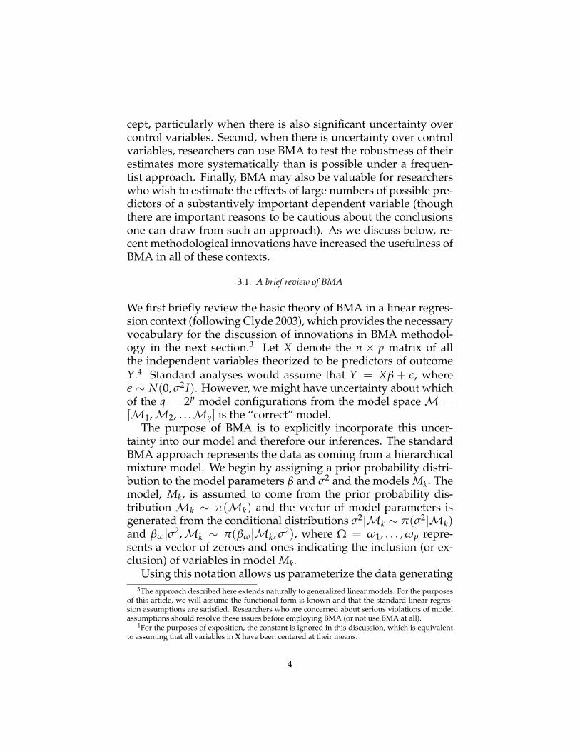
Rather than relying on summary statistics, the best way to un-derstand the properties of posterior distributions is to plot themfor each parameter, which is now trivial with publicly availablesoftware. Figure 1 illustrates what a coefficient posterior plotlooks like. These plots allow us to answer two distinct questions:
1. Does the variable contribute to the model’s explanatory power?(i.e. what is the posterior probability of all models that in-clude this variable?)
2. Is it correlated with unexplained variance when it is included?(i.e. what is the conditional posterior distribution assumingthat the variable is included?)
[Figure 1 about here.]
The vertical line located at 0 on the x-axis represents the cumu-lative posterior probability of all models that exclude the relevantvariable. One minus this value is the posterior probability of in-clusion, p(βk 6= 0|Y), which can be used to answer question 1above. The conditional posterior distribution, which is also in-cluded in the plot, represents the estimated value of the coefficientin the models in which it is included weighted by the likelihoodof those models, p(β|β 6= 0, Y). The location and density of thisdistribution allows us to answer question 2 above.
7
A related point is that BMA encourages researchers to be moreclear about their statistical hypotheses. In practice, many scholarsmay wish to distinguish between the conditional posterior distri-bution and the posterior probability of inclusion depending ontheir goals and the nature of the data. For instance, some schol-ars are primarily interested in whether an independent variableis strongly correlated with a dependent variable across a rangeof potential model configurations. In such cases, BMA allows re-searchers to calculate p(β > 0|β 6= 0, Y) or p(β < 0|β 6= 0, Y)for the conditional posterior distribution, an option that we haveadded to the BMA and BAS packages. Alternatively, a scholarwho is more interested in prediction (say, a scholar of interstatewar) may want to know whether a predictor adds to the explana-tory power of statistical models for a given dependent variable(or whether it offers more explanatory power than some alternateconcept). In this context, it might be appropriate to focus on theposterior probability of inclusion. Finally, other researchers maywish to consider both metrics and use the combined posterior dis-tribution p(β|Y).7
4.2. Searching the full model space
A second major difference in our approach is that that we adviseresearchers to consider the full set of 2p possible models whenconducting model averaging (excluding those that are theoret-ically or statistically inappropriate, as described below). Someearly presentations of BMA focused on averaging across very smallsubsets of the model space. For instance, in the two examples hepresents, Bartels limits his model averaging to a handful of modelspecifications reported in published work, which implicitly placesa zero prior on all other possible models. He concedes that his ap-proach “can provide only a rough reflection of real specificationuncertainty” but argues that it reflects the “substantive insight”of researchers (1997, 667-670).
However, putting a non-zero prior probability on only a hand-7Current practices in the discipline rely heavily on p values, which awkwardly conflate these
two concepts (Gill 1999). Separating them allows for useful distinctions in variable performance.For instance, it is possible to have variables that are “statistically significant” (i.e., their credibleintervals do not overlap with zero) but have low posterior probabilities of inclusion. Likewise, itis possible for a variable with a high posterior probability of inclusion to have a model-averagedcredible interval that overlaps with zero due to variation in sign and significance across models.
8

ful of models when using BMA is almost always a mistake. Sub-stantively, it typically will overstate our certainty that the includedmodels are the only possible choices. In addition, such restric-tions cripple the greatest strength of BMA—its ability to system-atically search a model space and present posterior estimates thatincorporate uncertainty in the model specification. Even Erik-son, Wright and McIver (1997)—the authors of one of the arti-cles whose models were reanalyzed—dissent, noting that “theoriginal model averaging literature is unambiguously clear in itsrule that all models involving plausible variables must be consid-ered.”8 Previously, researchers might have been forced to restrictthe model space due to computational limitations, but the inno-vations in BMA software discussed above have made it possibleto analyze large numbers of covariates.
4.3. Alternative prior specifications to BIC
In addition, most early BMA research, including Bartels (1997),approximated Bayes factors using the Bayesian Information Cri-terion (Raftery 1995, 129-133).9 While this approach was com-putationally convenient, its consequences were not always desir-able. For instance, BIC tends to place a relatively high posteriorprobability on sparse models (Kass and Raftery 1995; Kuha 2004;Erikson, Wright and McIver 1997), a model prior that is not al-ways substantively appropriate. In addition, though advocates ofBIC argue that it is a reasonable approximation of the Bayes fac-tor under a unit information prior (Raftery 1995, 129-133), Gelmanand Rubin (1995) note that BIC does not correspond to a properBayesian prior distribution (see also Weakliem 1999).
However, other prior specifications are now available to ap-plied researchers. In conjunction with advances in techniquesfor sampling large model spaces, these new priors have allowedresearchers to significantly improve the flexibility and power ofBMA techniques while avoiding shortcuts such as BIC and AIC.10
8Searching such a limited model space may also lead to an unwarranted emphasis on the selec-tion of the “best” model, which is generally of limited substantive interest.
9The BIC for model Mk compared to the null model M0 is BICk = −2 log(Lk − L0) + p log nwhere Lk is the maximized likelihood for Mk and p is the number of parameters in the model.
10While BIC and AIC are not proper Bayesian priors (Gelman and Rubin 1995), we will some-times refer to them as “priors” for expositional clarity.
9
One option in the BAS package that has appealing propertiesis Zellner’s g-prior (Zellner 1986), which is formulated as
π(βω|Mk, σ2) ∼ Npω(0, gσ2(X′ωXω)−1) (4)
andπ(β0, σ2|Mk) ∝ 1/σ2 (5)
for some positive constant g where pω represents the number ofpredictor variables in the ωth model.11 It yields closed form ex-pressions for p(Y|Mk) that are rapidly calculable and requires thechoice of only one hyperparameter, simplifying the prior specifi-cation process. However, this approach requires the analyst toselect a value of g12, which may lead to possible misspecification.
Alternatively, one can place a hyper-prior on g. Here we in-troduce two such hyper-priors for linear regression, which areanalyzed in Liang et al. (2008) and available for use in the BASpackage. The first, the so-called “hyper-g,” puts the followinghyper-prior on g:
π(g) =a− 2
2(1 + g)
a2 for g > 0. (6)
Liang et al. (2008) use example values of 3 or 4 for a when specify-ing the hyper-g but state that values of 2 < a ≤ 4 are “reasonable”(the distribution is proper when a > 2). A related approach is theZellner-Siow prior (Zellner and Siow 1980). To create this prior,we put a Gamma(1/2, n/2) prior on g, which induces a multi-variate Cauchy prior on βω:
π(βω|Mω, σ2) ∝∫
N(βω|0, gσ2(X′ωXω)−1)π(g) dg. (7)
Both priors have desirable asymptotic properties and perform wellin simulations (Liang et al. 2008).
How should one choose among the various prior options thatare now available? As noted above, BIC tends to favor parsimo-nious models, while AIC tends to include more parameters (Kassand Raftery 1995; Kuha 2004). The hyper-g, and Zellner-Siow pri-ors will tend to fall somewhere in between. In practice, one’s
11All variables are assumed to be centered at zero in this notation.12In particular, one can often choose a value for g that corresponds to the AIC and BIC approxi-
mations, although this value may not necessarily be known.
10
choice should depend on the goals of the research project, the na-ture of the data, and the type of model. However, the method weadvocate—and which we use in our examples below—is to an-alyze data with respect to multiple priors in order to assess thesensitivity of one’s results to prior choice.
4.4. Specifying model priors
A related development in BMA methodology involves specify-ing more flexible priors over models. Per Clyde (2003) and Clydeand George (2004), we can think of placing a prior distribution onmodelsM1 . . .Mk by treating the indicator variables ω as result-ing from independent Bernoulli distributions
π(Mk) = γpω(1− γ)p−pω . (8)
This prior is fully specified by the selection of the hyperparameterγ ∈ (0, 1), which can be thought of as the probability that eachpredictor variable is included in the model.
The vast majority of previous presentations have assumed auniform distribution over models.13 This assumption implies thatγ = .5 and that the number of parameters is distributed binomial(q, .5) over the q = 2p models, which means that the expectednumber of independent variables in a model is p/2 (Clyde 2003).
However, the assumption of a uniform distribution over mod-els is not always appropriate (Erikson, Wright and McIver 1997).The BAS package offers several options for specifying priors overmodels that reflect researchers’ understanding of the data gen-erating process. First, analysts can select a value for γ that cor-responds to their prior beliefs about the appropriate number ofpredictors in the model. Analysts with prior beliefs about theinclusion of specific variables can also represent γ as a vectorγ = (γ1, γ2, ..., γp), where γi represents the prior probability thatvariable i should be included in the model. Finally, a third pos-sible approach is to put a beta prior on the hyperparameter γ toreflect the range of complexity we expect in the posterior modelspace.
13Bartels does so as well in his main analysis (1997, 669). (He also introduces “dummy-resistant”and “search-resistant” priors, but these have not come into wide usage and we therefore do notdiscuss them further.)
11
4.5. Properly handling interaction terms
Finally, it is necessary to adjust BMA usage to account for thepresence of interaction terms, which are frequently employed insocial science data analysis. In his analysis, Bartels averages overmodels that vary in whether they include one or more interactionterms derived from variables of theoretical interest. However, thecoefficient for a constitutive term of an interaction represents themarginal effect of that variable when the other constitutive termis equal to zero (Braumoeller 2004; Brambor, Clark and Golder2006). Combining coefficient estimates of constitutive terms withestimates of the same coefficients from models that omit the in-teraction creates an uninterpretable mixture of estimates of twodifferent quantities.14
We recommend a different approach that is consistent withcontemporary statistical practice. First, if an interaction term isone of the covariates under consideration, we should avoid aver-aging over models in which one or more of its constitutive termsare excluded (Braumoeller 2004; Brambor, Clark and Golder 2006).To do otherwise assumes that the marginal effect of the excludedvariable is zero. If this assumption is false, the interaction termwill be incorrectly estimated. In addition, if an interaction termand its constitutive terms are quantities of theoretical interest (ratherthan control variables), it is desirable to average within the subsetof models that include the constitutive terms and the interactionterm. The resulting posterior distributions for the interaction andthe constitutive terms will then have consistent conceptual defi-nitions and can be interpreted properly.
Previously, it was impossible for the applied analyst to restrictthe set of analyzed models in this way without writing new code.For instance, Erikson, Wright and McIver (1997) express concernthat BMA “does not seem adaptable to models containing mutu-ally exclusive dummy variables or complicated interaction terms.”
14For instance, the coefficients for state opinion and Democratic legislative strength in the Erik-son, Wright and McIver data that Bartels reanalyzes represent the marginal effect of those vari-ables in “individualistic” states when interactions with state political culture indicators from Elazar(1972) are included (i.e. “individualistic” is the reference category and is therefore excluded). Bycontrast, when the interaction terms are omitted from the model, the coefficients for state opinionand Democratic legislative strength represent their unconditional marginal effects. A similar cri-tique applies to Bartels’s other example, which reanalyzes models of economic growth in OECDcountries by Lange and Garrett (1985) and Jackman (1987).
12
To address this concern, we have modified the BMA and BASpackages to allow analysts to easily exclude theoretically inappro-priate models from the averaging process. Using these softwareoptions, analysts can drop models that violate important theoret-ical or statistical assumptions. For instance, it is possible to dropall models in which an interaction term or its constitutive vari-ables are excluded as described above.
5. APPLYING BMA: THREE ILLUSTRATIVE EXAMPLES
In this section, we present three examples of how BMA can be ap-plied in contemporary political science research using the method-ological approach described above. Our first example examinesthe Adams, Bishin and Dow (2004) study of voting in U.S. Sen-ate elections, illustrating how BMA can be used to arbitrate be-tween two possible measures of the same concept (voter utilityfrom candidate positioning in one dimension). Second, we reana-lyze the Canes-Wrone, Brady and Cogan (2002) study of the effectof roll-call extremity on incumbent support in the U.S. House ofRepresentatives, which illustrates how BMA can be used to testthe robustness of a single predictor against a wide array of al-ternative specifications including interactions. Our final exampleillustrates how BMA can help validate the robustness of one’s sta-tistical results in a vast model space using data from Fearon andLaitin’s (2003) analysis of the onset of civil war.
5.1. U.S. Senate voting
We begin with an example that demonstrates how the BMA ap-proach can help arbitrate between competing predictors. Adams,Bishin, and Dow (henceforth ABD) use data from the 1988-1990-1992 Pooled Senate Election Study to “evaluate the discounting/ directional hypothesis versus the alternative proximity hypoth-esis” (348). Using both an individual-level model of vote choiceand an aggregate-level model of vote share, they “find a consis-tent role” for their directional variables, while results for theirproximity variables are weaker and less consistent (368). We fo-cus here only on their aggregate-level results (see Montgomeryand Nyhan 2008 for a reanalysis of their individual-level results).
13
ABD follow the common approach of putting alternative mea-sures into the same model and basing their inferences on the re-sulting coefficients—a practice that Achen (2005) refers to as a“pseudo-theorem” of political science. Unfortunately, as Achenshows, this practice is likely to lead to incorrect inferences. A bet-ter approach is to use BMA, which allows us to test competingmeasures in a more coherent fashion.15
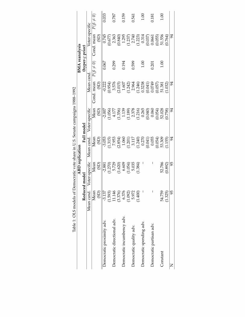
ABD conduct an OLS analysis in which they predict the per-centage of the two-party vote received by the Democrat in eachelection. They focus on two independent variables of interest,which they call Democratic directional advantage and Democraticproximity advantage, and estimate two types of models—one inwhich these variables are calculated using the average ideolog-ical placement of that candidate by all respondents in the rele-vant state and year (which we will refer to as “mean candidateplacement”) and one in which the variables are calculated usingrespondents’ own placements of the two candidates (which wewill refer to as “voter-specific placement”).16 These four differ-ent measures are then aggregated at the campaign level. In addi-tion, ABD express some uncertainty about the correct set of con-trol variables to include in the analysis, resulting in the reportingof two models for each variable of interest.
Columns 1–4 of Table 1 present our replication of ABD’s Ta-ble 2, which incorporates corrections of several errors in the pub-lished results (see the appendix for a more extensive discussionof our replication). The corrected results, which serve as the ba-sis for the BMA analysis below, show that the directional vari-able is consistently positive and statistically significant but thatthe proximity variable is consistently negative and significant.17
This result contradicts spatial voting theory, which suggests that15Some studies have argued for combining directional and spatial approaches (e.g. Iversen 1994;
Adams and Merrill 1999; Merrill and Grofman 1999). However, we interpret the ABD paper as anattempt to arbitrate between directional/discounting and proximity models.
16For the voter-specific evaluation, the proximity score is created by using the formula [(xR −xi)2 − (xD − xi)2], where xR and xD are the respondent’s placements of the Republican and Demo-cratic candidates (respectively) on a seven-point Likert scale of ideology and xi is the respondent’sself-placement on that scale. For the voter-specific evaluation of the directional score, the relevantequation is [(xD− 4)(xi − 4)− (xD− 4)(xi − 4)]. The mean candidate variables are identical exceptthat the average placements of each candidate from all respondents in that state and year are usedfor xR and xD.
17In the published version of the table, the proximity variable is insignificant and changes signsacross specifications (see appendix).
14
a party’s ideological proximity to voters should be positively as-sociated with its share of the vote. Moreover, the magnitude of thedirectional coefficients raise concerns about misspecification. Forinstance, the results in the first column of Table 1 indicate that aone unit increase in the Democratic directional advantage (a vari-able with a range that exceeds 4 in the data) results in a 11% in-crease in the Democratic share of the two-party vote.
[Table 1 about here.]
As stated earlier, it is inappropriate to include two competing(and highly correlated) measures of a concept in the same model.Our BMA analysis therefore considers the entire model space im-plied by the five variables in the original model excluding thosemodels containing both the directional and proximity variables.18
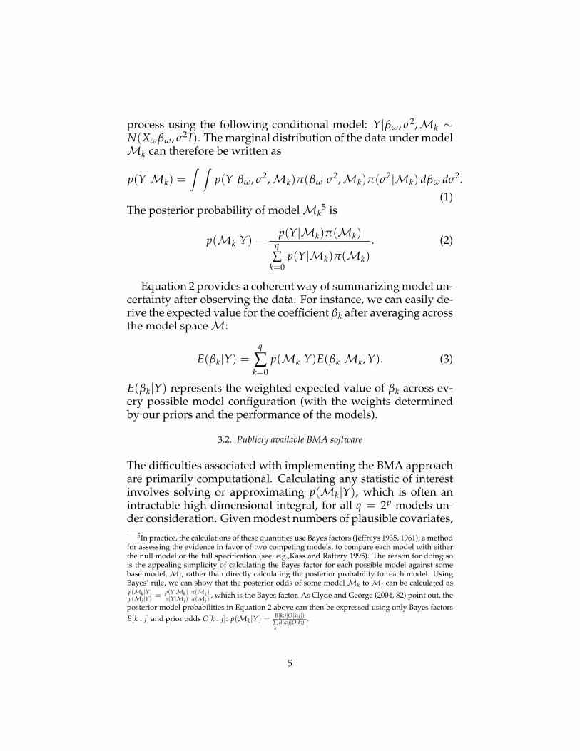
Because the dependent variable is continuous, we can use theBAS package. Columns 5–8 report our findings for the hyper-gprior (a=3) with a uniform prior on the model space. Results weresubstantively identical under AIC, BIC, and Zellner-Siow, as illus-trated by Figure 2, which presents posterior plots for the variablesof theoretical interest under all four priors.
[Figure 2 about here.]
We focus on the posterior probability of inclusion as the bestmetric for arbitrating between two possible measures of the sameconcept. In this case, our findings show considerably less supportfor ABD’s conclusions than our replication of their original tables.The posterior probability of inclusion for the directional measuresis consistently higher than the proximity variables. However, theDemocratic directional advantage variable in the “mean candi-date placement” model has a posterior probability of inclusion ofonly 0.30, which suggests that the variable is a relatively weakpredictor of electoral outcomes.
The results reported in columns 5–8 suggest that the negativecoefficient on the proximity variables and the large coefficientsassociated with the directional measures were artifacts of includ-ing both measures in the same regressions. When we exclude
18In the text, ABD identify variables that were considered but not included in the final analysis.For expositional purposes, we do not consider them there. We demonstrate the utility of BMA forreanalyzing alternate control variables in our reanalysis of Fearon and Laitin (2003b) below.
15
models that include both variables and average across the remain-ing model space, we find that the proximity variable has a min-imal rather than a negative coefficient. Second, the size of thecoefficients for the directional variables are substantially reduced.These findings illustrate the inferential dangers of including com-peting measures of a single concept in a statistical model, anddemonstrate how BMA can help arbitrate between such measuresin a systematic way.
5.2. U.S. House elections
In their widely-cited 2002 article, Canes-Wrone, Brady, and Co-gan (henceforth CWBC) combine summary measures of roll-callvoting with electoral returns to show that legislative extremity re-duces support for members of the U.S. House of Representativesin future elections. Their work demonstrates an important link-age between Congressional behavior and electoral outcomes. Italso provides a classic example of a research design intended todemonstrate the robustness of the relationship between a singlepredictor and a dependent variable.
The focus of the CWBC analysis is their measure of roll-callideological extremity, which is based on ratings of House mem-bers provided by Americans for Democratic Action (ADA).19 Forexpositional reasons, we focus here only on the full version oftheir pooled model (column 2 of Table 2 in their article), whichestimates the effect of extremity on a member’s share of the totaltwo-party vote for the 1956–1996 period.
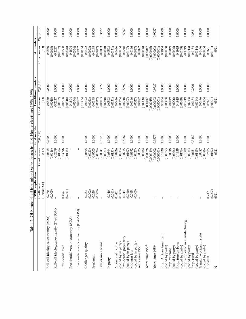
The pooled model that CWBC present, which is replicated inthe first column of Table 2 below, includes a measure of the dis-trict presidential vote (which is intended to serve as a proxy forparty strength in the district) and seven other control variables.These controls are presumably included to help ensure that anyrelationship they find is not spurious. However, we can use BMAto assess the robustness of their model across a wider range ofplausible control variables. The literature on US elections sug-gests a number of other possible factors that might also be asso-ciated with electoral vote share. In this reanalysis, we consider
19It is calculated as the ADA score for Democratic members and 100 minus the ADA score forRepublican members so that higher values represent greater extremity by party (Canes-Wrone,Brady and Cogan 2002, 131). The resulting score is then divided by 100.
16
variables measuring the demographic characteristics of the dis-trict (the proportion of district residents who live in rural settings,the proportion who work in the manufacturing sector, and theproportion who are African Americans, union members, foreignborn, or veterans)20, incumbency (an indicator for members whohave served five or more terms), and a flexible function of yearssince 1956 (i.e. linear, squared, and cubed terms) to capture thechanging magnitude of the incumbency advantage in this period.
We also use BMA to consider an alternate measure and a pos-sible moderator. CWBC note (but do not show) that their re-sults hold using an average of first and second dimension DW-NOMINATE scores (Poole and Rosenthal 1997, 2007) instead ofADA ratings. Since the average score across two dimensions isdifficult to interpret, we instead transform DW-NOMINATE first-dimension scores by party (following the CWBC ADA measure)to assess how results compare between two possible measuresof roll call extremity.21 Finally, it is plausible that the electoralpunishment for extremity may vary depending on the partisancomposition of the district. As such, we separately interact bothmeasures of roll-call extremity with the CWBC measure of districtpresidential vote to assess whether the strength of the relationshipis conditional on party strength in the district.
In each case, we also exclude all models that include compet-ing measures of the same concept (i.e. those that include one ormore ADA-based variables and one or more DW-NOMINATE-based variables), those that do not include a dummy variable forbeing in the incumbent president’s party (it implicitly interactswith several other variables of interest), and all models that in-clude the cubed or squared term for years since 1956 but excludea lower-order polynomial. Following our recommendations foranalyzing interactions (described above), we analyze the uncon-ditional effect of roll-call extremity and the conditional effect inseparate models before pooling terms to assess the posterior prob-ability of inclusion for the interaction terms.
Table 2 provides model outputs from the BMA analysis usinga Zellner-Siow prior on the coefficients and a Beta (3,2) prior on
20These variables are drawn from Adler (forthcoming). In each case, the values are multipliedby -1 for Republicans to allow for differing effects by party.
21Specifically, we multiply Democrats’ first dimension scores by -1 and then rescale the resultingvariable to range from 0 to 1.
17
the model hyperparameter γ.22
[Table 2 about here.]
As noted above, the table contains three models. The first, whichis reported in columns 2–3, considers the unconditional effect ofextremity and therefore excludes all models with interaction terms.This analysis allows us to estimate the robustness of the CWBCfinding across a large model space. The second model, whichis reported in columns 4–5, examines the potential moderatingeffects of district party strength and therefore excludes all mod-els that do not include a properly specified interaction with bothconstitutive terms. In this case, we can interpret the posteriordistributions of the extremity constitutive term and interactionas we would in a normal interaction model.23 Finally, the thirdmodel, which is reported in columns 6–7, includes the interactionterms in the averaging process but does not require them to be in-cluded (though we again omit all models with an interaction thatomit one or more constitutive terms). The resulting estimates forthe constitutive terms are not necessarily interpretable, but thismodel allows us to use the posterior probability of inclusion toassess the importance of the interaction terms.
Comparing these results with those reported in the originalstudy (column 1) leads us to three conclusions.24 First, the un-conditional effect of extremity on electoral support, as shown incolumns 2–3, is robust to a large set of possible model configura-tions. The CWBC hypothesis is supported across a vast space ofmore than 98,000 models.
Second, we find that measures of roll-call extremity constructedusing DW-NOMINATE scores perform substantially better in allcircumstances than those created using ADA scores. The DW-NOMINATE extremity variable dominates the posterior space inall the analyses with a posterior probability of inclusion approach-
22The posterior probability plots for the main coefficients of interest are not shown for exposi-tional reasons but are available upon request. In this case, they are regularly shaped and provideno additional information beyond the posterior summary statistics provided in Table 2.
23Note that we cannot interpret the constitutive term for district presidential vote as we wouldnormally would (the marginal effect when the extremity variable equals zero) since it is interactedwith two different measures of roll-call extremity.
24The substantive inferences discussed below are consistent across multiple priors (results avail-able upon request). The original CWBC analysis used robust standard errors, which are not avail-able in BMA and thus not included in the analysis below.
18
ing one. By contrast, the ADA extremity variable and its associ-ated interaction term have extremely low posterior probabilitiesof inclusion. For instance, the posterior probabilty of inclusionfor the ADA-based extremity measure in the unconditional modelreported in columns 2–3 is 5.930× 10⁻⁶.
Third, the effect of roll-call extremity on election results is mod-erated by party strength in the district (as measured by the CWBCpresidential vote variable). The DW-NOMINATE interaction termis highly statistically significant in columns 4–5 (p(β > 0| β 6=0, Y) > .999) and its posterior probability of inclusion in the pooledmodel in columns 6–7 is approximately one. Substantively, theseresults indicate that members from very marginal districts suf-fer severe punishment for legislative extremity but the electoralcost of extremity declines rapidly as party strength in the districtincreases. In those districts in which the party is strongest, themarginal effect of roll-call extremity is actually either negligible(i.e. the 95% confidence interval includes zero) or positive.25 Inother words, members are punished to the extent they are out ofstep with their district.26
5.3. Civil war onset
In a groundbreaking study, Fearon and Laitin (2003b) seek to de-termine the most important predictors of civil war onset (a binarydependent variable). Their reported logit models estimate the ef-fects of thirteen explanatory variables. However, throughout thetext, footnotes, and additional results posted online (2003a), F&Lare unusually transparent in describing numerous other variablesand interactions that were considered during the modeling pro-cess. In short, they acknowledge a great deal of uncertainty aboutthe final model configuration that cannot be analyzed using tradi-tional methods. Indeed, the length of their online supplement—which is 30 pages and contains 18 multi-column tables—indicates
25To fully understand this effect, it was necessary to estimate the marginal effect of extremityover the observed range of district presidential vote in a single model (Brambor, Clark and Golder2006). We selected the model containing the interaction and its constitutive terms with the highestposterior probability (.24). Since the sign and significance of the interaction and its constitutiveterms were consistent with the conditional posterior distributions in the BMA analysis, the re-sulting marginal effect estimates should be representative of the set of models that include theinteraction. All results of this analysis are available upon request.
26Griffin and Newman (2009) find a similar result using data from the 2000 and 2004 NationalAnnenberg Election Study.
19
the need for a more concise approach to specification uncertainty.Fearon and Laitin’s transparency allows us to identify a num-
ber of other variables that were considered to be plausible pre-dictors of civil war onset. We estimate that F&L discuss approx-imately 74 possible independent variables (excluding various in-terpolation/missing data decisions), which implies a potential spaceof roughly 2 × 10²² potential models. As noted earlier, the tra-ditional approach does not allow researchers to properly expressuncertainty about their estimates when faced with such vast modelspaces. For instance, consider the following quote (2003b, 84):
When we add dummy variables for countries that havean ethnic or religious majority and a minority of at least8% of the country’s poulation, both are incorrectly signedand neither comes close to statistical significance. Thisfinding does not depend on which other variables are includedin the model (emphasis ours).
Obviously, F&L did not test these variables under all 20 sextil-lion possible specifications. One suspects that they tried addingrelevant variables to their “best” models and found they were in-significant (one such model is reported in Table 3 of Fearon andLaitin 2003a).27 BMA makes it possible to systematically justifysuch statements.
In this analysis, we chose a subset of F&L’s variables to eval-uate. One of the limits of BMA is that the model space q = 2p
can quickly exceed the abilities of even the most advanced com-puters to fully explore the posterior model distribution. Clyde(2003) recommends that any models that use more than approxi-mately 25 variables should be analyzed using stochastic samplingtechniques rather than deterministic search algorithms. However,no publicly available BMA software performs stochastic samplingfor GLM models (but see Pang and Gill 2009). As such, we chose25 publicly available variables that had no missing data in thesame universe of cases that F&L analyze, which allows us to ex-plore the entire posterior distribution using the bic.glm functionin the BMA package. To reduce the software limitations describedabove, we effectively disable the model selection criterion, ensur-ing that the software returns the maximum number of relevant
27This should not be interpreted as a criticism of Fearon and Laitin’s important article. Manystudies, including ones we have participated in, use this approach.
20
models, and create an option to use the Akaike Information Cri-terion (AIC) instead of BIC (Akaike 1974).
Per our earlier discussion, we also place theoretically moti-vated limitations on the models we wish to explore. Specifically,we put a zero prior on all models that do not contain the key ex-planatory variable indicating the existence of a prior war. We alsoput a zero prior on models that contain both the Polity IV measureof democracy and dummy variables for democracy and anocracyderived from Polity IV or include only one of the anocracy anddemocracy dummy variables. In each case, we seek to adhere tostandard procedures in the political science literature.
We replicate their primary models of civil war onset in columns1 and 2 of Table 3.28
[Table 3 about here.]
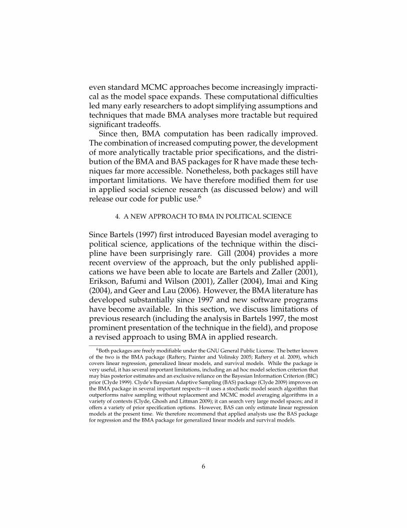
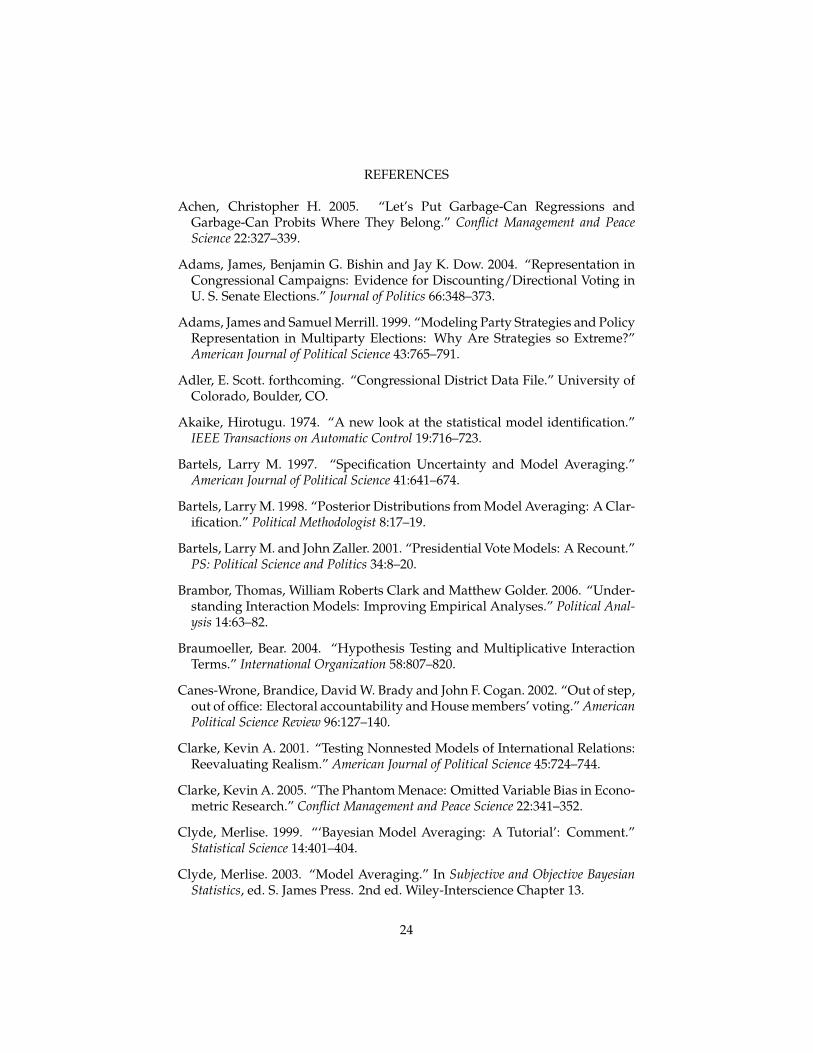
Columns 3–6 of Table 3 provide conditional means, standard de-viations, and posterior probabilities of inclusion under AIC andBIC.29 Posterior plots under AIC are presented in Figure 3.30
[Figure 3 about here.]
Although the table and figure contain a great deal of informa-tion, we highlight two key findings. First, conditional posteriordistributions for the variables that F&L identify as statisticallysignificant predictors of civil war onset—prior war, per capitaincome, log(population), log(% mountainous), oil exporter, newstate, instability, and anocracy— are consistent with their originalresults. BMA therefore provides a truly systematic demonstrationof the robustness of F&L’s results (and does not require 30 pagesof tables to do so!). However, most of F&L’s predictors (whichare frequently measured imprecisely) have low posterior proba-bilities of inclusion under BIC (column 6). Besides the constantand the prior war variable (which we required to be included in
28These models correspond to Models 1 and 3 in F&L. We do not address the three other modelsthey report, which use different dependent variables.
29Before performing our analysis, we dropped a single observation with a miscoded value forthe dependent variable from F&L’s data. In order to assure that enough models were sampled, weset the leaps and bounds algorithm employed by bic.glm to return the 100,000 best models for eachpossible rank of X.
30It’s worth noting that the BMA package assumes that the posterior distribution of each coeffi-cient is normal, while BAS assumes they are distributed Student t with one degree of freedom. Asa result, BMA plots tend to be more smooth than those generated by BAS.
21
each model), only per-capita income, logged population, and theindicator of a new state have a posterior probability of inclusionof more than 0.5—a result that underscores the need to examinethe sensitivity of one’s results to priors.
6. CAUTIONS AND CONCLUSIONS
Political science researchers are often confronted with substantialuncertainty about the robustness of reported results. In manyprominent literatures, researchers have proposed dozens (if nothundreds) of potential explanatory variables. Classical approachesto modeling techniques provide researchers with few tools fordealing with this uncertainty. As a result, readers are frequentlyconcerned about alternative model configurations that were triedbut not reported — and those that were never tried at all.
BMA offers researchers a comprehensive method for assessingmodel uncertainty that can easily be presented to readers. In thispaper, we have reviewed recent developments in prior specifica-tions and posterior computation techniques, presented a contem-porary approach to the use of BMA, and applied this methodol-ogy to three prominent studies from the discipline. Our empiricalanalyses revealed substantive differences in the effects of the the-oretical variables of interest from Adams, Bishin and Dow (2004),demonstrated the conditional nature of the main effect reportedin Canes-Wrone, Brady and Cogan (2002), and gave a more rig-orous foundation to the findings presented in Fearon and Laitin(2003b). In general, we strongly believe that BMA can strengthenthe robustness of reported results in political science.
Despite the usefulness of the technique, we wish to concludewith words of caution about the appropriate use of BMA. First,we emphasize that it should not be used to conduct theory-freesearches of the model space, particularly if such a step is not re-ported to readers. BMA also offers no solutions to the problemsof endogeneity or causal inference. Statistical analysis should be-gin with the careful development of a model based on theory andprevious research (Gelman and Rubin 1995). BMA is best used asa subsequent robustness check to show that our inferences are notoverly sensitive to plausible variations in model specification.
On a related note, we also caution that BMA—like all statisti-
22
cal methods—cannot defeat unscrupulous researchers. While itshould be more difficult to manipulate BMA analysis than, say, asingle reported model specification, researchers could alter the setof variables that are averaged to try to support a desired finding.Similarly, one could use BMA to identify a model specificationthat maximizes fit to the data and then present that choice as theresult of theory. As in all such cases, we must trust in the good in-tentions of the researcher and use theory to guide our judgmentsabout the set of independent variables that should be considered.
With those caveats in mind, we hope that more analysts makeuse of BMA, which makes it possible to systematically test therobustness of our findings to a much wider array of model speci-fications than is otherwise possible.
23
REFERENCES
Achen, Christopher H. 2005. “Let’s Put Garbage-Can Regressions andGarbage-Can Probits Where They Belong.” Conflict Management and PeaceScience 22:327–339.
Adams, James, Benjamin G. Bishin and Jay K. Dow. 2004. “Representation inCongressional Campaigns: Evidence for Discounting/Directional Voting inU. S. Senate Elections.” Journal of Politics 66:348–373.
Adams, James and Samuel Merrill. 1999. “Modeling Party Strategies and PolicyRepresentation in Multiparty Elections: Why Are Strategies so Extreme?”American Journal of Political Science 43:765–791.
Adler, E. Scott. forthcoming. “Congressional District Data File.” University ofColorado, Boulder, CO.
Akaike, Hirotugu. 1974. “A new look at the statistical model identification.”IEEE Transactions on Automatic Control 19:716–723.
Bartels, Larry M. 1997. “Specification Uncertainty and Model Averaging.”American Journal of Political Science 41:641–674.
Bartels, Larry M. 1998. “Posterior Distributions from Model Averaging: A Clar-ification.” Political Methodologist 8:17–19.
Bartels, Larry M. and John Zaller. 2001. “Presidential Vote Models: A Recount.”PS: Political Science and Politics 34:8–20.
Brambor, Thomas, William Roberts Clark and Matthew Golder. 2006. “Under-standing Interaction Models: Improving Empirical Analyses.” Political Anal-ysis 14:63–82.
Braumoeller, Bear. 2004. “Hypothesis Testing and Multiplicative InteractionTerms.” International Organization 58:807–820.
Canes-Wrone, Brandice, David W. Brady and John F. Cogan. 2002. “Out of step,out of office: Electoral accountability and House members’ voting.” AmericanPolitical Science Review 96:127–140.
Clarke, Kevin A. 2001. “Testing Nonnested Models of International Relations:Reevaluating Realism.” American Journal of Political Science 45:724–744.
Clarke, Kevin A. 2005. “The Phantom Menace: Omitted Variable Bias in Econo-metric Research.” Conflict Management and Peace Science 22:341–352.
Clyde, Merlise. 1999. “‘Bayesian Model Averaging: A Tutorial’: Comment.”Statistical Science 14:401–404.
Clyde, Merlise. 2003. “Model Averaging.” In Subjective and Objective BayesianStatistics, ed. S. James Press. 2nd ed. Wiley-Interscience Chapter 13.
24
Clyde, Merlise and Edward I. George. 2004. “Model Uncertainty.” StatisticalScience 19:81–94.
Clyde, Merlise, Joyee Ghosh and Michael Littman. 2009. “Bayesian AdaptiveSampling for Variable Selection.” Unpublished manuscript.
Clyde, Merlise (with contributions from Michael Littman). 2009. BAS: BayesianModel Averaging using Bayesian Adaptive Sampling. R package version 0.45.URL: http://CRAN.R-project.org/package=BAS
Draper, David. 1995. “Assessment and Propagation of Model Uncertainty.”Journal of the Royal Statistical Society, Series B (Methodological) 57:45–97.
Elazar, Daniel J. 1972. American Federalism: A View from the States. 2nd ed. NewYork: Crowell.
Erikson, Robert S., Gerald C. Wright and John P. McIver. 1993. StatehouseDemocracy: Public Opinion and Policy in the American States. New York: Cam-bridge University Press.
Erikson, Robert S., Gerald C. Wright and John P. McIver. 1997. “Too ManyVariables? A Comment on Bartels’ Model-Averaging Proposal.” Presentedat the 1997 Political Methodology Conference, Columbus, Ohio.
Erikson, Robert S., Joseph Bafumi and Bret Wilson. 2001. “Was the 2000 Presi-dential Election Predictable?” PS: Political Science and Politics 34:815–819.
Fearon, James D. and David D. Laitin. 2003a. “Additional tables for ‘Ethnicity,Insurgency, and Civil War’.” Unpublished manuscript.
Fearon, James D. and David D. Laitin. 2003b. “Ethnicity, Insurgency, and CivilWar.” American Political Science Review 97:75–90.
Fernandez, Carmen, Eduardo Ley and Mark F. J. Steel. 2001. “Model uncer-tainty in cross-country growth regressions.” Journal of Applied Econometrics16:563–576.
Geer, John and Richard R. Lau. 2006. “Filling in the Blanks: A New Method forEstimating Campaign Effects.” British Journal of Political Science 36:269–290.
Gelman, Andrew and Donald B. Rubin. 1995. “Avoiding Model Selection inBayesian Social Research.” Sociological Methodology 25:165–173.
Gerber, Alan and Neil Malhotra. 2008. “Do Statistical Reporting StandardsAffect What Is Published? Publication Bias in Two Leading Political ScienceJournals.” Quarterly Journal of Political Science 3:313–326.
Gill, Jeff. 1999. “The Insignificance of Null Hypothesis Significance Testing.”Political Research Quarterly 52:647–674.
Gill, Jeff. 2004. “Introduction to the Special Issue.” Political Analysis 12:323–337.
25
Griffin, John and Brian Newman. 2009. “Assessing Accountability.” Paper pre-sented at the annual meeting of the Midwest Political Science Association.
Harrell, Frank E. 2001. Regression Modeling Strategies. Springer.
Ho, Daniel E., Kosuke Imai, Gary King and Elizabeth A. Stuart. 2007. “Match-ing as Nonparametric Preprocessing for Reducing Model Dependence inParametric Causal Inference.” Political Analysis 15:199–236.
Hoeting, Jennifer A., David Madigan, Adrian E. Raftery and Chris T. Volinsky.1999. “Bayesian Model Averaging: A Tutorial.” Statistical Science 14:382–401.
Imai, Kosuke and Gary King. 2004. “Did Illegal Overseas Absentee BallotsDecide the 2000 U.S. Presidential Election?” Perspectives on Politics 2:537–549.
Iversen, Torben. 1994. “Political Leadership and Representation in West Eu-ropean Democracies: A Test of Three Models of Voting.” American Journal ofPolitical Science 38:45–74.
Jackman, Robert W. 1987. “The Politics of Economic Growth in the IndustrialDemocracies, 1974-80: Leftist Strength or North Sea Oil?” The Journal of Poli-tics 49:242–256.
Jeffreys, Harold. 1935. “Some Tests of Significance, Treated by the Theory ofProbability.” Proceedings of the Cambridge Philosophical Society 31:203–222.
Jeffreys, Harold. 1961. Theory of Probability. 3rd ed. Oxford: Oxford UniversityPress.
Kass, Robert E. and Adrian E. Raftery. 1995. “Bayes Factors.” Journal of theAmerican Statistical Association 90:773–795.
King, Gary and Langche Zeng. 2006. “The dangers of extreme counterfactuals.”Political Analysis 14:131–159.
Kuha, Jouni. 2004. “AIC and BIC: Comparisons of Assumptions and Perfor-mance.” Sociological Methods Research 33.
Lange, Peter and Geoffrey Garrett. 1985. “The Politics of Growth: StrategicInteraction and Economic Performance in the Advanced Industrial Democ-racies, 1974-1980.” The Journal of Politics 47:792–827.
Liang, Feng, Rui Paulo, German Molina, Merlise A. Clyde and Jim O. Berger.2008. “Mixtures of g-priors for Bayesian Variable Selection.” Journal of theAmerican Statistical Association 103:410–423.
Madigan, David and Adrian E. Raftery. 1994. “Model Selection and Account-ing for Model Uncertainty in Graphical Models Using Occam’s Window.”Journal of the American Statistical Association 89:1535–1546.
26
Merrill, Samuel and Bernard Grofman. 1999. A Unified Theory of Voting: Direc-tional and Proximity Spatial Models. Cambridge University Press.
Montgomery, Jacob and Brendan Nyhan. 2008. “Bayesian Model Averaging:Theoretical developments and practical applications.” Society for PoliticalMethodology working paper.
Morales, Knashawn H., Joseph G. Ibrahim, Chien-Jen Chen and Louise M.Ryan. 2006. “Bayesian Model Averaging With Applications to BenchmarkDose Estimation for Arsenic in Drinking Water.” Journal of the American Sta-tistical Association 101:9–17.
Pang, Xun and Jeff Gill. 2009. “Spike and Slab Prior Distributions for Simul-taneous Bayesian Hypothesis Testing, Model Selection, and Prediction, ofNonlinear Outcomes.” Unpublished manuscript.
Poole, Keith T. and Howard Rosenthal. 1997. Congress: A political-economic his-tory of roll call voting. Oxford University Press, USA.
Poole, Keith T. and Howard Rosenthal. 2007. Ideology and Congress. TransactionPublishers.
Raftery, Adrian E. 1995. “Bayesian Model Selection in Social Research.” Socio-logical Methodology 25:111–163.
Raftery, Adrian E., Ian S. Painter and Christopher T. Volinsky. 2005. “BMA: AnR package for Bayesian Model Averaging.” R News 5:2–8.
Raftery, Adrian, Jennifer Hoeting, Chris Volinsky, Ian Painter and Ka Yee Ye-ung. 2009. BMA: Bayesian Model Averaging. R package version 3.12.URL: http://CRAN.R-project.org/package=BMA
Weakliem, David L. 1999. “A Critique of the Bayesian Information Criterionfor Model Selection.” Sociological Methods & Research 27:359–397.
Wintle, B.A., M.A. McCarthy, C.T. Volinsky and R.P. Kavanagh. 2003. “The Useof Bayesian Model Averaging to Better Represent Uncertainty in EcologicalModels.” Conservation Biology 17:1579–1590.
Yeung, Ka Yee, Roger E. Bumgarner and Adrian E. Raftery. 2005. “Bayesianmodel averaging: development of an improved multi-class, gene selectionand classification tool for microarray data.” Bioinformatics 21:2394–2402.
Zaller, John R. 2004. “Floating voters in U.S. presidential elections, 1948-2000.”In Studies in public opinion: Attitudes, nonattitudes, measurement error, andchange, ed. Willem Saris and Paul M. Sniderman. Princeton University Presspp. 166–214.
27
Zellner, Arnold. 1986. “On assessing prior distributions and Bayesian re-gression analyiis with g-prior distributions.” In Bayesian Inference and Deci-sion Techniques: Essays in honor of Burno de Finetti. North-Holland/Elsevierpp. 233–243.
Zellner, Arnold and Aloysius Siow. 1980. “Posterior Odds Ratios for SelectedHypotheses.” In Bayesian Statistics, ed. J. M. Bernardo, M. H. DeGroot, D. V.Lindley and A. F. M. Smith. Valencia, Spain: University Press.
28
APPENDIX: ADAMS, BISHIN, DOW (2004) REPLICATION
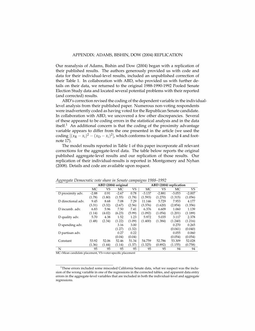
Our reanalysis of Adams, Bishin and Dow (2004) began with a replication oftheir published results. The authors generously provided us with code anddata for their individual-level results, included an unpublished correction oftheir Table 1. In collaboration with ABD, who provided us with further de-tails on their data, we returned to the original 1988-1990-1992 Pooled SenateElection Study data and located several potential problems with their reported(and corrected) results.
ABD’s correction revised the coding of the dependent variable in the individual-level analysis from their published paper. Numerous non-voting respondentswere inadvertently coded as having voted for the Republican Senate candidate.In collaboration with ABD, we uncovered a few other discrepancies. Severalof these appeared to be coding errors in the statistical analysis and in the dataitself.1 An additional concern is that the coding of the proximity advantagevariable appears to differ from the one presented in the article (we used thecoding [(xR − xi)2 − (xD − xi)2], which conforms to equation 3 and 4 and foot-note 17).
The model results reported in Table 1 of this paper incorporate all relevantcorrections for the aggregate-level data. The table below reports the originalpublished aggregate-level results and our replication of those results. Ourreplication of their individual-results is reported in Montgomery and Nyhan(2008). Details and code are available upon request.
Aggregate Democratic vote share in Senate campaigns 1988–1992ABD (2004) original ABD (2004) replication
MC VS MC VS MC VS MC VSD proximity adv. -2.88 0.91 -2.67 0.78 -3.137 -2.881 -3.053 -2.007
(1.78) (1.80) (1.55) (1.78) (1.593) (1.270) (1.315) (1.056)D directional adv. 9.45 8.68 7.08 7.29 11.146 5.729 7.953 4.177
(3.31) (3.32) (2.67) (2.56) (3.376) (1.620) (2.854) (1.356)D incumb. adv. 6.83 5.96 7.50 7.41 6.376 6.609 1.060 1.139
(1.14) (4.02) (6.23) (5.99) (1.092) (1.054) (1.201) (1.189)D quality adv. 5.70 4.38 1.52 1.23 5.972 5.035 3.117 2.378
(1.48) (2.34) (1.22) (1.09) (1.400) (1.384) (1.240) (1.216)D spending adv. 3.16 3.00 0.270 0.265
(1.27) (1.32) (0.041) (0.040)D partisan adv. 0.27 0.22 0.055 0.060
(0.04) (0.04) (0.054) (0.054)Constant 53.92 52.06 52.46 51.34 54.759 52.786 53.309 52.028
(1.36) (1.44) (1.14) (1.37) (1.325) (0.892) (1.155) (0.758)N 95 95 95 95 95 95 94 94
MC=Mean candidate placement, VS=voter-specific placement
1These errors included some miscoded California Senate data, what we suspect was the inclu-sion of the wrong variable in one of the regressions in the corrected tables, and apparent data entryerrors in the aggregate-level variables that are included in both the individual-level and aggregateregressions.
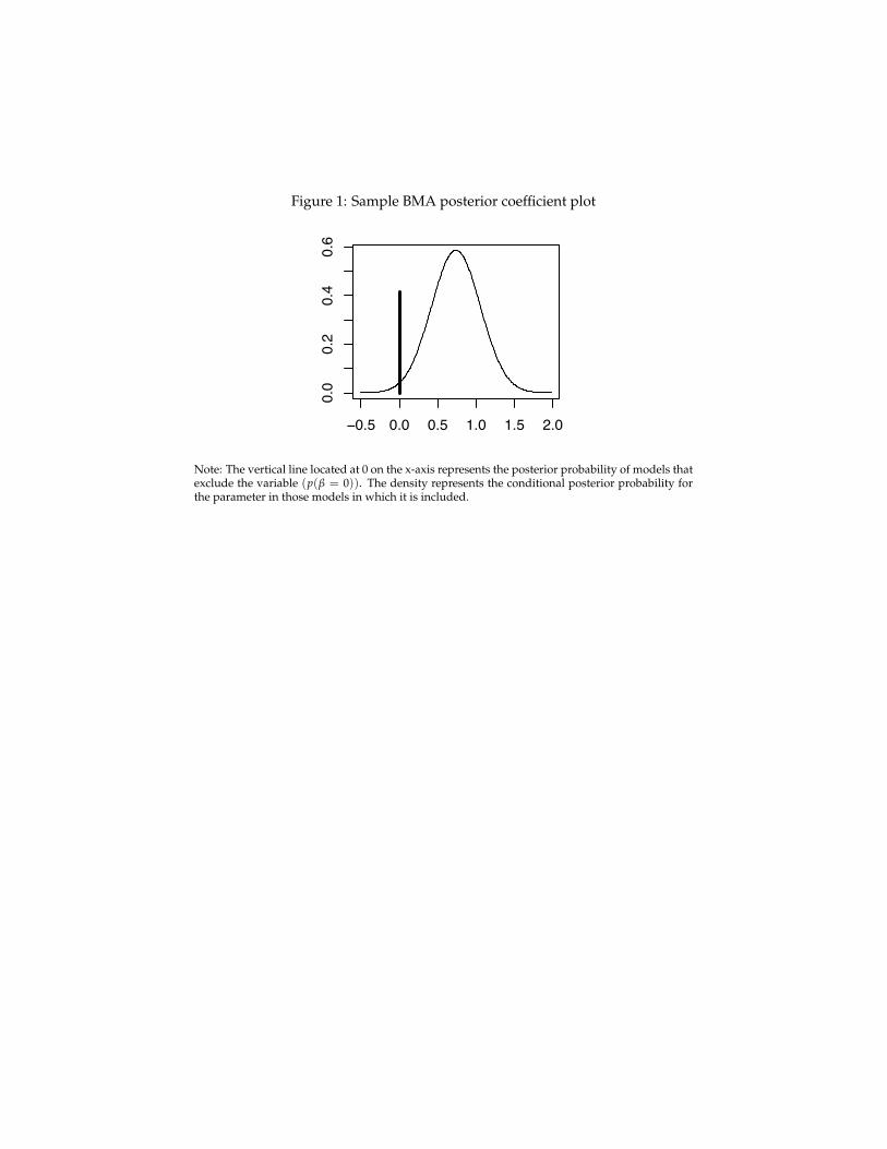
Figure 1: Sample BMA posterior coefficient plot
!0.5 0.0 0.5 1.0
0.0
0.4
0.8
Intercept
!0.5 0.0 0.5 1.0 1.5 2.0
0.0
0.2
0.4
0.6
x1
!1.5 !0.5 0.0 0.5
0.0
0.2
0.4
0.6
0.8
x2
!1.5 !0.5 0.5 1.0
0.0
0.4
0.8
x3
Note: The vertical line located at 0 on the x-axis represents the posterior probability of models thatexclude the variable (p(β = 0)). The density represents the conditional posterior probability forthe parameter in those models in which it is included.
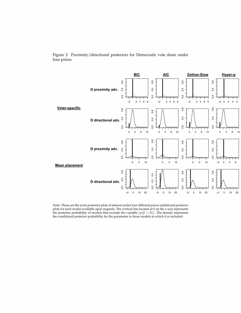
Figure 2: Proximity/directional posteriors for Democratic vote share underfour priors
!2 2 4 6 8
0.0
0.4
0.8
!2 2 4 6 8
0.0
0.4
0.8
!2 2 4 6 8
0.0
0.4
0.8
!2 0 2 4 6
0.0
0.4
0.8
0 4 8 12
0.0
0.4
0.8
0 4 8 12
0.0
0.4
0.8
0 4 8 12
0.0
0.4
0.8
0 4 8 12
0.0
0.4
0.8
0 5 10
0.0
0.4
0.8
0 5 10
0.0
0.4
0.8
0 5 10
0.0
0.4
0.8
!4 0 4 8
0.0
0.4
0.8
!5 5 15 25
0.0
0.3
0.6
!5 5 15 25
0.0
0.2
0.4
!5 5 15 25
0.0
0.3
0.6
!5 5 15 25
0.0
0.3
0.6
BIC AIC Zellner-Siow Hyper-g
D proximity adv.
Voter-specific
D directional adv. D proximity adv.
Mean placement
D directional adv.
Note: These are the main posterior plots of interest under four different priors (additional posteriorplots for each model available upon request). The vertical line located at 0 on the x-axis representsthe posterior probability of models that exclude the variable (p(β = 0)). The density representsthe conditional posterior probability for the parameter in those models in which it is included.
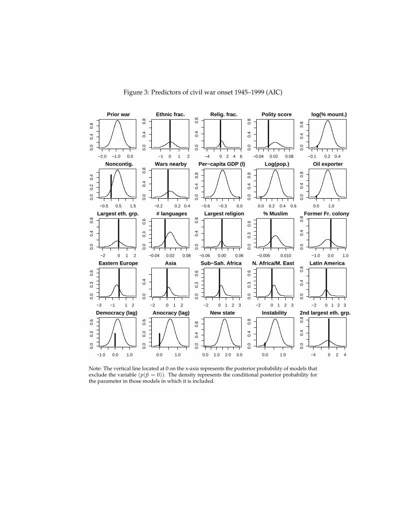
Figure 3: Predictors of civil war onset 1945–1999 (AIC)
−2.0 −1.0 0.0
0.0
0.4
0.8
Prior war
−1 0 1 2
0.0
0.4
0.8
Ethnic frac.
−4 0 2 4 6
0.0
0.4
0.8
Relig. frac.
−0.04 0.02 0.08
0.0
0.4
0.8
Polity score
−0.1 0.2 0.4
0.0
0.4
0.8
log(% mount.)
−0.5 0.5 1.5
0.0
0.2
0.4
Noncontig.
−0.2 0.2 0.4
0.0
0.4
0.8
Wars nearby
−0.6 −0.3 0.0
0.0
0.4
0.8
Per−capita GDP (l)
0.0 0.2 0.4 0.6
0.0
0.4
0.8
Log(pop.)
0.0 1.0
0.0
0.4
0.8
Oil exporter
−2 0 1 2
0.0
0.4
0.8
Largest eth. grp.
−0.04 0.02 0.08
0.0
0.3
0.6
# languages
−0.06 0.00 0.06
0.0
0.4
0.8
Largest religion
−0.005 0.010
0.0
0.3
0.6
% Muslim
−1.0 0.0 1.0
0.0
0.4
0.8
Former Fr. colony
−3 −1 1 2
0.0
0.3
0.6
Eastern Europe
−2 0 1 2
0.0
0.4
Asia
−2 0 1 2 3
0.0
0.3
0.6
Sub−Sah. Africa
−2 0 1 2 3
0.0
0.3
0.6
N. Africa/M. East
−2 0 1 2 30.
00.
40.
8
Latin America
−1.0 0.0 1.0
0.0
0.3
0.6
Democracy (lag)
0.0 1.0
0.0
0.3
0.6
Anocracy (lag)
0.0 1.0 2.0 3.0
0.0
0.4
0.8
New state
0.0 1.0
0.0
0.4
0.8
Instability
−4 0 2 4
0.0
0.4
0.8
2nd largest eth. grp.
Note: The vertical line located at 0 on the x-axis represents the posterior probability of models thatexclude the variable (p(β = 0)). The density represents the conditional posterior probability forthe parameter in those models in which it is included.
Tabl
e1:
OLS
mod
els
ofD
emoc
rati
cvo
tesh
are
inU
.S.S
enat
eca
mpa
igns
1988
–199
2A
BD
repl
icat
ion
BM
Are
anal
ysis
Red
uced
mod
elFu
llm
odel
(hyp
er-g
prio
r)M
ean
cand
.Vo
ter-
spec
ific
Mea
nca
nd.
Vote
r-sp
ecifi
cM
ean
cand
.Vo
ter-
spec
ific
Mea
nM
ean
Mea
nM
ean
Con
d.m
ean
P(β6=
0)C
ond.
mea
nP(β6=
0)(S
D)
(SD
)(S
D)
(SD
)(S
D)
(SD
)D
emoc
rati
cpr
oxim
ity
adv.
-3.1
37-2
.881
-3.0
53-2
.007
-0.2
220.
067
0.74
50.
033
(1.5
93)
(1.2
70)
(1.3
15)
(1.0
56)
(0.9
54)
(0.6
77)
Dem
ocra
tic
dire
ctio
nala
dv.
11.1
465.
729
7.95
34.
177
3.57
60.
299
2.36
30.
787
(3.3
76)
(1.6
20)
(2.8
54)
(1.3
56)
(2.0
15)
(0.8
40)
Dem
ocra
tic
incu
mbe
ncy
adv.
6.37
66.
609
1.06
01.
139
1.60
70.
194
1.29
50.
159
(1.0
92)
(1.0
54)
(1.2
01)
(1.1
89)
(1.2
42)
(1.2
37)
Dem
ocra
tic
qual
ity
adv.
5.97
25.
035
3.11
72.
378
2.96
40.
599
2.74
00.
541
(1.4
00)
(1.3
84)
(1.2
40)
(1.2
16)
(1.2
46)
(1.2
23)
Dem
ocra
tic
spen
ding
adv.
––
0.27
00.
265
0.32
381.
000.
314
1.00
(0.0
41)
(0.0
40)
(0.0
41)
(0.0
37)
Dem
ocra
tic
part
isan
adv.
––
0.05
50.
060
0.07
490.
201
0.06
610.
181
(0.0
54)
(0.0
54)
(0.0
57)
(0.0
55)
Con
stan
t54
.759
52.7
8653
.309
52.0
2851
.381
1.00
51.5
561.
00(1
.325
)(0
.892
)(1
.155
)(0
.758
)(1
.032
)(0
.764
)N
9595
9494
9494
Tabl
e2:
OLS
mod
els
ofin
cum
bent
vote
shar
esin
U.S
.Hou
seel
ecti
ons
1956
–199
6C
WB
Cre
plic
atio
nU
ncon
diti
onal
mod
els
Con
diti
onal
mod
els
All
mod
els
Coe
ffici
ent
Con
d.m
ean
P(β6=
0)C
ond.
mea
nP(β6=
0)C
ond.
mea
nP(β6=
0)(R
obus
tSE)
(SD
)(S
D)
(SD
)R
oll-
call
ideo
logi
cale
xtre
mit
y(A
DA
)-0
.070
-0.0
615
0.00
00-0
.055
00.
0000
-0.0
550
0.00
00(0
.005
)(0
.004
6)(0
.004
8)(0
.004
8)R
oll-
call
ideo
logi
cale
xtre
mit
y(D
W-N
OM
)–
-0.2
278
1.00
00-0
.224
71.
0000
-0.2
247
1.00
00(0
.015
8)(0
.015
7)(0
.015
7)Pr
esid
enti
alvo
te0.
454
0.39
961.
0000
-0.0
508
1.00
00-0
.050
81.
0000
(0.0
11)
(0.0
115)
(0.0
548)
(0.0
548)
Pres
iden
tial
vote×
extr
emit
y(A
DA
)–
–0.
1804
0.00
000.
1804
0.00
00(0
.035
4)(0
.035
4)Pr
esid
enti
alvo
te×
extr
emit
y(D
W-N
OM
)–
–0.
8952
1.00
000.
8952
1.00
00(0
.106
5)(0
.106
5)C
halle
nger
qual
ity
-0.0
53-0
.049
51.
0000
-0.0
492
1.00
00-0
.049
21.
0000
(0.0
02)
(0.0
023)
(0.0
023)
(0.0
023)
Fres
hman
-0.0
20-0
.020
31.
0000
-0.0
198
1.00
00-0
.019
81.
0000
(0.0
03)
(0.0
028)
(0.0
027)
(0.0
027)
Five
orm
ore
term
s–
-0.0
041
0.57
23-0
.003
30.
3622
-0.0
033
0.36
22(0
.002
1)(0
.002
0)(0
.002
0)In
part
y-0
.040
-0.0
594
1.00
00-0
.059
31.
0000
-0.0
593
1.00
00(0
.011
)(0
.013
1)(0
.013
1)(0
.013
1)∆
pers
onal
inco
me
0.04
20.
0426
1.00
000.
0426
1.00
000.
0426
1.00
00(c
oded
byin
part
y)(0
.003
)(0
.003
5)(0
.003
5)(0
.003
5)Pr
esid
enti
alpo
pula
rity
-0.0
44-0
.021
50.
5687
-0.0
218
0.53
97-0
.021
80.
5397
(cod
edby
inpa
rty)
(0.0
10)
(0.0
107)
(0.0
107)
(0.0
107)
Mid
term
loss
-0.0
15-0
.019
21.
0000
-0.0
196
1.00
00-0
.019
61.
0000
(cod
edby
inpa
rty)
(0.0
03)
(0.0
027)
(0.0
027)
(0.0
027)
Year
ssi
nce
1956
–0.
0025
1.00
000.
0022
1.00
000.
0022
1.00
00(0
.000
8)(0
.000
8)(0
.000
8)Ye
ars
sinc
e19
562
0.00
0028
1.00
000.
0000
471.
0000
0.00
0047
1.00
00(0
.000
049)
(0.0
0004
5)(0
.000
045)
Year
ssi
nce
1956
3–
-0.0
0000
20.
9377
-0.0
0000
20.
9737
-0.0
0000
20.
9737
(0.0
0000
1)(0
.000
001)
(0.0
0000
1)Pr
op.A
fric
anA
mer
ican
–0.
1320
1.00
000.
1054
1.00
000.
1054
1.00
00(c
oded
bypa
rty)
(0.0
077)
(0.0
083)
(0.0
083)
Prop
.vet
eran
s–
0.00
481.
0000
0.00
491.
0000
0.00
491.
0000
(cod
edby
part
y)(0
.000
6)(0
.000
6)(0
.000
6)Pr
op.f
orei
gnbo
rn–
0.19
351.
0000
0.19
151.
0000
0.19
151.
0000
(cod
edby
part
y)(0
.017
0)(0
.016
8)(0
.016
8)Pr
op.e
mpl
oyed
inm
anuf
actu
ring
-0.1
889
1.00
00-0
.174
91.
0000
-0.1
749
1.00
00(c
oded
bypa
rty)
(0.0
214)
(0.0
213)
(0.0
213)
Prop
.rur
al–
0.01
510.
3187
0.01
540.
2821
0.01
540.
2821
(cod
edby
part
y)(0
.011
5)(0
.011
4)(0
.011
4)%
unio
nw
orke
rsin
stat
e–
0.04
871.
0000
0.04
761.
0000
0.04
761.
0000
(cod
edby
part
y)(0
.008
6)(0
.008
5)(0
.008
5)C
onst
ant
0.73
90.
7675
1.00
000.
7651
1.00
000.
7651
1.00
00(0
.007
)(0
.010
2)(0
.010
1)(0
.010
1)N
6521
6521
6521
6521
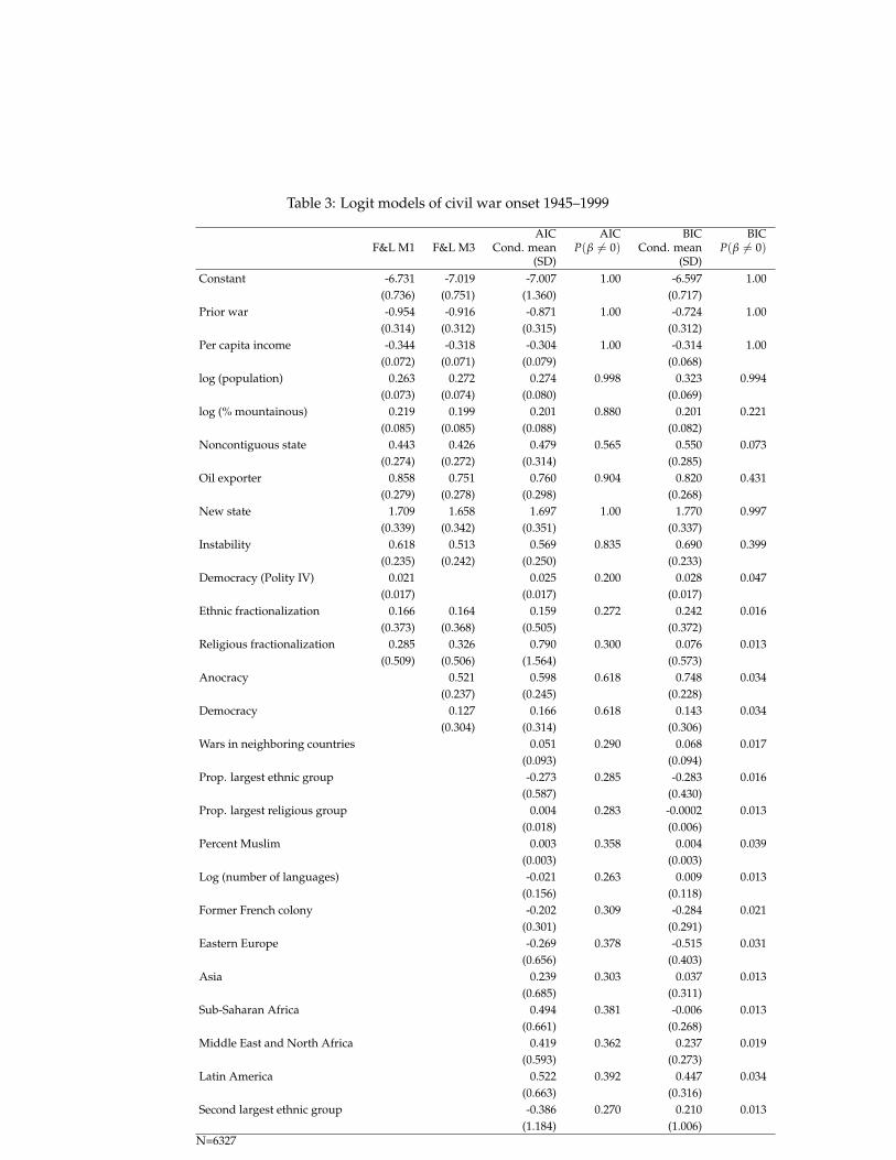
Table 3: Logit models of civil war onset 1945–1999
AIC AIC BIC BICF&L M1 F&L M3 Cond. mean P(β 6= 0) Cond. mean P(β 6= 0)
(SD) (SD)Constant -6.731 -7.019 -7.007 1.00 -6.597 1.00
(0.736) (0.751) (1.360) (0.717)Prior war -0.954 -0.916 -0.871 1.00 -0.724 1.00
(0.314) (0.312) (0.315) (0.312)Per capita income -0.344 -0.318 -0.304 1.00 -0.314 1.00
(0.072) (0.071) (0.079) (0.068)log (population) 0.263 0.272 0.274 0.998 0.323 0.994
(0.073) (0.074) (0.080) (0.069)log (% mountainous) 0.219 0.199 0.201 0.880 0.201 0.221
(0.085) (0.085) (0.088) (0.082)Noncontiguous state 0.443 0.426 0.479 0.565 0.550 0.073
(0.274) (0.272) (0.314) (0.285)Oil exporter 0.858 0.751 0.760 0.904 0.820 0.431
(0.279) (0.278) (0.298) (0.268)New state 1.709 1.658 1.697 1.00 1.770 0.997
(0.339) (0.342) (0.351) (0.337)Instability 0.618 0.513 0.569 0.835 0.690 0.399
(0.235) (0.242) (0.250) (0.233)Democracy (Polity IV) 0.021 0.025 0.200 0.028 0.047
(0.017) (0.017) (0.017)Ethnic fractionalization 0.166 0.164 0.159 0.272 0.242 0.016
(0.373) (0.368) (0.505) (0.372)Religious fractionalization 0.285 0.326 0.790 0.300 0.076 0.013
(0.509) (0.506) (1.564) (0.573)Anocracy 0.521 0.598 0.618 0.748 0.034
(0.237) (0.245) (0.228)Democracy 0.127 0.166 0.618 0.143 0.034
(0.304) (0.314) (0.306)Wars in neighboring countries 0.051 0.290 0.068 0.017
(0.093) (0.094)Prop. largest ethnic group -0.273 0.285 -0.283 0.016
(0.587) (0.430)Prop. largest religious group 0.004 0.283 -0.0002 0.013
(0.018) (0.006)Percent Muslim 0.003 0.358 0.004 0.039
(0.003) (0.003)Log (number of languages) -0.021 0.263 0.009 0.013
(0.156) (0.118)Former French colony -0.202 0.309 -0.284 0.021
(0.301) (0.291)Eastern Europe -0.269 0.378 -0.515 0.031
(0.656) (0.403)Asia 0.239 0.303 0.037 0.013
(0.685) (0.311)Sub-Saharan Africa 0.494 0.381 -0.006 0.013
(0.661) (0.268)Middle East and North Africa 0.419 0.362 0.237 0.019
(0.593) (0.273)Latin America 0.522 0.392 0.447 0.034
(0.663) (0.316)Second largest ethnic group -0.386 0.270 0.210 0.013
(1.184) (1.006)N=6327