ON INTELLIGENT DISTRICT HEATING

ON

INT

EL

LIG

EN

T D

IST

RIC

T H

EA

TIN

G

Christian Johansson

Christian Johansson

Blekinge Institute of Technology

Doctoral Dissertation Series No. 2014:07

Department of Computer Science and Engineering 2014:07

ISSN: 1653-2090

ISBN: 978-91-7295-280-5

ABSTRACTIntelligent district heating is the combination of traditional district heating engineering and mo-dern information and communication technology. A district heating system is a highly complex environment consisting of a large number of distributed entities, and this complexity and geo-graphically dispersed layout suggest that they are suitable for distributed optimization and mana-gement. However, this would in practice imply a transition from the classical production-centric perspective normally found within district heating management to a more consumer-centric per-spective.

This thesis describes a multiagent-based system which combines production, consumption and distribution aspects into a single coherent opera-tional management framework. The flexibility and robustness of the solution in industrial settings is thoroughly examined and its performance is shown to lead to significant operational, financial and environmental benefits compared to current management schemes.

2014:07

On Intelligent District Heating

Christian Johansson

Blekinge Institute of Technology Doctoral Dissertation SeriesNo 2014:07

On Intelligent District Heating

Christian Johansson

Doctoral Dissertation inComputer Science

Department of Computer Science and Engineering Blekinge Institute of Technology

SWEDEN

Psychosocial, Socio-Demographic and Health Determinants in Information Communication

Technology Use of Older-Adult

Jessica Berner

Doctoral Dissertation in Applied Health Technology

Blekinge Institute of Technology doctoral dissertation seriesNo 2014:03

Blekinge Institute of Technology

SWEDEN

Department of Health

2014 Christian Johansson Department of Computer Science and Engineering Publisher: Blekinge Institute of TechnologySE-371 79 Karlskrona, SwedenPrinted by Lenanders Grafiska, Kalmar, 2014ISBN: 978-91-7295-280-5 ISSN 1653-2090urn:nbn:se:bth-00587

”I’ve come up with a set of rules that describe our reactions to tech-nologies:

1. Anything that is in the world when you are born is normal andordinary and is just a natural part of the way the world works.

2. Anything that’s invented between when youre fifteen and thirty-five is new and exciting and revolutionary and you can probably get acareer in it.

3. Anything invented after you’re thirty-five is against the naturalorder of things.”

– Douglas Adams (1952-2001)

Abstract

Intelligent district heating is the combination of traditional district heating engineering

and modern information and communication technology. A district heating system is

a highly complex environment consisting of a large number of distributed entities, and

this complexity and geographically dispersed layout suggest that they are suitable for

distributed optimization and management. However, this would in practice imply a

transition from the classical production-centric perspective normally found within dis-

trict heating management to a more consumer-centric perspective. This thesis describes

a multiagent-based system which combines production, consumption and distribution

aspects into a single coherent operational management framework. The flexibility and

robustness of the solution in industrial settings is thoroughly examined and its perfor-

mance is shown to lead to significant operational, financial and environmental benefits

compared to current management schemes.

i

Acknowledgments

This thesis is dedicated to my friend and colleague Dr Fredrik Wernstedt. With-out him none of this would have been possible. He is dearly missed.

I would like to convey my deepest gratitude and respect to Professor PaulDavidsson who not only served as my supervisor but also encouraged and chal-lenged me throughout the years leading up to this thesis.

Furthermore, I would like to thank everyone at Noda Intelligent Systemsfor their support over the years. I would especially like to acknowledge MikaelGanehag Brorsson and Markus Bergkvist for going (and keeping on going) thatextra mile.

I would especially like to thank Katya for putting up with me during thewriting of this thesis. Thank you for being part of my life.

To my family and friends for providing me with encouragement and motiva-tion.

The research leading up to this thesis was financially supported by BlekingeInstitute of Technology, the Swedish District Heating Association and the Euro-pean Spallation Source.

Karlshamn, April 2014Christian Johansson

iii

Preface

In 2001 the ABSINTHE (Agent-Based Monitoring and Control of District Heat-ing Systems) project was started by Professor Paul Davidsson and Dr FredrikWernstedt at Blekinge Institute of Technology, although their initial research con-cerning distributed control in district heating systems started already in 1999.The ABSINTHE research project was jointly funded by Blekinge Institute ofTechnology, Vinnova and Cetetherm AB, and dealt with the fundamental prin-ciples of applying multi-agent based solutions to the problem of operational re-source management within district heating systems. The project resulted in thedoctoral dissertation ”Multi-Agent Systems for Distributed Control of DistrictHeating Systems” by Fredrik Wernstedt in 2005.

The work described in this doctoral thesis can be seen as a continuation ofthe work previously achieved during the ABSINTHE project, although with ahigher focus on actual real-time implementations of the studied solutions. Dur-ing the work for this thesis it has become apparent that real world domain ofdistrict heating systems and energy systems in general is much more complexthan assumed in the early stages of the ABSINTHE project. This thesis is astep towards describing how to handle that complexity while implementing op-erational demand side management for real life applications.

This thesis comprises twelve papers that are listed below and will be referencedin the following text by their associated Roman numeral. The author of this thesishas been the main contributor to papers I, IV, V, VI, VII, VIII, IX, X, XI andXII and contributing author for papers II and III. The author has contributed toall papers in relation to conducting experiments, analysing data and writing thepaper. All of the papers, except XI and XII, have previously been accepted forpublication. Paper XI and XII is under review. All papers have been reformattedin order to conform to the thesis template.

I. Johansson, C. & Wernstedt, F. (2005). Dynamic Simulation of DistrictHeating Systems. The 3rd European Simulation and Modelling Confer-ence, Oporto, Portugal.

v

II. Wernstedt, F., Davidsson, P. & Johansson, C. (2007). Demand Side Man-agement in District Heating Systems. The 6th International Conferenceon Autonomous Agents and Multiagent Systems, Honolulu, Hawaii.

III. Wernstedt, F. & Johansson, C. (2008). Intelligent distributed load con-trol. The 11th International Symposium on District Heating and Cooling,Reykjavik, Iceland.

IV. Johansson, C., Wernstedt, F. & Davidsson, P. (2010). A Case Study onAvailability of Sensor Data in Agent Cooperation. Computer Science andInformation Systems, vol 7, no 3.

V. Johansson, C., Wernstedt, F. & Davidsson, P. (2010). Deployment ofAgent Based Load Control in District Heating Systems. The 1st Inter-national Workshop on Agent Technologies for Energy Systems, Toronto,Canada.

VI. Johansson, C. & Wernstedt, F. (2010). Heat Load Reductions and theireffect on Energy Consumption. The 12th International Symposium onDistrict Heating and Cooling, Tallinn, Estonia.

VII. Johansson, C., Wernstedt, F. & Davidsson, P. (2012). Combined Heatand Power Generation using Smart Heat Grid. The 4th InternationalConference on Applied Energy, Suzhou, China.

VIII. Johansson, C., Wernstedt, F. & Davidsson, P. (2012). Smart Heat Gridon an Intraday Power Market. The 3rd International Workshop on AgentTechnologies for Energy Systems, Valencia, Spain.

IX. Johansson, C. & Wernstedt, F. (2012). N-dimensional Fault Detectionand Operational Analysis with Performance Metrics. The 13th Interna-tional Symposium on District Heating and Cooling, Copenhagen, Den-mark.

X. Johansson, C., Wernstedt, F. & Davidsson, P. (2012). Distributed Ther-mal Storage Using Multiagent Systems. The 1st International Conferenceon Agreement Technologies, Dubrovnik, Croatia.

XI. Johansson, C. & Davidsson, P. (2014). A Smart Heat Grid Frameworkusing Intelligent Software Agents. in review

XII. Johansson, C. & Davidsson, P. (2014). A dynamic simulation of theproduction, distribution and consumption of district heating systems: Averification study of Dhemos unpublished report

In addition to the papers included in the actual thesis, the following papers arealso related to the thesis. These papers are the results of various research projectsfinanced by the Swedish District Heating Association and they are published astechnical reports in Swedish.

XIII. Wernstedt, F., Johansson, C. & Wollerstrand, J. (2008). Sankta re-turtemperaturer genom laststyrning. Report 2008:2, Svensk Fjarrvarme.(”Lowered return temperatures through load control”, in Swedish)

XIV. Wernstedt, F. & Johansson, C. (2009). Demonstrationsprojekt inom last-och effektstyrning. Report 2009:26, Svensk Fjarrvarme. (”Demonstrationproject in heat-load control”, in Swedish)

XV. Johansson, C. & Wernstedt, F. (2010). Forstudie infor dynamisk fjarrvarmes-imulator. Report 2010:1, Svensk Fjarrvarme. (”Pre-study of dynamicdistrict heating simulator”, in Swedish)

XVI. Johansson, C. & Wernstedt, F. (2012). Dynamisk Fjarrvarmesimulator ipraktiken. Report 2012:1, Svensk Fjarrvarme. (”Dynamic district heat-ing simulator in practice”, in Swedish)

Contents

Abstract i

Acknowledgments iii

Preface v

1 Introduction 1

1.1 Background . . . . . . . . . . . . . . . . . . . . . . . . . . . . . . . . . . 3

1.1.1 Multi-Agent Systems . . . . . . . . . . . . . . . . . . . . . . . . . 3

1.1.2 District Heating . . . . . . . . . . . . . . . . . . . . . . . . . . . 5

1.1.3 Smart Grid Technology . . . . . . . . . . . . . . . . . . . . . . . 7

1.1.4 Simulation . . . . . . . . . . . . . . . . . . . . . . . . . . . . . . 8

1.1.5 Heat Load Prediction . . . . . . . . . . . . . . . . . . . . . . . . 8

1.2 Research Approach . . . . . . . . . . . . . . . . . . . . . . . . . . . . . . 9

1.2.1 Research Questions . . . . . . . . . . . . . . . . . . . . . . . . . . 9

1.2.2 Research Method . . . . . . . . . . . . . . . . . . . . . . . . . . . 10

1.2.3 Thesis contribution . . . . . . . . . . . . . . . . . . . . . . . . . . 11

1.2.4 Related reports . . . . . . . . . . . . . . . . . . . . . . . . . . . . 15

1.3 Conclusions . . . . . . . . . . . . . . . . . . . . . . . . . . . . . . . . . . 16

1.4 Future Work . . . . . . . . . . . . . . . . . . . . . . . . . . . . . . . . . 17

2 Paper I - Dynamic simulation of district heating systems 19

2.1 Keywords . . . . . . . . . . . . . . . . . . . . . . . . . . . . . . . . . . . 19

2.2 Introduction . . . . . . . . . . . . . . . . . . . . . . . . . . . . . . . . . . 19

2.3 District heating systems . . . . . . . . . . . . . . . . . . . . . . . . . . . 20

2.4 Dhemos . . . . . . . . . . . . . . . . . . . . . . . . . . . . . . . . . . . . 21

2.4.1 Consumption . . . . . . . . . . . . . . . . . . . . . . . . . . . . . 21

2.5 Production . . . . . . . . . . . . . . . . . . . . . . . . . . . . . . . . . . 25

2.6 Distribution . . . . . . . . . . . . . . . . . . . . . . . . . . . . . . . . . . 26

2.7 Simulation of Gavle district heating system . . . . . . . . . . . . . . . . 28

2.8 Conclusions and future work . . . . . . . . . . . . . . . . . . . . . . . . 29

ix

3 Paper II - Demand side management in district heating systems 313.1 Keywords . . . . . . . . . . . . . . . . . . . . . . . . . . . . . . . . . . . 313.2 Introduction . . . . . . . . . . . . . . . . . . . . . . . . . . . . . . . . . . 31

3.2.1 Background . . . . . . . . . . . . . . . . . . . . . . . . . . . . . . 323.3 MAS architecture . . . . . . . . . . . . . . . . . . . . . . . . . . . . . . . 343.4 Agent behaviour . . . . . . . . . . . . . . . . . . . . . . . . . . . . . . . 37

3.4.1 Consumer agent . . . . . . . . . . . . . . . . . . . . . . . . . . . 383.4.2 Producer agent . . . . . . . . . . . . . . . . . . . . . . . . . . . . 393.4.3 Cluster agent . . . . . . . . . . . . . . . . . . . . . . . . . . . . . 40

3.5 Deployed system . . . . . . . . . . . . . . . . . . . . . . . . . . . . . . . 413.5.1 Results . . . . . . . . . . . . . . . . . . . . . . . . . . . . . . . . 423.5.2 Return of investment . . . . . . . . . . . . . . . . . . . . . . . . . 443.5.3 Discussion . . . . . . . . . . . . . . . . . . . . . . . . . . . . . . . 45

3.6 Conclusions . . . . . . . . . . . . . . . . . . . . . . . . . . . . . . . . . . 453.7 Future work . . . . . . . . . . . . . . . . . . . . . . . . . . . . . . . . . . 463.8 Acknowledgements . . . . . . . . . . . . . . . . . . . . . . . . . . . . . . 46

4 Paper III - Intelligent distributed load control 474.1 Introduction . . . . . . . . . . . . . . . . . . . . . . . . . . . . . . . . . . 47

4.1.1 Demand side management quality filter . . . . . . . . . . . . . . 494.2 Demand side management quality filter for district heating systems . . . 494.3 Field test . . . . . . . . . . . . . . . . . . . . . . . . . . . . . . . . . . . 504.4 Results . . . . . . . . . . . . . . . . . . . . . . . . . . . . . . . . . . . . . 534.5 Discussion . . . . . . . . . . . . . . . . . . . . . . . . . . . . . . . . . . . 564.6 Conclusions . . . . . . . . . . . . . . . . . . . . . . . . . . . . . . . . . . 58

5 Paper IV - A case study on availability of sensor data in agent coop-eration 595.1 Keyworks . . . . . . . . . . . . . . . . . . . . . . . . . . . . . . . . . . . 595.2 Introduction . . . . . . . . . . . . . . . . . . . . . . . . . . . . . . . . . . 60

5.2.1 Problem domain . . . . . . . . . . . . . . . . . . . . . . . . . . . 605.2.2 Problem description . . . . . . . . . . . . . . . . . . . . . . . . . 61

5.3 The agent system . . . . . . . . . . . . . . . . . . . . . . . . . . . . . . . 635.3.1 Agents . . . . . . . . . . . . . . . . . . . . . . . . . . . . . . . . . 635.3.2 Agent goal . . . . . . . . . . . . . . . . . . . . . . . . . . . . . . 655.3.3 Auction process . . . . . . . . . . . . . . . . . . . . . . . . . . . . 665.3.4 Levels of agent knowledge . . . . . . . . . . . . . . . . . . . . . . 66

5.4 The experiment . . . . . . . . . . . . . . . . . . . . . . . . . . . . . . . . 685.4.1 Reference data . . . . . . . . . . . . . . . . . . . . . . . . . . . . 685.4.2 Utility evalution . . . . . . . . . . . . . . . . . . . . . . . . . . . 685.4.3 Availability of sensor data . . . . . . . . . . . . . . . . . . . . . . 705.4.4 Simulation . . . . . . . . . . . . . . . . . . . . . . . . . . . . . . 71

5.5 Results . . . . . . . . . . . . . . . . . . . . . . . . . . . . . . . . . . . . . 715.5.1 Control strategy . . . . . . . . . . . . . . . . . . . . . . . . . . . 725.5.2 Agent buffer usage . . . . . . . . . . . . . . . . . . . . . . . . . . 73

5.6 Discussion . . . . . . . . . . . . . . . . . . . . . . . . . . . . . . . . . . . 755.7 Conclusions . . . . . . . . . . . . . . . . . . . . . . . . . . . . . . . . . . 765.8 Future work . . . . . . . . . . . . . . . . . . . . . . . . . . . . . . . . . . 775.9 Acknowledgements . . . . . . . . . . . . . . . . . . . . . . . . . . . . . . 78

6 Paper V - Deployment of agent based load control in district heatingsystems 796.1 Keywords . . . . . . . . . . . . . . . . . . . . . . . . . . . . . . . . . . . 806.2 Introduction . . . . . . . . . . . . . . . . . . . . . . . . . . . . . . . . . . 80

6.2.1 Load control . . . . . . . . . . . . . . . . . . . . . . . . . . . . . 806.3 System description . . . . . . . . . . . . . . . . . . . . . . . . . . . . . . 82

6.3.1 Multi-agent system . . . . . . . . . . . . . . . . . . . . . . . . . . 836.3.2 Additional hardware and software . . . . . . . . . . . . . . . . . 85

6.4 Deployed system . . . . . . . . . . . . . . . . . . . . . . . . . . . . . . . 866.4.1 Results . . . . . . . . . . . . . . . . . . . . . . . . . . . . . . . . 866.4.2 Indoor climate . . . . . . . . . . . . . . . . . . . . . . . . . . . . 906.4.3 Available load control ability . . . . . . . . . . . . . . . . . . . . 916.4.4 Cost-benefit analysis . . . . . . . . . . . . . . . . . . . . . . . . . 93

6.5 Discussion . . . . . . . . . . . . . . . . . . . . . . . . . . . . . . . . . . . 946.6 Conclusions . . . . . . . . . . . . . . . . . . . . . . . . . . . . . . . . . . 946.7 Future work . . . . . . . . . . . . . . . . . . . . . . . . . . . . . . . . . . 976.8 Acknowledgements . . . . . . . . . . . . . . . . . . . . . . . . . . . . . . 97

7 Paper VI - Heat load reductions and their effect on energy consump-tion 997.1 Introduction . . . . . . . . . . . . . . . . . . . . . . . . . . . . . . . . . . 99

7.1.1 Night time set-back . . . . . . . . . . . . . . . . . . . . . . . . . 1007.1.2 Demand side management and load control . . . . . . . . . . . . 1017.1.3 Previous work . . . . . . . . . . . . . . . . . . . . . . . . . . . . . 101

7.2 Experimental method . . . . . . . . . . . . . . . . . . . . . . . . . . . . 1027.3 Results . . . . . . . . . . . . . . . . . . . . . . . . . . . . . . . . . . . . . 1037.4 Discussion . . . . . . . . . . . . . . . . . . . . . . . . . . . . . . . . . . . 1107.5 Conclusions . . . . . . . . . . . . . . . . . . . . . . . . . . . . . . . . . . 1117.6 Future work . . . . . . . . . . . . . . . . . . . . . . . . . . . . . . . . . . 1127.7 Acknowledgement . . . . . . . . . . . . . . . . . . . . . . . . . . . . . . . 112

8 Paper VII - Combined heat and power generation using smart heatgrid 1138.1 Introduction . . . . . . . . . . . . . . . . . . . . . . . . . . . . . . . . . . 1148.2 Related work . . . . . . . . . . . . . . . . . . . . . . . . . . . . . . . . . 1168.3 Load control in buildings . . . . . . . . . . . . . . . . . . . . . . . . . . 1178.4 Heat load synchronization . . . . . . . . . . . . . . . . . . . . . . . . . . 1198.5 Market based heat load allocation using agent technology . . . . . . . . 1228.6 Experimental set-up . . . . . . . . . . . . . . . . . . . . . . . . . . . . . 1248.7 Results . . . . . . . . . . . . . . . . . . . . . . . . . . . . . . . . . . . . . 125

8.8 Discussion . . . . . . . . . . . . . . . . . . . . . . . . . . . . . . . . . . . 1288.9 Conclusions . . . . . . . . . . . . . . . . . . . . . . . . . . . . . . . . . . 1308.10 Future work . . . . . . . . . . . . . . . . . . . . . . . . . . . . . . . . . . 1308.11 Acknowledgement . . . . . . . . . . . . . . . . . . . . . . . . . . . . . . . 131

9 Paper VIII - Smart heat grid on an intraday power market 1339.1 Introduction . . . . . . . . . . . . . . . . . . . . . . . . . . . . . . . . . . 1349.2 Related work . . . . . . . . . . . . . . . . . . . . . . . . . . . . . . . . . 1369.3 Multi-agent system overview . . . . . . . . . . . . . . . . . . . . . . . . 137

9.3.1 Consumer agent . . . . . . . . . . . . . . . . . . . . . . . . . . . 1389.3.2 Producer agent . . . . . . . . . . . . . . . . . . . . . . . . . . . . 1429.3.3 Market agent . . . . . . . . . . . . . . . . . . . . . . . . . . . . . 144

9.4 Experimental set-up . . . . . . . . . . . . . . . . . . . . . . . . . . . . . 1459.5 Results . . . . . . . . . . . . . . . . . . . . . . . . . . . . . . . . . . . . . 1469.6 Discussion . . . . . . . . . . . . . . . . . . . . . . . . . . . . . . . . . . . 1489.7 Conclusions . . . . . . . . . . . . . . . . . . . . . . . . . . . . . . . . . . 1509.8 Future work . . . . . . . . . . . . . . . . . . . . . . . . . . . . . . . . . . 1509.9 Acknowledgement . . . . . . . . . . . . . . . . . . . . . . . . . . . . . . . 150

10 Paper IX - N-dimensional fault detection and operational analysiswith performance metrics 15110.1 Introduction . . . . . . . . . . . . . . . . . . . . . . . . . . . . . . . . . . 15210.2 Related work . . . . . . . . . . . . . . . . . . . . . . . . . . . . . . . . . 15210.3 N-dimensional analysis . . . . . . . . . . . . . . . . . . . . . . . . . . . . 15410.4 Outliers . . . . . . . . . . . . . . . . . . . . . . . . . . . . . . . . . . . . 15510.5 Parallel coordinates and scatter plot matrices . . . . . . . . . . . . . . . 15510.6 Performance metrics . . . . . . . . . . . . . . . . . . . . . . . . . . . . . 15610.7 Results . . . . . . . . . . . . . . . . . . . . . . . . . . . . . . . . . . . . . 158

10.7.1 Operational analysis . . . . . . . . . . . . . . . . . . . . . . . . . 15910.7.2 Outlier detection . . . . . . . . . . . . . . . . . . . . . . . . . . . 161

10.8 Discussion . . . . . . . . . . . . . . . . . . . . . . . . . . . . . . . . . . . 16210.9 Conclusions . . . . . . . . . . . . . . . . . . . . . . . . . . . . . . . . . . 16510.10Future work . . . . . . . . . . . . . . . . . . . . . . . . . . . . . . . . . . 16510.11Acknowledgement . . . . . . . . . . . . . . . . . . . . . . . . . . . . . . . 165

11 Paper X - Distributed thermal storage using multiagent systems 16711.1 Introduction . . . . . . . . . . . . . . . . . . . . . . . . . . . . . . . . . . 16811.2 Related work . . . . . . . . . . . . . . . . . . . . . . . . . . . . . . . . . 17011.3 Multi-agent system overview . . . . . . . . . . . . . . . . . . . . . . . . 171

11.3.1 Heat block value . . . . . . . . . . . . . . . . . . . . . . . . . . . 17311.3.2 Consumer agent asset . . . . . . . . . . . . . . . . . . . . . . . . 17411.3.3 Auction process . . . . . . . . . . . . . . . . . . . . . . . . . . . . 175

11.4 Experimental set-up . . . . . . . . . . . . . . . . . . . . . . . . . . . . . 17711.5 Results . . . . . . . . . . . . . . . . . . . . . . . . . . . . . . . . . . . . . 17811.6 Discussion . . . . . . . . . . . . . . . . . . . . . . . . . . . . . . . . . . . 180

11.7 Conclusions . . . . . . . . . . . . . . . . . . . . . . . . . . . . . . . . . . 18111.8 Future work . . . . . . . . . . . . . . . . . . . . . . . . . . . . . . . . . . 18111.9 Acknowledgements . . . . . . . . . . . . . . . . . . . . . . . . . . . . . . 181

12 Paper XI - A smart heat grid framework using intelligent softwareagents 18312.1 Introduction . . . . . . . . . . . . . . . . . . . . . . . . . . . . . . . . . . 18312.2 System overview . . . . . . . . . . . . . . . . . . . . . . . . . . . . . . . 18512.3 Implementation . . . . . . . . . . . . . . . . . . . . . . . . . . . . . . . . 19112.4 Results and discussion . . . . . . . . . . . . . . . . . . . . . . . . . . . . 19212.5 Conclusions . . . . . . . . . . . . . . . . . . . . . . . . . . . . . . . . . . 19612.6 Acknowledgments . . . . . . . . . . . . . . . . . . . . . . . . . . . . . . . 197

13 Paper XII - A dynamic simulation of the production, distributionand consumption of district heating systems: A verification study ofDhemos 19913.1 Simulation system overview . . . . . . . . . . . . . . . . . . . . . . . . . 200

13.1.1 The Dhemos simulation framework . . . . . . . . . . . . . . . . . 20013.1.2 Implementation of the Dhemos software package . . . . . . . . . 20413.1.3 Related simulation studies . . . . . . . . . . . . . . . . . . . . . . 205

13.2 Experimental set-up . . . . . . . . . . . . . . . . . . . . . . . . . . . . . 20713.3 Results . . . . . . . . . . . . . . . . . . . . . . . . . . . . . . . . . . . . . 20713.4 Discussion . . . . . . . . . . . . . . . . . . . . . . . . . . . . . . . . . . . 20913.5 Conclusions . . . . . . . . . . . . . . . . . . . . . . . . . . . . . . . . . . 21013.6 Acknowledgements . . . . . . . . . . . . . . . . . . . . . . . . . . . . . . 210

Bibliography 211

xiii

xiv

Chapter 1

Introduction

The district heating industry has a long tradition and now-a-days plays a majorrole in heat distribution in many countries in Northern and Eastern Europe withexpanding markets in Asia and North America (Constinescu, 2007). In an agewere all energy systems within our society are scrutinized, the district heatingconcept continues to thrive and expand based on the knowledge that it is finan-cially advantageous and environmentally sound. By Intelligent District Heatingwe refer to the merging of modern information and communication technologywith traditional district heating systems, in order to improve the operationalfunctionality of the system. Throughout this thesis the assumption that sucha merger is technically, financially and environmentally beneficial has been ex-plored.

A district heating system is at the basic level a collection of interacting or sep-arate control loop feedback systems. In order to make such a system ”intelligent”one needs to take into account all parts of this loop. In the context of this thesis,three major parts of this loop can be identified: (i) measure, (ii) analyse and(iii) act. These parts exist on the local consumer level as well as on system wideproduction and distribution levels, and they are continuously reiterated withinthe process. Each of these parts can be also mapped to three basic notions ofwhat entitles an intelligent system (Wechsler, 1944).

� The ability to perceive ones environment (measure)

� The ability to reach informed conclusions based on the perceived input(analyse)

� The ability to act based on those conclusions (act)

It is the conclusion of this thesis that all these three aspects of the system hasto be present in order to achieve a level of automation approaching something

1

that can be characterised as intelligent. However, it is common to see energysystems being labelled as smart or intelligent based solely on the mere existenceof remotely accessible metering equipment even though such a system barely evenincorporates the first of the three parts of the loop.

In order to implement a system capable of handling all three parts of the intel-ligence loop described above a distributed multiagent-based framework has beendeveloped. The idea that a multiagent approach is appropriate for district heat-ing systems stems from the fact that most such systems consist of geographicallydistributed autonomous entities that interact in complex ways. The distributionmedium in itself also applies certain time dependant constraints on the system,i.e. as opposed to electricity, water does not move at the speed of light. This leadsto a situation where the distribution of the heat can take several hours depend-ing on the geographical location of the consumers in relation to the productionplants. This combination of physically dispersed hardware nodes and inherenttime-dependency makes for a complex situation which further strengthens the no-tion that a distributed perspective is suitable in which the calculations involvedcan be divided among several computational nodes (Parunak, 1998). Further-more, district heating systems consists of a multitude of consumers and producerswho might not want to share all their operational and financial information on aglobal system wide scale just in order to achieve some optimal operational status.Together these observations lead to the hypothesis that distributed systems ingeneral and a multiagent-based solution in particular is suitable for this specificproblem domain.

The general architecture is based on two types of agents which are mod-elled based on the characteristics of a consumer substation and a productionplant. Normally a consumer wants to use as little energy as possible while stillmaintaining an acceptable indoor temperature in the buildings connected to thesubstation, while a utility or energy company usually wants to optimize the pro-duction in relation to financial and operational aspects. By modelling the agentsthis way it is possible to assign these sometimes conflicting system goals to twodifferent agent types which in the context of a multiagent system will act in orderto achieve and maintain a balance between these goals. Thus, each physical sub-station in the district heating system is assigned a consumer agent with the maingoal of maintaining an acceptable quality of service. Similarly, each productionplant is assigned a producer agent which will act in order to optimize the energyusage from financial, technical and/or environmental aspects. In addition to thisthe system also includes a market agent which acts as a mediator between theproducer and consumer agents.

Throughout this thesis variations of this basic multiagent architecture havebeen implemented and evaluated in order to find suitable techniques for dis-tributed control of district heating systems. Even during the early days of the

2

ABSINTHE project, it became apparent that there was a need for simulationand modelling tools. Using such tools was the only way to test and evaluatethe multiagent system before any appropriate hardware platform could be devel-oped. Unfortunately, there were no available simulation tools capable of handlingthe complexity of dynamic simulations in a system which combined production,distribution and consumption behavioural models. As a consequence, this thesisalso covers the development of simulation and modelling tools in order to supportthe primary work on the multiagent system.

The thesis consists of two major parts; the introductory section and a numberof publications. In the introductory section the research area is introduced andpresented together with a walk-through of the content and contribution of thedifferent papers in relation to the research questions. The chapters followingthe introduction consist of journal articles and conference papers that have beenpublished or currently are under review.

1.1 Background

The primary area of research for this thesis is Computer Science in general andagent technology and artificial intelligence applications in particular. However,the application area is district heating systems and and in order to cover theproblem domain at hand several research areas have been interwoven into aninterdisciplinary whole. By combining Computer Science with aspects of Opera-tions Research, Economics, Energy Systems, Automation and Physics the thesisdevelops the framework for intelligent district heating. The resulting work al-ternates between being published through venues related to agent systems orsimulation techniques to district heating conferences. Since the papers are pub-lished in fora aimed at different audiences, the presentational style can differslightly from paper to paper. All these areas are, however, related in the factthat they form conjoined, albeit diverse, tools used in the evolution of intelligentdistrict heating systems.

1.1.1 Multi-Agent Systems

The software agent paradigm is an underlying theme throughout this thesis as itis used to design the framework on which the whole intelligent district heatingsystem is based. A software agent can be seen as a computer program that iscapable of autonomous and independent action based on the agents internal andexternal perceptions. As such they present a flexible way of structuring applica-tions around autonomous and communicative components in open and dynamicenvironments. Agents are often used in systems handling distributed data and

3

communication, especially when there are constraints regarding integrity and pri-vacy (Parunak, 1998). An agent can also interact with other agents in so calledmultiagent systems. This interaction can be either competitive or collaborativein nature, or a combination of the two. In many ways agents can be seen as analo-gies to physical entities and the agent paradigm tries to capture human notionssuch as trust, dependence, norms, reputation and other social concepts in or-der to take into account and model the structures forming relationships betweenindividuals and organizations. The agent framework provides a basis for imple-menting interaction between computers, machines and human operators (Weiss,2000a).

A common way to implement multi-agent systems is to use market processanalogies based on traditional supply and demand mechanisms (Braeutigam,2010). In such a situation the agents are bound by a protocol through whichto interact but they are free to choose their own strategies in order to succeedon the market. As in economic theory the ’ supply and demand mechanism inmulti-agent systems provide a way to find self-balancing system behaviour. Thetheory of supply and demand is readily adaptable to the district heating domainas the consumer and production entities form obvious analogies providing supplyand demand in the network. Economic theory provides a solid framework forintroducing efficient methods for allocation and distribution of resources amonga group of agents (Ygge & Akkermans, 1996).

Agent-based software technologies form a powerful template for implementingintelligent behaviour in a variety of situations, not least in distributed environ-ments such as Internet-based software, robotics or industrial systems (Russel &Norvig, 1995). Industrial applications are in many ways the direct opposite oftext book examples as the real world is highly unpredictable and complex. Thisis also true in district heating systems which also adds another level of complex-ity in the form of a high dependence on the physical infrastructure for sensoryequipment and communication. In a district heating system the agents must becapable of functioning in a real-time environment even considering faulty or in-complete data. This is true for most type of large scale energy systems such aselectrical power grids where agent-like mechanisms can be used to identify mal-functioning in switches and relays, handle alarm messages and implement peakload management (Jennings et al., 1996).

Since we approach district heating systems from a distributed viewpoint it isconvenient to use multi-agent systems as a template for implementing intelligentbehaviour in the system. In our implementation we equip each consumer nodewith an separate agent, as well as incorporating producer agents in the system.All these agents interact in a multi-agent system in order to achieve the goals setforth by the distributed control policies.

4

1.1.2 District Heating

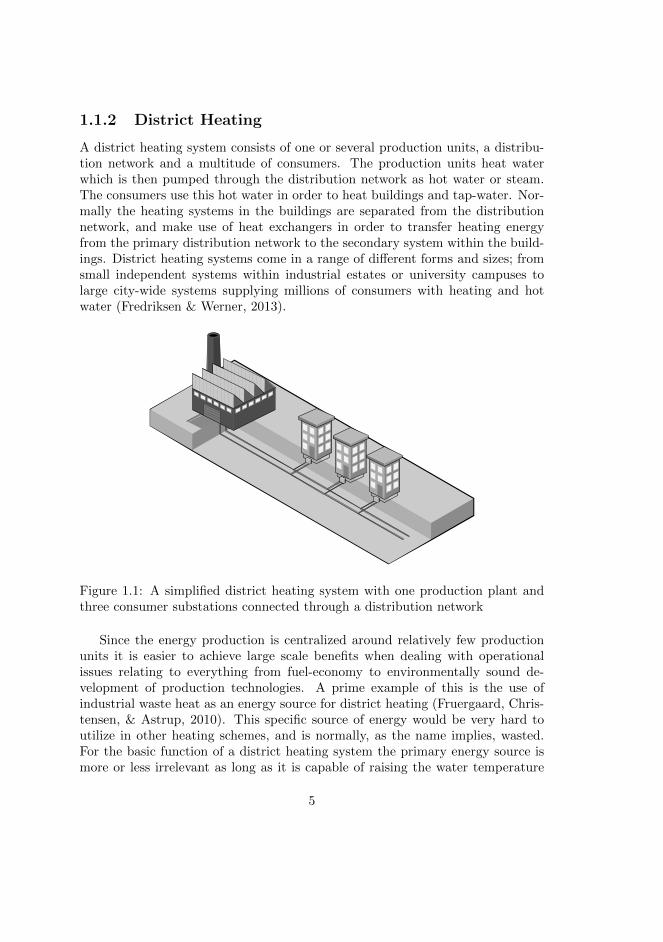
A district heating system consists of one or several production units, a distribu-tion network and a multitude of consumers. The production units heat waterwhich is then pumped through the distribution network as hot water or steam.The consumers use this hot water in order to heat buildings and tap-water. Nor-mally the heating systems in the buildings are separated from the distributionnetwork, and make use of heat exchangers in order to transfer heating energyfrom the primary distribution network to the secondary system within the build-ings. District heating systems come in a range of different forms and sizes; fromsmall independent systems within industrial estates or university campuses tolarge city-wide systems supplying millions of consumers with heating and hotwater (Fredriksen & Werner, 2013).

Figure 1.1: A simplified district heating system with one production plant andthree consumer substations connected through a distribution network

Since the energy production is centralized around relatively few productionunits it is easier to achieve large scale benefits when dealing with operationalissues relating to everything from fuel-economy to environmentally sound de-velopment of production technologies. A prime example of this is the use ofindustrial waste heat as an energy source for district heating (Fruergaard, Chris-tensen, & Astrup, 2010). This specific source of energy would be very hard toutilize in other heating schemes, and is normally, as the name implies, wasted.For the basic function of a district heating system the primary energy source ismore or less irrelevant as long as it is capable of raising the water temperature

5

to the needed level. One of the main advantages with district heating is indeedthis ability use different types of primary energy sources such as biomass, fossilfuel, geothermal heat, natural gas or nuclear powered heating.

When building new production units in district heating systems it is manytimes advantageous to invest in so called combined heat and power generation.Such a production unit generates electrical power while simultaneously generatingheat. The electrical power can be sold on the power grid while the heat is usedfor the connected district heating system. In such a system water is turned intosteam which is used in a turbine connected to a generator in order to generateelectricity. The steam is then cooled by transferring its heat to the water in thedistrict heating system. By combining these two processes it is possible to achievea very high level of energy efficiency which is why such production solutions arebecoming increasingly popular (Horlock, 2008).

One challenge in district heating systems is that the heat demand is not al-ways correlated with an optimal production scheme. Many of the primary energysources used in district heating benefit from an even and predictable heat load.However, the heat demand is in practice influenced by both outdoor tempera-ture dependant behaviour and social behaviour which in combination can causeuneven as well as unpredictable heat demand. Due to this most district heatingsystems include one or several peak load boilers used primarily to bridge devia-tions between heat demand and heat generation. Normally peak load boilers arefuelled by fossil fuel such as oil and natural gas, which are easy and efficient to usealthough they are more expensive than most base load fuels. Another commonsolution for this problem is to use large storage tanks where hot water can bestored temporarily in order to buffer energy for peak loads a few hours ahead.However such storage tanks are somewhat inflexible in operation and they are ex-pensive to build. Intelligent district heating in the context presented in this thesiscan in many instances be a financially and technically sound complement, or evenin some cases replacement, for such traditional solutions (Olsson Ingvarsson &Werner, 2008).

District heating as a technology has been around for a long time, and there hasbeen numerous developments made in order to increase the operational efficiencyfrom financial and environmental perspectives. However, the primary focus hasusually always been on the production side of the system, while the distributionand consumption part of the system has normally been treated more or less as ablack-box in regards to operational management. In the future an increased focuson system-wide coordination and optimization will most likely evolve, where allaspects of the entire system will need to be incorporated as dynamic and timedependant parts of the overall control scheme. As consumers grow evermoreaware of energy costs, energy producers will have to develop new business modelsin order to meet the changing demands of the market.

6

1.1.3 Smart Grid Technology

The smart grid concept is usually used in relation to electrical power grids, andis defined as a grid that uses modern information and communication equipmentin order to gather and act on data related to the operation of the grid. Thebasic idea is that by using such technology it will be possible to manage thegrid in a more efficient manner and by doing so save energy and create condi-tions for more sustainable energy systems (Braun, 2003). Smart grid technologyis usually seen as an important part of a sustainable future since many of theincreasingly popular environmentally friendly energy sources are harder to man-age than traditional fuels such as fossil fuel or nuclear power. Wind, solar andwave power are examples of such intermittent energy sources causing operationalchallenges when implemented on a large scale due to their unpredictability andother shortcomings from an energy carrier perspective. The situation is similarwithin district heating technology considering for example the extensive use ofbiomass and industrial waste heat. The simple fact is that such energy sourcesare not as manageable as fossil fuel, irrespective of their financial or environ-mental benefits. In the context of this thesis a smart grid uses information andcommunication technology in order to coordinate the demands and requirementsof all participating actors from technical, financial and environmental aspects.When implemented in a district heating system this is called a smart heat grid.In some literature such systems are called smart thermal grids in order to includecooling as well as heating technologies. A smart heat grid adds another degreeof control to the traditional demand-driven management in a district heatingsystem. Instead of simple being able to react on the heat demand, the energycompany can manage and control the heat demand.

One of the primary objectives of a smart heat grid is to implement a frameworkfor demand side management and operational load control, just like in a generalsmart grid (Torriti, 2012). Demand side management and load control lie at thecore of the consumption oriented approach to operational management withindistrict heating systems. The basic idea is to be able to control the heat loaddemand at the consumer level and thus introduce another dimension of controlfor the energy producer. These techniques can be implemented directly as wellas indirectly. An indirect approach might, for example, involve using a certainpricing scheme with differentiable energy cost in relation to the current heat loadusage. Such pricing might be used in order to mitigate peak load problems withindistrict heating systems (Newsham & Bowker, 2010). The fundamental problemwith such indirect approaches is that even though the consumer might be ableto observe what is going on, they usually have no means to do anything aboutit until it is to late. Operational load control or demand side management iswhen the energy producer is able, within certain limits, to directly control theheat load usage by remote means. Direct approaches might be more appropriate

7

for operational management, but are, on the other hand, much more difficult toimplement since they tend to require considerable investments in hardware alongwith the development of advanced software systems.

Two main objectives with demand side management or operational load con-trol are load shedding and load moving. Many district heating systems haveproblems with peak loads during certain hours of the day and the ability to effec-tively shed such peaks is desirable from financial as well as environmental aspects.Many district heating systems utilize combined heat and power generation, andby using peak moving in order to match spot-prices on the power market it ispossible to improve the overall efficiency of such systems. This thesis presentsseveral examples of the implementation of such techniques by coordinating short-term temporary heat load management among the consumers within the districtheating system.

1.1.4 Simulation

Simulation is the art of imitating some process or item. This is done by buildingphysical or theoretical models of the process or item in question (Banks, Carson,Nelson, & Nicol, 2001). These days most work relating to simulation and mod-elling is computer-based, and the methodology of simulation provides a powerfulrange of tools for answering questions in line with what if in relation to complexprocesses and events. Such tools play an important role in scientific studies sincefull-scale experiments are often very expensive and complex to perform in reallife. Simulation and modelling technologies are frequently used within opera-tional management and planning in district heating systems (Arvastson, 2001).In an operational setting simulation models are important in order to test newcontrol strategies and to verify the behaviour of system components. In a strate-gical setting simulation can be used in order to study how to size new parts ofthe network or to evaluate financial strategies in relation to fuel prices, taxes andsystem operational costs.

1.1.5 Heat Load Prediction

In relation to intelligent district heating a vital part of this is the ability for op-erators to forecast the heat demand. Forecasting heat demand is usually done byusing weather forecasts as input for heat demand models which then approximatethe heat load demand for the coming hours and days. The interesting challengein forecasting heat load demands in district heating arises from fact that the totalheat load is a combination of both outdoor temperature dependant control be-haviour in the customer substations and social behaviour influencing for exampletap water usage and heating fan usage in office buildings. The more simple modelsfor forecasting heat demand are based on linear regression techniques (Jonsson,

8

2002). More complex models attempt to model outdoor temperature dependantbehaviour and social behaviour separately in which case different types of re-gression is normally used for the former and time series analysis for the latter(Grosswindhager, Voigt, & Kozek, 2011) . However, in the literature there ex-ists several other approaches to heat load forecasting, including algorithms basedon neural networks and other machine learning techniques (Nielsen & Madsen,2006).

In regards to intelligent district heating it is important for the consumeragents to have the ability to estimate the indoor temperature in the individualbuildings. A consumer agent will not participate in load control if this will jeop-ardize the quality of service of heating in the building. Therefore the consumeragent must be able to estimate the consequences for the building if it does in-deed engage in load control. Basically the agent needs to forecast the changein indoor temperature given different control scenarios, and based on this takeappropriate action. To thoroughly model the thermal dynamics within an entirebuilding is somewhat complex and requires an in-depth analysis of the buildingin question, in relation to geometry, building materials, heating and ventilationsystems, social behavioural patterns and so on (M. Persson, 2000).

1.2 Research Approach

1.2.1 Research Questions

The purpose of this thesis is to develop better methods for operational planningand resource management within district heating systems, and investigate howto apply these methods in an industrial setting. The aim is that these policiesshould favour both the district heating producer and individual consumers as wellas the society as a whole by reducing the use of expensive and environmentallyunsound fuel. The working hypotheses for the thesis is that multi-agent basedsystems are suitable for this type of resource management. This notion stemsfrom two basic properties of the system:

� A district heating system, due to its physical layout, can be viewed as adistributed network consisting of several geographically distributed produc-tion units and a multitude of consumer substations along with several otherdispersed components such as pumps, valves and storage tanks

� All these units interact and combine in influencing the overall behaviour ofthe district heating system

Any model capable of achieving the aims of this thesis will have to be ableto manage the operation of all these components in real-time, which implies that

9

a distributed system might be more efficient than a centralized solution. Theflow of the thesis work is based on three steps; develop simulation and modellingtools, use these tools in order to develop operational polices and finally test theseoperational policies in real world environments. This flow is formalized in thefollowing three research questions which are central to this thesis:

� Research Question 1 (RQ1): How could the financial, technical and envi-ronmental aspects of the operational and strategical use of today’s districtheating systems be improved by utilizing system-wide coordination from aconsumer-oriented perspective?

� Research Question 2 (RQ2). How could a software tool for modelling andsimulation of district heating systems be designed that captures their dy-namic and distributed processes and that takes into account the physical,financial, and consumer-dependent aspects?

� Research Question 3 (RQ3). What type of problems can arise when apply-ing system-wide coordination in operational energy systems, and how is itpossible to handle these problems?

RQ1 relates to the core principles of the system, while RQ2 explores supporttools for evaluating those principles. RQ3 relates to the practical implementationof the principles.

1.2.2 Research Method

The three research questions are somewhat different in their nature which neces-sitated the use of a combination of various research methods, including theoreti-cal analysis, simulation studies and practical experiments (Hevner & Chatterjee,2012).

RQ1 deals with the development of an appropriate framework for operationalplanning and resource management in district heating systems. The underlyingquestion of how to improve operational management and planning was used as astarting point and information and knowledge was gathered in order to developan understanding in relation to the principles of this process. Based on this ahypotheses was formed, stating that an approach based on multiagent systemswould improve the operational management of district heating systems comparedto current approaches. Using statistically quantifiable experimental set-ups thehypotheses was tested by implementing the proposed multiagent system in asimulated environment and then later in several large-scale test installations inoperational district heating systems. The resulting data confirmed the hypothesesand proved that it indeed was possible to improve operational planning and

10

resource management by utilizing a distributed multiagent system capable ofcoordinating consumer behaviour.

RQ2 was approached by performing a thorough investigation of the state-of-the-art of simulation within district heating systems. It was found that mostprevious work in this area was focused on the production units and treated thedistribution system and consumers as a black box. This most likely stems fromthe fact that normally the forward flow temperature and pressure head are theonly input variables that a district heating producer can control during opera-tional planning, whereas the consumption is considered to be invariable duringthe time steps studied. The simulation tools for distribution calculations that didexist used very simple models for production and consumption and the process toconvert data from a production simulation tool to the distribution calculator wasnot very smooth. By introducing some level of autonomous intelligence in theconsumer sub-stations another control variable was added into the process andthe study of the behaviour of these agents necessitated another type of simula-tion models. These simulation models where then implemented and the resultingoutput was compared to operational data from actual district heating systems inorder to validate their performance.

RQ3 is in many ways a consequence of RQ1 as there was not only a need tocome up with the framework but also a need to make sure that it actually worksin a real-world setting. During the practical experiments relevant issues withthe implementation were identified and catalogued, which in conjunction withtheoretical studies of previous research made it possible to zero in on the mainissues concerning these type of systems. This is a crucial part of the overall workas the thesis subject does indeed have a heavy emphasis towards applications inreal-world environments. In order to evaluate and study the issues relating toRQ3 the same general method was used as during RQ1, i.e. a combination oftheoretical work, simulation based experiments and demonstration installationsin operational district heating systems.

1.2.3 Thesis contribution

This section explains the connection between the thesis papers and the researchquestions, and how the papers together relate to answering the questions.

RQ1: How could the financial, technical and environmental aspects ofthe operational and strategical use of today’s district heating systemsbe improved by utilizing system-wide coordination from a consumer-oriented perspective?

Paper II lays the theoretical foundation for answering this question and also pro-vides results from an early test-case implementation where fourteen buildings

11

were connected through a multi-agent network. The paper provides a clear in-sight into the actual benefits possible to achieve by using a distributed approachwhen coordinating control among the consumers within a district heating sys-tem. Paper II focused on load shedding as the primary objective of demand sidemanagement. Load shedding is one of the more interesting applications of DSMin district heating, since peak load problems can be encountered in almost ev-ery operational district heating system. The problem of peak loads are heavilydependant on human behaviour and as such cannot easily be avoided using con-ventional control techniques. Paper III and V expands on the work done in PaperII and adds further discussion regarding controlled load shedding. Paper III mostnotably contribution is that it expands the discussion on the feedback relatingto indoor temperatures by presenting the concept of a quality filter, while alsoanalysing the concept of over-shooting the load control strategies. Over-shootingwas shown to be less desirable since it introduced a more volatile operational stateand also caused a more direct impact on the indoor temperature, while not re-sulting in better performance. In Paper VII a specialized optimization algorithmfor combined heat and power generation in district heating systems is presented.This algorithm is implemented and evaluated in relation to a day-ahead powermarket from the production point of view. The results show substantial financialbenefits during times of high spot price volatility. Paper VIII takes a more con-sumer centric focus and presents the theoretical basis for the quality filter conceptfirst discussed in Paper III. The theory is extended to a practical implementationwhich is then evaluated in relation to combined heat and power generation activeon an intraday power market. Most power markets combine a day-ahead marketwith some form of intraday market in order to handle volatility in the grid. Fromthis point of view Paper VII and VIII complement each other since one focuses onthe day-ahead market and the other on the intraday market. Paper X focuses onthe intermediate market process tying together the consumption and productionoptimization systems presented in Paper VII and VIII. The paper evaluates thisprocess through a simulation study using a general approach to thermal storagein buildings. The results show clear financial and environmental benefits for theproducers as well as the participating consumers. Paper XI finalizes the thesisby providing a description of two large scale real-time industrial implementationsof the fully armed and operational multi-agent system. Paper XI generalizes thespecialised optimization algorithms presented in Paper VII and combines it withthe quality filter implementation presented in Paper VIII and ties these togetherusing the market process described in Paper X.

12

RQ2: How could a software tool for modelling and simulation of dis-trict heating systems be designed that captures their dynamic anddistributed processes and that takes into account the physical, finan-cial, and consumer-dependent aspects?

Paper I is directly related to this question as this paper deals with the DHEMOSsimulation software package that has been developed during the work of thisthesis. The paper describes software that is based on a modelling and simula-tion framework combining models for production, distribution and consumption.These models are coupled with an agent layer which makes it possible to toperform experiments in which the behaviour of certain components within thedistrict heating networks can be controlled by agents. Paper I describes thesemodels in detail and explains how they are combined. The paper also verifies theperformance of the models by comparing the resulting output with operationaldata from a district heating system. Paper XII provides a further verificationstudy of the simulation framework by comparing it to a commercially availablesimulation tool for district heating systems.

During the development of the systems described in this thesis it soon be-came apparent that a dedicated simulation tool was needed in order to test andevaluated prototype models of the multiagent system. The general problem wasthat existing simulation tools focused on different aspects of a district heatingsystem like production or distribution, and it was hard to a combine the resultsfrom these type of different tools. However, the basic idea with the multiagentsystem was to consolidate models for optimizing production, distribution andconsumption. Hence a simulation tool that was able to model all these threeparts simultaneously was needed. During the work of this thesis a dynamic sim-ulation platform was developed. This platform combines models for distribution,production and consumption and due to the modular design it is possible to addnew functionality in individual components without disturbing the overall model.This made it possible to simulate the behaviour of different types of multiagentsystems in a district heating system. Due to this distributed approach in thesimulation platform it was possible to model not only the operation of the pro-duction units, but also the dynamics of the distribution network along with thebehaviour of individual buildings. Also by changing the level of aggregation andby using a limited range of pre-defined template building models it was possibleto adjust the complexity to the desired level without sacrificing the overall goalof analysing the system-wide behaviour.

13

RQ3: What type of problems can arise when applying system-widecoordination in operational energy systems, and how is it possible tohandle these problems?

Paper IV takes a more practical view of problems relating to how the multi-agentsystem reacts to different levels of sensor data availability. The paper describesthe problem domain in a slightly more general aspect then in the other papers,in that it only assumes that the domain characteristics are predictable from amacroscopic perspective while being highly stochastic from a microscopic per-spective. A district heating system does indeed have these characteristics, butso does also other processes, e.g. power grids. The paper formalizes the waythe producer agent forms a control strategy by utilizing specific solutions of theEconomic Dispatch Problem and the Unit Commitment Problem, while the con-sumer agents work pretty much as described in the other papers. The paperdescribes three different levels of sensor data availability, global, partial and lo-cal. These three scenarios range between the global scenario which is the normaloperational mode for the multi-agent system (global availability of sensor data)and the local scenario (the consumer agents only know their own local sensorstates), with the partial scenario being a combination of the two. Maybe not sosurprisingly the global state gives the best performance, but the paper quanti-fies just how much better performance can be achieved. This is important whenconsidering investments in infrastructure needed to enable such multi-agent sys-tems. Paper V and XI describe the implementation and operation of large scaleindustrial applications and contributes to the discussion about the practical is-sues arising during such endeavours. Paper VI deals with temporary heat loadreductions and how they affect the thermal dynamics of individual buildings andresult in possible reductions of energy consumption. As opposed to the otherpapers, this paper focuses more or less solely on the behaviour of the individ-ual buildings. Since temporary heat load reductions are a cornerstone of morecomplex control processes such as Demand Side Management and direct LoadControl, this paper constitutes an important contribution to the overall thesiswork. Paper VIII provides a description on how to implement the quality filterin practice. The quality filter concept is a vital part of an intelligent districtheating system since it provides a way to ensure quality of service among con-sumers while performing operational optimization on a system wide scale. Theindoor temperature in most buildings vary several degrees from the coldest to thewarmest parts of the building and the temperature is constantly fluctuation dueto social behaviour, solar irradiation, excess heat from electrical appliances andso on. In other words, the indoor temperature profile of a building is very noisy.The minute changes in indoor temperature actually caused by participating inload control are almost always hidden within that noise. The main objective ofthe agent is not to calculate the exact temperature in the building, since this is

14

bordering on impossible anyway. Rather the agent tries to estimate the relativedeviation from the indoor temperature that might happen during load control.This is done through the use of an energy balance model that assumes that ifno load control is active then the existing control system in the building will beable to uphold an acceptable quality of service. During the work for this thesis apseudo black-box energy balance model was developed. A black-box model is asimulation type that has no direct relation to the physical process it is describing.The reason to use a black-box model is that it eliminates the need for parameterinput regarding the physical characteristics of the building which greatly easesthe practical use of the system. By using such a model it is possible to automatean adaptive process in which the agent changes the input parameters until theyconform with actual measurements. The combination of an adaptive forecastingmodel and actual measurements in the building provide the consumer agent withthe tools to uphold desirable quality of service while participating in load controlin the multiagent system. Paper IX presents a novel approach for informationvisualization and fault detection by using machine learning techniques. Suchperformance metric tools are important during the practical implementation ofintelligent district heating systems.

1.2.4 Related reports

In addition to the studies presented in the papers included in the thesis a numberof related studies have been carried out. Papers XIII, XIV, XV and XVI arereports based on several projects that have been performed in parallel with themain thesis work. Although they are not part of the actual thesis, they do indeedamount to an important addition to the overall effort.

Paper XIII shows that the primary advantage with load control is to shavepeak loads. It is shown that the most important aspect in order to lower the re-turn temperature from the substation is to use properly sized components withinthe consumer substation, as well as implementing an optimal control scheme inthe substation. However, it is also shown that it is possible to use load controlduring peak load periods in order to achieve lowered return temperatures. Dur-ing such periods increased return temperatures can normally be expected, whichshows that load control is an important aspect in the overall system optimizationfrom this perspective.

In paper XIV an industrial demonstration project is described in which threedifferent district heating systems were equipped with agent-based software forload control. The purpose of the project was to analyse the potential of thetechnology during practical commercial conditions. Paper V discusses much ofthe same data and results from a somewhat more concentrated perspective.

Paper XV discusses a pre-study on the functionality of a simulator system

15

that was developed in order to model and analyse the dynamic behaviour withindistrict heating systems. The basis for this software is described in paper I. Thepurpose of paper XV was to evaluate the current state and future capacity of thesimulator system and to conduct a comparison between the system and existingcommercial simulator systems. The results show that the simulator system canindeed ”do the math”, even though the system lacks important functionalitywhich makes it somewhat inferior to commercial alternatives. However, it isshown that the simulator system has a range of basic design qualities whichjustifies its continuous development.

Paper XVI presents the results of further development being done on thesimulation system described in Paper I, XII and XV. The simulation system isused to analyse the behaviour of a multiagent system in a district heating system.Operational data from the district heating system was used in order to calibratethe simulation system. The paper provides walk-through of how to use this typeof simulation tools in practice.

1.3 Conclusions

The primary conclusion of the thesis is that it indeed is possible to improve thefinancial and technical operational behaviour of a district heating system by us-ing modern information and communication technology implemented through amulti-agent framework. The theory underlying such a system has been presentedand its validity and benefit has been shown through a series of demonstrationinstallations in operational district heating systems. The demand side manage-ment system shown has the ability to perform operational load control of 20-30%on a system scale during several hours and even more during shorter periods oftime. Using this ability the system can achieve peak load shaving, balance heatload profiles and optimize combined heat and power generation.

The thesis presents the quality filter concept which enables the multi-agentsystem to ensure a sufficient level of quality of service among the district heatingcustomers. The consumer agents utilize an energy balance model in order toestimate the impact of each individual load control action. A pseudo-black boxenergy model is presented in the thesis. The main contribution of that model isthat it is easy to use in a practical setting on large scale implementations.

By using a mediating market agent the system achieves self-balancing be-haviour. In combination with the quality filter this ensures that no single con-sumer agent can jeopardize the quality of service on the individual level. Themarket based mechanism ensures that the most suitable consumer agent willalways receive each individual load control instance. The thesis also presentsoptimization models used as input by the producer agent in order estimate thevalue of an individual load control instance. Through this process a producer

16

agent can set the constraints for the market agent which in turn distributes theload control instance among the consumer agents.

The thesis and its related papers present a dynamic simulation platform fordistrict heating systems. By using existing models for district heating simulationbased on graph theory it was possible to build an agent-based framework forpractical modelling and simulation. The framework combines models for produc-tion, consumption and distribution and as such provide a platform for testingand evaluation of the smart heat grid systems presented in this thesis.

1.4 Future Work

The demand side management system presented in this thesis relies to someextent on heat load forecasting. During the work of this thesis several differentapproaches to this problem has been evaluated. However, further work is needin order to develop a heat load forecasting model that is versatile and robustenough to use in an operational settings in different district heating systems.

During the distribution process a heat load instance is distributed amongseveral consumer agents. Further study is needed in relation to the dynamicsizing of that heat load instance. This would enable the system to increase thefairness in the distribution process. This will become increasingly important asthe pricing schemes in district heating systems develop into taking load controlinto account. This in turn will increase the need for further development relatingto the tuning of the consumer agent behaviour. By improving their strategies theywill be able to optimize their load control behaviour while ensuring a continuedquality of service.

The amount of data measured and collected in energy systems is increasingconstantly. Future work is needed in order to develop ways to manage and analysesuch large data sets. Fault detection and operational analysis is an importantpart of intelligent district heating for the future. However, new and innovativeways to manage the data and visualize the resulting information is required.

Another interesting subject for future research is to study the merger of infor-mation and control relating to building heating systems and the district heatingsystem in itself. It might be possible to further optimize the overall system be-haviour by integrating the behaviour of the secondary heating flow within thebuilding into the overall operational functionality of the system.

17

18

Chapter 2

Paper I - Dynamicsimulation of districtheating systems

Simulation is commonly used within the domain of district heating, both as astrategical decision support tool and as an operational optimisation tool. Tradi-tionally such simulation work is done by separating the distribution models fromthe production models, thus avoiding the intricacies found in combining thesemodels. This separation, however, invariably leads to less than satisfying resultsin a number of instances. To alleviate these problems we have worked to developa simulation tool which combines the physical and financial dynamics throughoutthe entire process of production, distribution and consumption within a districtheating system

2.1 Keywords

Industrial control, Interactive simulation, System dynamics, Energy, Interactingdistribution and production

2.2 Introduction

Dynamic simulation of a district heating system can easily become overwhelm-ingly complex, due to the large number of interacting components. A districtheating system may contain several production plants and literally thousands

19

of buildings connected through a network of hundreds of kilometres of pipes.The topology of the network is usually described by a complex geometry in-cluding loops and numerous branches, and is geographically spread over a widearea resulting in large transport times. Similarly the production plants and theconsumer endpoints are in themselves very complex entities.

All in all there is a large number of parameters that need to be taken intocontinuous consideration. However, in practice most of these parameters can notbe determined precisely, e.g. because they are not described in the constructionplans or maybe because they are simply too difficult, or even impossible, to mea-sure. In the ideal case, a detailed computer model is available, which is validatedby comparison with measurements of high resolution in time. Using measuredvalues from a district heating system in the Swedish town of Gavle, we performsuch a comparison using our design and implementation of a simulation tool.This simulation tool and its fundamental design and capabilities are described inthis paper.

2.3 District heating systems

The general idea with district heating systems is to distribute hot water to multi-ple buildings, see Figure 2.1. The heat can be provided from a variety of sources,e.g., co-generation plants, waste heat, and purpose-built heating plants. The sys-tem contain tree characteristic parts: the distribution net, the production plantsand the district heating substation located at the customers.

Figure 2.1: A small district heating system, with one production plant and twoconsumers connected through a distribution system for hot supply water (lightgrey) and cold return water (dark grey)

District heating stands for approximately 12 % of the total energy consump-tion (Energy in Sweden: Facts and figures, 2004) in Sweden and is the dominatingtechnique for heating in apartment blocks and offices in densely populated ar-eas (Fjarrvarme pa varmemarknaden, 2003). The distribution net in Swedencontains approximately 14 200 km of pipes (Statistik 2003 , 2003) and reaches

20

about 1,75 million apartments, 153 000 houses and a great number of schoolsand industries (Fjarrvarme pa varmemarknaden, 2003).

2.4 Dhemos

Microscopic models can be used to describe the spatially distributed system be-haviour. The goal of developing such models is to be able to calculate the flow,pressure and temperature in all components throughout the system as a func-tion of time. This distribution model is then combined with production andconsumption models.

2.4.1 Consumption

The consumption model consists of three main parts. The building model de-scribes the energy consumption used in heating the building, while the tap watermodel handles the energy demand for producing the domestic hot tap water. Thethird part is the outdoor model, which simulates the influence from the ambientenvironment.

The building model is composed of three components, an energy demandcomponent, a heating component and a flow controller component. The energydemand component describes the building energy demand to maintain a givenindoor temperature at a specific outdoor temperature. The resistance, R, of thebuilding is given by:

R =1

Uext ∗Aext + e ∗ n50 ∗ Vair ∗ ϕair ∗ Cair(2.1)

where Uext is the mean U-value of the envelope with area Aext, which encasesthe air volume Vair. The infiltration rate is e ∗ n50 and the heat capacity of theair is ϕair ∗ Cair.

The total heat capacity of the building, C, is given by:

C = UAϕTout + UAϕTin + UAϕTroof + UAϕTfloor (2.2)

where U is the heat conduction in W/m2K, A is the area in m2, ϕ is the densityin kg/m3 and T is the thickness in meters for the outer wall, the inner wall, theroof and the floor respectively. The building model have been validated in a seriesof simulation studies (Gieseler, Heidt, & Bier, 2003). A building looses heat byheat transfer through the building surfaces, and by exchange of air between theheated space and the buildings surroundings. The heat loss is mainly a function

21

of the outdoor air temperature. By taking the outdoor temperature as the singleinfluencing factor for the weather, the energy demand can be calculated by:

Txi =1

1 + 1TRxTCx

(Tx(i−1) +

Qi + ToutiTRx

TCx

)(2.3)

where Qi is the heating power, Txi is the temperature of an object, x, at thetime i which had temperature Tx(i−1) one time unit ago with resistance TRx andcapacity TCx in an surrounding environment with temperature Touti.

The heating component describes how heat is transferred from the districtheating water to the building as a function of water mass flow, building watersupply temperature and indoor temperature. As an additional output signal, thewater return temperature is calculated (no thermostats are used in the building).

Q = m ∗ cp ∗ (Ts − Tr) (2.4)

where Q is the heat supplied in W, m is the water flow in kg/s, cp is thecapacity in J/kg◦C, Ts is the supply water temperature in ◦C and Tr is thereturn temperature in ◦C.

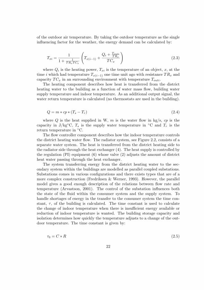
The flow controller component describes how the indoor temperature controlsthe district heating water flow. The radiator system, see Figure 2.2, consists of aseparate water system. The heat is transferred from the district heating side tothe radiator side through the heat exchanger (4). The heat supply is controlled bythe regulation (PI) equipment (6) whose valve (2) adjusts the amount of districtheat water passing through the heat exchanger.

The system transferring energy from the district heating water to the sec-ondary system within the buildings are modelled as parallel coupled substations.Substations comes in various configurations and there exists types that are of amore complex construction (Fredriksen & Werner, 1993). However, the parallelmodel gives a good enough description of the relations between flow rate andtemperature (Arvastson, 2001). The control of the substation influences boththe state of the fluid within the consumer system and the supply system. Tohandle shortages of energy in the transfer to the consumer system the time con-stant, τ , of the building is calculated. The time constant is used to calculatethe change of indoor temperature when there is insufficient energy available orreduction of indoor temperature is wanted. The building storage capacity andisolation determines how quickly the temperature adjusts to a change of the out-door temperature. The time constant is given by:

τ0 = C ∗R (2.5)

22

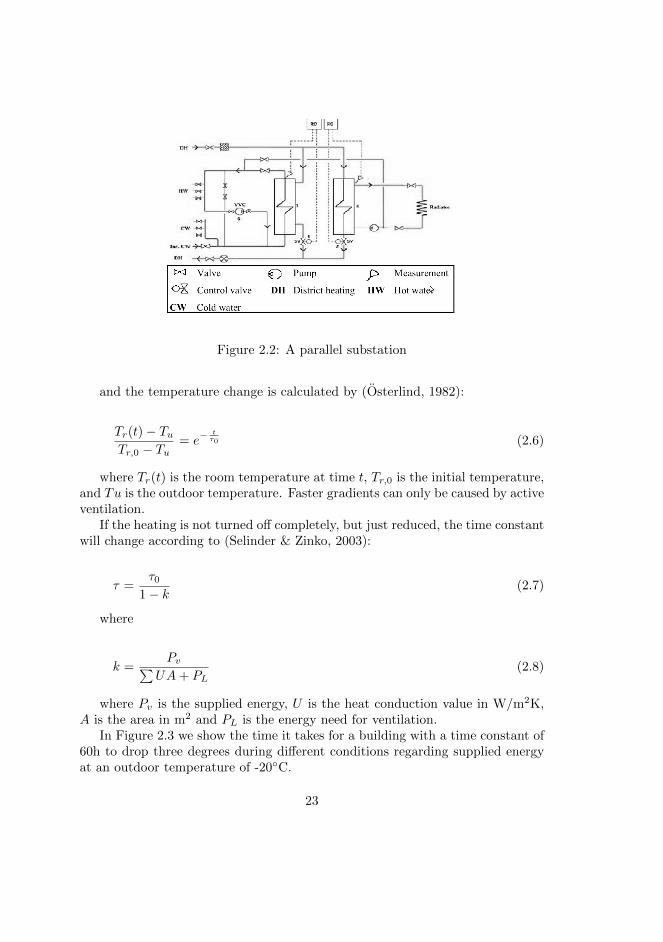
Figure 2.2: A parallel substation

and the temperature change is calculated by (Osterlind, 1982):

Tr(t)− TuTr,0 − Tu

= e−tτ0 (2.6)

where Tr(t) is the room temperature at time t, Tr,0 is the initial temperature,and Tu is the outdoor temperature. Faster gradients can only be caused by activeventilation.

If the heating is not turned off completely, but just reduced, the time constantwill change according to (Selinder & Zinko, 2003):

τ =τ0

1− k(2.7)

where

k =Pv∑

UA+ PL(2.8)

where Pv is the supplied energy, U is the heat conduction value in W/m2K,A is the area in m2 and PL is the energy need for ventilation.

In Figure 2.3 we show the time it takes for a building with a time constant of60h to drop three degrees during different conditions regarding supplied energyat an outdoor temperature of -20◦C.

23

Figure 2.3: Indoor temperature change during three cases of energy supply, 0%,50% and 90% supply respectively

The tap water system can be designed in different ways depending on thedemand. The system normally contains a circulation pump that circulate thewater at a low speed, this is done to minimize the bacterial content and to get arapid supply of hot water. Opposite to the radiator system, the tap water systemhas a dynamic valve set-up, i.e. the flow primarily depends on social factors.

The domestic hot tap water demand of the customers is simulated through atap water model (Arvastsson & Wollerstrand, 1997) where flow size and tappingdurability is determined by the simulation of a random number, Y , from a certaindistribution with cumulative distribution function FY , which can be performedusing uniformly distributed numbers, and where the time between tapping is anon-homogeneous Poisson process:

X = 1− exp

(−∫ T

0

µ(u)du

)(2.9)

where µ(u) is the time-varying opening intensity and T the time to derive.The opening intensities are derived from:

µ =p

(1− p)η(2.10)

where eta is given by measurement data (Holmberg, 1981) and µ is calculatedfrom the distribution function for open valve time. The probabilities for usageof hot tap water during the day is divided between Bath, Wash and Kitchenaccording to Figure 2.4.

24

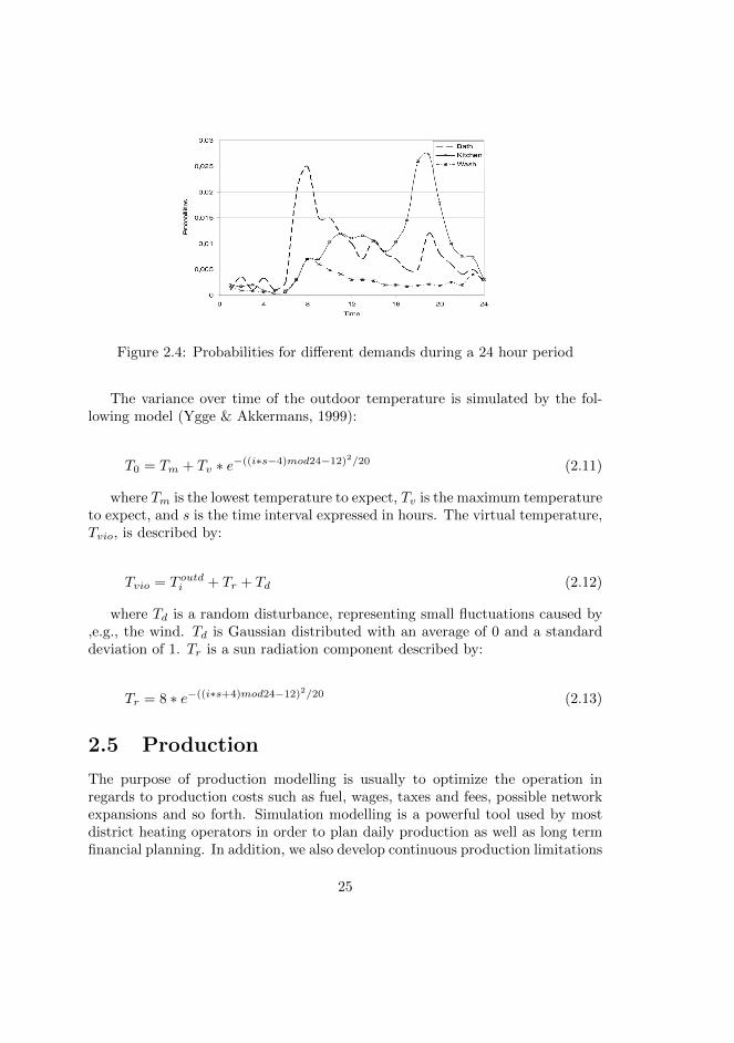
Figure 2.4: Probabilities for different demands during a 24 hour period

The variance over time of the outdoor temperature is simulated by the fol-lowing model (Ygge & Akkermans, 1999):

T0 = Tm + Tv ∗ e−((i∗s−4)mod24−12)2/20 (2.11)

where Tm is the lowest temperature to expect, Tv is the maximum temperatureto expect, and s is the time interval expressed in hours. The virtual temperature,Tvio, is described by:

Tvio = T outdi + Tr + Td (2.12)

where Td is a random disturbance, representing small fluctuations caused by,e.g., the wind. Td is Gaussian distributed with an average of 0 and a standarddeviation of 1. Tr is a sun radiation component described by:

Tr = 8 ∗ e−((i∗s+4)mod24−12)2/20 (2.13)

2.5 Production

The purpose of production modelling is usually to optimize the operation inregards to production costs such as fuel, wages, taxes and fees, possible networkexpansions and so forth. Simulation modelling is a powerful tool used by mostdistrict heating operators in order to plan daily production as well as long termfinancial planning. In addition, we also develop continuous production limitations

25

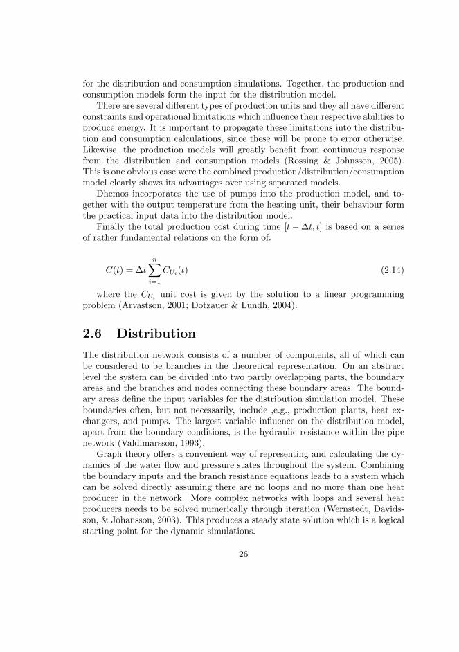
for the distribution and consumption simulations. Together, the production andconsumption models form the input for the distribution model.

There are several different types of production units and they all have differentconstraints and operational limitations which influence their respective abilities toproduce energy. It is important to propagate these limitations into the distribu-tion and consumption calculations, since these will be prone to error otherwise.Likewise, the production models will greatly benefit from continuous responsefrom the distribution and consumption models (Rossing & Johnsson, 2005).This is one obvious case were the combined production/distribution/consumptionmodel clearly shows its advantages over using separated models.

Dhemos incorporates the use of pumps into the production model, and to-gether with the output temperature from the heating unit, their behaviour formthe practical input data into the distribution model.

Finally the total production cost during time [t−∆t, t] is based on a seriesof rather fundamental relations on the form of:

C(t) = ∆t

n∑i=1

CUi(t) (2.14)

where the CUi unit cost is given by the solution to a linear programmingproblem (Arvastson, 2001; Dotzauer & Lundh, 2004).

2.6 Distribution

The distribution network consists of a number of components, all of which canbe considered to be branches in the theoretical representation. On an abstractlevel the system can be divided into two partly overlapping parts, the boundaryareas and the branches and nodes connecting these boundary areas. The bound-ary areas define the input variables for the distribution simulation model. Theseboundaries often, but not necessarily, include ,e.g., production plants, heat ex-changers, and pumps. The largest variable influence on the distribution model,apart from the boundary conditions, is the hydraulic resistance within the pipenetwork (Valdimarsson, 1993).

Graph theory offers a convenient way of representing and calculating the dy-namics of the water flow and pressure states throughout the system. Combiningthe boundary inputs and the branch resistance equations leads to a system whichcan be solved directly assuming there are no loops and no more than one heatproducer in the network. More complex networks with loops and several heatproducers needs to be solved numerically through iteration (Wernstedt, Davids-son, & Johansson, 2003). This produces a steady state solution which is a logicalstarting point for the dynamic simulations.

26

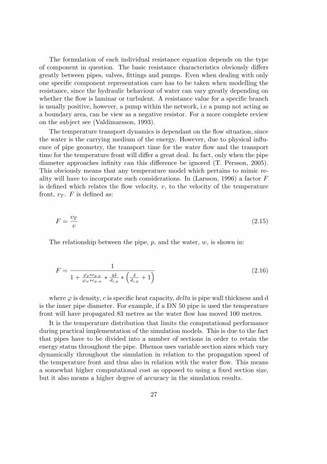
The formulation of each individual resistance equation depends on the typeof component in question. The basic resistance characteristics obviously differsgreatly between pipes, valves, fittings and pumps. Even when dealing with onlyone specific component representation care has to be taken when modelling theresistance, since the hydraulic behaviour of water can vary greatly depending onwhether the flow is laminar or turbulent. A resistance value for a specific branchis usually positive, however, a pump within the network, i.e a pump not acting asa boundary area, can be view as a negative resistor. For a more complete reviewon the subject see (Valdimarsson, 1993).

The temperature transport dynamics is dependant on the flow situation, sincethe water is the carrying medium of the energy. However, due to physical influ-ence of pipe geometry, the transport time for the water flow and the transporttime for the temperature front will differ a great deal. In fact, only when the pipediameter approaches infinity can this difference be ignored (T. Persson, 2005).This obviously means that any temperature model which pertains to mimic re-ality will have to incorporate such considerations. In (Larsson, 1996) a factor Fis defined which relates the flow velocity, v, to the velocity of the temperaturefront, vT . F is defined as:

F =vTv

(2.15)

The relationship between the pipe, p, and the water, w, is shown in:

F =1

1 +ϕp∗cp,pϕw∗cp,w ∗

4δdi,p∗(

δdi,p

+ 1) (2.16)

where ϕ is density, c is specific heat capacity, delta is pipe wall thickness and dis the inner pipe diameter. For example, if a DN 50 pipe is used the temperaturefront will have propagated 83 metres as the water flow has moved 100 metres.

It is the temperature distribution that limits the computational performanceduring practical implementation of the simulation models. This is due to the factthat pipes have to be divided into a number of sections in order to retain theenergy status throughout the pipe. Dhemos uses variable section sizes which varydynamically throughout the simulation in relation to the propagation speed ofthe temperature front and thus also in relation with the water flow. This meansa somewhat higher computational cost as opposed to using a fixed section size,but it also means a higher degree of accuracy in the simulation results.

27

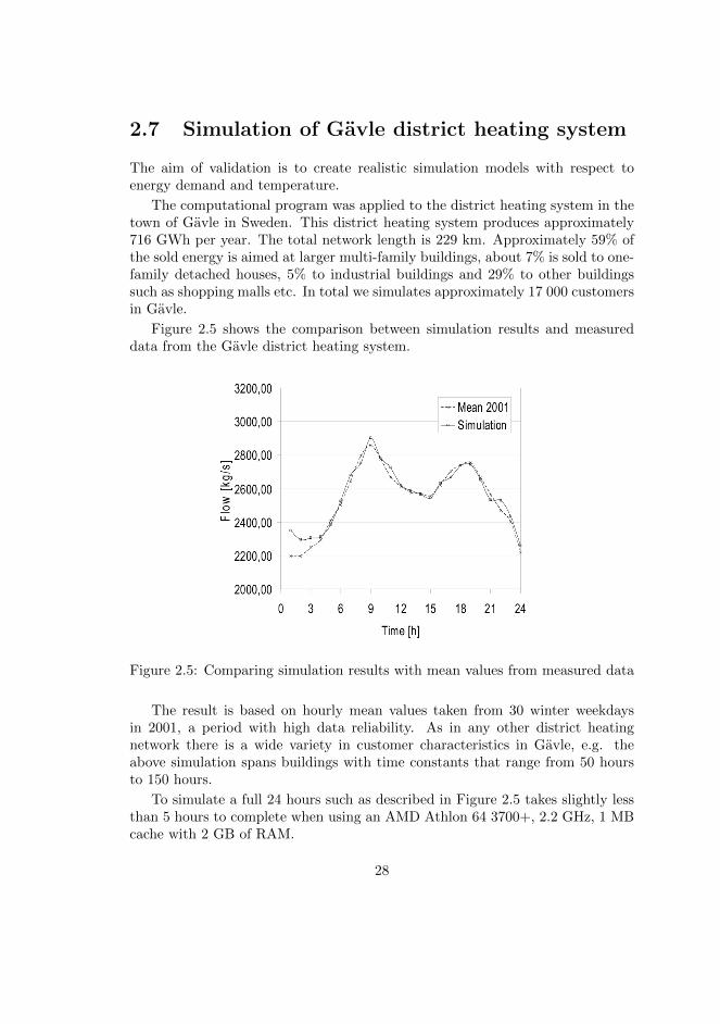
2.7 Simulation of Gavle district heating system

The aim of validation is to create realistic simulation models with respect toenergy demand and temperature.

The computational program was applied to the district heating system in thetown of Gavle in Sweden. This district heating system produces approximately716 GWh per year. The total network length is 229 km. Approximately 59% ofthe sold energy is aimed at larger multi-family buildings, about 7% is sold to one-family detached houses, 5% to industrial buildings and 29% to other buildingssuch as shopping malls etc. In total we simulates approximately 17 000 customersin Gavle.

Figure 2.5 shows the comparison between simulation results and measureddata from the Gavle district heating system.

Figure 2.5: Comparing simulation results with mean values from measured data

The result is based on hourly mean values taken from 30 winter weekdaysin 2001, a period with high data reliability. As in any other district heatingnetwork there is a wide variety in customer characteristics in Gavle, e.g. theabove simulation spans buildings with time constants that range from 50 hoursto 150 hours.

To simulate a full 24 hours such as described in Figure 2.5 takes slightly lessthan 5 hours to complete when using an AMD Athlon 64 3700+, 2.2 GHz, 1 MBcache with 2 GB of RAM.

28

2.8 Conclusions and future work

The practical importance of the simulator is not only for design of distributingnetworks, but in the operation of district heating systems. The possibility tosimulate the dynamic relations for various operating conditions is very useful fordispatchers in power and heating plants. This is a valuable contribution not onlyfrom a technical stand, but also from a financial viewpoint.

Dhemos has been compared with calculations made using MATLAB in orderto verify the various implementation solutions. After the analysis of the resultfrom the Gavle simulation we have found that Dhemos is reliable.

The distribution model uses a microscopic model which gives the ability tosimulate the behaviour of single endpoints within the network, which is necessarywhen studying the comfort fluctuations experienced by individual customers.

One problem with existing theoretical models is that they neglect the factthat a large population of the customer installations are working well belowtheir original capabilities. Dhemos implements short-circuits within the customersubstations in order to be able to simulate such deterioration in heat exchangerperformance.

Future work includes developing the presentational software in order to maxi-mize the usability of the system, e.g. operational pressure diagrams and so forth.We also plan to develop an interface between Dhemos and a general optimiza-tion engine in order to further optimize the capabilities of the system. The moretheoretical future work includes developing models for using genetic algorithmswithin Dhemos in order to find optimized solutions when expanding existing dis-trict heating networks. Also we need to expand the tap water models to includesuch buildings as single-family houses, industrial buildings, shopping malls andso forth.

29

30

Chapter 3

Paper II - Demand sidemanagement in districtheating systems

This paper describes a multi agent system that has made the voyage from researchproject to commercialised product. The purpose for the multi agent system isto dynamically control a system so that the load of the system is below certainthreshold values without reduction of quality of service and by that, to avoid theusage of top load production sources and to reduce energy consumption. Thefundamental idea behind the system is that a large number of small local decisionstaken all in all have great impact on the overall system performance. A field-testas well as a return of investment analysis are presented.

3.1 Keywords

Management, Performance, Economics, Reliability, Agent-based deployed appli-cations

3.2 Introduction

This paper describes a multi agent system that dynamically controls DistrictHeating Systems (DHS) so that the load of the system is kept below certainthreshold values without reducing of quality of service provided to the customers.The purpose is to avoid the usage of top load production sources (which often uses

31

fossil fuel) and to reduce energy consumption. The fundamental idea behind thesystem is that a large number of small local decisions together have great impacton the overall system performance.

This venture started as a research project in 1999 as a collaboration effortbetween Cetetherm (now Alfa Laval), and Blekinge Institute of Technology. Theproject has since evolved throughout the last few years into this current com-mercial project, an effort within which the spin-off company NODA IntelligentSystems AB was founded in early 2005. A field-test has just been completed andis reported in section 3.5. The main focus was to validate the system from atechnical standpoint. However, since our intent is to commercialise the system,the economical benefits were equally important to investigate.

3.2.1 Background

The basic idea behind district heating is to use local heat production plantsto produce hot water. This water is then distributed by using one or morepumps at approximately 1-3 m/s through pipes to the customers where HeatExchange Systems (HES) are used to exchange heat from the primary flow ofthe distribution pipes to the secondary flows of the building. The secondaryflows are used for heating both tap water and the building itself. In large citiesdistrict heating networks tend to be very complex, including tens of thousandsof substations and hundreds of kilometres of distribution pipes with distributiontimes up to 24 hours.

The energy load of any DHS is subject to large variations due to the fluc-tuating demands of customers. The energy load is mainly divided between therather slow process of space heating and the fast process of domestic hot tap wa-ter consumption. A DHS must be capable of meeting all such fluctuating energydemands.

Optimisation of DHS has traditionally focused on production plants and dis-tribution systems. However, in the last ten years, consumer heating systems(HES) have received increased attention. The product development of HES haschanged from focusing on the component (sub optimisation) to focusing on theinteraction of the components (system optimisation) (Andersen & Poulsen, 1999).HES, as the heat load source of a DHS, determine the operation of the total DHS.Yet it is unusual that the operation of HES can be monitored or controlled bythe DHS operator. The operation strategies of the DHS are therefore limited toproviding sufficiently high temperature and pressure to all customers, withoutany possibility of actually optimising the system as a whole.

Load control HES can either be achieved directly by remote control of in-dividual HES or indirectly by usage of various tariffs. Indirect load control iswidely used and has primarily been implemented by the usage of flow tariffs,

32

i.e., customers are charged according to the flow in comparison to a referencevalue for the flow. Direct load control is very uncommon but there exists a fewattempts, e.g., a centralised load control system that was studied by Osterlind(Osterlind, 1982). Osterlind used a one-way communication link on the electric-ity network to manipulate the outdoor temperature meters of individual HES. Bythis communication link he was able to manipulate and control the space heatingof the connected buildings. The study confirmed earlier theories of centralisedload control and showed that it is relatively easy to achieve robustness againstshortage situations in DHS. However, the system did not consider, e.g., fairnessand the quality of service (QoS) delivered to the individual consumer. Oster-lind also concluded that two-way communication was a minimum requirementfor an operational system (Osterlind, 1990). Two-way communication systemsfor DH substations are currently at a relatively early stage of development. How-ever, as hardware is becoming available focus should now be on how to use thedata/information and how to achieve savings (Drysdale & Stang, 2002).

Energy is not an end in itself; instead it is a means to provide a numberof services. Businesses and households view energy as an input, an expense ofdoing business or maintaining a home. They are less concerned with how manykilowatt hours they purchase than with the services that the energy provides, e.g.,space heating. This relationship provides the basis of demand-side management(DSM). DSM can be defined as

”The planning and implementation of strategies designed to encourageconsumers to improve energy efficiency, reduce energy costs, changethe time of usage or promote the use of a different energy source”(LIPAedge, 2005)

. DSM strategies try to reduce the peak load and change the shape of the loadprofile through the techniques of peak clipping, load shifting and energy conser-vation. DSM activities should bring the demand and supply closer to a perceivedoptimum. Correctly implemented, DSM strategies can reduce energy consump-tion with the associated financial and environmental benefits. The idea behindenergy efficiency is quite simple; if people consume less energy, there will be lessemission of greenhouse gases as the result of less burning of fossil fuels in heatproduction plants. Energy efficiency technologies and practices can therefore playa significant role in reducing the threat of global climate change.

There is very little information and expertise available on DSM for DHS. To-day, there is a growing interest, but while DSM has become a standard techniquefor the electricity market (Levin & Wesslen, 1993; Johansson & Ejeklint, 1991;Aune, 2001; Nordvik & Lund, 2003; P. Johansson, 2003), it is still in the earlystages when considering DHS (Heating & Cooling, 2002). The goal of DSM isto be able to control the heat load at an overall system level rather than to

33

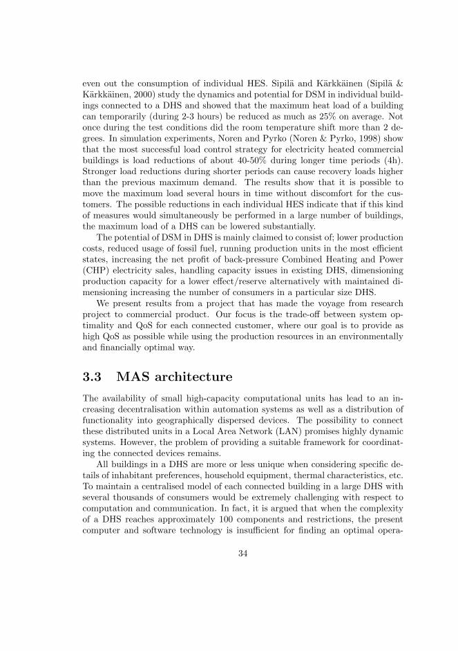
even out the consumption of individual HES. Sipila and Karkkainen (Sipila &Karkkainen, 2000) study the dynamics and potential for DSM in individual build-ings connected to a DHS and showed that the maximum heat load of a buildingcan temporarily (during 2-3 hours) be reduced as much as 25% on average. Notonce during the test conditions did the room temperature shift more than 2 de-grees. In simulation experiments, Noren and Pyrko (Noren & Pyrko, 1998) showthat the most successful load control strategy for electricity heated commercialbuildings is load reductions of about 40-50% during longer time periods (4h).Stronger load reductions during shorter periods can cause recovery loads higherthan the previous maximum demand. The results show that it is possible tomove the maximum load several hours in time without discomfort for the cus-tomers. The possible reductions in each individual HES indicate that if this kindof measures would simultaneously be performed in a large number of buildings,the maximum load of a DHS can be lowered substantially.

The potential of DSM in DHS is mainly claimed to consist of; lower productioncosts, reduced usage of fossil fuel, running production units in the most efficientstates, increasing the net profit of back-pressure Combined Heating and Power(CHP) electricity sales, handling capacity issues in existing DHS, dimensioningproduction capacity for a lower effect/reserve alternatively with maintained di-mensioning increasing the number of consumers in a particular size DHS.

We present results from a project that has made the voyage from researchproject to commercial product. Our focus is the trade-off between system op-timality and QoS for each connected customer, where our goal is to provide ashigh QoS as possible while using the production resources in an environmentallyand financially optimal way.

3.3 MAS architecture

The availability of small high-capacity computational units has lead to an in-creasing decentralisation within automation systems as well as a distribution offunctionality into geographically dispersed devices. The possibility to connectthese distributed units in a Local Area Network (LAN) promises highly dynamicsystems. However, the problem of providing a suitable framework for coordinat-ing the connected devices remains.

All buildings in a DHS are more or less unique when considering specific de-tails of inhabitant preferences, household equipment, thermal characteristics, etc.To maintain a centralised model of each connected building in a large DHS withseveral thousands of consumers would be extremely challenging with respect tocomputation and communication. In fact, it is argued that when the complexityof a DHS reaches approximately 100 components and restrictions, the presentcomputer and software technology is insufficient for finding an optimal opera-

34

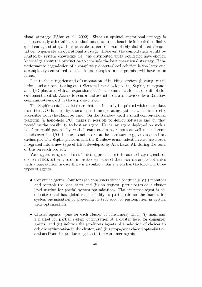
tional strategy (Bohm et al., 2002). Since an optimal operational strategy isnot practically achievable, a method based on some heuristic is needed to find agood-enough strategy. It is possible to perform completely distributed compu-tation to generate an operational strategy. However, the computation would belimited by system knowledge, i.e., the distributed units would not have enoughknowledge about the production to conclude the best operational strategy. If theperformance degradation of a completely decentralised solution is too large anda completely centralised solution is too complex, a compromise will have to befound.

Due to the rising demand of automation of building services (heating, venti-lation, and air-conditioning etc.) Siemens have developed the Saphir, an expand-able I/O platform with an expansion slot for a communication card, suitable forequipment control. Access to sensor and actuator data is provided by a Rainbowcommunication card in the expansion slot.

The Saphir contains a database that continuously is updated with sensor datafrom the I/O channels by a small real-time operating system, which is directlyaccessible from the Rainbow card. On the Rainbow card a small computationalplatform (a hand-held PC) makes it possible to deploy software and by thatproviding the possibility to host an agent. Hence, an agent deployed on such aplatform could potentially read all connected sensor input as well as send com-mands over the I/O channel to actuators on the hardware, e.g., valves on a heatexchanger. The Saphir platform and the Rainbow communication card have beenintegrated into a new type of HES, developed by Alfa Laval AB during the termof this research project.

We suggest using a semi-distributed approach. In this case each agent, embed-ded on a HES, is trying to optimise its own usage of the resources and coordinateswith a base station in case there is a conflict. Our system has the following threetypes of agents:

� Consumer agents: (one for each consumer) which continuously (i) monitorsand controls the local state and (ii) on request, participates on a clusterlevel market for partial system optimisation. The consumer agent is co-operative and has global responsibility to participate on the market forsystem optimisation by providing its true cost for participation in systemwide optimisation.

� Cluster agents: (one for each cluster of consumers) which (i) maintainsa market for partial system optimisation at a cluster level for consumeragents, and (ii) informs the producers agents of a selection of choices toachieve optimisation in the cluster, and (iii) propagates chosen optimisationactions from the producer agents to the consumer agents.

35

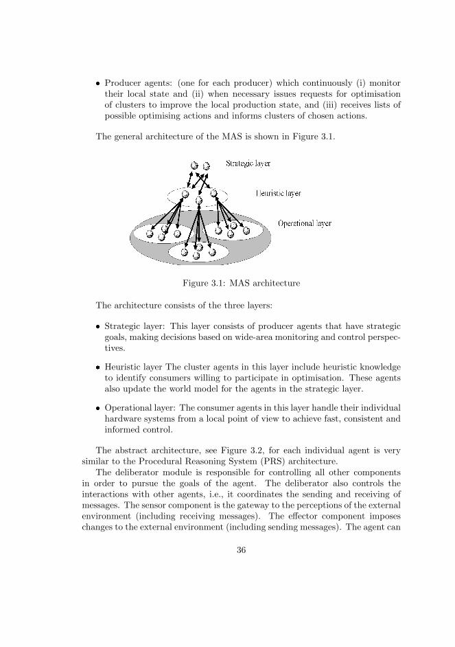
� Producer agents: (one for each producer) which continuously (i) monitortheir local state and (ii) when necessary issues requests for optimisationof clusters to improve the local production state, and (iii) receives lists ofpossible optimising actions and informs clusters of chosen actions.

The general architecture of the MAS is shown in Figure 3.1.

Figure 3.1: MAS architecture

The architecture consists of the three layers:

� Strategic layer: This layer consists of producer agents that have strategicgoals, making decisions based on wide-area monitoring and control perspec-tives.

� Heuristic layer The cluster agents in this layer include heuristic knowledgeto identify consumers willing to participate in optimisation. These agentsalso update the world model for the agents in the strategic layer.

� Operational layer: The consumer agents in this layer handle their individualhardware systems from a local point of view to achieve fast, consistent andinformed control.

The abstract architecture, see Figure 3.2, for each individual agent is verysimilar to the Procedural Reasoning System (PRS) architecture.

The deliberator module is responsible for controlling all other componentsin order to pursue the goals of the agent. The deliberator also controls theinteractions with other agents, i.e., it coordinates the sending and receiving ofmessages. The sensor component is the gateway to the perceptions of the externalenvironment (including receiving messages). The effector component imposeschanges to the external environment (including sending messages). The agent can

36

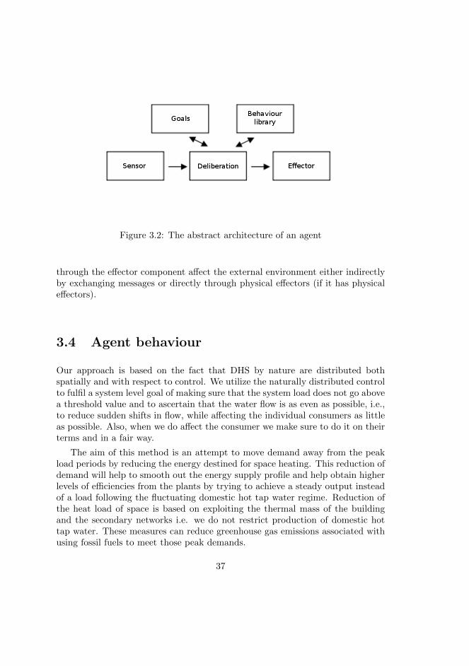
Figure 3.2: The abstract architecture of an agent

through the effector component affect the external environment either indirectlyby exchanging messages or directly through physical effectors (if it has physicaleffectors).

3.4 Agent behaviour

Our approach is based on the fact that DHS by nature are distributed bothspatially and with respect to control. We utilize the naturally distributed controlto fulfil a system level goal of making sure that the system load does not go abovea threshold value and to ascertain that the water flow is as even as possible, i.e.,to reduce sudden shifts in flow, while affecting the individual consumers as littleas possible. Also, when we do affect the consumer we make sure to do it on theirterms and in a fair way.

The aim of this method is an attempt to move demand away from the peakload periods by reducing the energy destined for space heating. This reduction ofdemand will help to smooth out the energy supply profile and help obtain higherlevels of efficiencies from the plants by trying to achieve a steady output insteadof a load following the fluctuating domestic hot tap water regime. Reduction ofthe heat load of space is based on exploiting the thermal mass of the buildingand the secondary networks i.e. we do not restrict production of domestic hottap water. These measures can reduce greenhouse gas emissions associated withusing fossil fuels to meet those peak demands.

37

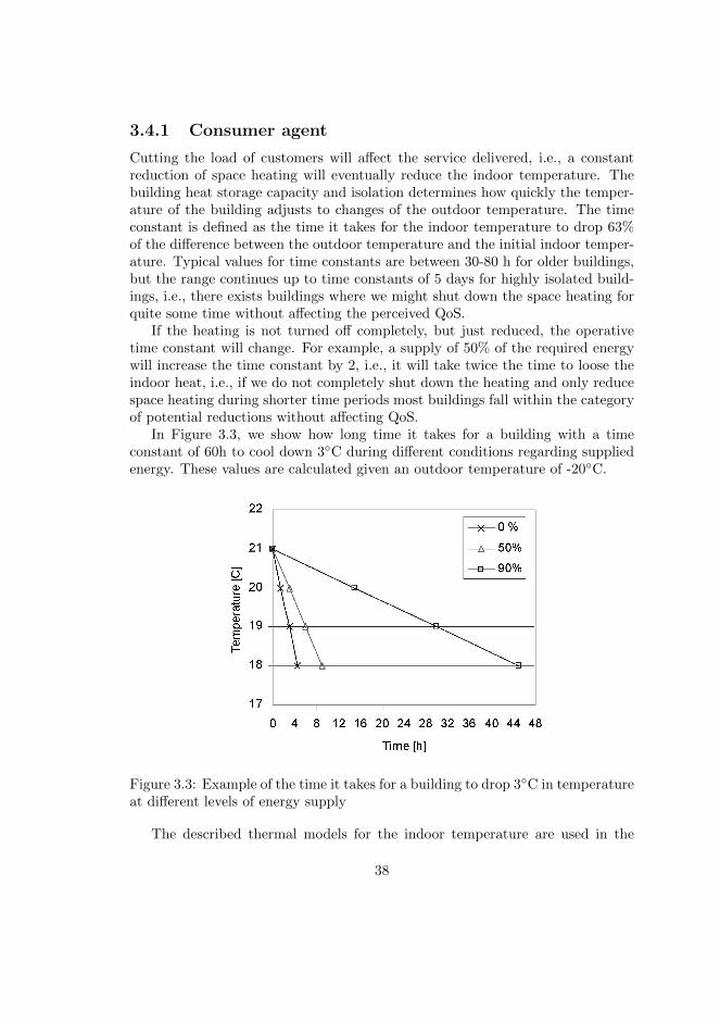
3.4.1 Consumer agent

Cutting the load of customers will affect the service delivered, i.e., a constantreduction of space heating will eventually reduce the indoor temperature. Thebuilding heat storage capacity and isolation determines how quickly the temper-ature of the building adjusts to changes of the outdoor temperature. The timeconstant is defined as the time it takes for the indoor temperature to drop 63%of the difference between the outdoor temperature and the initial indoor temper-ature. Typical values for time constants are between 30-80 h for older buildings,but the range continues up to time constants of 5 days for highly isolated build-ings, i.e., there exists buildings where we might shut down the space heating forquite some time without affecting the perceived QoS.

If the heating is not turned off completely, but just reduced, the operativetime constant will change. For example, a supply of 50% of the required energywill increase the time constant by 2, i.e., it will take twice the time to loose theindoor heat, i.e., if we do not completely shut down the heating and only reducespace heating during shorter time periods most buildings fall within the categoryof potential reductions without affecting QoS.

In Figure 3.3, we show how long time it takes for a building with a timeconstant of 60h to cool down 3◦C during different conditions regarding suppliedenergy. These values are calculated given an outdoor temperature of -20◦C.

Figure 3.3: Example of the time it takes for a building to drop 3◦C in temperatureat different levels of energy supply

The described thermal models for the indoor temperature are used in the

38

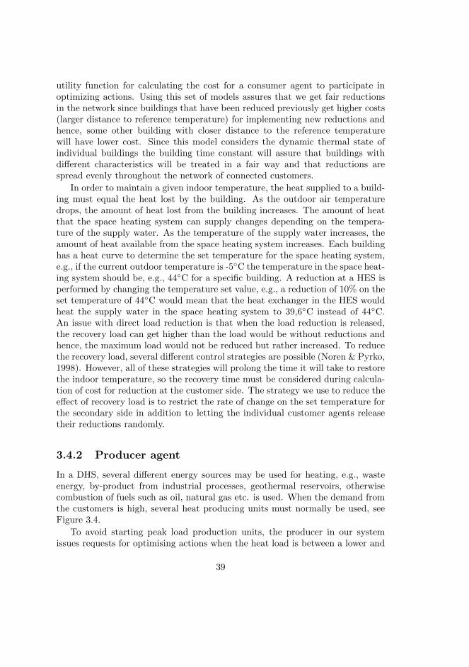
utility function for calculating the cost for a consumer agent to participate inoptimizing actions. Using this set of models assures that we get fair reductionsin the network since buildings that have been reduced previously get higher costs(larger distance to reference temperature) for implementing new reductions andhence, some other building with closer distance to the reference temperaturewill have lower cost. Since this model considers the dynamic thermal state ofindividual buildings the building time constant will assure that buildings withdifferent characteristics will be treated in a fair way and that reductions arespread evenly throughout the network of connected customers.

In order to maintain a given indoor temperature, the heat supplied to a build-ing must equal the heat lost by the building. As the outdoor air temperaturedrops, the amount of heat lost from the building increases. The amount of heatthat the space heating system can supply changes depending on the tempera-ture of the supply water. As the temperature of the supply water increases, theamount of heat available from the space heating system increases. Each buildinghas a heat curve to determine the set temperature for the space heating system,e.g., if the current outdoor temperature is -5◦C the temperature in the space heat-ing system should be, e.g., 44◦C for a specific building. A reduction at a HES isperformed by changing the temperature set value, e.g., a reduction of 10% on theset temperature of 44◦C would mean that the heat exchanger in the HES wouldheat the supply water in the space heating system to 39,6◦C instead of 44◦C.An issue with direct load reduction is that when the load reduction is released,the recovery load can get higher than the load would be without reductions andhence, the maximum load would not be reduced but rather increased. To reducethe recovery load, several different control strategies are possible (Noren & Pyrko,1998). However, all of these strategies will prolong the time it will take to restorethe indoor temperature, so the recovery time must be considered during calcula-tion of cost for reduction at the customer side. The strategy we use to reduce theeffect of recovery load is to restrict the rate of change on the set temperature forthe secondary side in addition to letting the individual customer agents releasetheir reductions randomly.

3.4.2 Producer agent

In a DHS, several different energy sources may be used for heating, e.g., wasteenergy, by-product from industrial processes, geothermal reservoirs, otherwisecombustion of fuels such as oil, natural gas etc. is used. When the demand fromthe customers is high, several heat producing units must normally be used, seeFigure 3.4.

To avoid starting peak load production units, the producer in our systemissues requests for optimising actions when the heat load is between a lower and

39

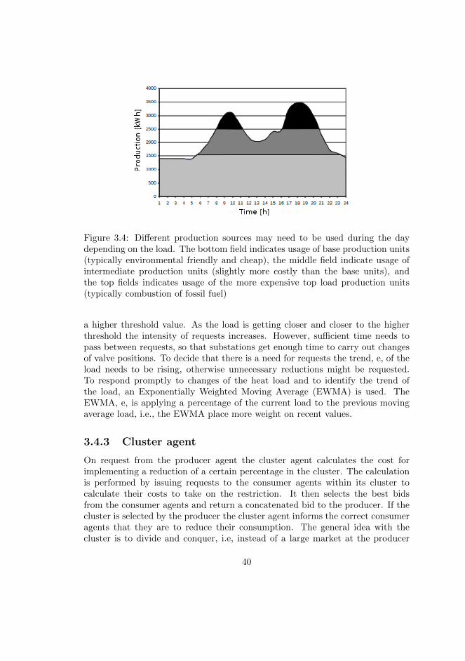
Figure 3.4: Different production sources may need to be used during the daydepending on the load. The bottom field indicates usage of base production units(typically environmental friendly and cheap), the middle field indicate usage ofintermediate production units (slightly more costly than the base units), andthe top fields indicates usage of the more expensive top load production units(typically combustion of fossil fuel)

a higher threshold value. As the load is getting closer and closer to the higherthreshold the intensity of requests increases. However, sufficient time needs topass between requests, so that substations get enough time to carry out changesof valve positions. To decide that there is a need for requests the trend, e, of theload needs to be rising, otherwise unnecessary reductions might be requested.To respond promptly to changes of the heat load and to identify the trend ofthe load, an Exponentially Weighted Moving Average (EWMA) is used. TheEWMA, e, is applying a percentage of the current load to the previous movingaverage load, i.e., the EWMA place more weight on recent values.

3.4.3 Cluster agent

On request from the producer agent the cluster agent calculates the cost forimplementing a reduction of a certain percentage in the cluster. The calculationis performed by issuing requests to the consumer agents within its cluster tocalculate their costs to take on the restriction. It then selects the best bidsfrom the consumer agents and return a concatenated bid to the producer. If thecluster is selected by the producer the cluster agent informs the correct consumeragents that they are to reduce their consumption. The general idea with thecluster is to divide and conquer, i.e, instead of a large market at the producer

40

we use a number of smaller markets. In this way we maintain local information,e.g., which agents populates a certain area, and makes the problem of choosingsubstations easier for the producer. The cluster agent is also responsible to makesure that restrictions are implemented, e.g., if the environment for a consumeragent (that is supposed to take on a restriction) changes beyond the model of theconsumer agent. The cluster agent needs to find another agent within its clusterto take on the restriction. If it fails to find another consumer agent, it informs theproducer that the restriction failed. Finally, another task for the cluster agent isto estimate the current consumption within the cluster and inform the producerof this at regular intervals.

3.5 Deployed system

The area where the agent system is installed is composed of 14 buildings witha total of 350 apartments. The district heating network for the area is veryfavourable since it can be seen as a separate part of the network in the town,see Figure 3.5. We were thus able to monitor the total delivered energy to thearea for verification purposes. To monitor the energy delivered to the area weinstalled a clamp-on flow meter on the pipe at the entrance to the area, close tothe PC building.

Figure 3.5: Connected buildings

41

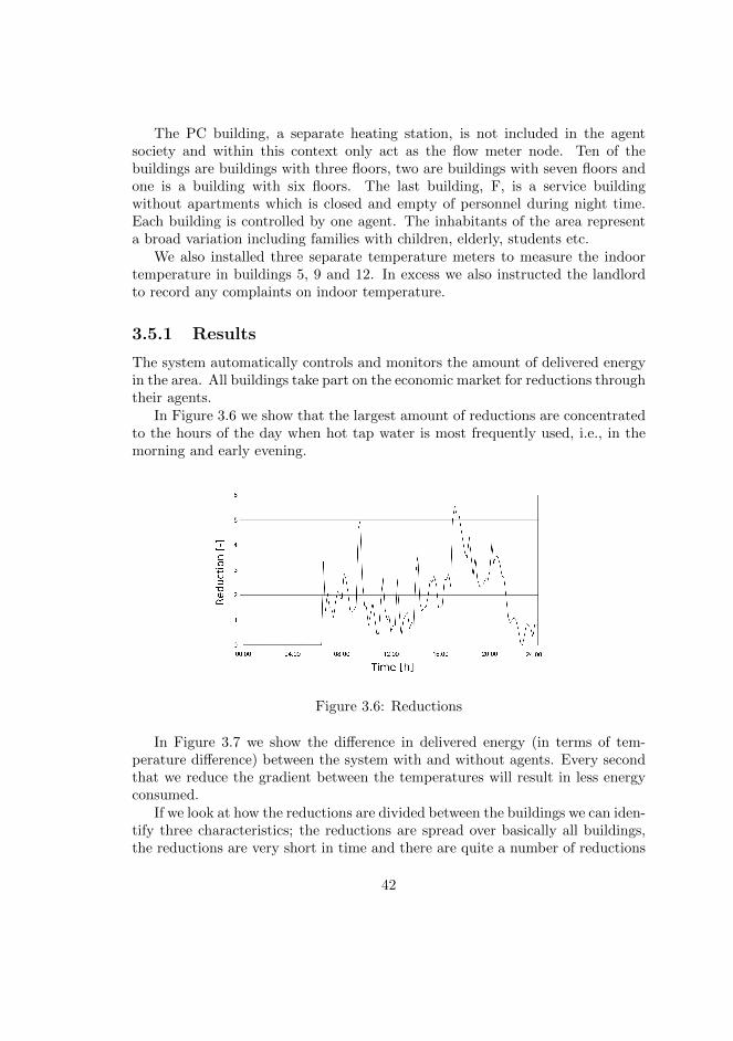
The PC building, a separate heating station, is not included in the agentsociety and within this context only act as the flow meter node. Ten of thebuildings are buildings with three floors, two are buildings with seven floors andone is a building with six floors. The last building, F, is a service buildingwithout apartments which is closed and empty of personnel during night time.Each building is controlled by one agent. The inhabitants of the area representa broad variation including families with children, elderly, students etc.

We also installed three separate temperature meters to measure the indoortemperature in buildings 5, 9 and 12. In excess we also instructed the landlordto record any complaints on indoor temperature.

3.5.1 Results

The system automatically controls and monitors the amount of delivered energyin the area. All buildings take part on the economic market for reductions throughtheir agents.

In Figure 3.6 we show that the largest amount of reductions are concentratedto the hours of the day when hot tap water is most frequently used, i.e., in themorning and early evening.

Figure 3.6: Reductions

In Figure 3.7 we show the difference in delivered energy (in terms of tem-perature difference) between the system with and without agents. Every secondthat we reduce the gradient between the temperatures will result in less energyconsumed.

If we look at how the reductions are divided between the buildings we can iden-tify three characteristics; the reductions are spread over basically all buildings,the reductions are very short in time and there are quite a number of reductions

42

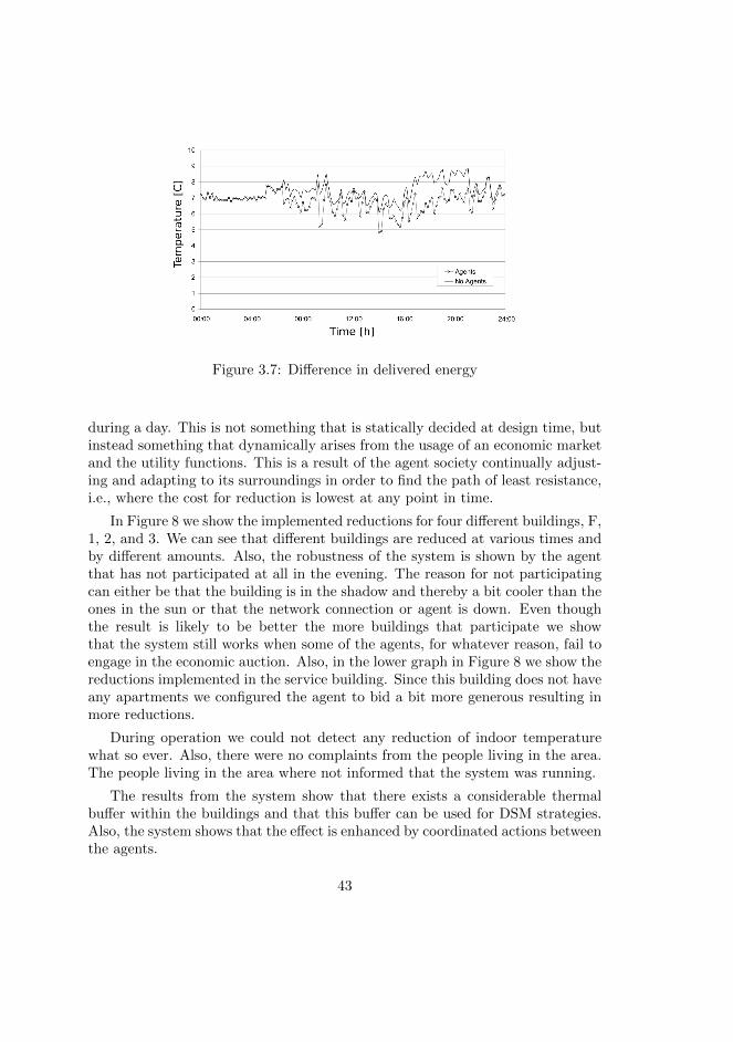
Figure 3.7: Difference in delivered energy

during a day. This is not something that is statically decided at design time, butinstead something that dynamically arises from the usage of an economic marketand the utility functions. This is a result of the agent society continually adjust-ing and adapting to its surroundings in order to find the path of least resistance,i.e., where the cost for reduction is lowest at any point in time.

In Figure 8 we show the implemented reductions for four different buildings, F,1, 2, and 3. We can see that different buildings are reduced at various times andby different amounts. Also, the robustness of the system is shown by the agentthat has not participated at all in the evening. The reason for not participatingcan either be that the building is in the shadow and thereby a bit cooler than theones in the sun or that the network connection or agent is down. Even thoughthe result is likely to be better the more buildings that participate we showthat the system still works when some of the agents, for whatever reason, fail toengage in the economic auction. Also, in the lower graph in Figure 8 we show thereductions implemented in the service building. Since this building does not haveany apartments we configured the agent to bid a bit more generous resulting inmore reductions.

During operation we could not detect any reduction of indoor temperaturewhat so ever. Also, there were no complaints from the people living in the area.The people living in the area where not informed that the system was running.

The results from the system show that there exists a considerable thermalbuffer within the buildings and that this buffer can be used for DSM strategies.Also, the system shows that the effect is enhanced by coordinated actions betweenthe agents.

43

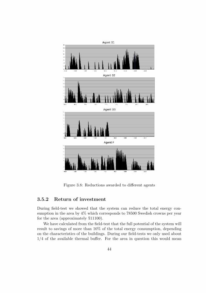
Figure 3.8: Reductions awarded to different agents

3.5.2 Return of investment

During field-test we showed that the system can reduce the total energy con-sumption in the area by 4% which corresponds to 78500 Swedish crowns per yearfor the area (approximately $11100).

We have calculated from the field-test that the full potential of the system willresult to savings of more than 10% of the total energy consumption, dependingon the characteristics of the buildings. During our field-tests we only used about1/4 of the available thermal buffer. For the area in question this would mean

44

savings of approximately 235000 Swedish crowns a year (approximately $33200).Given that the system only has to cover its own investment costs, since the HESnormally covers its own costs, the system gives full return of investment withinthe first year.

3.5.3 Discussion

The results from the field-tests show a clear profit for the estate owners, sincewe reduce the amount of energy consumed. At the same time we argue thatthe operators of the district heating systems will benefit from the system. Atfirst this might seem contradictory but there are several system wide benefitswith DSM which more than compensates the operators for the reduced energysale. For example, the flow balancing that we showed in the field-tests wouldin the long run offer the operators a possibility to handle flow and capacityproblems in different parts of the network. This is an important issue since muchof the core of today networks were built during the 60s and 70s without anypossibility to foresee the enormous expansion of many district heating systemsduring resent years. Another example is operators who have low availability ofbase load production and are forced to use fossil fuel as a production source forenergy during peak loads. There are obvious major economical and environmentalbenefits in reducing the use of these peak load burners.

3.6 Conclusions

A DHS without an overall control system is basically composed of a number ofcompletely selfish and autonomous units, i.e., substations, working only to satisfytheir own local goals (sufficient domestic hot tap water and indoor temperature)without any consideration whatsoever about the overall efficiency of the system orthe state of other units in the network. We have introduced a level of automaticsystem control by using a semi-distributed MAS architecture to show the valueof cooperation among HES in DHS. In this paper we have shown that the valueof a large number of small local decisions taken all in all has a great impact ofthe overall system performance. The system described in this paper does notconsider load moving, only load shedding, i.e. where the total energy deliveredis not the same with agents as without them.

However, the results in this paper indicate that it is possible to remove 10%of the heating load without affecting the QoS delivered. The results also indicatethat it is possible to extend the number of customers in an existing DHS withoutthe need of increasing the production capacity.

All DHS are more or less unique when considering specific details of inhabitantpreferences, household equipment, size etc. This, of course, complicate matters

45

when about to draw general conclusions from a single installation. However, wehave shown that there are clear benefits of DSM in DHS and that it is a viableapproach to address the over all system control with a MAS.

The principle of DSM works when the total system utility is more importantthan the individual, i.e., there is a need of partial global responsibility from thecustomers. This responsibility could be created both by economic incentives aswell as by environmental incentives. The picture is not clear whether customerswill accept reductions without economic compensation or not. In reports regard-ing the electricity market it has been stated that it is a necessity to compensatecustomers otherwise they will not participate (Energimyndigheten, 2002) andthat there in Sweden today is no incentive for individual customers to save en-ergy during peak load hours since tariffs are constant during the day (Osterman,2005). However, there are also reports indicating that customers are interestedin saving the planet for free as well (Pyrko, Sernhed, & J., 2005).

It is worth noting that the project has also given rise to a spin-off researchproject dealing with the intricacies of simulating the dynamics within a DHS(?, ?). It was necessary to develop this simulator in order to validate the DSMstrategy before it was applied in a real DHS with real customers and producers.

3.7 Future work

We will in future experiments focus on developing load-shifting strategies for theMAS, i.e., not only reducing the load but also moving the load in time. Wewill also perform studies on primary return temperatures to investigate if it ispossible to develop strategies for the MAS to reduce the return temperaturesthus facilitating an increased efficiency in the use of CHP production. Futurework also include studies on differential tariffs in DHS as well as investigations ofpossible approaches to a complete market-oriented approach to the managementof DHS where producers are competing and where there is third-party access.

Controlling the load has potentially major benefits to CHP production and itwould be interesting to connect the load controlling strategies to, e.g., the energyprices at Nord Pool (The Nordic Power Exchange).

3.8 Acknowledgements

This project has been supported by VINNOVA and was a collaboration betweenNODA Intelligent Systems AB, Blekinge Institute of Technology and Alfa Laval.The commercialising effort has been supported by Karlshamnsbostader, Karl-shamns Energi, Sparbanken i Karlshamn and Blekinge Business Incubator.

46

Chapter 4

Paper III - Intelligentdistributed load control

In this paper we present results from a field test where a distributed load controlsystem uses load shedding to even out the daily fluctuations normally found in theenergy demand within a district heating system. We also discuss the frameworkupon which this system is built. The results promise both economical and envi-ronmental benefits without compromising the delivered quality of service, as wellas a win-win situation for the district heating provider and the end customer.

4.1 Introduction

The energy load of any district heating system is subject to large variations dueto the fluctuating demands of customers. The energy load is mainly dividedbetween the rather slow process of space heating and the fast process of domestichot tap water production. A district heating system must be capable of meetingall such fluctuating energy demands. Although there are large variations in theheat load between summer and wintertime, there is still a value in evening outthese fluctuations. Heat exchanger systems, as the source of the heat load withina district heating system, determine the behaviour of the total district heatingsystem. Yet it is unusual that the operation of heat exchanger systems can beremotely monitored and controlled by the district heating system operator. Theoperation strategies of the district heating system are therefore basically limitedto providing sufficiently high temperature and pressure to all customers, withoutany possibility of actually optimizing the system as a whole.

The objective of demand side management and load control in energy systems

47

is typically defined as; to optimize the production and distribution of energyby manipulating the consumption. Traditionally demand side management isachieved indirectly e.g. by the use of various tariffs or by production basedsystems requesting the cooperation of consumer utilities. Load control, on theother hand, uses remote control in order to directly control the behaviour ofthe participating consumer systems. However, the distinction between demandside management and load control is becoming increasingly blurred as emergingdemand side management based technologies are incorporating direct load controlprinciples.

Basic indirect demand side management is widely used and has primarily beenimplemented by the usage of flow tariffs, i.e. customers are charged according tothe flow in comparison to a reference value for the flow. Sipila and Karkkainen(Sipila & Karkkainen, 2000) study the dynamics and potential for demand sidemanagement in individual buildings connected to a district heating system andshowed that the maximum heat load of a building can temporarily (during 2-3hours) be reduced as much as 25% on average. Not once during the test conditionsdid the room temperature shift more than two degrees.

Direct load control is very uncommon but there exists a few attempts, e.g. acentralised load control system that was studied by Osterlind (Osterlind, 1982)during the early nineteen eighties. Osterlind used a one-way communication linkon the electricity network to manipulate the outdoor temperature meters of in-dividual heat exchanger systems. By this communication link he was able tomanipulate and control the space heating of the connected buildings. The studyconfirmed earlier theories on centralized load control and indicated the relativeease with which one could achieve effective and robust protection against short-age situations in district heating systems. However, the system fell short whentaking into account a number of real world considerations, e.g. fairness withinthe process and the quality of service (QoS) delivered to the individual con-sumer. Osterlind also concluded that two-way communication was a minimumrequirement for an operational system, and that although the system seemed as apromising approach the available state-of-the-art technology was simply not suffi-cient. Heat exchanger systems supporting two-way communication and sufficientcomputational performance are still at a relatively early stage of development.However, as reliable hardware which offers a favourable price ratio is becomingmore widely available, it is high time to turn the focus on how to fully utilize theexisting possibilities. The system presented in the following sections build andexpands upon the ideas and concepts found in the work of Osterlind.

48

4.1.1 Demand side management quality filter

As sensors and communication devices are becoming more sophisticated, the over-laying control system promises the possibility to exercise a more precise control ofconsumer behaviour. This new possibility does, however, come with a price. Thesystem wide control system will need to adapt to a more dynamic, unpredictableand open domain. Shortened time windows for decisions and increasing num-bers of available sensors leads to vast amounts of data and information. Factorsthat we argue necessitate a higher degree of autonomy and decentralization. Theobjective is to achieve the goal of optimizing the production while continuouslyupholding the QoS delivered to each customer. These two goals may well be ina state of conflict, e.g. consider the problem of deciding when to initiate, andduring what interval to run, an expensive and environmentally unsound peakload boiler, without compromising the QoS. The core of the problem lies in com-bining adequate QoS consideration policies with the sometimes invasive controlstrategies of demand side management and load control which are nonethelessneeded to fulfil operational optimization requirements. In order to address thisissue and to form the basis for a future framework within intelligent demand sidemanagement and load control we propose the introduction of an intermediaryquality insurance filter which adds a layer of intelligence in order to negotiate thebalance and bridge the gap between these conflicting goals.

Since such a layer will act as a mediator within a dynamic and changeabledomain, we believe it will need to be robust, flexible and responsive. Also, as thecomplexity grows such a system will need to evolve towards a more distributedarchitecture, in order to maintain sufficient fault tolerance and computationalperformance. A distributed system consisting of independent and autonomousentities which coordinate and synchronize their behaviour while being self-awareabout their respective QoS constraints is ultimately needed in order to fulfil therequirements. The main methodology for modelling the interactions between suchautonomous entities are based on ideas found in economics and game theory.We believe that these ideas combined with the resource constraints and QoSconsiderations yield a powerful framework for system wide optimization withindistrict heating systems.

4.2 Demand side management quality filter fordistrict heating systems

We consider the QoS delivered to each customer as the most important constraintin this domain. To compromise this constraint would be to undermine the reli-ability in heat delivery, which is one of the main foundations of district heatingsystem. At an abstract level we define an acceptable level of QoS to be upheld

49

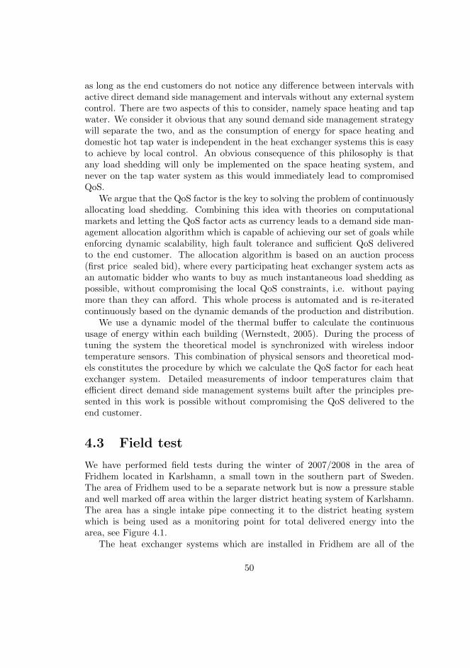
as long as the end customers do not notice any difference between intervals withactive direct demand side management and intervals without any external systemcontrol. There are two aspects of this to consider, namely space heating and tapwater. We consider it obvious that any sound demand side management strategywill separate the two, and as the consumption of energy for space heating anddomestic hot tap water is independent in the heat exchanger systems this is easyto achieve by local control. An obvious consequence of this philosophy is thatany load shedding will only be implemented on the space heating system, andnever on the tap water system as this would immediately lead to compromisedQoS.

We argue that the QoS factor is the key to solving the problem of continuouslyallocating load shedding. Combining this idea with theories on computationalmarkets and letting the QoS factor acts as currency leads to a demand side man-agement allocation algorithm which is capable of achieving our set of goals whileenforcing dynamic scalability, high fault tolerance and sufficient QoS deliveredto the end customer. The allocation algorithm is based on an auction process(first price sealed bid), where every participating heat exchanger system acts asan automatic bidder who wants to buy as much instantaneous load shedding aspossible, without compromising the local QoS constraints, i.e. without payingmore than they can afford. This whole process is automated and is re-iteratedcontinuously based on the dynamic demands of the production and distribution.

We use a dynamic model of the thermal buffer to calculate the continuoususage of energy within each building (Wernstedt, 2005). During the process oftuning the system the theoretical model is synchronized with wireless indoortemperature sensors. This combination of physical sensors and theoretical mod-els constitutes the procedure by which we calculate the QoS factor for each heatexchanger system. Detailed measurements of indoor temperatures claim thatefficient direct demand side management systems built after the principles pre-sented in this work is possible without compromising the QoS delivered to theend customer.

4.3 Field test

We have performed field tests during the winter of 2007/2008 in the area ofFridhem located in Karlshamn, a small town in the southern part of Sweden.The area of Fridhem used to be a separate network but is now a pressure stableand well marked off area within the larger district heating system of Karlshamn.The area has a single intake pipe connecting it to the district heating systemwhich is being used as a monitoring point for total delivered energy into thearea, see Figure 4.1.

The heat exchanger systems which are installed in Fridhem are all of the

50

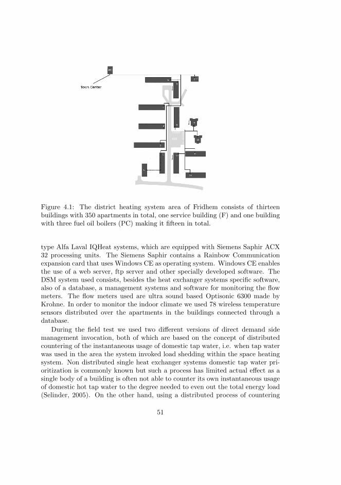
Figure 4.1: The district heating system area of Fridhem consists of thirteenbuildings with 350 apartments in total, one service building (F) and one buildingwith three fuel oil boilers (PC) making it fifteen in total.

type Alfa Laval IQHeat systems, which are equipped with Siemens Saphir ACX32 processing units. The Siemens Saphir contains a Rainbow Communicationexpansion card that uses Windows CE as operating system. Windows CE enablesthe use of a web server, ftp server and other specially developed software. TheDSM system used consists, besides the heat exchanger systems specific software,also of a database, a management systems and software for monitoring the flowmeters. The flow meters used are ultra sound based Optisonic 6300 made byKrohne. In order to monitor the indoor climate we used 78 wireless temperaturesensors distributed over the apartments in the buildings connected through adatabase.

During the field test we used two different versions of direct demand sidemanagement invocation, both of which are based on the concept of distributedcountering of the instantaneous usage of domestic tap water, i.e. when tap waterwas used in the area the system invoked load shedding within the space heatingsystem. Non distributed single heat exchanger systems domestic tap water pri-oritization is commonly known but such a process has limited actual effect as asingle body of a building is often not able to counter its own instantaneous usageof domestic hot tap water to the degree needed to even out the total energy load(Selinder, 2005). On the other hand, using a distributed process of countering

51

such instantaneous usage of domestic hot tap water, several buildings can usetheir combined thermal buffer in order to continuously even out the total en-ergy demand within a district heating system. The two versions of demand sidemanagement invocation are rather similar, i.e. they both trigger on the usageof domestic hot tap water, the main difference being that one of the versionsovercompensated the wanted load level in order to minimize the influence of theusage of domestic hot tap water. The wanted load level is the level that the con-trol system tries to maintain throughout a single day. The level for a specific dayis found by measuring the average load level during a four hour period between02.00 and 06.00 in the night when no demand side management is invoked. Thisperiod is used because the social part of the load is assumed to be low betweenthese hours. During the following day, starting at 06.00, the found average loadlevel is used as a trigger for the control system, i.e. when the load level riseabove the wanted load level the system invokes demand side management. Whenthe system is in continuous use over several days the demand side managementsystem will be active during 06.00 until 02.00 the following night, with non- de-mand side management load level finding periods during the intermediate hours.The wanted load level is different for every day, and since the heat load duringthe night is used mostly for indoor heating the wanted load level will correlateclosely to the outdoor temperature. During overcompensation we lowered thewanted load level by a fixed amount in order to make the system react faster toany demand side management activity, i.e. we forced the system to trigger anauction earlier than otherwise would be the case. Distribution of load sheddingis achieved through the use of the quality filter auction process described in theprevious section. The sequence of work for a single instance of such an auctionis as follows:

I. The input data for decision-making reveals the need for load shedding,which causes the auctioneer entity to prepare an auction process.

II. An auction request, detailing information about the desired load shedding,is distributed among the participating heat exchanger systems.

III. All participating heat exchanger systems respond to the request by bidding,using their QoS factor as currency. Any heat exchanger system can at thispoint opt to refuse to participate in the auction, in which case this is madeclear to the auctioneer.

IV. Based on the bids, the overall system will then choose the winning heat ex-changer system, which is selected to perform the load shedding. More thanone heat exchanger system can be selected in this process, if the situationrequires it, or if they bid similar bids. The resulting information is thendistributed among all participating heat exchanger systems.

52

V. The winning heat exchanger system then implements the current load shed-ding.

This entire process above generally takes less than a second to perform. Theprocess is re-iterated as long as the production strategies at hand require it.

4.4 Results

During the field tests we have evaluated two demand side management strategies,a strategy with and a strategy without overcompensation of the wanted load level.As a reference Figure 4.2 shows the typical heat load during a full day without anyactive demand side management. The peak loads during morning and eveningcan be clearly identified.

Figure 4.2: The typical load without any active demand side management. Thestraight line indicates a wanted load level.

Figure 4.3 shows a demand side management strategy using the actual wantedload level. The expected peak loads during morning and evening are clearlyreduced.

In Figure 4.4 we show the system using an overcompensated wanted load level.Since the wanted load level is overcompensated it will be lower than the actualaverage during the night.

If we compare the two demand side management periods from Figure 4.3and Figure 4.4a notable difference can be seen, in that the period where weovercompensated the wanted load level displays a somewhat more fluctuatingbehaviour. This behaviour arises from the fact that the control process behaves

53

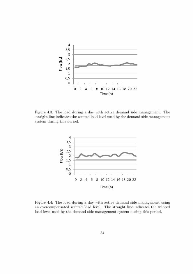
Figure 4.3: The load during a day with active demand side management. Thestraight line indicates the wanted load level used by the demand side managementsystem during this period.

Figure 4.4: The load during a day with active demand side management usingan overcompensated wanted load level. The straight line indicates the wantedload level used by the demand side management system during this period.

54

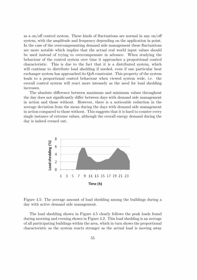
as a on/off control system. These kinds of fluctuations are normal in any on/offsystem, with the amplitude and frequency depending on the application in point.In the case of the overcompensating demand side management these fluctuationsare more notable which implies that the actual real world input values shouldbe used instead of trying to overcompensate in advance. When studying thebehaviour of the control system over time it approaches a proportional controlcharacteristic. This is due to the fact that it is a distributed system, whichwill continue to distribute load shedding if needed, even if one particular heatexchanger system has approached its QoS constraint. This property of the systemleads to a proportional control behaviour when viewed system wide, i.e. theoverall control system will react more intensely as the need for load sheddingincreases.

The absolute difference between maximum and minimum values throughoutthe day does not significantly differ between days with demand side managementin action and those without. However, there is a noticeable reduction in theaverage deviation from the mean during the days with demand side managementin action compared to those without. This suggests that it is hard to counter everysingle instance of extreme values, although the overall energy demand during theday is indeed evened out.

Figure 4.5: The average amount of load shedding among the buildings during aday with active demand side management.

The load shedding shown in Figure 4.5 clearly follows the peak loads foundduring morning and evening shown in Figure 4.2. This load shedding is an averageof all participating buildings within the area, which in turn shows the proportionalcharacteristic as the system reacts stronger as the actual load is moving away

55

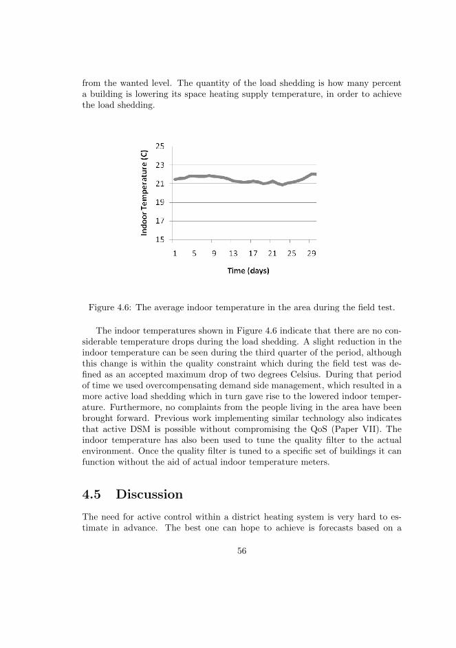
from the wanted level. The quantity of the load shedding is how many percenta building is lowering its space heating supply temperature, in order to achievethe load shedding.

Figure 4.6: The average indoor temperature in the area during the field test.

The indoor temperatures shown in Figure 4.6 indicate that there are no con-siderable temperature drops during the load shedding. A slight reduction in theindoor temperature can be seen during the third quarter of the period, althoughthis change is within the quality constraint which during the field test was de-fined as an accepted maximum drop of two degrees Celsius. During that periodof time we used overcompensating demand side management, which resulted in amore active load shedding which in turn gave rise to the lowered indoor temper-ature. Furthermore, no complaints from the people living in the area have beenbrought forward. Previous work implementing similar technology also indicatesthat active DSM is possible without compromising the QoS (Paper VII). Theindoor temperature has also been used to tune the quality filter to the actualenvironment. Once the quality filter is tuned to a specific set of buildings it canfunction without the aid of actual indoor temperature meters.

4.5 Discussion

The need for active control within a district heating system is very hard to es-timate in advance. The best one can hope to achieve is forecasts based on a

56

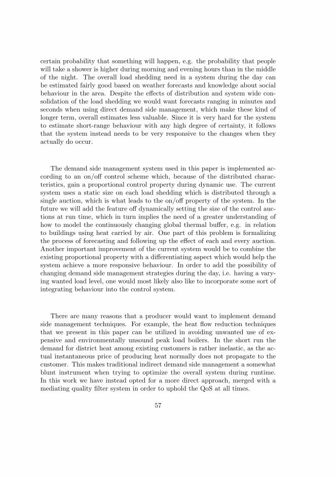
certain probability that something will happen, e.g. the probability that peoplewill take a shower is higher during morning and evening hours than in the middleof the night. The overall load shedding need in a system during the day canbe estimated fairly good based on weather forecasts and knowledge about socialbehaviour in the area. Despite the effects of distribution and system wide con-solidation of the load shedding we would want forecasts ranging in minutes andseconds when using direct demand side management, which make these kind oflonger term, overall estimates less valuable. Since it is very hard for the systemto estimate short-range behaviour with any high degree of certainty, it followsthat the system instead needs to be very responsive to the changes when theyactually do occur.

The demand side management system used in this paper is implemented ac-cording to an on/off control scheme which, because of the distributed charac-teristics, gain a proportional control property during dynamic use. The currentsystem uses a static size on each load shedding which is distributed through asingle auction, which is what leads to the on/off property of the system. In thefuture we will add the feature off dynamically setting the size of the control auc-tions at run time, which in turn implies the need of a greater understanding ofhow to model the continuously changing global thermal buffer, e.g. in relationto buildings using heat carried by air. One part of this problem is formalizingthe process of forecasting and following up the effect of each and every auction.Another important improvement of the current system would be to combine theexisting proportional property with a differentiating aspect which would help thesystem achieve a more responsive behaviour. In order to add the possibility ofchanging demand side management strategies during the day, i.e. having a vary-ing wanted load level, one would most likely also like to incorporate some sort ofintegrating behaviour into the control system.

There are many reasons that a producer would want to implement demandside management techniques. For example, the heat flow reduction techniquesthat we present in this paper can be utilized in avoiding unwanted use of ex-pensive and environmentally unsound peak load boilers. In the short run thedemand for district heat among existing customers is rather inelastic, as the ac-tual instantaneous price of producing heat normally does not propagate to thecustomer. This makes traditional indirect demand side management a somewhatblunt instrument when trying to optimize the overall system during runtime.In this work we have instead opted for a more direct approach, merged with amediating quality filter system in order to uphold the QoS at all times.

57

4.6 Conclusions

In this paper we have introduced a framework for merging direct demand sidemanagement with considerations to QoS, and shown the value of cooperationamong heat exchanger systems in a district heating system. We have presenteda demand side management system which is able to even out fluctuations in thedaily energy load. Detailed measurements of indoor temperatures claim thatefficient demand side management based on the principles presented in this workis possible without compromising the QoS delivered to the customer.

During the field test we have had a production oriented strategy in focus, i.e.to achieve an even heat load during the day within the entire area. The goal wasnot explicitly to minimize the heating cost in every specific participating heatexchanger system, even if a lowering effect on the heat usage in each buildingobviously will occur when one lowers the overall heat load. In previous work wehave studied more consumer oriented demand side management strategies (PaperII), and we have shown that similar demand side management techniques can beused in order to optimize the heat usage from a customer perspective where theoverall goal is to minimize the actual heating cost, again without compromisingthe QoS. From a purely technical viewpoint, there is no conflict in using differentstrategies like these at the same time, as the mediating quality filter will activateto insure that the QoS is not being compromised in either way.

Monitoring systems for district heating system are already very complex andcomprehensive systems which we believe are going to become even more sophis-ticated in the future. This is due to the possibilities in increasing computationaland communication performance in combination with more refined sensory equip-ment producing more elaborate data. Correctly designed and implemented thisevolving trend can and, most likely, will contribute considerable to the optimalperformance of the district heating system and any demand side managementstrategies. Using a fully distributed control and monitoring system like this wouldgive individual consumers real-time information about their energy demand andcontinuous energy pricing, and would create the possibility of complete trans-parency in the pricing model which could benefit both producer and customer.

The results presented in this paper promise both economical and environmen-tal benefits as well as a win-win situation for the district heating provider andthe customers. All possibilities have to be considered when trying to increasethe market share of district heating system and quality ensured demand sidemanagement should be regarded as part of any competitive and efficient districtheating system.

58

Chapter 5

Paper IV - A case study onavailability of sensor data inagent cooperation

Multi-agent cooperation can in several cases be used in order to mitigate prob-lems relating to task sharing within physical processes. In this paper we applyagent based solutions to a class of problems defined by their property of being pre-dictable from a macroscopic perspective while being highly stochastic when viewedat a microscopic level. These characteristic properties can be found in severalindustrial processes and applications, e.g. within the energy market where theproduction and distribution of electricity follow this pattern. Another definingproblem characteristic is that the supply is usually limited as well as consisting ofseveral layers of differentiating production costs. We evaluate and compare theperformance of the agent system in three different scenarios, and for each suchscenario it is shown to what degree the optimization system is dependent on thelevel of availability of sensor data

5.1 Keyworks

Agent co-operation, Team work

59

5.2 Introduction

Schemes for sustaining cooperative behavior among agents are often dependenton a certain level of communication in order to establish and maintain a recip-rocal sense of trust. However, in real-life applications it is not always possible touphold the desired level of availability and quality of data being communicatedamong the agents, thus causing suboptimal cooperative behavior. In this paperwe focus on a problem domain where multi-agent task sharing cooperative behav-ior is applied. However, as practical implementations within this domain oftenare spread geographically over a wide area and lack dedicated network communi-cation infrastructure, there are often practical limitations on the availability andquality of sensor data which in turn limits the effectiveness of the multi-agentsystem cooperative behavior.

For agents to effectively coordinate their actions, the agents normally needto share information. Information sharing, i.e. communication and its effecton overall performance is a well established area and has been studied by sev-eral researchers (Dutta, Goldman, & Jennings, 2007), (Goldman & Zilberstein,2003) and (Shen, Lesser, & Carver, 2003). Also,the area of multi-sensor net-works and sensor data quality and fusion has received a fair amount of interest(Dash, Rogers, S., Roberts, & Jennings, 2005), (Lesser, Ortiz, & Tambe, 2003)and (Jayasima, 1996). However, the quality of information in combination withinformation sharing has so far, to our knowledge, only received little attention.

5.2.1 Problem domain

The problem domain is characterised by being predictable from a macroscopicperspective while being stochastic when viewed at a microscopic level. As themacroscopic behaviour is a reflection of a collection of highly stochastic micro-scopic events which in themselves cannot be predicted, it follows that althougha process control system is able to foresee general trends and tendencies withinthe process, it must be able to handle the stochastic behaviour in order to actu-ally manipulate the process. For example, although it is possible to foresee theoverall heating demand within a building being higher tomorrow as the weatherprognosis shows a drop in outdoor temperature, it is not possible to predict whenindividual residents will take a shower, thus creating peak loads in the total en-ergy demand when combining usage of hot tap water and space heating. Basicallythese processes are driven by one or more producers supplying some kind of utilityand one or more consumers acting to satisfy their own demand of the utility.

When optimizing the operational production one tries to determine the finan-cially and operationally most efficient way to combine the production resources,while satisfying the consumer needs. This problem is often formalized by us-ing the Economic Dispatch Problem (EDP) and the Unit Commitment Problem

60

(UCP) (Dotzauer, 2002). By solving the EDP we find out how much load to gen-erate by each of the different available production units at a given time. Sincemost production units in real life settings cannot be turned on and off at theblink of an eye, it is important to plan ahead of time and determine which unitsneed to be started, when they need to be started and how long they should becommitted to being in use, i.e. solving the UCP. These problems are related toeach other and are solved using similar optimization techniques. A complicatingfactor when optimizing production is that the production costs usually displaynon-linear patterns, due to physical processes like valve effects and the usage ofdifferently priced fuels in production. This leads to objective functions with dis-continuous and non-differentiable points, which means that it is generally moreappropriate to treat the cost function as a set of piecewise quadratic functions(Koay et al., 2008), (C.E. & G.L., 1984). As demand rises the producing entityis forced to engage increasingly costly production units, and eventually the pro-duction costs exceed the possible sale price of the utility. The only way for theproducer to mitigate such a situation is to manipulate consumption in order tolower the demand.

By solving the UCP and EDP the producer finds an optimal production strat-egy for a given time frame, e.g. the next twenty-four hours. This means thatthe producer wants the consumption to be as close to this strategy as possible;if the consumption falls to low it will result in unnecessarily low income, while atoo high consumption will necessitate starting costly peak load production units.In order to achieve and uphold the desired production strategy multi agent sys-tems and other distributed systems can be used to manage the consumption.We evaluate the success of such systems by measuring their ability to stick tothe production strategy in question, while at the same time satisfying consumerdemand.

Typically the consumer entity has a wanted state which it tries to upholdat all times. This wanted state is dependent on the physical environment inwhich the system is functioning, e.g. maintaining comfortable indoor climate ina district heating system. Often, however, a consumer agent can accept smallerdeviations from this wanted state during shorter periods of time. This is whatmakes it possible for a control system to manage the society of consumers inorder to achieve some local or global goals. By measuring the deviation from thewanted state it is possible to evaluate the impact of change in the overall systemcaused by individual consumers.

5.2.2 Problem description

The consumption, and thus the production, follows certain patterns which arepredictable to some extent from a system wide perspective. These patterns are

61

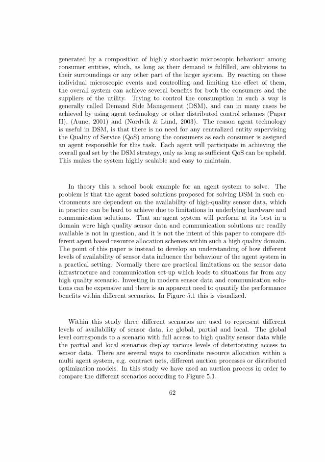
generated by a composition of highly stochastic microscopic behaviour amongconsumer entities, which, as long as their demand is fulfilled, are oblivious totheir surroundings or any other part of the larger system. By reacting on theseindividual microscopic events and controlling and limiting the effect of them,the overall system can achieve several benefits for both the consumers and thesuppliers of the utility. Trying to control the consumption in such a way isgenerally called Demand Side Management (DSM), and can in many cases beachieved by using agent technology or other distributed control schemes (PaperII), (Aune, 2001) and (Nordvik & Lund, 2003). The reason agent technologyis useful in DSM, is that there is no need for any centralized entity supervisingthe Quality of Service (QoS) among the consumers as each consumer is assignedan agent responsible for this task. Each agent will participate in achieving theoverall goal set by the DSM strategy, only as long as sufficient QoS can be upheld.This makes the system highly scalable and easy to maintain.

In theory this a school book example for an agent system to solve. Theproblem is that the agent based solutions proposed for solving DSM in such en-vironments are dependent on the availability of high-quality sensor data, whichin practice can be hard to achieve due to limitations in underlying hardware andcommunication solutions. That an agent system will perform at its best in adomain were high quality sensor data and communication solutions are readilyavailable is not in question, and it is not the intent of this paper to compare dif-ferent agent based resource allocation schemes within such a high quality domain.The point of this paper is instead to develop an understanding of how differentlevels of availability of sensor data influence the behaviour of the agent system ina practical setting. Normally there are practical limitations on the sensor datainfrastructure and communication set-up which leads to situations far from anyhigh quality scenario. Investing in modern sensor data and communication solu-tions can be expensive and there is an apparent need to quantify the performancebenefits within different scenarios. In Figure 5.1 this is visualized.

Within this study three different scenarios are used to represent differentlevels of availability of sensor data, i.e global, partial and local. The globallevel corresponds to a scenario with full access to high quality sensor data whilethe partial and local scenarios display various levels of deteriorating access tosensor data. There are several ways to coordinate resource allocation within amulti agent system, e.g. contract nets, different auction processes or distributedoptimization models. In this study we have used an auction process in order tocompare the different scenarios according to Figure 5.1.

62

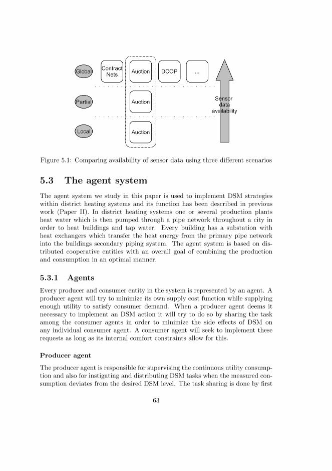
Figure 5.1: Comparing availability of sensor data using three different scenarios

5.3 The agent system

The agent system we study in this paper is used to implement DSM strategieswithin district heating systems and its function has been described in previouswork (Paper II). In district heating systems one or several production plantsheat water which is then pumped through a pipe network throughout a city inorder to heat buildings and tap water. Every building has a substation withheat exchangers which transfer the heat energy from the primary pipe networkinto the buildings secondary piping system. The agent system is based on dis-tributed cooperative entities with an overall goal of combining the productionand consumption in an optimal manner.

5.3.1 Agents

Every producer and consumer entity in the system is represented by an agent. Aproducer agent will try to minimize its own supply cost function while supplyingenough utility to satisfy consumer demand. When a producer agent deems itnecessary to implement an DSM action it will try to do so by sharing the taskamong the consumer agents in order to minimize the side effects of DSM onany individual consumer agent. A consumer agent will seek to implement theserequests as long as its internal comfort constraints allow for this.

Producer agent

The producer agent is responsible for supervising the continuous utility consump-tion and also for instigating and distributing DSM tasks when the measured con-sumption deviates from the desired DSM level. The task sharing is done by first

63

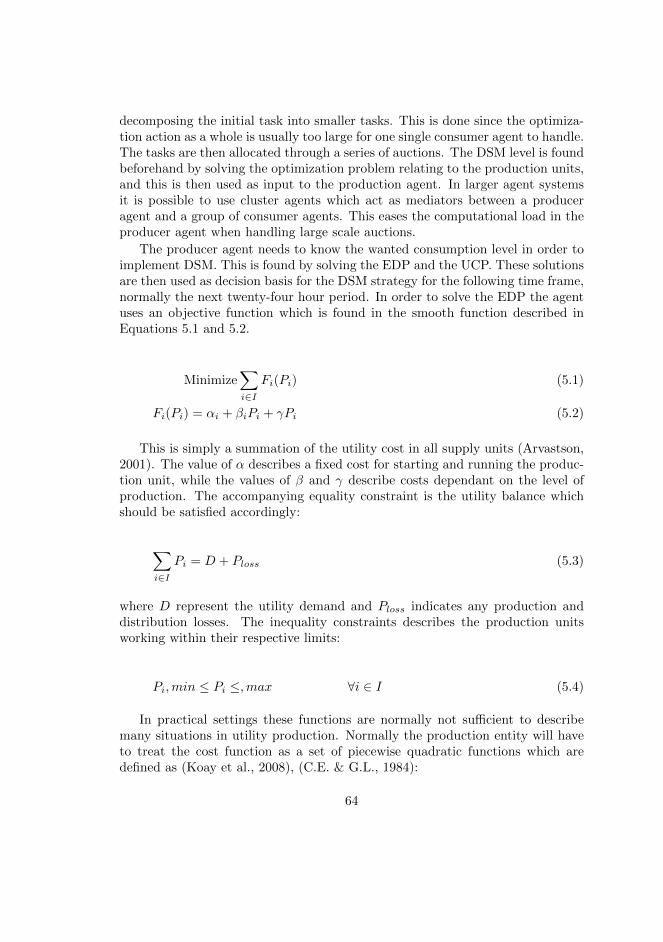
decomposing the initial task into smaller tasks. This is done since the optimiza-tion action as a whole is usually too large for one single consumer agent to handle.The tasks are then allocated through a series of auctions. The DSM level is foundbeforehand by solving the optimization problem relating to the production units,and this is then used as input to the production agent. In larger agent systemsit is possible to use cluster agents which act as mediators between a produceragent and a group of consumer agents. This eases the computational load in theproducer agent when handling large scale auctions.

The producer agent needs to know the wanted consumption level in order toimplement DSM. This is found by solving the EDP and the UCP. These solutionsare then used as decision basis for the DSM strategy for the following time frame,normally the next twenty-four hour period. In order to solve the EDP the agentuses an objective function which is found in the smooth function described inEquations 5.1 and 5.2.

Minimize∑i∈I

Fi(Pi) (5.1)

Fi(Pi) = αi + βiPi + γPi (5.2)

This is simply a summation of the utility cost in all supply units (Arvastson,2001). The value of α describes a fixed cost for starting and running the produc-tion unit, while the values of β and γ describe costs dependant on the level ofproduction. The accompanying equality constraint is the utility balance whichshould be satisfied accordingly:

∑i∈I

Pi = D + Ploss (5.3)

where D represent the utility demand and Ploss indicates any production anddistribution losses. The inequality constraints describes the production unitsworking within their respective limits:

Pi,min ≤ Pi ≤,max ∀i ∈ I (5.4)

In practical settings these functions are normally not sufficient to describemany situations in utility production. Normally the production entity will haveto treat the cost function as a set of piecewise quadratic functions which aredefined as (Koay et al., 2008), (C.E. & G.L., 1984):

64

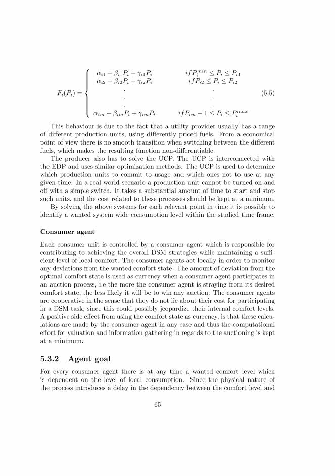
Fi(Pi) =

αi1 + βi1Pi + γi1Pi ifPmini ≤ Pi ≤ Pi1αi2 + βi2Pi + γi2Pi ifPi2 ≤ Pi ≤ Pi2

. .

. .

. .αim + βimPi + γimPi ifPim − 1 ≤ Pi ≤ Pmaxi

(5.5)

This behaviour is due to the fact that a utility provider usually has a rangeof different production units, using differently priced fuels. From a economicalpoint of view there is no smooth transition when switching between the differentfuels, which makes the resulting function non-differentiable.

The producer also has to solve the UCP. The UCP is interconnected withthe EDP and uses similar optimization methods. The UCP is used to determinewhich production units to commit to usage and which ones not to use at anygiven time. In a real world scenario a production unit cannot be turned on andoff with a simple switch. It takes a substantial amount of time to start and stopsuch units, and the cost related to these processes should be kept at a minimum.

By solving the above systems for each relevant point in time it is possible toidentify a wanted system wide consumption level within the studied time frame.

Consumer agent

Each consumer unit is controlled by a consumer agent which is responsible forcontributing to achieving the overall DSM strategies while maintaining a suffi-cient level of local comfort. The consumer agents act locally in order to monitorany deviations from the wanted comfort state. The amount of deviation from theoptimal comfort state is used as currency when a consumer agent participates inan auction process, i.e the more the consumer agent is straying from its desiredcomfort state, the less likely it will be to win any auction. The consumer agentsare cooperative in the sense that they do not lie about their cost for participatingin a DSM task, since this could possibly jeopardize their internal comfort levels.A positive side effect from using the comfort state as currency, is that these calcu-lations are made by the consumer agent in any case and thus the computationaleffort for valuation and information gathering in regards to the auctioning is keptat a minimum.

5.3.2 Agent goal

For every consumer agent there is at any time a wanted comfort level whichis dependent on the level of local consumption. Since the physical nature ofthe process introduces a delay in the dependency between the comfort level and

65

the local consumption level a time frame is created within which it is possibleto manipulate the local consumption while still keeping the local comfort levelwithin its constraints. An example of this phenomena is that it will take sometime before people notice if you shut off the radiators in a building, i.e. thereis a delay before the people start to freeze even though the energy consumptionis reduced directly. Combining the local consumption from each consumer agentwill yield the total actual consumption. The goal for the agent system is then; foreach point in time to achieve a total actual consumption as close as possible tothe total wanted consumption while keeping all local comfort levels within theirindividual constraints.

In a steady state system this could be seen as a traditional optimizationproblem, i.e. to find a optimum between two conflicting objective functions.However, since we are dealing with a dynamic system the aspects of adaptationand re-planning becomes important, which requires a more sophisticated solution.

5.3.3 Auction process

Whenever a producer agent needs to implement a DSM action it will distributethis by using a private value first priced, sealed bid auction process. For theconsumer agent the value is to implement as much DSM tasks as possible, and thecurrency used is the amount of deviation from the optimal comfort state possiblewithout affecting the local QoS. This type of auction based multi agent systemhas previously been successfully implemented in district heating networks in orderto achieve DSM (Paper III). Strategic decisions are made based on global orlocal views within the environment, and the specific optimization actions rely oncontinuous sensor data. Global knowledge is needed in order to identify individualconsumer agents able and willing to participate in local task accomplishment.Without sufficient communication abilities the auction process is not able tofunction, thus making it more difficult to distribute DSM tasks while taking intoaccount the local consumer agent comfort state. By using an action process it ispossible to distribute the complexity and computational effort, since all reasoningand planning about the delivered QoS is done by the consumer agents. This leadsto a more scalable and extendable system.

5.3.4 Levels of agent knowledge

In the described DSM system the agents are able to communicate freely amongtheir peers, in order to continuously propagate system status based on availablesensor data and perform coordinated task sharing when needed. In this studywe compare the performance of such a fully functional system with two othersystems displaying increasingly worse availability of sensor data. These threedifferent scenarios are based on the level of system wide knowledge available to

66

the participating agents; global, partial and local. We choose to compare thesespecific three levels of system wide knowledge because they correspond to infras-tructural prerequisites which can normally be found in actual physical systems,and because they display a broad and clear view of the problem discussed.

Global knowledge

This is the normal operational view for the MAS used to operate the DSM strate-gies. The producer agents are able to continuously supervise the use of productionutility and are able to instigate DSM actions as need arises. Each DSM actionis divided into control tasks which can be distributed throughout the networkof consumer agents by system wide auctions. The consumer agents are able touphold their individual QoS by deciding when and how to participate in theseauctions, i.e. a DSM task is never forced upon a consumer agent against its will.

Partial knowledge

The producer agents are able to supervise the consumption of production utility,but they are not able to communicate local sensory data with consumer agents.This means that cooperative behaviour through auctioning is not possible. Aproducer agent is, however, still able to instigate uninformed DSM actions. Thisis normally done by using predefined activation lists, which force consumer agentsto implement DSM tasks in a round-robin fashion. Since no communication ofconsumer sensor data is available it is not possible for the producer agents togain any feedback about the impact of these DSM tasks on the QoS delivered tothe local consumer. The local consumer agent is still working to uphold its ownQoS, and it might decide not to implement the DSM task appointed to it. Eitherway, as the consumer sensor data communication is impaired, the producer agentwill never gain any knowledge about what decision the consumer agent takes.

Local knowledge

In this scenario the producer agents have little or no knowledge about the contin-uous consumption of production utility, and they do not have any possibility atall to implement any DSM actions, either by cooperation or force. The consumeragents still have access to their own local sensor data but they cannot success-fully communicate this to other agents within the MAS. This basically meansthat they act oblivious to the state of any other agent. In such a system theconsumer agents are often assigned the task of keeping the local utility use toa minimum while upholding the desired QoS. Depending on the situation suchbehaviour might or might not be for the good of the global system state, but theconsumer agent will never know anything about this.

67

5.4 The experiment

In this study we investigate the effects of different levels of availability of sensordata within an operational agent based control system. Under normal circum-stances the agent system is based on cooperative behaviour which is in turn heav-ily dependent on functioning and reliable communication of high quality sensordata. Performance of the multi-agent system will deteriorate if the availability orquality of sensor data declines. We have studied how extensive this deteriorationwill be in a practical setting, i.e. how will the quality of the communication un-derlying the decision-making affect the overall performance from a system wideperspective. The case study is based on operational data from an agent basedcontrol system operational in a district heating network in the town of Karlshamnin the south of Sweden (Paper II), (Paper III). This data is used as input whensimulating the various scenarios described in the previous sections.

5.4.1 Reference data

District heating networks are good examples of the described problem domainas they display most, if not all, of the mentioned characteristics. The referencedata in question is collected during a twenty-four hour period with no DSMstrategy active, i.e. no external control is applied to the consumers. The datais representative of normal usage during wintertime when the heating demand issubstantial. The energy consumption in a district heating system is measuredby combining the flow of the water with the primary supply temperature of thewater. During the course of a single day the primary supply temperature in thisdistrict heating network is rather constant so the flow is a good estimate of thetotal energy use.

Figure 5.2 shows the flow data from the Karlshamn district heating networkduring a full twenty-four hour time period. The straight dashed line shows thecalculated wanted level of energy consumption which the producer agent uses asa benchmark during this specific day. This level of consumption is based on asolution of the Economic Dispatch Problem and the Unit Commitment Problem.The peaks above the dashed line represents peak loads which would need to besatisfied by using financially and environmentally unsound fossil fuel. In otherwords, the global goal of the agent system is to keep the consumption as close tothe straight dashed line as possible.

5.4.2 Utility evalution

The consumer agents all have different comfort constraints based on a functionof size, shape and material of the individual building, i.e. the amount of thermalbuffer available (Olsson Ingvarsson & Werner, 2008). In the operational system

68

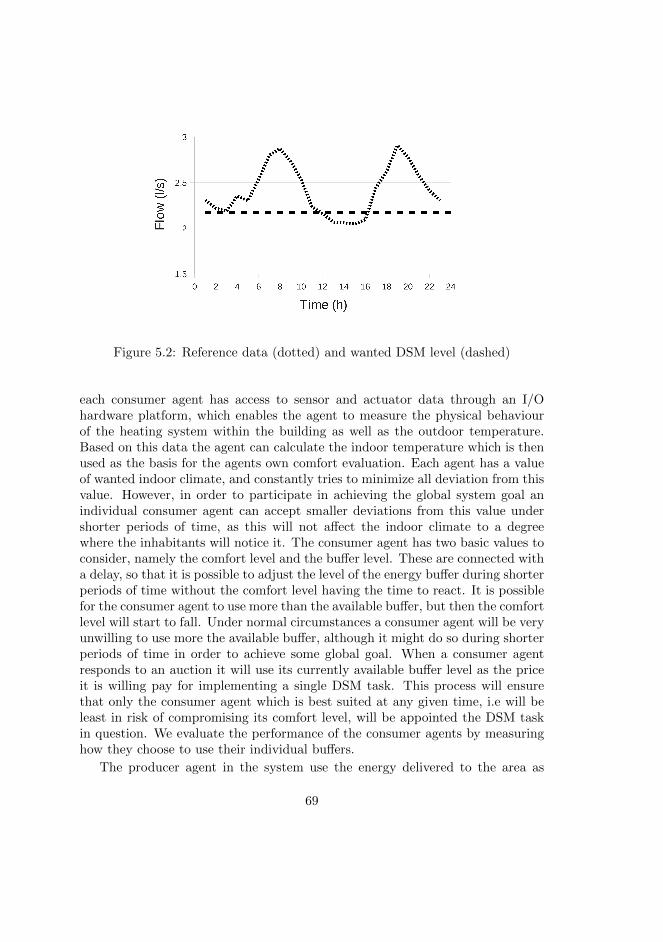
Figure 5.2: Reference data (dotted) and wanted DSM level (dashed)

each consumer agent has access to sensor and actuator data through an I/Ohardware platform, which enables the agent to measure the physical behaviourof the heating system within the building as well as the outdoor temperature.Based on this data the agent can calculate the indoor temperature which is thenused as the basis for the agents own comfort evaluation. Each agent has a valueof wanted indoor climate, and constantly tries to minimize all deviation from thisvalue. However, in order to participate in achieving the global system goal anindividual consumer agent can accept smaller deviations from this value undershorter periods of time, as this will not affect the indoor climate to a degreewhere the inhabitants will notice it. The consumer agent has two basic values toconsider, namely the comfort level and the buffer level. These are connected witha delay, so that it is possible to adjust the level of the energy buffer during shorterperiods of time without the comfort level having the time to react. It is possiblefor the consumer agent to use more than the available buffer, but then the comfortlevel will start to fall. Under normal circumstances a consumer agent will be veryunwilling to use more the available buffer, although it might do so during shorterperiods of time in order to achieve some global goal. When a consumer agentresponds to an auction it will use its currently available buffer level as the priceit is willing pay for implementing a single DSM task. This process will ensurethat only the consumer agent which is best suited at any given time, i.e will beleast in risk of compromising its comfort level, will be appointed the DSM taskin question. We evaluate the performance of the consumer agents by measuringhow they choose to use their individual buffers.

The producer agent in the system use the energy delivered to the area as

69

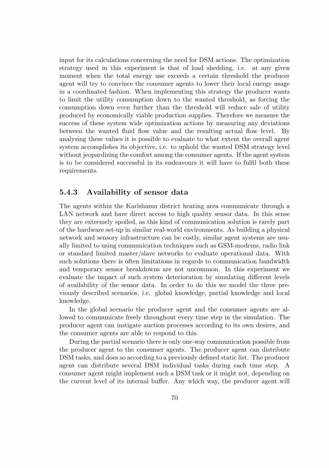
input for its calculations concerning the need for DSM actions. The optimizationstrategy used in this experiment is that of load shedding, i.e. at any givenmoment when the total energy use exceeds a certain threshold the produceragent will try to convince the consumer agents to lower their local energy usagein a coordinated fashion. When implementing this strategy the producer wantsto limit the utility consumption down to the wanted threshold, as forcing theconsumption down even further than the threshold will reduce sale of utilityproduced by economically viable production supplies. Therefore we measure thesuccess of these system wide optimization actions by measuring any deviationsbetween the wanted fluid flow value and the resulting actual flow level. Byanalysing these values it is possible to evaluate to what extent the overall agentsystem accomplishes its objective, i.e. to uphold the wanted DSM strategy levelwithout jeopardizing the comfort among the consumer agents. If the agent systemis to be considered successful in its endeavours it will have to fulfil both theserequirements.

5.4.3 Availability of sensor data

The agents within the Karlshamn district heating area communicate through aLAN network and have direct access to high quality sensor data. In this sensethey are extremely spoiled, as this kind of communication solution is rarely partof the hardware set-up in similar real-world environments. As building a physicalnetwork and sensory infrastructure can be costly, similar agent systems are usu-ally limited to using communication techniques such as GSM-modems, radio linkor standard limited master/slave networks to evaluate operational data. Withsuch solutions there is often limitations in regards to communication bandwidthand temporary sensor breakdowns are not uncommon. In this experiment weevaluate the impact of such system deterioration by simulating different levelsof availability of the sensor data. In order to do this we model the three pre-viously described scenarios, i.e. global knowledge, partial knowledge and localknowledge.

In the global scenario the producer agent and the consumer agents are al-lowed to communicate freely throughout every time step in the simulation. Theproducer agent can instigate auction processes according to its own desires, andthe consumer agents are able to respond to this.

During the partial scenario there is only one-way communication possible fromthe producer agent to the consumer agents. The producer agent can distributeDSM tasks, and does so according to a previously defined static list. The produceragent can distribute several DSM individual tasks during each time step. Aconsumer agent might implement such a DSM task or it might not, depending onthe current level of its internal buffer. Any which way, the producer agent will

70

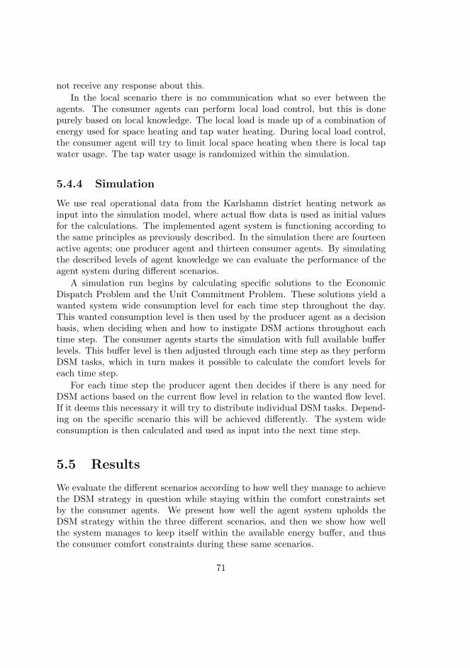
not receive any response about this.

In the local scenario there is no communication what so ever between theagents. The consumer agents can perform local load control, but this is donepurely based on local knowledge. The local load is made up of a combination ofenergy used for space heating and tap water heating. During local load control,the consumer agent will try to limit local space heating when there is local tapwater usage. The tap water usage is randomized within the simulation.

5.4.4 Simulation

We use real operational data from the Karlshamn district heating network asinput into the simulation model, where actual flow data is used as initial valuesfor the calculations. The implemented agent system is functioning according tothe same principles as previously described. In the simulation there are fourteenactive agents; one producer agent and thirteen consumer agents. By simulatingthe described levels of agent knowledge we can evaluate the performance of theagent system during different scenarios.

A simulation run begins by calculating specific solutions to the EconomicDispatch Problem and the Unit Commitment Problem. These solutions yield awanted system wide consumption level for each time step throughout the day.This wanted consumption level is then used by the producer agent as a decisionbasis, when deciding when and how to instigate DSM actions throughout eachtime step. The consumer agents starts the simulation with full available bufferlevels. This buffer level is then adjusted through each time step as they performDSM tasks, which in turn makes it possible to calculate the comfort levels foreach time step.

For each time step the producer agent then decides if there is any need forDSM actions based on the current flow level in relation to the wanted flow level.If it deems this necessary it will try to distribute individual DSM tasks. Depend-ing on the specific scenario this will be achieved differently. The system wideconsumption is then calculated and used as input into the next time step.

5.5 Results

We evaluate the different scenarios according to how well they manage to achievethe DSM strategy in question while staying within the comfort constraints setby the consumer agents. We present how well the agent system upholds theDSM strategy within the three different scenarios, and then we show how wellthe system manages to keep itself within the available energy buffer, and thusthe consumer comfort constraints during these same scenarios.

71

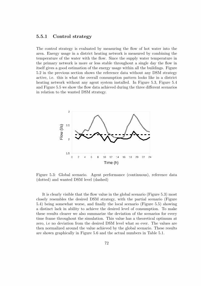
5.5.1 Control strategy

The control strategy is evaluated by measuring the flow of hot water into thearea. Energy usage in a district heating network is measured by combining thetemperature of the water with the flow. Since the supply water temperature inthe primary network is more or less stable throughout a single day the flow initself gives a good estimation of the energy usage within all the buildings. Figure5.2 in the previous section shows the reference data without any DSM strategyactive, i.e. this is what the overall consumption pattern looks like in a districtheating network without any agent system installed. In Figure 5.3, Figure 5.4and Figure 5.5 we show the flow data achieved during the three different scenariosin relation to the wanted DSM strategy.

Figure 5.3: Global scenario. Agent performance (continuous), reference data(dotted) and wanted DSM level (dashed)

It is clearly visible that the flow value in the global scenario (Figure 5.3) mostclosely resembles the desired DSM strategy, with the partial scenario (Figure5.4) being somewhat worse, and finally the local scenario (Figure 5.5) showinga distinct lack in ability to achieve the desired level of consumption. To makethese results clearer we also summarize the deviation of the scenarios for everytime frame throughout the simulation. This value has a theoretical optimum atzero, i.e no deviation from the desired DSM level what so ever. The values arethen normalized around the value achieved by the global scenario. These resultsare shown graphically in Figure 5.6 and the actual numbers in Table 5.1.

72

Figure 5.4: Partial scenario. Agent performance (continuous), reference data(dotted) and wanted DSM level (dashed)

Figure 5.5: Local scenario. Agent performance (continuous), reference data (dot-ted) and wanted DSM level (dashed)

5.5.2 Agent buffer usage

The level of comfort is dependent on the buffer used by each individual consumeragent. Every agent has an maximum allowed buffer usage of 1, with a minimumof 0. The level of comfort will not be negatively effected by a usage between 1

73

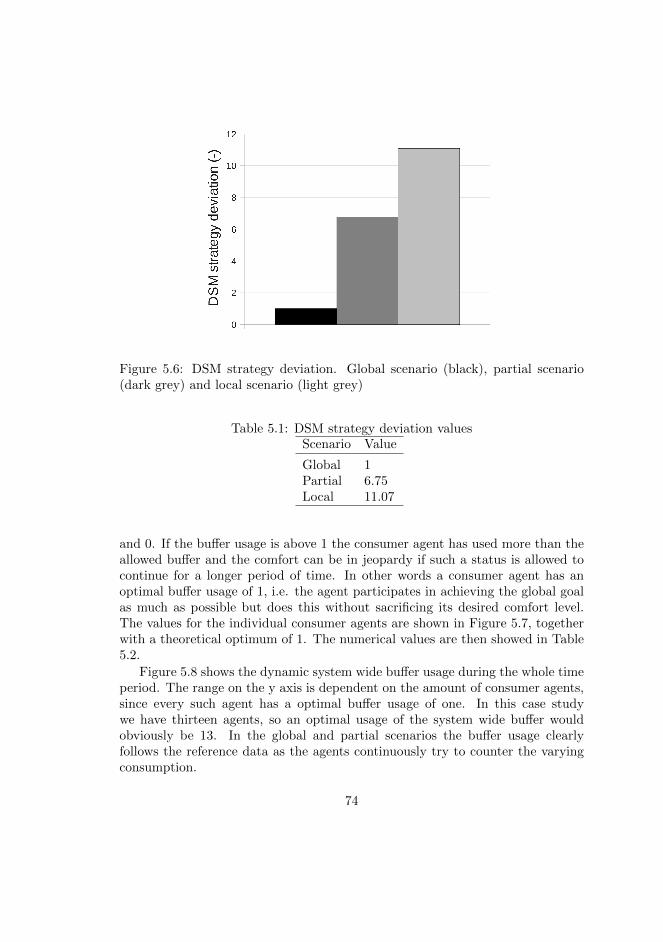
Figure 5.6: DSM strategy deviation. Global scenario (black), partial scenario(dark grey) and local scenario (light grey)

Table 5.1: DSM strategy deviation valuesScenario Value

Global 1Partial 6.75Local 11.07

and 0. If the buffer usage is above 1 the consumer agent has used more than theallowed buffer and the comfort can be in jeopardy if such a status is allowed tocontinue for a longer period of time. In other words a consumer agent has anoptimal buffer usage of 1, i.e. the agent participates in achieving the global goalas much as possible but does this without sacrificing its desired comfort level.The values for the individual consumer agents are shown in Figure 5.7, togetherwith a theoretical optimum of 1. The numerical values are then showed in Table5.2.

Figure 5.8 shows the dynamic system wide buffer usage during the whole timeperiod. The range on the y axis is dependent on the amount of consumer agents,since every such agent has a optimal buffer usage of one. In this case studywe have thirteen agents, so an optimal usage of the system wide buffer wouldobviously be 13. In the global and partial scenarios the buffer usage clearlyfollows the reference data as the agents continuously try to counter the varyingconsumption.

74

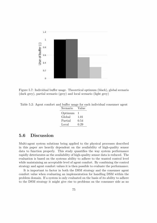
Figure 5.7: Individual buffer usage. Theoretical optimum (black), global scenario(dark grey), partial scenario (grey) and local scenario (light grey)

Table 5.2: Agent comfort and buffer usage for each individual consumer agentScenario Value

Optimum 1Global 1.01Partial 0.54Local 0.29

5.6 Discussion

Multi-agent system solutions being applied to the physical processes describedin this paper are heavily dependent on the availability of high-quality sensordata to function properly. This study quantifies the way system performancerapidly deteriorates as the availability of high-quality sensor data is reduced. Theevaluation is based on the systems ability to adhere to the wanted control levelwhile maintaining an acceptable level of agent comfort. By combining the controlstrategy and agent comfort values it is then possible to evaluate the performance.

It is important to factor in both the DSM strategy and the consumer agentcomfort value when evaluating an implementation for handling DSM within theproblem domain. If a system is only evaluated on the basis of its ability to adhereto the DSM strategy it might give rise to problems on the consumer side as no

75

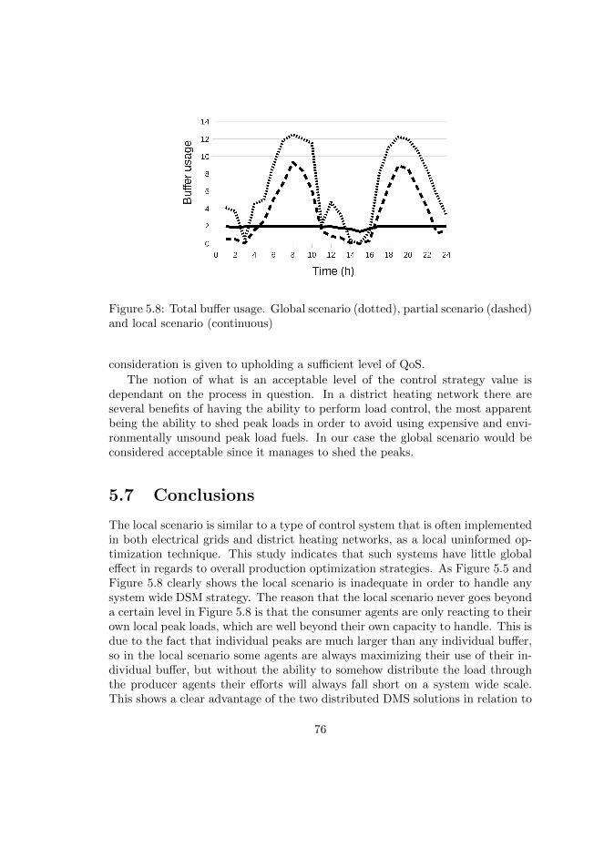
Figure 5.8: Total buffer usage. Global scenario (dotted), partial scenario (dashed)and local scenario (continuous)

consideration is given to upholding a sufficient level of QoS.

The notion of what is an acceptable level of the control strategy value isdependant on the process in question. In a district heating network there areseveral benefits of having the ability to perform load control, the most apparentbeing the ability to shed peak loads in order to avoid using expensive and envi-ronmentally unsound peak load fuels. In our case the global scenario would beconsidered acceptable since it manages to shed the peaks.

5.7 Conclusions

The local scenario is similar to a type of control system that is often implementedin both electrical grids and district heating networks, as a local uninformed op-timization technique. This study indicates that such systems have little globaleffect in regards to overall production optimization strategies. As Figure 5.5 andFigure 5.8 clearly shows the local scenario is inadequate in order to handle anysystem wide DSM strategy. The reason that the local scenario never goes beyonda certain level in Figure 5.8 is that the consumer agents are only reacting to theirown local peak loads, which are well beyond their own capacity to handle. This isdue to the fact that individual peaks are much larger than any individual buffer,so in the local scenario some agents are always maximizing their use of their in-dividual buffer, but without the ability to somehow distribute the load throughthe producer agents their efforts will always fall short on a system wide scale.This shows a clear advantage of the two distributed DMS solutions in relation to

76

any local efforts, which can never hope to counter system wide peaks.

Figure 5.8 also shows that producer agent knowledge is needed in order todynamically counter the user demand in regards to the DSM strategy. This isalso the buffer usage, which shows that the partial scenario is not able to fullyuse the available buffer. This is due to the fact that the agents cannot performcooperative work. The difference between the global and partial scenarios inFigure 5.8 basically shows the superiority of agent cooperation versus centralizedenforcement. The lower use of available buffer of the partial scenario is caused bythe fact that although the consumer agent is handed a DSM task, it can choosenot to implement the task if the agent considers it to jeopardize its internal QoSlevel. Since the producer agent never receives any feedback about this, it will notbe able to distribute the task to another consumer better suited for the task, andhence the system will on average not utilize the maximum of the available buffer.

Figure 5.8 shows that the global scenario is close to using the maximum avail-able buffer on several occasions, while neither the partial or the local scenariosare close to utilizing their full DSM potential. The global scenario is rather closeto achieving the DSM strategy, but it does not manage to fully adhere to thewanted level. To achieve this would require the system to continuously foreseeand counter highly stochastic microscopic behaviour within the process, which isnot feasible in a practical setting.

In this paper we have shown that distributed multi agent systems based oncooperative auctioning are able to achieve the studied DSM strategy, while main-taining an acceptable level of QoS. As the availability and quality of the sensordata diminishes the system performance deteriorates, first into the equivalenceof static distributed models and then into the equivalence of simple local opti-mization models. This shows that real-time cooperative behaviour among com-municating agent nodes is needed in order to successfully implement DMS in realworld applications, and that indirect methods, like differentiable taxation, or un-informed local optimization is not able to produce the coordinated system-widebehaviour required.

5.8 Future work

This paper is the result of an case study in regards to sensor data utilizationwithin industrial multi-agent system applications. In the future we will use thisas groundwork while incorporating the financial factors underlying the discussion,in order to further study the economical effects found within such systems.

According to Figure 5.1 we have only used an action process in order toevaluate the the different scenarios. In the future we intend to expand this studyby using other collaboration techniques within the different scenarios.

77

Another issue is the formalization of a model for the follow-up of DSM ac-tions. Sometimes actions are taken when there is no need for them, and othertimes actions are needed without them being implemented. By improving ourunderstanding and control of this process it should be possible to better utilizethe individual consumer agent buffer. This could be used when combining themulti agent system with a continuous optimization model in order to dynamicallyfollow the process.

5.9 Acknowledgements

The operational data used in this study was supplied by NODA Intelligent Sys-tems. The project has also been supported by Karlshamns Energi and Karl-shamnsbostader.

78

Chapter 6

Paper V - Deployment ofagent based load control indistrict heating systems

This paper describes results and experiences from an industrial proof-of-conceptinstallation of a multi-agent based load control system in three major districtheating systems in Sweden. A district heating system is a demand-driven system,i.e. the consumption controls the level of energy input which the district heatingproducer needs to deliver into the system. The basic idea of load control is that theindividual consumers can be utilized as heat load buffers which, when coordinatedon a system-wide scale, can be used to adjust the total consumption demandinstead of having to change the production scheme. Load control leads to severalimportant benefits such as giving the district heating producer the capability toavoid using expensive and environmentally unsound peak load boilers, while at thesame time lowering the overall energy consumption at the consumer side. In orderfor load control to work the system needs to be able to coordinate the behaviour ofa large amount of consumer substations in relation to the dynamic status amonga range of production units, while continuously maintaining a sufficient level ofquality of service among the consumers. The results show that the multi-agentbased system was capable of reducing the peak loads with up to 20% of the totalload, and to lower the average energy consumption with about 7,5% without anydeterioration of the experienced indoor climate. Different theoretical aspects ofload control have long been studied, but it is not until recently that technicaladvances in hardware and communication infrastructure has made it possible toimplement these schemes in real-world settings

79

6.1 Keywords

Management, Performance, Agent-based industrial applications

6.2 Introduction

A district heating system consists of one or more production plants, a distributionpipe network and a collection of consumers. The medium used to transport heatis normally water, although steam is also sometimes used. At a production plantboilers are used to heat the water which is then pumped through the distributionnetwork. Each consumer node consists of a heat exchanger system which trans-fers the heat from the primary distribution network into the secondary radiatornetwork within the building. The heat exchanger system is also used to heattap water, although the tap water system is separated from the radiator system.District heating networks are consumer driven systems, i.e. it is the consumptionwhich controls the amount of energy that needs to be produced.

The basic idea with load control is that the consumer side can constitute anheat load buffer which can strategically be used in order to perform consumptionreductions instead of having to produce more energy(Nordvik & Lund, 2003).Substantial environmental and financial benefits can be found by smoothing outvariations in the heat load in such a way. This is due to the fact that a productionunit consists of a range of boilers using differently priced fuels.

The results discussed in this article are based on a multi-agent based systemwhich has been deployed in parts of the district heating network in three dif-ferent cities in Sweden; Stockholm, Vasteras and Linkoping. All Swedish citieswith more than 10 000 inhabitants have district heating networks, and aboutfifty percent of all heating in Sweden is based on district heating. The Swedishdistrict market is worth about ¿2.5 billion ($3.5 billion) annually, with the com-bined total European and Russian market being worth about ¿100 billion ($140billion)(Constinescu, 2007).

6.2.1 Load control

As consumption rises the producer has to engage increasingly expensive fuels.Such peak load boilers are usually fuelled by expensive and environmentally un-sound fossil fuels. The cost for producing heat using such peak load boilers isusually not covered by the price paid by the costumer. Using load control it ispossible to cut such peaks in the heat load by using the consumer buildings asthe equivalence of a large storage tank. If the need for peak load production islowered then district heating companies will be able to forestall large investmentsin peak load capabilities. The ability to perform load control also means that new

80

customers can be added to the district heating system without having to investin more production capabilities. That there are periods where district heatingcompanies would rather lower consumption need that to sell that power is clearlyshown by the fact that they are increasingly using pricing rates based on the levelof momentary effect usage and not only on the total amount of energy used. Itis not uncommon for customers to install a local effect guard which cuts energyuse above a certain threshold of momentary effect usage. This, however, is oftennot desirable from a system wide point of view, as there is no connection betweenthe locally lowered energy usage and the actual system wide status. Basicallyit can be said that this is a distributed information problem, in the sense thatthe consumer systems have no system wide perspective and thus are not able todecide whether it is appropriate or not to perform load control. In order to dothis the system needs information about the global status of the district heatingnetwork, i.e. the total heat load in connection to the present production state.In essence a system wide perspective is need in order to successfully perform loadcontrol(Heating & Cooling, 2002).

To perform load control basically means that the system will cut the energyusage from time to time. In order to do this without jeopardizing the indoorclimate some sort of intelligence is needed in the load control system. Theremust be some kind of feedback between the load control and the indoor climate.A certain level of energy must at all times be supplied to the radiator systemsin order to avoid sudden temperature drops and to ensure that the indoor tem-perature is always kept within the acceptable range, even during longer periodsof load control. It is clear that lowered energy usage will result in a loweredindoor temperature, but it is also equally clear that the process of heat loss froma building is very slow and that this makes it possible to utilize the building asa heat load buffer which can be used to move the heat load without affecting theperceived indoor climate.

Earlier experiments with a distributed multi-agent system in a smaller build-ing area in the south of Sweden have shown good system results by having theheat exchanger stations in a number of buildings communicate and cooperate inregards to performing distributed load control without any perceived deteriora-tion of the indoor climate(?, ?).

The question faced in this project was that if this behaviour could be repli-cated over a larger number of buildings in a geographically spread area whileconstrained by commercially viable terms. Our previous work has shown a theo-retical and small scale experimental feasibility of the load control system (PaperIII). This specific project was about investigating the possibility to actually per-form load control in an industrial setting using a multi-agent system.

81

6.3 System description

There are a range of financial and environmental benefits to be had from a systemthat facilitates real-time control of consumer energy usage. By having the systemcoordinate consumer behaviour in a large group of buildings it is possible toachieve substantial system wide benefits. This system is based on the idea thatthe district heating company is not interested in the behaviour of individualbuildings but rather in the total merged heat load. In theory load control givesrise to long line of advantages:

� It is possible to better utilize base load boilers, instead of having to use peakload. Using base load is financially as well as environmentally desirablesince peak load is normally more expensive and more likely than not toemit large amounts of carbon-dioxide.

� In connection to shorter peak loads it is possible to perform load controlin order to entirely avoid starting a peak load boiler. During start-up of aboiler the emissions are usually higher, since it takes a few hours for theboiler to reach its operational temperature.

� By using load control it is possible to not only shed the peak loads, butalso to move them in time. This provides benefits for combined heat andpower generation, since it is possible to better match the demand on thepower market.

� When adding new customers to the district heating network it is possibleto forestall investments in new production capacity.

� In certain circumstances it is possible to use load control in order to bridgenarrow segments of the district heating network without having to lay newpiping.

� Load control alleviates the need for expensive storage tanks in the districtheating network.

� By implementing load control techniques it is possible to prioritize betweendifferent customers during periods of shortage or extreme cold.

� Lowering the return temperature in the primary district heating network.This favours environmentally sound production, since these are normallyless energy rich than fossil fuels.

82

6.3.1 Multi-agent system

One of the fundamental aspects of district heating is its reliability and highquality of service in regards to the end customer. An adequate ability to upholdthis fact must be considered one of the more important requirements to anyenergy efficiency measure performed in a district heating network. In regards toload control this is a question of coordinating a connection between two functionsin conflict, i.e. to uphold an acceptable indoor climate while achieving the neededsystem wide consumption profile. It is the ability to simultaneously fulfil thesetwo requirement that differentiates so called intelligent load control from simplerforms of load control. Such simpler forms of load control might for example belocal systems which implement load control based on predefined lists, or whichuses tap-water prioritization. The basic problem with these type of solutions arenot coordinated globally which, along with the fact that they do not incorporateany feedback from the indoor climate in the individual buildings, means that haveno ability to achieve global production oriented goals while sustaining a desiredindoor climate. In order to solve these issues we have designed the system basedon a multi-agent approach, where each consumer and producer node are assignedto an agent. The goal of a consumer agent is to uphold the desired indoor climatewhile trying to participate in the overall system wide load control as much as itslocal heat load buffer allows. A producer agent is responsible for recognizing theneed for load control, i.e. there is a need to manipulate the energy consumptionamong the buildings. The producer agent will then try distribute this load controlamong the participating consumer agents.

Obviously the indoor climate is connected with the local energy consumption,but there is a certain delay in this physical process. During shorter periods oftime it is possible to manipulate the local consumption without any noticeableinfluence on the indoor climate. Normally, changes within a single degree Celsiuswill not be noticed by the inhabitants of a building. This value can be changedby the system operator and can be set individually for each consumer agent.

An important aspect of quality of service in regards to load control is to onlyever try to control the radiator circuit within a building, and never the tap-watercircuit. Besides directly affecting the comfort of the inhabitants, lowering theenergy usage on the tap water circuit might also give rise to other problems suchas growth of Legionella bacteria.

Allocating resources by auction

When the producer agent wants the system to perform load control it will startby analysing the size and time needed for the total load control, and based onthis, the producer agent tries to distribute this change in energy usage among theconsumer agents. This is done continuously as long the producer agent deems

83

it necessary to perform load control. As the available heat load buffer in theindividual buildings is drained, the system will try to re-allocate the load controlamong the consumer agents. This allocation is based on a first-price sealed-bidauction process (Clearwater, 1996). The reason for using this type of auction isthat all the agents within the system are programmed to be completely cooper-ative, so there would be no gain in using other, possibly more complex, auctionprocesses. Each consumer agent will continuously calculate the amount of loadcontrol that the building can afford without jeopardizing the indoor climate. Theparameter for this can be set for each individual agent, i.e. while one building canhandle a temporary deviation of 1◦C from the desired indoor temperature an-other building might only be able to handle a temporary deviation of up to 0.5◦C.The calculation is done by a energy balance equation based on the geometry andcharacteristics of each individual building in combination with continuous sensordata from the heat exchanger station in that building. This value is then usedby the consumer agents as currency when participating in the auction process.This basically means that the more suitable a building is to perform load control,i.e. a building with low or no deviation from the desired indoor temperature, themore currency, i.e. size of heat load buffer, it will have to spend on the auction,and thereby be more likely to win. Each such bid consists of three parts:

� The shifted outdoor temperature. The consumer agent uses shifted outdoortemperatures to make the heat exchanger station perform load control, e.g.by telling it the outdoor temperature is five degrees Celsius when in realityit is two degrees Celsius. This makes it easy to manipulate the behaviourof the heat exchanger station without extensive work and expensive equip-ment.

� How much the heat load usage will change.

� The amount of time this change can be implemented while staying withinacceptable quality of service constraints.

These bids are then used by the system as a basis for computing how much ofthe heat load that can be shed and how large the total available heat load bufferis. This data can then be used in order to display real-time information about thesystem-wide status through a graphical user interface. When developing indus-trial implementations of research based systems it is important not to forget theimportance of providing ways to offer direct interaction with human operators.After each completed auction the winner or, more often than not, winners willimplement the load control according to their local prerequisites. The auctionprocess basically consists of the following steps:

I. The producer agent identifies a need to perform load control.

84

II. An action is started were all participating consumer agents will submit bids

III. The producer agent distributes the load control among the consumer agentsaccording to the bids. If the total need for load control is larger than thewinning bid the producer agent will give the winning agent load controlcorresponding to the full bid, then to the second agent and so on untileither the total need for load control is fulfilled or all the consumer agentsare given load control corresponding to their full bids. In the latter case thetotal need of load control cannot be fulfilled using the available buildings.

In order to calculate how the dynamics of the indoor climate in the individualbuildings each consumer agent uses a mathematical energy balance model. Theagent continuously uses this in order to calculate its bids. The parameters for thismodel are unique for each building and is based on the geometry of the buildingand building materials in combination with continuous input and output of energythrough the building. There is an obvious connection between the indoor climateand the energy input into the building, but due to the physical process of energyloss there is a substantial delay between energy input change and indoor climatechange. This delay creates a time frame which the consumer agent can utilizein order to participate in load control without jeopardizing the perceived indoorclimate. There is, in other words, a heat load buffer in each building and the sizeof this decides how much the building can participate in the system wide loadcontrol strategy. The energy balance model is used continuously by the consumeragent in order to calculate the future ability of the building to participate in loadcontrol as well as to calculate current status within the building and to performcontrolled returns in energy input after a load control instance is finished. Suchcontrolled return in energy input is needed in order to prevent the underlyingcontrol system to overshoot the desired indoor temperature by trying too hardto compensate for the energy input drop during the load control. The energymodel uses outdoor temperature and radiator system temperatures as input, andis modelled as a system of differential equations which are numerically solvedover and over again based on changes in the input.

6.3.2 Additional hardware and software

In order for the deployed system to work there was a need to develop additionalhardware. The complete system is based on the system-wide multi-agent systemsoftware, the computing and communicating capabilities in the individual build-ings and server systems for data handling and user interface. In particular thehardware for the individual buildings had to be developed. There were no sys-tems available on the market that could provide the needed functionality whilenot being overly expensive. In order to handle the multitude of sensors present

85

in different buildings a new hardware platform had to be developed. This tookthe form of an I/O card which could handle 10 inputs and 4 outputs, both ana-logue and digital, which was connected to a small computer that could handlethe consumer agent software. This computer then used either normal Internetaccess or GPRS modems for communication.

A lot of companies and organizations use different types of network solutionsin order to secure their networks, and it is not uncommon for communication tobe a problem even if there exists the physical infrastructure for Internet access.In order to overcome such problems a Virtual Private Network (VPN) was setup, within which all the agents could communicate freely without disturbingunderlying network structure. The VPN used within the project is based onOpenVPN, which is a full scale SSL VPN solution based on open source software.

6.4 Deployed system

The system described in this paper is by its very nature distributed and uses thecombined heat load buffer within a range of buildings in order to achieve systemwide advantages. In order to study this behaviour in a operational system it isthus important to have access to a large enough collection of buildings. Duringthis project fifty-eight district heating consumer stations were connected throughthree separate multi-agent systems, Stockholm (27), Vasteras (21) and Linkoping(10). Each consumer station can serve several buildings, so the number of actualbuildings participating in the system was greater than fifty-eight. The buildingsin Stockholm and Linkoping were mostly multi-apartment buildings of differentsizes and types, while the buildings in Vasteras were schools and other publicbuildings. This provided a good diversity among the buildings which made iteasier to draw general conclusions based on the results.

6.4.1 Results

Normally a building heating system uses the outdoor temperature as a controlsignal. The agent system uses this outdoor temperature sensor as an interfacetowards the existing control systems in the building. By manipulating this sensora consumer agent can force the control system to act according to the agentsdesire, without actually having to implement any changes on the existing controlsystem. When the agent decides to implement load control it does this by fakingthe outdoor temperature signal, thus causing the building control system to loweror raise its heat load accordingly. Figure 6.1 shows an example of how this worksin practice.

The difference between the supply and return temperature of the radiatorsystem (Trad, supply and Trad, return) shows the energy usage. This value

86

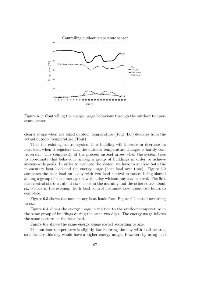
1 2 3 4 5 6 7 8 9 10 11 12 13 14 15 16 17 18 19 20 21 22 23 24

0

10

20

30

40

50

60

Controlling outdoor temperature sensor

Tout

Tout, LC

Trad, supply

Trad, return

Time (h)

Tem

per

atu

re[°

C]

Figure 6.1: Controlling the energy usage behaviour through the outdoor temper-ature sensor

clearly drops when the faked outdoor temperature (Tout, LC) deviates from theactual outdoor temperature (Tout).

That the existing control system in a building will increase or decrease itsheat load when it registers that the outdoor temperature changes is hardly con-troversial. The complexity of the process instead arises when the system triesto coordinate this behaviour among a group of buildings in order to achievesystem-wide goals. In order to evaluate the system we have to analyse both themomentary heat load and the energy usage (heat load over time). Figure 6.2compares the heat load on a day with two load control instances being sharedamong a group of consumer agents with a day without any load control. The firstload control starts at about six o’clock in the morning and the other starts aboutsix o’clock in the evening. Both load control instances take about two hours tocomplete.

Figure 6.3 shows the momentary heat loads from Figure 6.2 sorted accordingto size.

Figure 6.4 shows the energy usage in relation to the outdoor temperature inthe same group of buildings during the same two days. The energy usage followsthe same pattern as the heat load.

Figure 6.5 shows the same energy usage sorted according to size.

The outdoor temperature is slightly lower during the day with load control,so normally this day would have a higher energy usage. However, by using load

87

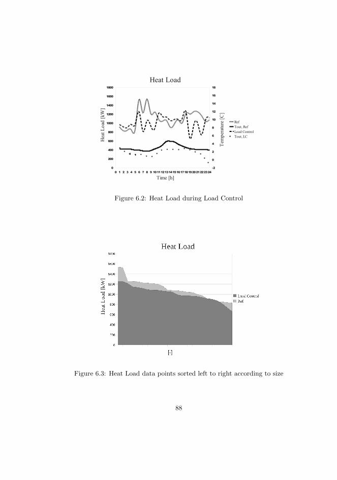
0 1 2 3 4 5 6 7 8 9 101112131415161718192021222324

0

200

400

600

800

1000

1200

1400

1600

1800

-2

0

2

4

6

8

10

12

14

16

18

Heat Load

Ref

Tout, Ref

Load Control

Tout, LC

Time [h]

Hea

tL

oad

[kW

]

Tem

per

ature

[C]

Figure 6.2: Heat Load during Load Control

Figure 6.3: Heat Load data points sorted left to right according to size

88

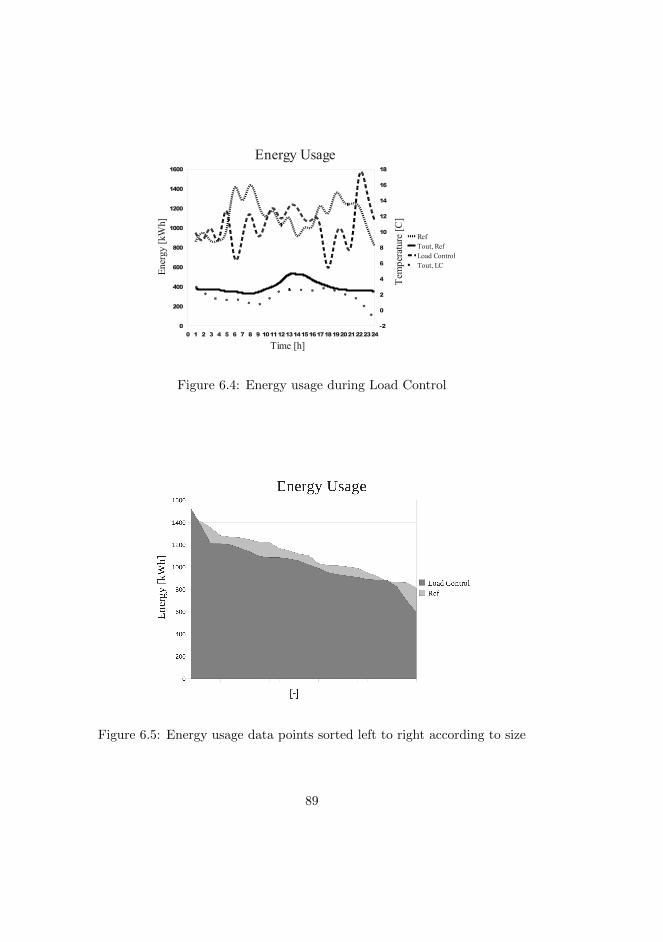
0 1 2 3 4 5 6 7 8 9 101112131415161718192021222324

0

200

400

600

800

1000

1200

1400

1600

-2

0

2

4

6

8

10

12

14

16

18

Energy Usage

Ref

Tout, Ref

Load Control

Tout, LC

Time [h]

Ener

gy

[kW

h]

Tem

per

ature

[C]

Figure 6.4: Energy usage during Load Control

Figure 6.5: Energy usage data points sorted left to right according to size

89

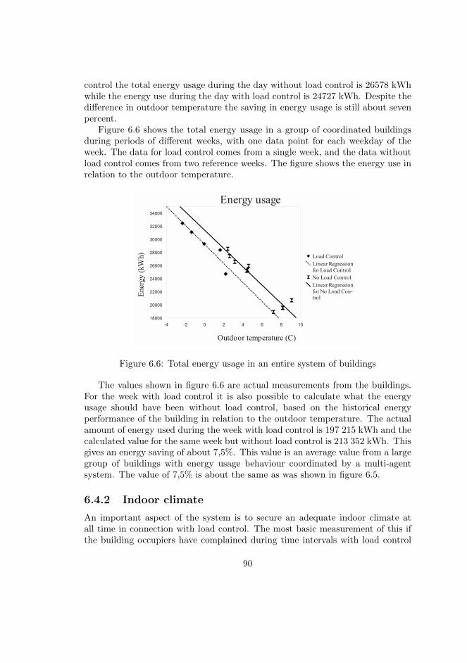
control the total energy usage during the day without load control is 26578 kWhwhile the energy use during the day with load control is 24727 kWh. Despite thedifference in outdoor temperature the saving in energy usage is still about sevenpercent.

Figure 6.6 shows the total energy usage in a group of coordinated buildingsduring periods of different weeks, with one data point for each weekday of theweek. The data for load control comes from a single week, and the data withoutload control comes from two reference weeks. The figure shows the energy use inrelation to the outdoor temperature.

Figure 6.6: Total energy usage in an entire system of buildings

The values shown in figure 6.6 are actual measurements from the buildings.For the week with load control it is also possible to calculate what the energyusage should have been without load control, based on the historical energyperformance of the building in relation to the outdoor temperature. The actualamount of energy used during the week with load control is 197 215 kWh and thecalculated value for the same week but without load control is 213 352 kWh. Thisgives an energy saving of about 7,5%. This value is an average value from a largegroup of buildings with energy usage behaviour coordinated by a multi-agentsystem. The value of 7,5% is about the same as was shown in figure 6.5.

6.4.2 Indoor climate

An important aspect of the system is to secure an adequate indoor climate atall time in connection with load control. The most basic measurement of this ifthe building occupiers have complained during time intervals with load control

90

active. Another way to measure this is to install indoor temperature sensors andsee what happens with the indoor temperature during load control. This wasdone during the project in selected buildings within the multi-agent system.

In practice the system will reduce the heat load in the building, which willinevitable lead to a reduced indoor temperature if allowed to continue uncon-trolled. Each consumer agent is responsible for making sure that this reductionin indoor temperature is small enough for the building occupiers not to notice.There were no complaints during the project that were derived from load control.

The indoor temperature sensors showed no sign of being influenced by loadcontrol. The indoor temperature could vary wildly in individual apartments.This happens all the time and is due to social behaviour such as using electricalappliances, opening windows, or having ten kids over for a birthday party. It wasnot possible to determine when load control was active or not by studying thedata from the indoor temperature sensors.

6.4.3 Available load control ability

In order to evaluate the financial aspects of this type of system it is important forthe energy company to be able to estimate the number of buildings need withinthe multi-agent system. The system-wide operational benefits of the system isdirectly proportional to the number and size of buildings available in relationto the total size of the district heating system. A large building has a greateravailable heat load buffer than a smaller building. Normally it is possible toestimate an average size of buildings within the district heating network, whichcan then be used as a basis for a first estimation of the potential of the system.It is the possible to make a rough estimate of the amount of buildings needed fora given district heating system:

Amount =Heatload

eSig ∗ (Tb − Tout) ∗ LCmax(6.1)

Where Heatload is the amount of heat load [W] that the system should beable to handle, eSig [W/◦C] is the average energy signature in the area, Tb [◦C]isthe outdoor temperature above which a building needs no heating, Tout [◦C] isthe outdoor temperature at time of using load control and LCmax is the maximalshare of the total heat load that the system should be allowed to control. This lastvalue, which is set to 70% for this study, is a general limit that is used in order toensure that the system doesn’t completely shut of the heating, not even duringshorter periods of time. This is a social, rather than physical, consideration,e.g. if someone puts their hand on the radiator it should not be completelycold. This is the maximum value that the system can control of the heat load,

91

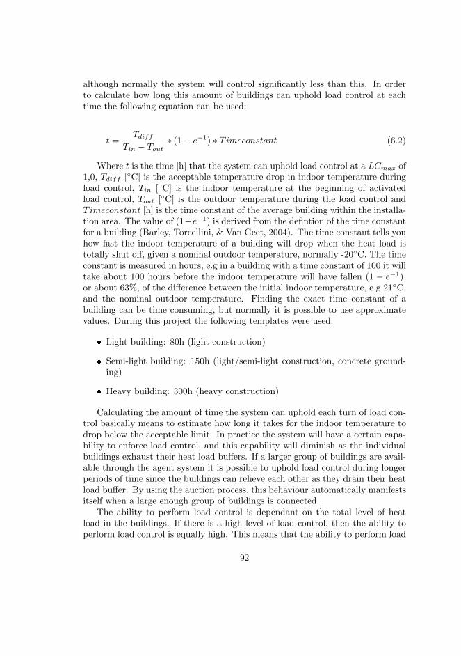
although normally the system will control significantly less than this. In orderto calculate how long this amount of buildings can uphold load control at eachtime the following equation can be used:

t =Tdiff

Tin − Tout∗ (1− e−1) ∗ Timeconstant (6.2)

Where t is the time [h] that the system can uphold load control at a LCmax of1,0, Tdiff [◦C] is the acceptable temperature drop in indoor temperature duringload control, Tin [◦C] is the indoor temperature at the beginning of activatedload control, Tout [◦C] is the outdoor temperature during the load control andTimeconstant [h] is the time constant of the average building within the installa-tion area. The value of (1−e−1) is derived from the defintion of the time constantfor a building (Barley, Torcellini, & Van Geet, 2004). The time constant tells youhow fast the indoor temperature of a building will drop when the heat load istotally shut off, given a nominal outdoor temperature, normally -20◦C. The timeconstant is measured in hours, e.g in a building with a time constant of 100 it willtake about 100 hours before the indoor temperature will have fallen (1 − e−1),or about 63%, of the difference between the initial indoor temperature, e.g 21◦C,and the nominal outdoor temperature. Finding the exact time constant of abuilding can be time consuming, but normally it is possible to use approximatevalues. During this project the following templates were used:

� Light building: 80h (light construction)

� Semi-light building: 150h (light/semi-light construction, concrete ground-ing)

� Heavy building: 300h (heavy construction)

Calculating the amount of time the system can uphold each turn of load con-trol basically means to estimate how long it takes for the indoor temperature todrop below the acceptable limit. In practice the system will have a certain capa-bility to enforce load control, and this capability will diminish as the individualbuildings exhaust their heat load buffers. If a larger group of buildings are avail-able through the agent system it is possible to uphold load control during longerperiods of time since the buildings can relieve each other as they drain their heatload buffer. By using the auction process, this behaviour automatically manifestsitself when a large enough group of buildings is connected.

The ability to perform load control is dependant on the total level of heatload in the buildings. If there is a high level of load control, then the ability toperform load control is equally high. This means that the ability to perform load

92

control increases as the outdoor temperature drops, which in turn means thatthe ability to perform load control is at its highest when the need for it is thegreatest.

6.4.4 Cost-benefit analysis

The largest financial value of lowered heat load is probably when load controlability will help to avoid the need for more peak load production. The amountof heat load that can be moved or lowered is dependant on the characteristics ofboth the production units and the building types available in the district heatingsystem. Normally the need to perform load control only occurs during shorterperiods of time. Normally 30-40% of the heat load has a length of less than 500hours. In most district heating system these loads are produced by oil, electricityor coal. An oil boiler costs about ¿200/kW ($270/kW) to install, which is thefinancial value of the load control system if this installation capability can beavoided. During this project the load control system has lowered heat loadsduring peak hours between 15-20% on average. Avoiding 15% oil based peakload in a 100 MW system is then worth about ¿3M ($4.1M) in saved installationcosts.

Transferring peak load to base load also means lowered variable produc-tion costs. As an example the ability to move from tree oil (cost ¿0,04/kWh($0.055/kWh) including taxes) to bio-fuel (cost about ¿0.02/kWh ($0.027/kWh)including taxes) gives a saving of ¿0.02/kWh ($0.027/kWh). Fortum, who ownsthe district heating network in Stockholm, produces slightly less than 10 000GWh annually. The value of reducing fossil fuel in production is not only afinancial one, but also based on environmental considerations. For security rea-sons it is unlikely that peak load production can be avoided all together, but thebenefits of reducing it as much as possible are numerous.

Load control not only gives the ability to lower the heat load, but also to moveit in time. In this case the buildings can be viewed as the equivalence of the largestorage tanks found in many district heating systems. When using combined heatand power production (CHP) it is normal to optimize the production in relationto the price variation on the spot-price market for power. The spot-price variesduring the day but normally there are price peaks in the morning and evening.The physical process of producing heat and power cannot be separated, but byusing load control it is possible to move the heat load consumption a few hoursin time by controlled pre-heating of the buildings.

93

6.5 Discussion

Performing uninformed local load controls by manipulating the outdoor tem-perature sensor has been shown to be easy enough, although due to aspects ofdynamic (time dependant) indoor climate feedback a certain level of intelligentbehaviour is required when actually implementing energy saving process usingsuch techniques. More interesting and complex problems arise when trying tocoordinate this behaviour from the system wide aspect of the producer, whilestill considering the indoor climate in all the individual buildings. When sortingthe data from figure 6.2 according to size like in figure 6.3 it becomes apparentthat the largest reductions in heat load have been done during the higher peaks.It should be noted that the outdoor temperature during the reference day is +2,9◦C and during the day with load control +1,7 ◦C. No adjustment for this tem-perature difference have been made so the effect of the load control is in realityeven more significant than what is shown in this example.

In order to satisfy the heating need an energy company would normally usea whole range of different production units, with different characteristics andfuels. The production units are started in order by their production costs, whichnormally means that the boilers using oil will only be started during periods ofpeak load with short duration. The absolutely highest peak loads normally havedurations of a few hours. During this project it was noted that in order to lowerthe heat load with 10% the system needed to control the load during no morethan eight hours at most. This is well within the capability of the system studied.

The theoretical optimization normally used in order to find the financiallybest operational strategy for the production units is based on solutions of theEconomic Dispatch Problem (EDP) and the Unit Commitment Problem (UCP)(Koay et al., 2008). By solving the EDP and the UDP an energy companycan find a desired consumption level for each hour during the next few days.This value can then be used as decision data by the multi-agent system in orderto implement load control throughout the day in order to uphold the desiredconsumption level.

6.6 Conclusions

This system consists of distributed units with communication ability that canmeasure sensor data and control the heating system in individual buildings. Theseunits are then controlled by consumer agents which enables the system to coor-dinate the heating behaviour on a system wide scale. By using this system aenergy company can, within the constraints set by indoor climate limits, activelyplan, optimize and control the heat load within a district heating network.

The results show that the system has lowered the total heat load with about

94

20% in connection with the highest peak loads. This value is, however, still farfrom the maximum set limit of LCmax in equation 6.1, i.e. the limit of 70% ofthe heat load which is used in this study. In figure 6.3 it is shown that the largestheat load reductions are done during time intervals with the highest heat load(measured in kW). A district heating network utilizes several differently pricedfuels in order to satisfy the demand, ranging from cheap waste heat and bio fuelsto more expensive alternatives such as oil and electricity. The normal situationin Sweden is that the highest 5-15% of the heat load needs to be satisfied withsome peak load boiler (usually oil)(Constinescu, 2007). Compare this with figure6.3 where the highest heat loads are sorted left to right. It is clear that the agentsystem manages to shed these peak loads in the left-most part of the figure.

By using correct pricing strategies within the district heating network theenergy company wants to achieve transparency so that the costumers understandand act based on the costs of producing the heat. This is a very complex problemand it is not always easy to make the pricing strategy understandable as well astransparent in regards to actual production costs. Also, it is not easy to set aprice according to different conditions since if the customers actually react to thisprice it would change the conditions. This leads to a situation with a variablepricing goal which in practise demands that it is possible to dynamically adjustprices in order for the right production situation to arise. By a correct pricingstrategy it should be simple to give the customers the incentive to invest in loadcontrol equipment. It is, however, important that this equipment is capable ofinteracting on a system-wide scale, since local uninformed load control can domore harm the good from a production perspective. If there is no method forsystem-wide control it is very hard, if not impossible, to use the behaviour ofthe buildings in order to optimize the production. It is also not enough to usestatic predefined lists of buildings to cut heat load in during times of peak loads.Using such predefined lists does not take the dynamics of the indoor climate intoconsideration. It is essential to pay attention to the dynamics of the quality ofservice as well as the production status.

In relation to this discussion it should be noted that it is not suitable tolet human consumers themselves make the dynamic decisions to implement loadcontrol, e.g. by having a wall mounted display showing graphs of energy con-sumption and then expecting people to actually do something when the energyprice is high or the heat/power load is above some threshold. Such schemes havebeen tried several times and the results are normally the same, i.e a consumerwill use the system for a month or two, but will then eventually grow tired ofthe whole thing and stop using it. We believe that the only way to implementsuch systems in the long term is to exchange the human decision maker with anautomated system of some sort.

Besides reducing peak loads the system has also shown a clear ability to lower

95

the energy usage in the participating buildings, without any noticeable differencein the perceived indoor climate. During the project the system showed a energyreduction of about 7,5% during week-long periods. From the perspective of theenergy company and the national economy it is preferable if this reduction inenergy consumption in connection to peak load production instead of during baseload production. Only by using system-wide load control can such a consumerbehaviour be enforced.

The system controls the heat load in individual buildings by manipulatingthe outdoor temperature sensor that the existing control system uses. Each loadcontrol is implemented by faking the outdoor temperature for the existing controlsystem, e.g. if the existing control system during a short period of time is ledto believe that the outdoor temperature is 10 ◦C when in reality it is 5 ◦C, thenthis will lead to a reduction in energy usage during that time. A lowered heatload will obviously led to a lowered indoor temperature sooner or later, which iswhy such load control has to be done within a controlled process. Several indoortemperature sensors were placed within the buildings during the project, in orderto identify lowered temperatures due to load control. Despite of this it has notbeen possible to identify where and if any reduction of the indoor temperature waspresent. It was shown that the indoor temperature within individual apartmentsvaries so much due to social behaviour that the influence of load control is lost inthe noise. In all likelihood the lowered energy usage must have led to a temporaryreduction in the temperature, either in the building body or in the air containedwithin the building, but neither the indoor temperature sensors or any buildingoccupiers have been able to perceive this.

In a heating system where the ventilation has a considerable impact on theindoor climate it is complicated to implement load control by manipulating thesecondary circuit of the heating system. An alternative in these cases is to onlycontrol the heat load in the radiator system and not to include the ventilationhot water in the load control.

During this project we have studied load control within district heating sys-tems, but these system-wide techniques are equally interesting in other energysystems, e.g. power grids or industrial production processes. When, for example,comparing a power grid and a district heating system it is obvious that thereare major differences in the physical process of how energy is transported (waterversus electricity), but on a system-wide scale we believe that there are still manyoverlapping themes.

This project has been a step up from previous small scale experiments andsimulations. It has been shown that the theory holds in practice, and that coor-dinated load control within district heating systems as a technique does indeedwork.

96

6.7 Future work

Early small-scale practical experiments have shown a 4% decrease in energy usagewhen using a multi-agent based system for load control in a district heatingnetwork, and has predicted a theoretical energy saving of about 10% (PaperII). During this study we have shown an energy saving of about 7.5% averagingover groups of buildings. With further tweaking of the behaviour of the systemwe expect this figure to be able to reach the predicted 10%. This might bedone by selecting other techniques for allocating the resources. Using an auctionbased mechanism for this implies that the consumer wishes to spend as little aspossible of its utility, when in reality all agents within the system are cooperatingin achieving the desired load control, i.e a consumer wants to spend as much aspossible of its available buffer but never more than this. This might be interpretedas a suggestion that other methods could be even more successful at distributingthe resources among the agents in such a system, e.g. bargaining schemes orsome sort of distributed/centralized optimization technique.

6.8 Acknowledgements

This work as been a collaboration between NODA Intelligent Systems AB andBlekinge Institute of Technology. The results are based on a project financed byNODA Intelligent Systems AB, Fortum Varme AB, Malareenergi AB, TekniskaVerken i Linkoping AB and The Swedish District Heating Association.

97

98

Chapter 7

Paper VI - Heat loadreductions and their effecton energy consumption

In this paper we investigate the consequences of using temporary heat load reduc-tions on consumer substations, from the perspective of the individual consumeras well as the district heating company. The reason for using such reductions arenormally to save energy at the consumer side, but the ability to control the heatload also lie at the core of more complex control processes such as Demand SideManagement (DMS) and Load Control (LC) within district heating systems. Thepurpose of this paper is to study the way different types of heat load reductionsimpact on the energy usage as well as on the indoor climate in the individualbuildings. We have performed a series of experiments in which we have equippedmulti-apartment buildings with wireless indoor temperature sensors and a noveltype of load control equipment, which gives us the ability to perform remotely su-pervised and coordinated heat load reductions among these buildings. The resultsshow that a substantial lowering of the heat load and energy usage during periodsof reductions is possible without jeopardizing the indoor climate, although we showthat there are differences in the implications when considering different types ofheat load reductions.

7.1 Introduction

The main purpose of this paper is to investigate the consequences of using tem-porary heat load reductions on consumer substations within a district heating

99

network. The most common way to perform temporary heat load reductions isto use night time set-back, i.e. to lower the wanted indoor temperature duringnight time while social activity is expected to be low. Emerging technologies likeDemand Side Management (DMS) and Load Control (LC) also use temporaryheat load reductions in order to accomplish system wide control strategies, al-though the characteristic of these head load reductions differ significantly fromnight time set-back.

In the context of this study we regard a heat load reduction to be the wholeprocess from the initial change of heat load, through the return to normal heatload, and until no evidence of the heat load reduction can be noticed in thedynamics of the building energy balance. This definition is based on the factthat the heat load reduction will continue to exert an influence on the buildingsthermal buffer for some time even after the heat load reduction in itself is ended.The length of this interval is specific to each building and is related to the thermalinertia of the building in question.

In this paper we study the consequences of using different types of heat loadreductions, and try to analyse the way the thermal buffer of the building isaffected along with the actual heat load and energy usage from both a local and aglobal perspective. We study the performance of both long low-intensity heat loadreductions (e.g. night time set-back) as well as short high-intensity reductions(e.g. those frequently used in DMS schemes). The use of night time set-back hasreceived some attention in previous works, e.g (Bjorsell, n.d.), and the possibilitiesto use the building as a heat buffer has been evaluated (Olsson Ingvarsson &Werner, 2008), but heat load reductions such as those used in DSM and LC haveto the knowledge of the authors not been thoroughly investigated.

7.1.1 Night time set-back

Night time set-back means to lower the wanted indoor temperature during nighttime, with the purpose of saving energy through reduced heat losses due to de-creased difference between indoor and outdoor temperature. This is the mostcommon way to perform temporary heat load reductions, and many commercialcontrol systems support this feature. This is normally done by a parallel displace-ment of the heat control curve during night hours. During night time set-back thewanted indoor temperature will be set to one, or a few, degrees lower than duringnormal operations. There is, however, an ongoing debate on whether night timeset-back actually gives an energy saving or not (Lindkvist & Wallentun, 2004),and most practical implementations of night time set-back suffer from morningpeak loads when the control system returns to the original operational level. Still,almost all control equipment companies sell equipment that facilitates the use ofnight time set-back, and the use of this technique is widespread.

100

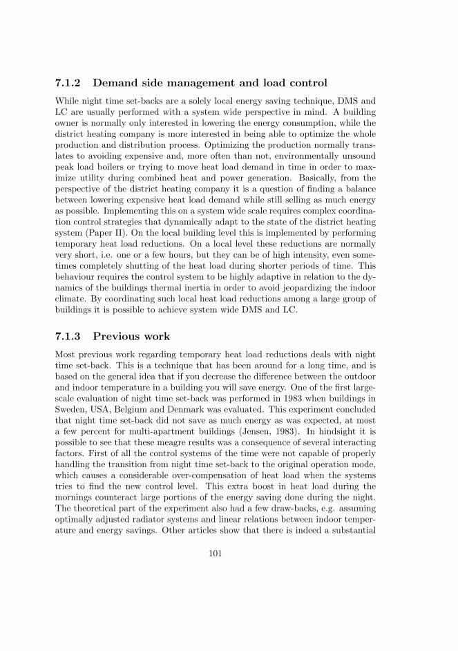
7.1.2 Demand side management and load control

While night time set-backs are a solely local energy saving technique, DMS andLC are usually performed with a system wide perspective in mind. A buildingowner is normally only interested in lowering the energy consumption, while thedistrict heating company is more interested in being able to optimize the wholeproduction and distribution process. Optimizing the production normally trans-lates to avoiding expensive and, more often than not, environmentally unsoundpeak load boilers or trying to move heat load demand in time in order to max-imize utility during combined heat and power generation. Basically, from theperspective of the district heating company it is a question of finding a balancebetween lowering expensive heat load demand while still selling as much energyas possible. Implementing this on a system wide scale requires complex coordina-tion control strategies that dynamically adapt to the state of the district heatingsystem (Paper II). On the local building level this is implemented by performingtemporary heat load reductions. On a local level these reductions are normallyvery short, i.e. one or a few hours, but they can be of high intensity, even some-times completely shutting of the heat load during shorter periods of time. Thisbehaviour requires the control system to be highly adaptive in relation to the dy-namics of the buildings thermal inertia in order to avoid jeopardizing the indoorclimate. By coordinating such local heat load reductions among a large group ofbuildings it is possible to achieve system wide DMS and LC.

7.1.3 Previous work

Most previous work regarding temporary heat load reductions deals with nighttime set-back. This is a technique that has been around for a long time, and isbased on the general idea that if you decrease the difference between the outdoorand indoor temperature in a building you will save energy. One of the first large-scale evaluation of night time set-back was performed in 1983 when buildings inSweden, USA, Belgium and Denmark was evaluated. This experiment concludedthat night time set-back did not save as much energy as was expected, at mosta few percent for multi-apartment buildings (Jensen, 1983). In hindsight it ispossible to see that these meagre results was a consequence of several interactingfactors. First of all the control systems of the time were not capable of properlyhandling the transition from night time set-back to the original operation mode,which causes a considerable over-compensation of heat load when the systemstries to find the new control level. This extra boost in heat load during themornings counteract large portions of the energy saving done during the night.The theoretical part of the experiment also had a few draw-backs, e.g. assumingoptimally adjusted radiator systems and linear relations between indoor temper-ature and energy savings. Other articles show that there is indeed a substantial

101

level of energy saving to be found by controlling the local heat load (Morris,Braun, & Treado, 1994).

Most of the previous work done on the subject is based on simulated results.This is expected since the dynamic thermal processes within a building are ex-tremely complex and it is not surprising that comparisons between measurementsand calculations sometimes show large discrepancies. It is noted that most cal-culations are dependant on variables that cannot be measured and verified, andthat the the building time constant is really not a constant (Isfalt & Broms,1992).

7.2 Experimental method

In order to study the effects of temporary heat load reductions we equippeda building with several wireless temperature sensors in order to measure thefluctuations in indoor temperature. The building in questions is an office buildingwith semi-light thermal characteristics (light construct with concrete slab) and atime constant of about 150 hours (Ruud, 2009). The indoor temperature sensorswere placed on different locations within the building in order to get a goodoverview of the thermal behaviour of the indoor climate. In addition to theexisting outdoor temperature sensor an extra wireless sensor was also placed onthe outside of the building. Unlike the existing outdoor temperature sensor thewireless one was placed in a position were it was fully exposed to any possiblesunshine. This gave us an extra indication of the impact of free heating throughwindow areas, even though we did not have any ability to measure the actualsolar irradiance.

In order to control the district heating consumer station we connected a loadcontrol platform for system wide LC and DSM (Paper VIII). This platform isbased on a novel form of hardware and software which enables us to managethe heat load of the substation without any major alterations or any damage onthe existing hardware. The software system is based on the open source Linuxoperating system and is equipped with an application programming interface(API) for I/O. This makes it easy to apply additional sensors, e.g. for measuringthe forward and return temperatures of the radiator system. The platform alsofeatures connections to a database system which enables real-time logging andanalyse of sensor data. The actual heat load reductions are implemented bysupplying the existing control system with adjusted outdoor temperatures, whichgives us the ability to manage the behaviour of the heat load without exchangingany existing hardware. This adjusted outdoor temperature can be managed witha resolution of at most 60 seconds. The computer platform uses either Ethernetor GPRS modems to communicate with the database. In our case we used theexisting Internet access in the building. In addition to this primary experimental

102

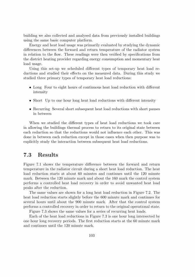
building we also collected and analysed data from previously installed buildingsusing the same basic computer platform.

Energy and heat load usage was primarily evaluated by studying the dynamicdifferences between the forward and return temperature of the radiator systemin relation to the flow. These readings were then verified by specifications fromthe district heating provider regarding energy consumption and momentary heatload usage.

Using this set-up we scheduled different types of temporary heat load re-ductions and studied their effects on the measured data. During this study westudied three primary types of temporary heat load reductions:

� Long Four to eight hours of continuous heat load reduction with differentintensity

� Short Up to one hour long heat load reductions with different intensity

� Recurring Several short subsequent heat load reductions with short pausesin between

When we studied the different types of heat load reductions we took carein allowing the buildings thermal process to return to its original state betweeneach reduction so that the reductions would not influence each other. This wasdone in between each reduction except in those cases when then purpose was toexplicitly study the interaction between subsequent heat load reductions.

7.3 Results

Figure 7.1 shows the temperature difference between the forward and returntemperature in the radiator circuit during a short heat load reduction. The heatload reduction starts at about 60 minutes and continues until the 120 minutemark. Between the 120 minute mark and about the 160 mark the control systemperforms a controlled heat load recovery in order to avoid unwanted heat loadpeaks after the reduction.

The same values are shown for a long heat load reduction in Figure 7.2. Theheat load reduction starts slightly before the 600 minute mark and continues forseveral hours until about the 900 minute mark. After that the control systemperforms a controlled recovery in order to return to the original operational state.

Figure 7.3 shows the same values for a series of recurring heat loads.Each of the heat load reductions in Figure 7.3 is one hour long intersected by

one hour long recovery periods. The first reduction starts at the 60 minute markand continues until the 120 minute mark.

103

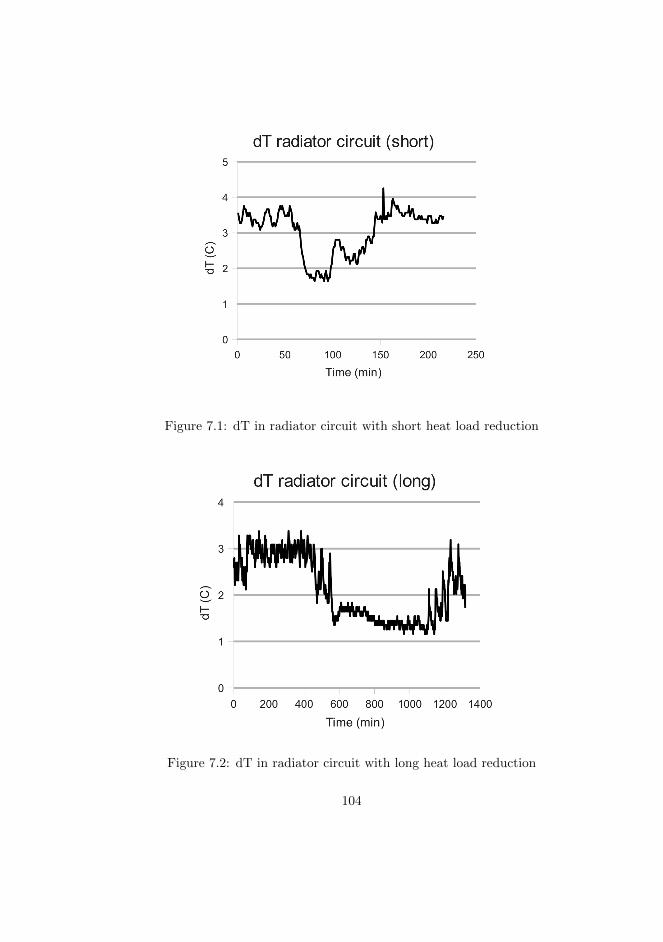
Figure 7.1: dT in radiator circuit with short heat load reduction

Figure 7.2: dT in radiator circuit with long heat load reduction

104

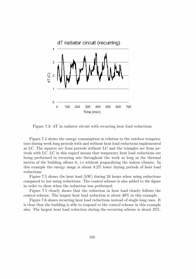
Figure 7.3: dT in radiator circuit with recurring heat load reductions

Figure 7.4 shows the energy consumption in relation to the outdoor tempera-ture during week long periods with and without heat load reductions implementedas LC. The squares are from periods without LC and the triangles are from pe-riods with LC. LC in this regard means that temporary heat load reductions arebeing performed in recurring sets throughout the week as long as the thermalinertia of the building allows it, i.e without jeopardizing the indoor climate. Inthis example the energy usage is about 8.2% lower during periods of heat loadreductions.

Figure 7.5 shows the heat load (kW) during 24 hours when using reductionscompared to not using reductions. The control scheme is also added to the figurein order to show when the reduction was performed.

Figure 7.5 clearly shows that the reduction in heat load closely follows thecontrol scheme. The largest heat load reduction is about 30% in this example.

Figure 7.6 shows recurring heat load reductions instead of single long ones. Itis clear that the building is able to respond to the control scheme in this examplealso. The largest heat load reduction during the recurring scheme is about 25%.

105

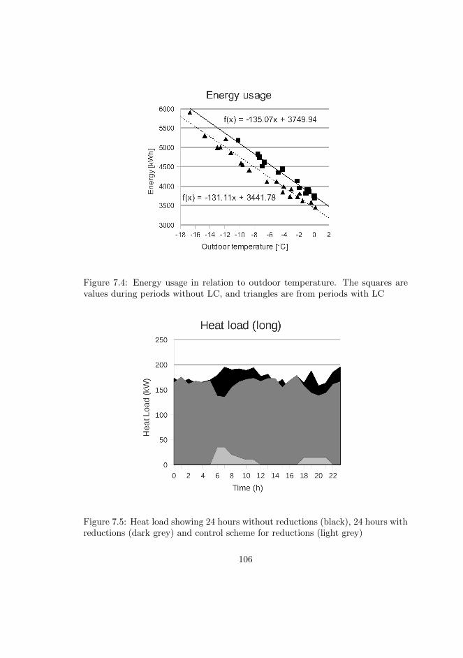
Figure 7.4: Energy usage in relation to outdoor temperature. The squares arevalues during periods without LC, and triangles are from periods with LC

Figure 7.5: Heat load showing 24 hours without reductions (black), 24 hours withreductions (dark grey) and control scheme for reductions (light grey)

106

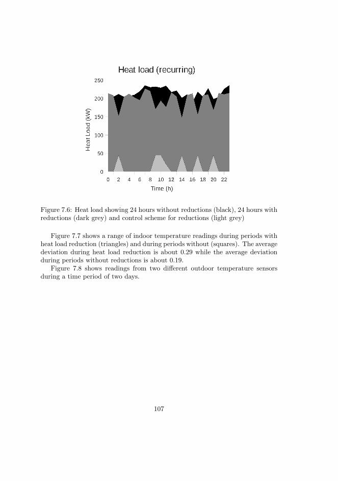
Figure 7.6: Heat load showing 24 hours without reductions (black), 24 hours withreductions (dark grey) and control scheme for reductions (light grey)

Figure 7.7 shows a range of indoor temperature readings during periods withheat load reduction (triangles) and during periods without (squares). The averagedeviation during heat load reduction is about 0.29 while the average deviationduring periods without reductions is about 0.19.

Figure 7.8 shows readings from two different outdoor temperature sensorsduring a time period of two days.

107

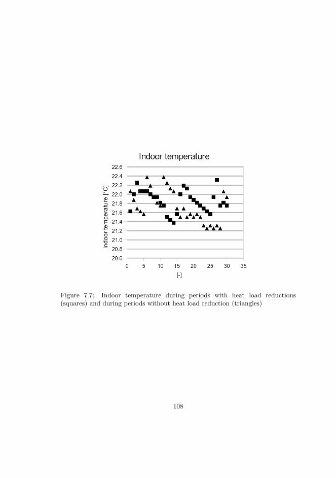
Figure 7.7: Indoor temperature during periods with heat load reductions(squares) and during periods without heat load reduction (triangles)

108

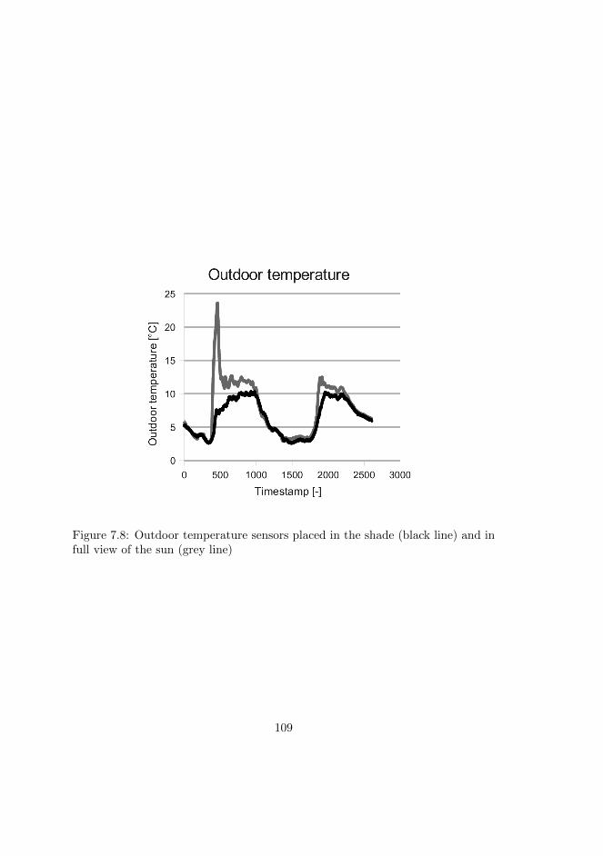
Figure 7.8: Outdoor temperature sensors placed in the shade (black line) and infull view of the sun (grey line)

109

The graph shows the outdoor temperature sensor which is connected to theactual consumer sub-station in the building (black line). Normally these sensorsare placed somewhat in the shadow to avoid large fluctuations due to solar radi-ation. We added another temperature sensor (grey line) in order to estimate theimpact of this solar radiation. Hence this sensor was placed in full view of thesun. The first day was sunny during most of the morning until midday, while thesecond day was more cloudy.

7.4 Discussion

When dealing with temporary heat load reductions it is important to include thewhole process of the reduction. This also includes what happens after the actualheat load reduction has been performed. For example, when just restoring thewanted control level after a long reduction, e.g night time set-back, the forwardflow temperature in the radiator system will rise much faster than the return flowtemperature. This causes a substantial, although temporary, heat load increasein the radiator system which negates large portions of the energy saving doneduring the actual reduction. Apart from decreasing the local net energy savingthis behaviour is also less than desired from a system wide perspective, sinceit causes massive heat load peaks if done in many buildings simultaneously, e.g.contributing to morning peak loads. In order to avoid this it is important to factorin the whole process of the reduction, and make sure that the control systemproperly handles the transition from the reduction level to the original level. Theinability among most commercially available control systems to properly handlethis over-compensation is most likely contributing a great deal to the lingeringcontroversy whether night time set-back actually gives an energy saving or not.

It is important to realize that the definition of an acceptable indoor temper-ature is not about having the indoor temperature at a certain precise level atall time, but rather to have it within a certain, socially acceptable, temperatureinterval at all time. This has been discussed at great length in previous work(Isfalt & Broms, 1992). The general idea is that a greater temperature intervalwill lower the need of additional heating from the radiator system, by coordi-nating the thermal inertia of the building with freely available heat, e.g. heatfrom sunlight or electrical appliances, to balance the heating need. This notionis supported by our results as we have shown that the thermal inertia of evena small or medium sized multi-apartment building is considerable. How peopleperceive the indoor climate is dependant not only on the actual indoor temper-ature itself but also on other factors like air quality, individual metabolism andbehaviour, radiation temperature and air movement. In relation to this it canbe noted that previous work have shown that about five percent of any group ofpeople will always be unsatisfied by the indoor climate (Skoog, 2005), and that

110

it is not possible to create a perfect climate that will make everyone happy.

7.5 Conclusions

There is an ongoing debate whether night time set-backs lead to an energy re-duction or not. Results from this study clearly show an energy saving in relationto heat load reductions, although this assumes that the control system is able tosmoothly handle the transition from reduction to normal operation. The resultsshowing energy saving is evaluated in relation to the total energy usage whichalso includes tap-water usage. Normally this is estimated to about 30% of thetotal energy use in a multi-apartment building.

In prior studies of temporary heat load reductions the focus has been onthe fluctuations in the indoor temperature as a way of evaluating the energysaving (Jensen, 1983). This idea is based on the widespread notion that anyenergy saving is linearly proportional to the temperature difference between theindoor and outdoor temperature. This model might be true in a steady statesimulation where the temperature difference is assumed to have had time topermeate the air mass as well as the entire building structure, but it is obviouslyinadequate in a dynamic situation. We have instead focused on the heat load andenergy usage directly, i.e. the difference between forward and return temperaturein relation to the flow within the radiator circuit. In most of the buildingsevaluated there has been a considerable reduction of energy consumption withoutany noticeable change in indoor temperature. The reason that there does not needto be a measurable change of the indoor temperature is due to the dynamics ofthe thermal inertia of the building, e.g. the time constant of a building is not aconstant (Isfalt & Broms, 1992). This aspect comes into play when using veryshort heat load reductions, at most one or a few hours long. During this firstpart of the reduction it is mainly the actual air mass that is influencing theindoor temperature drop since this body has a low resistance to change, i.e. theshort time constant (Norberg, 1990). If the heat load reduction is prolonged, likeduring a night time set-back, the building mass will start to interact with theair mass and thus stabilizing the continuing temperature drop, i.e. the long timeconstant (Norberg, 1990).

The influence of external and internal free heat is large enough that whenthese heat sources interact with other parts of the thermal process it hides shorterheat load reductions in the ambient temperature. This can be seen in Figure 7.7where it is shown that although the average indoor temperature is not noticeablyaffected there is still a somewhat larger deviation in the indoor temperature whichimplies that there is indeed a higher level of temperature flux within the air massand that this is triggered by the heat load reductions. The control policies usedduring this work obviously set a high bar for the control system to handle, but as

111

the average hardware develops it should be possible to implement such techniqueson a larger scale.

Figure 7.8 gives a another clear indication of just how substantial such sourcesof free energy can be. This extra heating due to solar radiation through thewindows directly interacts with the mass of air inside the building, thus raisingthe temperature. In addition to being able to help save energy usage in a buildingtemporary heat load reductions also form the backbone of DSM and LC, in whichthe goal is to manage the heat load (kW) rather than the energy usage (kWh).

7.6 Future work

In the future we plan to further develop models in order to dynamically esti-mate the temperature flux within buildings and develop theoretical and practicalinterfaces for incorporating this data dynamically into the control systems.

7.7 Acknowledgement

This work has been financed by Blekinge Institute of Technology and NODAIntelligent Systems AB.

112

Chapter 8

Paper VII - Combined heatand power generation usingsmart heat grid

Combined heat and power (CHP) generation is often used when building newdistrict heating production. CHP makes it possible to simultaneously produceelectricity and heat, thus maximizing the energy efficiency of the primary fuel.The heat is used in the connected district heating system while the electricity issold on the local power market. In a CHP plant it is not possible to separate thephysical process of producing heat and electricity, which may cause suboptimalbehaviour when high spot prices for power do not coincide with high heat loaddemand. This paper presents the design and implementation of a system whichmakes it possible to control the heat load demand in a district heating network inorder to optimize the CHP production. By using artificial intelligence technologyin order to automate the run-time coordination of the thermal inertia in a largeamount of buildings, it is possible to achieve the same operational benefits as usinga large storage tank, albeit at a substantially less investment and operational cost.The system continuously considers the climate in each participating building inorder to dynamically ensure that only the best suited buildings at any given timeare actively participating in load control. Based on the dynamic indoor climatein each individual building the system automatically controls and coordinates thecharging and discharging of the buildings thermal buffer without affecting thequality of service. This paper describes the overall function of the system andpresents an algorithm for coordinating the thermal buffer of a large amount ofbuildings in relation to heat load demand and spot price projections. Operational

113

data from a small district heating system in Sweden is used in order to evaluatethe financial and environmental impact of using this technology. The results showsubstantial benefits of performing such load control during times of high spot pricevolatility.

8.1 Introduction

In a district heating system (DHS) one or several production units distributeheated water or steam throughout a pipe network. Buildings are connected tothis network either directly or by heat exchangers. This delivered heat can thenbe used for a multitude of purposes within the building, e.g. radiator subsystems,hot tap water or heating of ventilation air. The basic concept with centralizedproduction units is normally environmentally and financially sound, since suchfacilities can easier incorporate large scale energy efficiency schemes. Districtheating is most common in northern and eastern parts of Europe including Russiaand other former Soviet countries, although the concept is utilized around theworld and is gaining an increasing acceptance on markets throughout Asia andNorth America (Constinescu, 2007).

Any type of production can be used in a DHS, as long as it is able to heatthe water to the desired level. This flexibility allows a wide range of differentproduction solutions, such as industrial waste heat, geothermal heat, biomass,fossil fuel boilers and nuclear powered heating. In many DHS a cogeneration plantis also added to the system. This provides the possibility to produce electricalpower in parallel with the heat production. Such combined heat and power(CHP) systems typically have a very high level of energy efficiency compared tostand-alone thermal production plants (Horlock, 2008). In a CHP plant wateris heated to steam, which is then led into a turbine which in turn transformsthe kinetic energy to electricity in a generator. The steam is then cooled bytransferring its heat to the return water in the district heating system, which inturn is distributed throughout the DHS.

The electricity produced by the generator is normally sold on the power mar-ket. In northern Europe the power market is run by Nord Pool Spot, whichwas the worlds first market for trading power. Nord Pool Spot provides a mar-ket for buying and selling power in Sweden, Finland, Denmark and Norway aswell as in Estonia, Germany and Great Britain. In 2010 the total power tradedthrough Nord Pool Spot amounted to 310 TWh, which correlates to a monetaryvalue of about EUR 18 billion (NordPoolSpot, 2012). Since the power marketis deregulated it is subject to basic market characteristics such as the balancebetween supply and demand. Since energy in the form of electricity is by naturequite hard to store, the electricity has to be made available at the same time asthere is a need for it. And since both this demand and the available supply vary

114

throughout the day, the price for electricity will obviously also vary throughoutthe day. On Nord Pool Spot power is traded based on hourly market prices.These spot prices are traded one day in advance, and are then published on thesame day at 14.00 CET as a set of 24 spot prices, each correlating to an hour thefollowing day. There is also an intraday market at Nord Pool Spot. The intradaymarket acts as a balancing tool between supply and demand in real time. Priceson the day-ahead market can vary quite a lot during a 24 hour period, and situ-ations where the highest spot price for the day is twice that of the lowest is notuncommon. At the intraday market prices can be even more volatile.

These price changes obviously make it financially sound for the individual en-ergy companies to try and match their production with the highest spot prices. Ina DHS/CHP system the physical act of producing electricity cannot be separatedin time from heat production. However, if the heat can be stored in preparationfor the heat load demand, it is possible to optimize the CHP process in relationto power spot prices. By using large heat water storage tanks it is possible todo this, by charging the storage tanks while the power spot prices are high re-spectively discharging them when the heat load demand rises in the buildings.However, such storage tanks are expensive to build and maintain, and their op-erational characteristics are inflexible. This paper presents an alternative way tomanage heat production in relation to the spot price market. By using its ther-mal inertia it is possible to charge and discharge a building with slight amountsof heat energy without affecting the perceived indoor climate (C. Johansson &Wernstedt, 2010b) (Olsson Ingvarsson & Werner, 2008). If this behaviour is co-ordinated among a sufficiently large group of buildings the amount of energycontrolled is comparable to any storage tank, albeit at a much lower installationand maintenance cost. Such a system also has the added benefit of having a moreflexible operational behaviour than a storage tank, since the heat load changesin an individual building are only limited in time by the speed of the connectingvalve.

Controlling the heat load in buildings is known as demand side management(DSM) and can be implemented either by passive tools, e.g. design of pricelists, or by active tools such as direct load control (Sipila & Karkkainen, 2000)(Wernstedt, Davidsson, & Johansson, 2007). The heat load demand in a buildingis basically related to two different driving forces; a) the heating demand and b)the hot tap water demand. The heating demand closely follows the changes inoutdoor temperature while the tap water demand is caused by social behaviour.Although social behaviour does display predictable patterns from a macroscopicpoint of view, the tap water usage cannot be used in relation to heat load control,since the tap water system needs a continuous heat load level in order to avoidLegionella growth. Also the tap water system is subject to direct feedback re-garding quality of service (QoS) if the heat load is changed, e.g. a person taking

115

a shower will instantaneously identify a drop in the tap water temperature. Theheat balance of the building itself however, is a physical process characterised bya more slow-moving nature. If the heat load for the heating system is removedit will normally take several hours before any person in the building will noticeany change (Olsson Ingvarsson & Werner, 2008). This process is even more inertwhen only a subset of the heat load is manipulated.

Normally the heating control system of a building will control the forwardtemperature in the radiator system based solely on the outdoor temperature.Active load control basically equates to temporarily diverting from this. This isdone by controlling the heat load demand, and thus the forward temperature inthe radiator system, based on some other control signal. The scheme presented inthis paper is initiated by a system wide heat load analysis which is synchronizedwith spot price projections. Active load control is then performed in order toimplement the calculated heat load demand strategy while maintaining sufficientlevels of QoS.

The paper starts off by introducing related and previous work concerning thesubject. In section three heat load storage and load control in buildings is dis-cussed in more detail. Section four details an optimization model for correlatingspot price and heat load demand. Section five describes how the load controlsystem is designed while the process of evaluating its behaviour is described insection six. The results are presented in section seven, while section eight dis-cusses the system and the results. The paper is finalized in section eight and ninewith conclusions and future work.

8.2 Related work

The basic prerequisite ability to use the thermal mass of buildings as heat storagefacilities has been thoroughly investigated in previous work. It has been shownthat substantial amounts of energy can be saved in relation to both heatingand cooling demand, even just by considering passive use of a buildings ther-mal mass during the architectural design phase (Hietmaki, Kuoppala, Kalema, &Taivalantti, 2003) (Concrete for Energy Efficient Buildings The benefits of ther-mal mass, 2007). By actively using the thermal inertia within building structuresit is possible to equate this to the operational behaviour of large storage tanks(Olsson Ingvarsson & Werner, 2008).

Such active load control has been studied in relation to building thermal mass,where the validity of the concept is proved through practical experimentation.Such operational load control systems have been evaluated since the eighties(Osterlind, 1982). This early system used the electricity network in order tocommunicate load control commands to each building. This was a one-way com-munication set-up which prevented the system from considering aspects relating

116

to QoS, which meant that the system was controlled without any feedback fromthe individual buildings. It is not until the last decade that technological progressin relation to communication and processing has become sufficiently adaptableand reasonably priced to warrant any large scale installations (C. Johansson,Wernstedt, & Davidsson, 2010b). In particular the development of inexpen-sive and robust infrastructures for communication has been a pivotal aspect ofthis development, and previous work has shown how different levels of availablecommunication affect the efficiency of active load control in operational settings(C. Johansson, Wernstedt, & Davidsson, 2010a). Although the realization thatreliable two-way communication was of outmost importance is evident even inthe earlier works (Osterlind, 1990).

The concept of DSM quality filters was proposed in a previous paper as away of managing the relation between energy companies increasing demand forenvironmentally and financially optimized operational planning and customersdemand of robust and continuous QoS (Wernstedt & Johansson, 2008). Main-taining a sufficient level of QoS is paramount for any load control scheme. Systemwide active load control is dependent on the coordination of heat load demandin a large group of buildings, and normally the end-customers occupying thesebuildings are not sympathetic to overly volatile heat deliveries.

8.3 Load control in buildings

Normally the control system in a building will manage the heating by continu-ously measuring the outdoor temperature and adjusting the temperature of thesecondary heat system accordingly. In most cases this control is performed bysome sort of PI or PID feedback mechanism (KJ & T, 1995). In order to performactive load control in the building this normal control has to be overridden dur-ing each load control instance. This is normally done by offsetting the outdoortemperature signal to some degree, either by predefined internal processes in theexisting control system software, or by external manipulation of the signal fromthe outdoor temperature sensor. Many existing control systems attenuate thesignal from the outdoor temperature sensor, in order to avoid volatility in theresulting control signal due to rapid changes in outdoor temperature. Such at-tenuation should preferably be minimized in systems aimed at performing activeload control, since they cause the system to react slower than is necessary.

The QoS needs to be maintained at all times in each individual buildingparticipating in the load control scheme. One obvious solution for this is to useindoor temperature sensors which give continuous feedback to the system. Manysolutions for such temperature measurements exist, and lately solutions based onwireless technology have also become more widely available. The main problemwith wired solutions in this regard in the cost of installing such systems, since

117

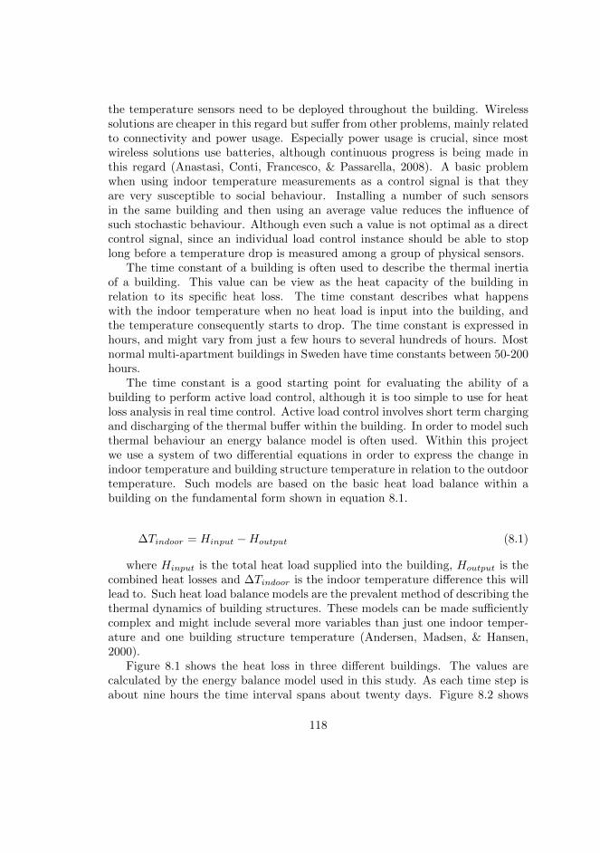
the temperature sensors need to be deployed throughout the building. Wirelesssolutions are cheaper in this regard but suffer from other problems, mainly relatedto connectivity and power usage. Especially power usage is crucial, since mostwireless solutions use batteries, although continuous progress is being made inthis regard (Anastasi, Conti, Francesco, & Passarella, 2008). A basic problemwhen using indoor temperature measurements as a control signal is that theyare very susceptible to social behaviour. Installing a number of such sensorsin the same building and then using an average value reduces the influence ofsuch stochastic behaviour. Although even such a value is not optimal as a directcontrol signal, since an individual load control instance should be able to stoplong before a temperature drop is measured among a group of physical sensors.

The time constant of a building is often used to describe the thermal inertiaof a building. This value can be view as the heat capacity of the building inrelation to its specific heat loss. The time constant describes what happenswith the indoor temperature when no heat load is input into the building, andthe temperature consequently starts to drop. The time constant is expressed inhours, and might vary from just a few hours to several hundreds of hours. Mostnormal multi-apartment buildings in Sweden have time constants between 50-200hours.

The time constant is a good starting point for evaluating the ability of abuilding to perform active load control, although it is too simple to use for heatloss analysis in real time control. Active load control involves short term chargingand discharging of the thermal buffer within the building. In order to model suchthermal behaviour an energy balance model is often used. Within this projectwe use a system of two differential equations in order to express the change inindoor temperature and building structure temperature in relation to the outdoortemperature. Such models are based on the basic heat load balance within abuilding on the fundamental form shown in equation 8.1.

∆Tindoor = Hinput −Houtput (8.1)

where Hinput is the total heat load supplied into the building, Houtput is thecombined heat losses and ∆Tindoor is the indoor temperature difference this willlead to. Such heat load balance models are the prevalent method of describing thethermal dynamics of building structures. These models can be made sufficientlycomplex and might include several more variables than just one indoor temper-ature and one building structure temperature (Andersen, Madsen, & Hansen,2000).

Figure 8.1 shows the heat loss in three different buildings. The values arecalculated by the energy balance model used in this study. As each time step isabout nine hours the time interval spans about twenty days. Figure 8.2 shows

118

Figure 8.1: Heat loss in buildings with three different time constants. 80 hours(continuous), 150 hours (dashed) and 250 hours (dotted). The time scale is innine hour increments.

data generated by the energy balance model compared to actual measurementdata from a real building. The building in question is a very large school buildingwith a considerable time constant of about 380 hours. During one weekendthe building heating system suffered a total breakdown, which enabled us tomeasure the temperature drop during the time it took to repair the heatingsystem (Wernstedt & Johansson, 2009). The repair time is slightly less than 36hours, which is the time span shown in Figure 8.2. Since this is only a smallpart of the time constant of the building the graph does not display the fulllogarithmic behaviour present in the previous figure.

In order to ensure sufficient levels of QoS the proposed systems uses thecombination of an energy balance model and physical indoor temperature sensors.Having access to actual measured temperature data is invaluable in order to gainacceptance for active load control among building owners and residents.

8.4 Heat load synchronization

In order to synchronize future heat load and spot price peaks, it is necessaryto have projections of both these values. The spot prices on the Nord PoolSpot power market is published one day ahead so this data is freely available.A heat load projection can be modelled based on weather forecasts. Since theprojection is short term, in this case one day ahead, and the only variable usedis outdoor temperature the weather forecasts are sufficiently accurate. The heatload projections are then arranged in accordance with the spot price, in this casean array of 24 values correlating to system wide heat load demand for each hour

119

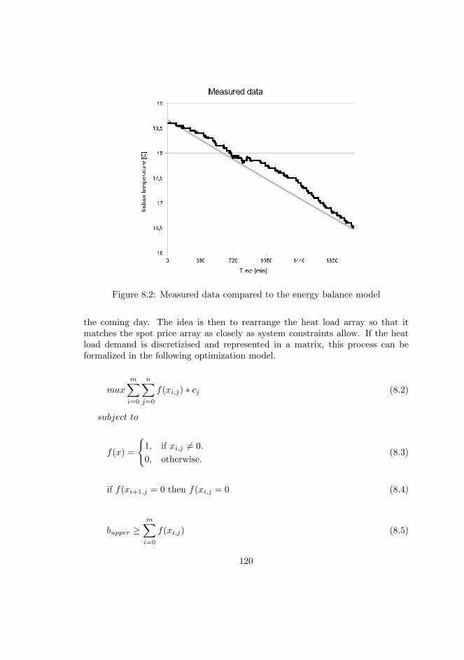
Figure 8.2: Measured data compared to the energy balance model

the coming day. The idea is then to rearrange the heat load array so that itmatches the spot price array as closely as system constraints allow. If the heatload demand is discretizised and represented in a matrix, this process can beformalized in the following optimization model.

max

m∑i=0

n∑j=0

f(xi,j) ∗ cj (8.2)

subject to

f(x) =

{1, if xi,j 6= 0.

0, otherwise.(8.3)

if f(xi+1,j = 0 then f(xi,j = 0 (8.4)

bupper ≥m∑i=0

f(xi,j) (8.5)

120

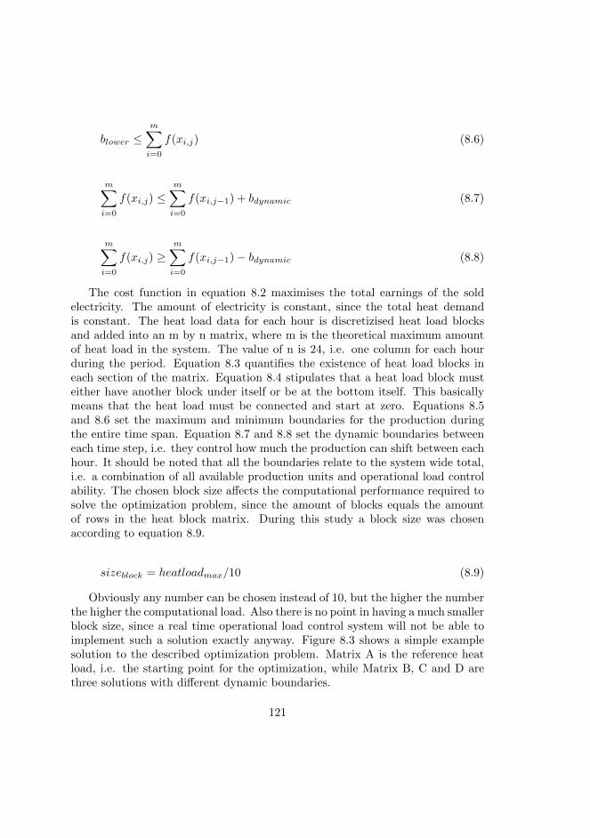
blower ≤m∑i=0

f(xi,j) (8.6)

m∑i=0

f(xi,j) ≤m∑i=0

f(xi,j−1) + bdynamic (8.7)

m∑i=0

f(xi,j) ≥m∑i=0

f(xi,j−1)− bdynamic (8.8)

The cost function in equation 8.2 maximises the total earnings of the soldelectricity. The amount of electricity is constant, since the total heat demandis constant. The heat load data for each hour is discretizised heat load blocksand added into an m by n matrix, where m is the theoretical maximum amountof heat load in the system. The value of n is 24, i.e. one column for each hourduring the period. Equation 8.3 quantifies the existence of heat load blocks ineach section of the matrix. Equation 8.4 stipulates that a heat load block musteither have another block under itself or be at the bottom itself. This basicallymeans that the heat load must be connected and start at zero. Equations 8.5and 8.6 set the maximum and minimum boundaries for the production duringthe entire time span. Equation 8.7 and 8.8 set the dynamic boundaries betweeneach time step, i.e. they control how much the production can shift between eachhour. It should be noted that all the boundaries relate to the system wide total,i.e. a combination of all available production units and operational load controlability. The chosen block size affects the computational performance required tosolve the optimization problem, since the amount of blocks equals the amountof rows in the heat block matrix. During this study a block size was chosenaccording to equation 8.9.

sizeblock = heatloadmax/10 (8.9)

Obviously any number can be chosen instead of 10, but the higher the numberthe higher the computational load. Also there is no point in having a much smallerblock size, since a real time operational load control system will not be able toimplement such a solution exactly anyway. Figure 8.3 shows a simple examplesolution to the described optimization problem. Matrix A is the reference heatload, i.e. the starting point for the optimization, while Matrix B, C and D arethree solutions with different dynamic boundaries.

121

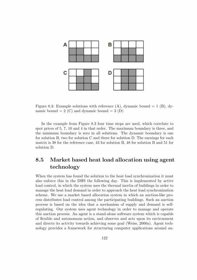
Figure 8.3: Example solutions with reference (A), dynamic bound = 1 (B), dy-namic bound = 2 (C) and dynamic bound = 3 (D)

In the example from Figure 8.3 four time steps are used, which correlate tospot prices of 5, 7, 10 and 4 in that order. The maximum boundary is three, andthe minimum boundary is zero in all solutions. The dynamic boundary is onefor solution B, two for solution C and three for solution D. The earnings for eachmatrix is 38 for the reference case, 43 for solution B, 48 for solution B and 51 forsolution D.

8.5 Market based heat load allocation using agenttechnology

When the system has found the solution to the heat load synchronization it mustalso enforce this in the DHS the following day. This is implemented by activeload control, in which the system uses the thermal inertia of buildings in order tomanage the heat load demand in order to approach the heat load synchronizationscheme. We use a market based allocation system in which an auction-like pro-cess distributes load control among the participating buildings. Such an auctionprocess is based on the idea that a mechanism of supply and demand is self-regulating. Our system uses agent technology in order to manage and operatethis auction process. An agent is a stand-alone software system which is capableof flexible and autonomous action, and observes and acts upon its environmentand directs its activity towards achieving some goal (Weiss, 2000a). Agent tech-nology provides a framework for structuring computer applications around au-

122

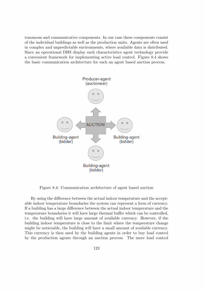
tonomous and communicative components. In our case these components consistof the individual buildings as well as the production units. Agents are often usedin complex and unpredictable environments, where available data is distributed.Since an operational DHS display such characteristics agent technology providea convenient framework for implementing active load control. Figure 8.4 showsthe basic communication architecture for such an agent based auction process.

Figure 8.4: Communication architecture of agent based auction

By using the difference between the actual indoor temperature and the accept-able indoor temperature boundaries the system can represent a form of currency.If a building has a large difference between the actual indoor temperature and thetemperature boundaries it will have large thermal buffer which can be controlled,i.e. the building will have large amount of available currency. However, if thebuilding indoor temperature is close to the limit where the temperature changemight be noticeable, the building will have a small amount of available currency.This currency is then used by the building agents in order to buy load controlby the production agents through an auction process. The more load control

123

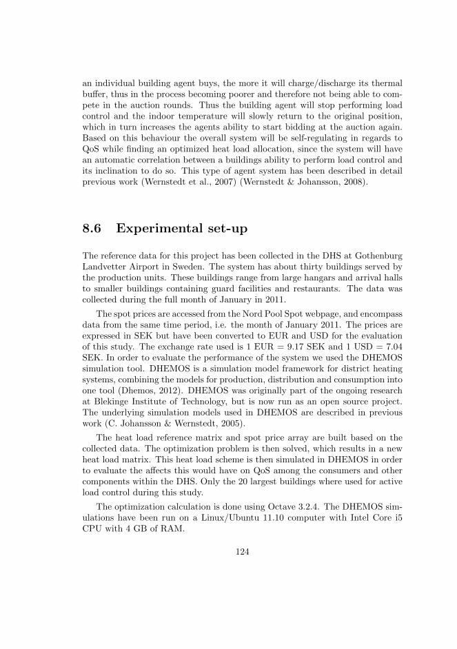
an individual building agent buys, the more it will charge/discharge its thermalbuffer, thus in the process becoming poorer and therefore not being able to com-pete in the auction rounds. Thus the building agent will stop performing loadcontrol and the indoor temperature will slowly return to the original position,which in turn increases the agents ability to start bidding at the auction again.Based on this behaviour the overall system will be self-regulating in regards toQoS while finding an optimized heat load allocation, since the system will havean automatic correlation between a buildings ability to perform load control andits inclination to do so. This type of agent system has been described in detailprevious work (Wernstedt et al., 2007) (Wernstedt & Johansson, 2008).

8.6 Experimental set-up

The reference data for this project has been collected in the DHS at GothenburgLandvetter Airport in Sweden. The system has about thirty buildings served bythe production units. These buildings range from large hangars and arrival hallsto smaller buildings containing guard facilities and restaurants. The data wascollected during the full month of January in 2011.

The spot prices are accessed from the Nord Pool Spot webpage, and encompassdata from the same time period, i.e. the month of January 2011. The prices areexpressed in SEK but have been converted to EUR and USD for the evaluationof this study. The exchange rate used is 1 EUR = 9.17 SEK and 1 USD = 7.04SEK. In order to evaluate the performance of the system we used the DHEMOSsimulation tool. DHEMOS is a simulation model framework for district heatingsystems, combining the models for production, distribution and consumption intoone tool (Dhemos, 2012). DHEMOS was originally part of the ongoing researchat Blekinge Institute of Technology, but is now run as an open source project.The underlying simulation models used in DHEMOS are described in previouswork (C. Johansson & Wernstedt, 2005).

The heat load reference matrix and spot price array are built based on thecollected data. The optimization problem is then solved, which results in a newheat load matrix. This heat load scheme is then simulated in DHEMOS in orderto evaluate the affects this would have on QoS among the consumers and othercomponents within the DHS. Only the 20 largest buildings where used for activeload control during this study.

The optimization calculation is done using Octave 3.2.4. The DHEMOS sim-ulations have been run on a Linux/Ubuntu 11.10 computer with Intel Core i5CPU with 4 GB of RAM.

124

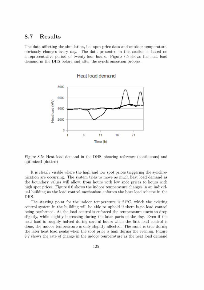
8.7 Results

The data affecting the simulation, i.e. spot price data and outdoor temperature,obviously changes every day. The data presented in this section is based ona representative period of twenty-four hours. Figure 8.5 shows the heat loaddemand in the DHS before and after the synchronization process.

Figure 8.5: Heat load demand in the DHS, showing reference (continuous) andoptimized (dotted)

It is clearly visible where the high and low spot prices triggering the synchro-nization are occurring. The system tries to move as much heat load demand asthe boundary values will allow, from hours with low spot prices to hours withhigh spot prices. Figure 8.6 shows the indoor temperature changes in an individ-ual building as the load control mechanism enforces the heat load scheme in theDHS.

The starting point for the indoor temperature is 21◦C, which the existingcontrol system in the building will be able to uphold if there is no load controlbeing performed. As the load control is enforced the temperature starts to dropslightly, while slightly increasing during the later parts of the day. Even if theheat load is roughly halved during several hours when the first load control isdone, the indoor temperature is only slightly affected. The same is true duringthe later heat load peaks when the spot price is high during the evening. Figure8.7 shows the rate of change in the indoor temperature as the heat load demand

125

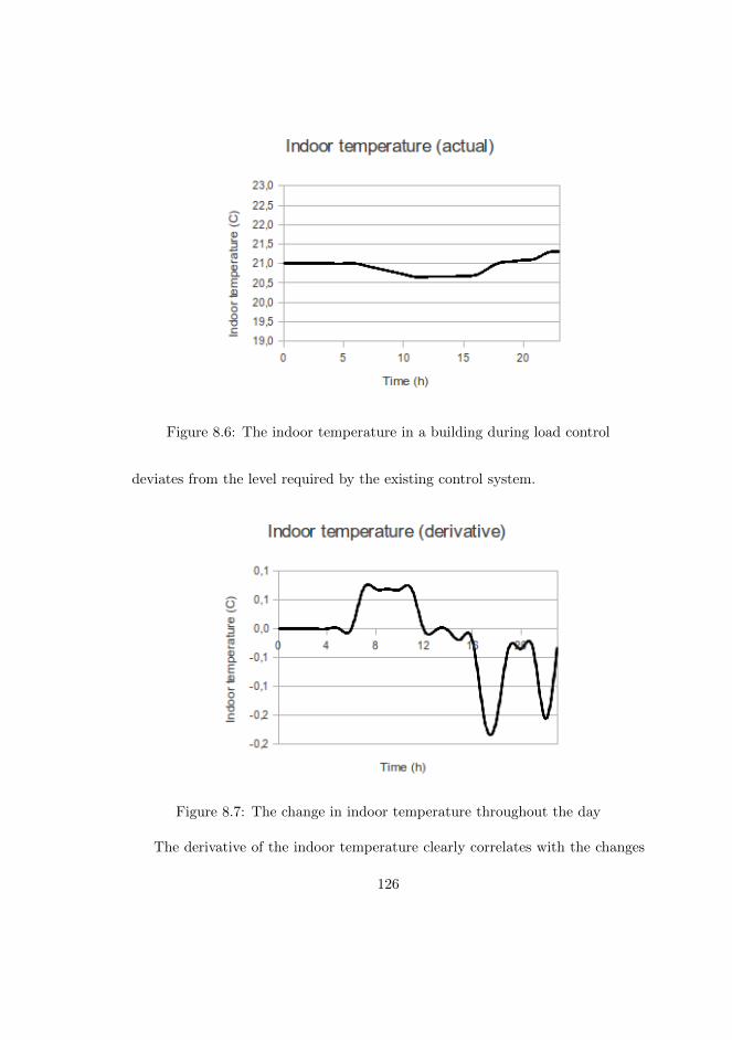
Figure 8.6: The indoor temperature in a building during load control

deviates from the level required by the existing control system.

Figure 8.7: The change in indoor temperature throughout the day

The derivative of the indoor temperature clearly correlates with the changes

126

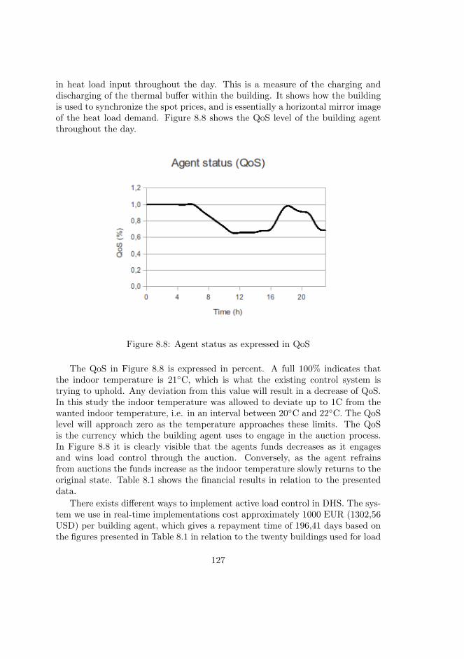
in heat load input throughout the day. This is a measure of the charging anddischarging of the thermal buffer within the building. It shows how the buildingis used to synchronize the spot prices, and is essentially a horizontal mirror imageof the heat load demand. Figure 8.8 shows the QoS level of the building agentthroughout the day.

Figure 8.8: Agent status as expressed in QoS

The QoS in Figure 8.8 is expressed in percent. A full 100% indicates thatthe indoor temperature is 21◦C, which is what the existing control system istrying to uphold. Any deviation from this value will result in a decrease of QoS.In this study the indoor temperature was allowed to deviate up to 1C from thewanted indoor temperature, i.e. in an interval between 20◦C and 22◦C. The QoSlevel will approach zero as the temperature approaches these limits. The QoSis the currency which the building agent uses to engage in the auction process.In Figure 8.8 it is clearly visible that the agents funds decreases as it engagesand wins load control through the auction. Conversely, as the agent refrainsfrom auctions the funds increase as the indoor temperature slowly returns to theoriginal state. Table 8.1 shows the financial results in relation to the presenteddata.

There exists different ways to implement active load control in DHS. The sys-tem we use in real-time implementations cost approximately 1000 EUR (1302,56USD) per building agent, which gives a repayment time of 196,41 days based onthe figures presented in Table 8.1 in relation to the twenty buildings used for load

127

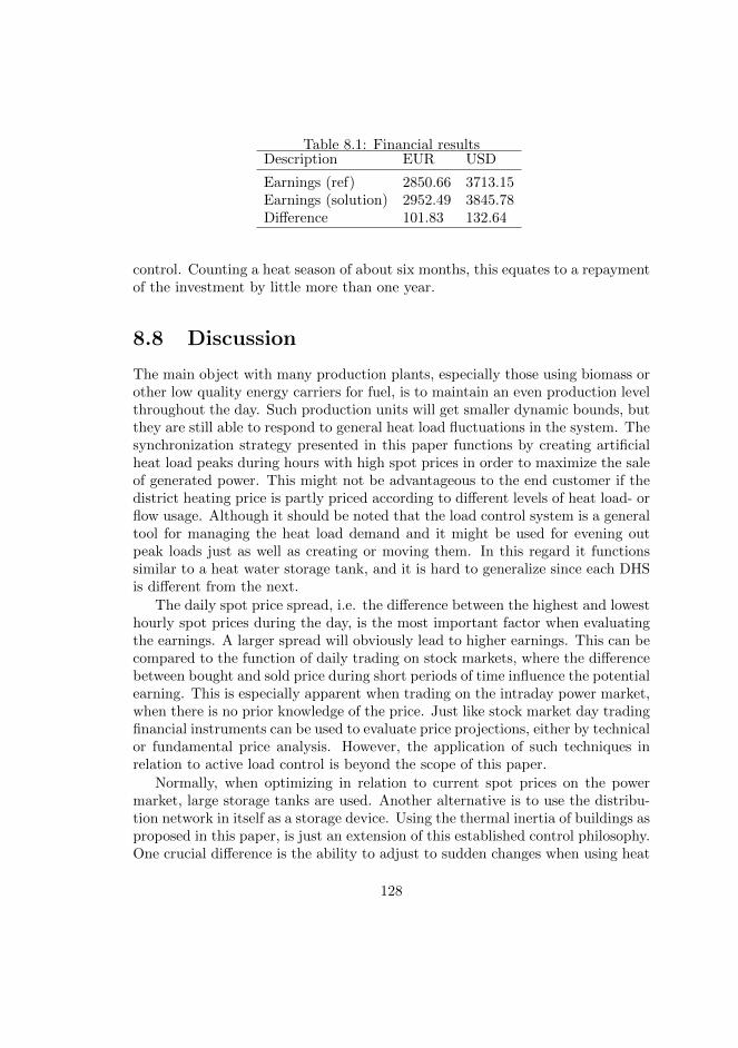
Table 8.1: Financial resultsDescription EUR USD

Earnings (ref) 2850.66 3713.15Earnings (solution) 2952.49 3845.78Difference 101.83 132.64

control. Counting a heat season of about six months, this equates to a repaymentof the investment by little more than one year.

8.8 Discussion

The main object with many production plants, especially those using biomass orother low quality energy carriers for fuel, is to maintain an even production levelthroughout the day. Such production units will get smaller dynamic bounds, butthey are still able to respond to general heat load fluctuations in the system. Thesynchronization strategy presented in this paper functions by creating artificialheat load peaks during hours with high spot prices in order to maximize the saleof generated power. This might not be advantageous to the end customer if thedistrict heating price is partly priced according to different levels of heat load- orflow usage. Although it should be noted that the load control system is a generaltool for managing the heat load demand and it might be used for evening outpeak loads just as well as creating or moving them. In this regard it functionssimilar to a heat water storage tank, and it is hard to generalize since each DHSis different from the next.

The daily spot price spread, i.e. the difference between the highest and lowesthourly spot prices during the day, is the most important factor when evaluatingthe earnings. A larger spread will obviously lead to higher earnings. This can becompared to the function of daily trading on stock markets, where the differencebetween bought and sold price during short periods of time influence the potentialearning. This is especially apparent when trading on the intraday power market,when there is no prior knowledge of the price. Just like stock market day tradingfinancial instruments can be used to evaluate price projections, either by technicalor fundamental price analysis. However, the application of such techniques inrelation to active load control is beyond the scope of this paper.

Normally, when optimizing in relation to current spot prices on the powermarket, large storage tanks are used. Another alternative is to use the distribu-tion network in itself as a storage device. Using the thermal inertia of buildings asproposed in this paper, is just an extension of this established control philosophy.One crucial difference is the ability to adjust to sudden changes when using heat

128

load demand in buildings. Load control in a building can react as quickly as thevalves on the heat exchanger can move, while a storage tank requires much longerpre-heating and charging strategies. In practice this is like comparing secondsto hours. This is especially important in relation to intraday power markets, inwhich the energy company has no prior knowledge of the electricity price. Thefinancial gain in such markets is also potentially larger since they tend to be morevolatile and thus resulting in larger spreads.

There is also another, quite important, difference between using the thermalbuffer of buildings instead of storage tanks, and this is the installation and main-tenance costs involved. The price for a storage tank is heavily dependent on thecurrent price of steel. The total installation cost is more or less linear with thesteel price for storage tanks up to about 50 MW, after which it increases evenmore since the added physical constraints of such large tanks require increased di-mensions. A storage tank with a heat load of about 50 MW costs about 3 millionEUR (3,9 million USD) while a corresponding system using active load controlwill cost approximately 1 million EUR (1,3 million USD). The maintenance costis also substantially lower.

Another solution for spot price optimization is to increase the pressure headthroughout the DHS, which enables the possibility of lower return temperaturesin the primary flow network. Since this result in a higher temperature gradient inthe production turbine, it is possible to get a higher output from the power gen-eration. However, having excessively high pressure heads is expensive, and mightalso introduce other problems in relation to component behaviour. Performingload control, on the other hand, helps lower the primary return temperaturewithout requiring higher pressure heads (Wernstedt, Johansson, & Wollerstrand,2008). By coordinating this behaviour among a larger group of buildings it ispossible to achieve a lowered temperature on average also.

During this study we have used simulation to evaluate the behaviour of theload control system. However, the products used to implement such systems existon the market today, and have been extensively evaluated in previous work. Thismakes it possible for us to draw conclusions about the system limits in regards tothe operational managing of heat load demand, which enables us to set realisticboundaries for the synchronization problem.

A basic problem with solutions such as the one proposed in this paper, isthat if all parties active on the market used them it would obviously affect theoutcome of the trading. In practice this is not a problem, since CHP represents avery small part of all power being traded on the open markets. In Sweden morethan eighty percent of all power is produced by hydro power or nuclear power,while wind power, CHP and other marginal production types make up for therest.

129

8.9 Conclusions

In this paper we have presented a model for finding an optimized synchronizationbetween heat load demand and spot prices when using CHP. This is then imple-mented through active load control by using the thermal inertia within individualbuildings. The model takes into account the specific boundary conditions presentfor individual production unit configurations in relation to operational limits ofload control in individual buildings. This is done by using a market based auctionprocess as a mediating interface between the buildings and the production units.Agent technology is used in order to implement this auction process. Each build-ing is assigned an individual agent, which will try to maximize the load controlwhile maintaining a sufficient level of QoS.

The results show clear financial incentives for implementing this type of tech-nology, having a repayment time of less than two heating seasons. At the sametime it is concluded that it is possible to achieve this without jeopardizing theQoS among the participating buildings.

The financial benefits of this technology are dependent on the spread of thespot prices, in relation to the boundary conditions in the system. But since thisspread is normally quite large, even systems with tight dynamic boundaries willexperience improved earnings.

8.10 Future work

Based on the flexibility of the agent based load control solution it is likely that thetype of solution presented in this paper is appropriate for managing synchroniza-tion in relation to intraday power markets. Since the spot prices are not knownin advance it places even more focus on high flexibility and the ability to quicklyadjust the power production. A distinguishing factor of such intraday marketsis their tendency to be very volatile with highly fluctuating prices, much moreso than the normal day-ahead power markets. However, such an environmentdoes place additional demands on the ability to evaluate projections of heat loaddemand as well as spot prices. Hence, further investigation and incorporation ofsuch techniques in the present model should be a primary goal in the near future.

Another interesting venue is to further develop the optimization model inorder to use dynamical sizing of the heat blocks. This would enable a closercorrelation with individual consumers or groups of consumers, and would makepossible a direct mathematical derivation between the entity instigating loadcontrol (i.e. the energy company) and the entity performing the load control(i.e. the building). It would also enable a route for quantifying the contributionof individual buildings when performing load control, in turn enabling a way tocompensate building owners for letting the energy company use their resources.

130

8.11 Acknowledgement

We would like to thank Swedavia for letting us use operational data from thedistrict heating system at Gothenburg Landvetter Airport.

Also we would like to thank the DHEMOS team for support when developingand adapting the simulation models used by DHEMOS.

Lastly we would like to thank NODA Intelligent Systems AB for supportregarding server and data access during this project.

131

132

Chapter 9

Paper VIII - Smart heatgrid on an intraday powermarket

District heating systems (DHS) is in many countries an important part of theheating infrastructure, especially in and around urban areas. Combined heat andpower (CHP) production makes it possible to producer heat while simultaneouslyproducing power. This combination help maximize the energy efficiency in pro-duction, often reaching an 80-90% utilization level of the primary fuel, comparedto around 30-50% in a traditional power plant. The heat produced in the CHPplant is used to heat the adjacent DHS, while the power is transferred and soldon the power market. The work presented in this paper relates to the Nord PoolSpot power market, which is the leading power market in Europe and one of thelargest in the world. On Nord Pool Spot power is bought and sold based on hourlyspot prices, facilitated by the primary day-ahead market and the supplementarybalancing intraday market.

Since it isnt possible to separate the physical process of producing heat andpower in a CHP production facility, the energy company will want to synchronizehigh heat load production with high spot prices for power whenever possible. Thiscan be done by using large storage tanks where heat is buffered during hourswith high spot prices, while then distributed to the DHS as the heat load demandincreases. However, such storage tanks are expensive to build and maintain,and they have limited operational dynamics. An alternative is to use the actualbuildings connected to the DHS, in order to utilize their thermal inertia by theuse of active load control.

133

This paper presents a multi-agent system (MAS) designed to bridge the in-formation gap between energy companies and building owners in order to enablethe use of system-wide active load control in order to synchronization heat loadand spot prices. The presented scheme provides a self-regulating market analogyin which agents act to allocate load control resources. Each participating build-ing is assigned a consumer agent, while each production unit is represented by aproduction agent. These agents interact on the market analogy which is in turnsupervised by a market agent. The work in this paper is focused on the intra-day market although the underpinning synchronization scheme is suitable for theday-ahead market as well as the intraday market. The results show considerablegains for participating entities when applying the presented strategy to the oftenvolatile intraday spot price market.

9.1 Introduction

This work concerns the ability to use active load control in district heating sys-tems (DHS) in order to maximize revenue from the power market when usingcombined heat and power generation. A district heating system consists of oneor more production plants connected to a distribution pipe network which in turnis connected to heat exchanger substations at consumer buildings. Normally wa-ter is used as the energy transfer medium within the pipes, although some oldersystems use steam. Production units can use more or less any available boilertypes, as long as they are able to heat the water or steam to sufficient levels.This makes it possible to use a wide range of primary fuels such as coal, oil,biogas or nuclear power and even makes it possible to utilize low or mediumgrade energy carriers such as peat, different types of biomass or waste heat fromnearby industries. District heating is the predominant heating type in urban ar-eas in northern and eastern parts of Europe including Russia and former Sovietcountries, although the technology is present all around the world and gainingincreased acceptance throughout North America and Asia (Constinescu, 2007).

A combined heat and power (CHP) plant produces electrical power as wellas heat for the DHS. In a CHP plant water is boiled to steam which is in turnoverheated to about 500-600 C. The steam is then used to run a turbine, whichin turn is connected to a generator which converts the mechanical energy toelectrical energy. When the steam has passed through the turbine its pressureand temperature is decreased in a condenser unit which absorbs the heat fromthe steam and transfers it to the water medium in the district heating system.The condensed water (previously steam) is then led back to the original boilerin which the process is repeated. In a normal power plant the heat is normallyemitted as waste heat in the turbine/generator process. By instead utilizingthis heat a CHP plant is capable of achieving higher levels of energy efficiency

134

in relation to the primary fuel (80-90%) than traditional power plants (30-50%)(Horlock, 2008). CHP plants are common in many DHS and when building newproduction plants CHP is many times the preferred choice of production, since itsefficient use of primary energy makes the system financially and environmentallysound.

The power produced in a CHP plant is normally sold on a regional, nationalor international power market. The work described in this paper is related tothe Nord Pool Spot power market which covers large parts of Northern Europeand which is one of the largest power markets in the world. However, the basicpremises are similar for most de-regulated power markets, in that the prices areset based on a balance between supply and demand.

The Nord Pool Spot market is divided into two separate market parts, namelythe day-ahead market (Elspot) and the intraday market (Elbas) (NordPoolSpot,2012). The larger of the two is the day-ahead market through which the majorityof all power is being bought and sold. Here power contracts are made for deliverythe following day. The contracts cover hourly spot prices throughout the nextday, and are published on the afternoon the day before. In addition to this thereis also an intraday market which supplements the day-ahead market by securingthe balance between supply and demand. Traditionally the intraday market hasbeen used as a balancing market mechanism in order to bridge specific incidentssuch as unplanned operational stops in nuclear power plants. However, as morewind power production enters the grid, the need for intraday balancing increases.Wind power is undeniably a sustainable and environmentally desirable productiontype, but it is also somewhat unpredictable. A growing percentage of sustainablepower production will thus only increase the importance of the intraday powermarket. The very nature of the intraday market makes for a higher volatilityin price compared to the day-ahead market. It is this characteristic that makesthe intraday market enticing for power market actors which have the ability todynamically adapt and conform to that same volatility.

Load control is the ability to actively control the heat load in a DHS. Thisability is what makes it possible for DHS operator to adapt to the changing con-ditions on an intraday market by dynamically rearranging the heat load demandamong the consumer stations. A similar tool, albeit less flexible, is the use ofstorage tanks which can be charged and discharged according to changes in spotprice instead of directly feeding the heat into the DHS. However, consideringtheir limited operational dynamics, the use of storage tank based strategies ismore suited for the day-ahead power market (Andrepont, 2012). Load control inDHS can be implemented either actively or passively. Passive load control triesto influence the consumers to act in certain ways, through the use of indirectmethods such as differentiating heat load- or flow rates. Such methods are notguaranteed to work, i.e. a consumer might willingly choose to ignore to adapt

135

to current flow rates, or more likely, will not have the technical ability to doanything much the rate even if they wanted. Such methods are also much tooinflexible for applications considered in relation to the dynamics of an intradaymarket. Active load control, on the other hand, provides a technical frameworkfor performing instant heat load manipulation among the consumers.

Previous work has presented the basic centralized synchronization strategyfor heat load and spot price management in relation to a basic day-ahead powermarket (C. Johansson, Wernstedt, & Davidsson, 2012a). The work described inthis paper follows on that previous work by expanding the problem domain to en-compass the entire energy system from a multi-agent system (MAS) perspective.Also, the more volatile, and thus potentially more profitable, intraday marketis considered. In addition to this the MAS approach provides a framework forcompensating the active consumer systems in relation to their actual level ofparticipation. The system is evaluated through simulation experimentation.

9.2 Related work

Different strategies for using heat storage in order to improve operations are pre-sented in (Wigbels, Bohm, & Sipilae, 2005) and (Rolfsman, 2003). The potentialof using building mass as short term heat storage is quantified and described in(Olsson Ingvarsson & Werner, 2008). Further work on thermal mass in buildingsis presented in (Hietmaki et al., 2003). All these works show consistently thatsubstantial amounts of energy can be charged and discharged within the structureof individual buildings. In other words, due to the thermal inertia of buildings itis possible to manipulate the heat load demand of a building without affecting theindoor climate (Concrete for Energy Efficient Buildings The benefits of thermalmass, 2007).

Active load control for individual buildings has been studied since at leastthe early eighties, although the technical constraints of the hardware of thattime limited the practical use of such systems. However, even those early worksrecognized the potential of the basic load control technique (Osterlind, 1982). Theimportance of two-way communication in order to enable feedback throughoutthe system was also early established (Osterlind, 1990).

The theoretical aspects of load control in district heating systems were stud-ied in (Sipila & Karkkainen, 2000), while a real-time industrial load controlsystem was implemented and evaluated in (Wernstedt & Johansson, 2009) and(Wernstedt et al., 2008). Load control in electrical grids through the use of time-varying pricing is studied in (Newsham & Bowker, 2010). It is concluded thatdirect load control, in the sense of technology able to response to the pricingscheme, is imperative in order to attain desirable levels of response.

The heating and cooling behaviour of buildings have been studied in many

136

projects. Pre-cooling and demand limiting is studied extensively in (Xu, Haves,Piette, & Zagreus, 2006) and (Braun, 2003). The studies conclude that it is pos-sible to improve demand responsiveness while maintaining acceptable comfortconditions. Heating control strategies are studied in (Bjorsell, n.d.). More adap-tive learning algorithms for heating systems are presented in (Rogers, Maleki,Ghosh, & Jennings, 2011) and (Chahwane, Stephan, Wurtz, E., & Zuber, 2011).The common denominator of these systems is that they all directly or indirectlymake use of the thermal inertia of buildings in order to streamline the heating orcooling demand in buildings.

As the control strategies become increasingly complex the desire to continu-ously evaluate the resulting thermal behaviour will become more apparent. Thiscan be done either by simulation, sensor readings or by a combination of thetwo. A study of how to model the heat dynamics in a building using stochas-tic differential equations from a simulation perspective is presented in (Andersenet al., 2000). The impact of using real-time sensory equipment is evaluated in(C. Johansson et al., 2010a).

A theoretical MAS platform for load control in district heating systems hasbeen previously described in (Wernstedt et al., 2007). Such a system has sincebeen implemented in a real-time industrial setting which was described in [25].The implemented system confirmed that the system was able to perform contin-uous load control schemes corresponding to substantial amounts of the total heatload. Later experiments with the same type of system have shown even greaterability to perform load control (C. Johansson, 2010).

The heat load in a DHS is mainly dependant on the outdoor temperaturein combination with social behavior affecting tap water and ventilation. Sev-eral studies have been performed in regards to forecasting this behavior. Basicmodels relating to short-term heat load forecasting are presented in (Jonsson,2002) and (Dotzauer, 2002). A seasonal autoregressive integrated moving av-erage (SARIMA) process is presented in (Grosswindhager et al., 2011), whilebasic Box-Jenkins autoregressive integrated moving average (ARIMA) methodsare presented in (Box & G.M., 1991). Further studies of such methods are pre-sented in (Chramcov, Dostal, & Balate, 2009). A grey-box approach explicitlyusing climate measures to forecast heat consumption in a large geographical areais presented in (Nielsen & Madsen, 2006).

9.3 Multi-agent system overview

The general framework for the MAS consists of three different agent types inter-acting in order to achieve the overarching goal of maximizing profits in relationto CHP production while simultaneously ensuring sufficient levels of Quality ofService (QoS) among the participating buildings. The consumer agent is the

137

agent responsible for supervising and controlling the heat load at the individualconsumer sub-stations. The producer agent calculates the need for active loadcontrol based on projections of the heat load demand in relation to current andfuture power spot prices. Finally the market agent is responsible for coordinat-ing and allocating active load control among the consumer agent based on therequirements of the producer agent.

The different agents act according to their individual conditions and con-straints, although they do hold certain knowledge in common throughout theMAS. The same weather forecast is normally shared among all the agents, al-though its perceived effect on the individual agents might differ. Historical dataregarding the allocating process from the market agent is also freely availableamong the agents, as well as historical data regarding power market spot prices.Based on this it is possible for producer agents as well as consumer agents tocalculate their own projections for spot prices and heat load demand, and hencedevise strategies in order to further their individual goals. For a productionagent this basically equates to selecting suitable valuation levels for load controland constructing allocation contracts considering an appropriate margin of er-ror. Likewise, the goal for a consumer agent is to get paid as much as possiblefor performing current load control, while simultaneously maintaining a suitablepreparation level for future load control and ensuring sufficient QoS.

9.3.1 Consumer agent

The consumer agent (CA) is responsible for maintaining an acceptable level ofQoS while at the same time performing load control. These aspects are intercon-nected since a CA uses its internal QoS status as measurement of load controlability, and can thus only perform load control if the current levels of QoS allowit. In the context of this work QoS is related purely to the indoor temperature. Inorder to calculate the indoor temperature the CA uses an energy balance model,which in its most fundamental form is shown in equation 9.1.

∆Tindoor = Hin −Hout (9.1)

where Hin is the total heat load being input into the building and Hout isthe total amount of heat escaping the building. Any in-balance between thesevalues will result in a non-zero ∆Tindoor, i.e. a change in the indoor temperaturewill occur. Such energy balance equations can be modelled arbitrarily complex.However, in order to adapt to limitations in the current hardware a model basedon two temperature zones was developed. The model thus calculates one valuefor the indoor air temperature and one value for the average temperature of theclimate shell of the building. Another issue with such energy balance models is

138

that they tend to require a large amount of well calibrated parameters, especiallyin relation to the Hout part of the equation, which is exactly what is to beavoided in order to keep the model simple enough to use in practical settings inmany buildings. The presented model is built around a traditional heat balancemodel, although it has been adapted to avoid this very problem. This has beenachieved by translating the heat load balance from a physical model into a blackbox simulation model, in which certain parameters do not necessarily have anyrelation to actual physical counterparts. By locking parts of the equation and onlyletting certain parameters be variable it is possible to retain the characteristicsof the original equation (calculating correctly), while simultaneously adding thepreviously lacking characteristics (ease of use). The resulting model is shown inequation 9.2.

4Ti = (1.46 ∗ T2 ∗ (Tb − Ti) + 38.9 ∗ (To − Ti)+

Hin)/(T1 ∗ 1000000)4Tb = (1.46 ∗ T2 ∗ (To − Tb) + 1.46 ∗ T2 ∗ (Ti − Tb)+

(1− Vs) ∗Hin)/45000000

(9.2)

where Ti, Tb and To are the indoor, building structure and outdoor tem-peratures. Hin is the total heat load input into the building and Vs is a statecontrolled adaptive variable used to adjust the behaviour of the model accordingto observations in regards to the recovery of temporary temperature fluctuations.The model is first and foremost designed to be used in relation to fast thermalprocesses; normally the temperature range is only a few degrees up and down andthe simulation time frame at most a few hours. The steady state energy balancemodels which equation 9.2 originates from are generally poorly equipped to han-dle such transient behaviour. Due to constraints in regards to computationallycomplexity the model is not able to explicitly take into account the dynamicallydifferentiating influence of the different modes of heat transfer, i.e. conduction,convection and radiation. Another aspect is the free heat load input from socialbehaviour, electric appliances or from outdoor climate variations, which is nor-mally modelled by adding stochastic variables. This is also not feasible due tothe added complexity involved in such a solution. In order to still get a goodapproximation of the observed behaviour the Vs value was instead added intothe model. The Vs variable can be seen as a catalyst which changes the speed ofreaction within the thermal process. The variable can only take two values, i.e.0 and 1. The state evaluation is performed according to equation 9.3.

f(Tw, Ti, Te) =

{1 if Tw − Ti ≤ Te0 if Tw − Ti > Te

(9.3)

139

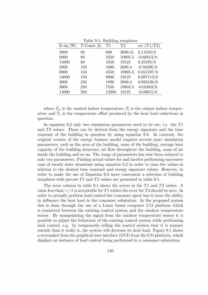
Table 9.1: Building templatesE-sig [W] T-Const [h] T1 T2 err (T1/T2)

2000 80 600 2686.41 0.11342/08000 80 2250 10905.5 -0.86813/014000 80 4350 19125 0.35476/02000 150 1080 2686.4 -0.50236/08000 150 4550 10905.5 0.051597/014000 150 8000 19125 0.097113/02000 250 1890 2686.4 0.056136/08000 250 7550 10905.5 -0.01603/014000 250 13200 19125 -0.03615/0

where Tw is the wanted indoor temperature, Ti is the output indoor temper-ature and Te is the temperature offset produced by the heat load reductions inquestion.

In equation 9.2 only two simulation parameters need to be set, i.e. the T1and T2 values. These can be derived from the energy signature and the timeconstant of the building in question by using equation 9.2. In contrast, theoriginal version of the energy balance model requires several more simulationparameters, such as the area of the building, mass of the building, average heatcapacity of the building structure, air flow throughout the building, mass of airinside the building and so on. The range of parameters has now been reduced toonly two parameters. Finding actual values for and involve performing successiveruns of steady state situations using equation 9.2 in order to tune the values inrelation to the desired time constant and energy signature values. However, inorder to make the use of Equation 9.2 more convenient a selection of buildingtemplates with pre-set T1 and T2 values are presented in table 9.1.

The error column in table 9.1 shows the errors in the T1 and T2 values. Avalue less than +/-1 is acceptable for T1 whiles the error for T2 should be zero. Inorder to actually perform load control the consumer agent has to have the abilityto influence the heat load in the consumer substation. In the proposed systemthis is done through the use of a Linux based computer I/O platform whichis connected between the existing control system and the outdoor temperaturesensor. By manipulating the signal from the outdoor temperature sensor it ispossible to adjust the behaviour of the existing control system while performingload control, e.g. by temporarily telling the control system that it is warmeroutside than it really is, the system will decrease its heat load. Figure 9.1 showsa screenshot from the graphical user interface (GUI) from the I/O platform, whichdisplays an instance of load control being performed in a consumer substation.

140

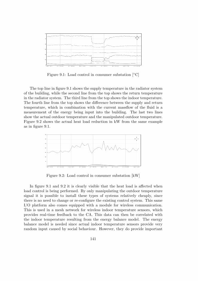
Figure 9.1: Load control in consumer substation [◦C]

The top line in figure 9.1 shows the supply temperature in the radiator systemof the building, while the second line from the top shows the return temperaturein the radiator system. The third line from the top shows the indoor temperature.The fourth line from the top shows the difference between the supply and returntemperature, which in combination with the current massflow of the fluid is ameasurement of the energy being input into the building. The last two linesshow the actual outdoor temperature and the manipulated outdoor temperature.Figure 9.2 shows the actual heat load reduction in kW from the same exampleas in figure 9.1.

Figure 9.2: Load control in consumer substation [kW]

In figure 9.1 and 9.2 it is clearly visible that the heat load is affected whenload control is being performed. By only manipulating the outdoor temperaturesignal it is possible to install these types of systems relatively cheaply, sincethere is no need to change or re-configure the existing control system. This sameI/O platform also comes equipped with a module for wireless communication.This is used in a mesh network for wireless indoor temperature sensors, whichprovides real-time feedback to the CA. This data can then be correlated withthe indoor temperature resulting from the energy balance model. The energybalance model is needed since actual indoor temperature sensors provide veryrandom input caused by social behaviour. However, they do provide important

141

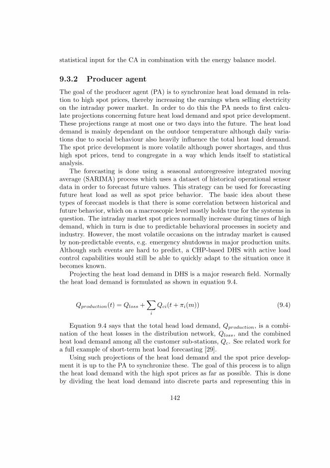
statistical input for the CA in combination with the energy balance model.

9.3.2 Producer agent

The goal of the producer agent (PA) is to synchronize heat load demand in rela-tion to high spot prices, thereby increasing the earnings when selling electricityon the intraday power market. In order to do this the PA needs to first calcu-late projections concerning future heat load demand and spot price development.These projections range at most one or two days into the future. The heat loaddemand is mainly dependant on the outdoor temperature although daily varia-tions due to social behaviour also heavily influence the total heat load demand.The spot price development is more volatile although power shortages, and thushigh spot prices, tend to congregate in a way which lends itself to statisticalanalysis.

The forecasting is done using a seasonal autoregressive integrated movingaverage (SARIMA) process which uses a dataset of historical operational sensordata in order to forecast future values. This strategy can be used for forecastingfuture heat load as well as spot price behavior. The basic idea about thesetypes of forecast models is that there is some correlation between historical andfuture behavior, which on a macroscopic level mostly holds true for the systems inquestion. The intraday market spot prices normally increase during times of highdemand, which in turn is due to predictable behavioral processes in society andindustry. However, the most volatile occasions on the intraday market is causedby non-predictable events, e.g. emergency shutdowns in major production units.Although such events are hard to predict, a CHP-based DHS with active loadcontrol capabilities would still be able to quickly adapt to the situation once itbecomes known.

Projecting the heat load demand in DHS is a major research field. Normallythe heat load demand is formulated as shown in equation 9.4.

Qproduction(t) = Qloss +∑i

Qci(t+ πi(m)) (9.4)

Equation 9.4 says that the total head load demand, Qproduction, is a combi-nation of the heat losses in the distribution network, Qloss, and the combinedheat load demand among all the customer sub-stations, Qc. See related work fora full example of short-term heat load forecasting [29].

Using such projections of the heat load demand and the spot price develop-ment it is up to the PA to synchronize these. The goal of this process is to alignthe heat load demand with the high spot prices as far as possible. This is doneby dividing the heat load demand into discrete parts and representing this in

142

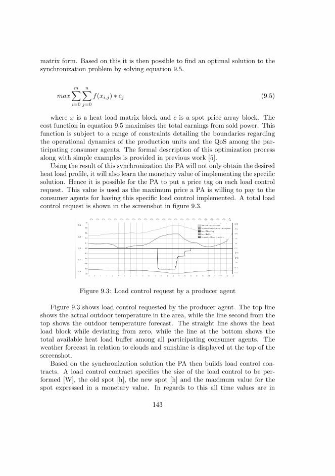
matrix form. Based on this it is then possible to find an optimal solution to thesynchronization problem by solving equation 9.5.

max

m∑i=0

n∑j=0

f(xi,j) ∗ cj (9.5)

where x is a heat load matrix block and c is a spot price array block. Thecost function in equation 9.5 maximises the total earnings from sold power. Thisfunction is subject to a range of constraints detailing the boundaries regardingthe operational dynamics of the production units and the QoS among the par-ticipating consumer agents. The formal description of this optimization processalong with simple examples is provided in previous work [5].

Using the result of this synchronization the PA will not only obtain the desiredheat load profile, it will also learn the monetary value of implementing the specificsolution. Hence it is possible for the PA to put a price tag on each load controlrequest. This value is used as the maximum price a PA is willing to pay to theconsumer agents for having this specific load control implemented. A total loadcontrol request is shown in the screenshot in figure 9.3.

Figure 9.3: Load control request by a producer agent

Figure 9.3 shows load control requested by the producer agent. The top lineshows the actual outdoor temperature in the area, while the line second from thetop shows the outdoor temperature forecast. The straight line shows the heatload block while deviating from zero, while the line at the bottom shows thetotal available heat load buffer among all participating consumer agents. Theweather forecast in relation to clouds and sunshine is displayed at the top of thescreenshot.

Based on the synchronization solution the PA then builds load control con-tracts. A load control contract specifies the size of the load control to be per-formed [W], the old spot [h], the new spot [h] and the maximum value for thespot expressed in a monetary value. In regards to this all time values are in

143

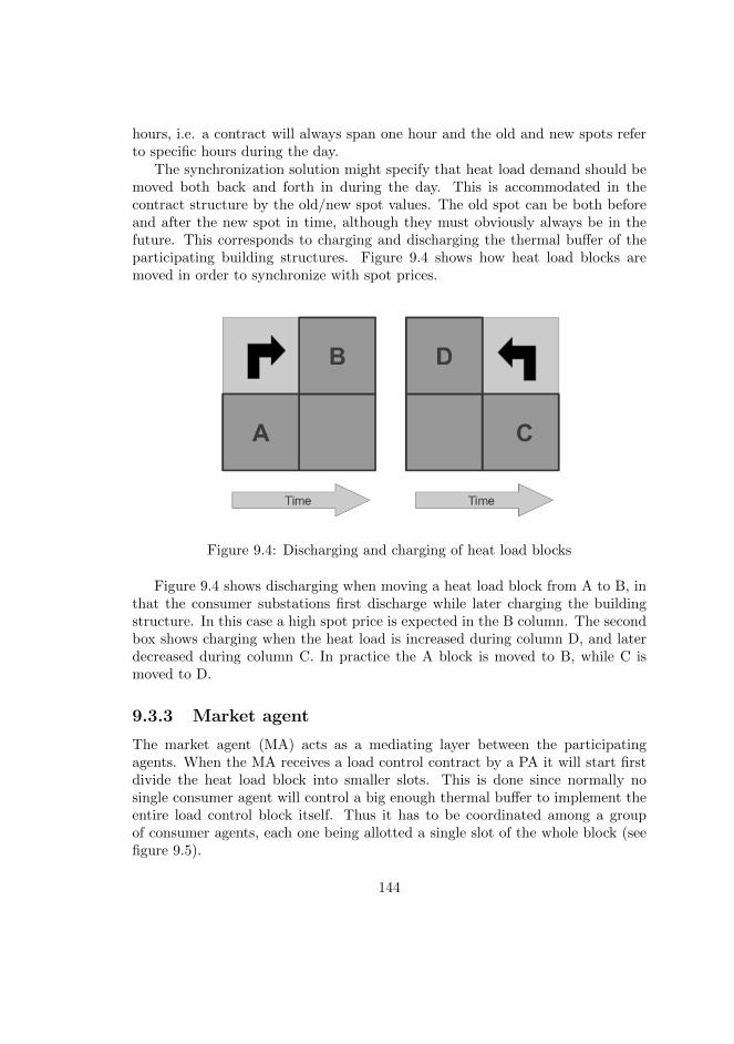
hours, i.e. a contract will always span one hour and the old and new spots referto specific hours during the day.

The synchronization solution might specify that heat load demand should bemoved both back and forth in during the day. This is accommodated in thecontract structure by the old/new spot values. The old spot can be both beforeand after the new spot in time, although they must obviously always be in thefuture. This corresponds to charging and discharging the thermal buffer of theparticipating building structures. Figure 9.4 shows how heat load blocks aremoved in order to synchronize with spot prices.

Figure 9.4: Discharging and charging of heat load blocks

Figure 9.4 shows discharging when moving a heat load block from A to B, inthat the consumer substations first discharge while later charging the buildingstructure. In this case a high spot price is expected in the B column. The secondbox shows charging when the heat load is increased during column D, and laterdecreased during column C. In practice the A block is moved to B, while C ismoved to D.

9.3.3 Market agent

The market agent (MA) acts as a mediating layer between the participatingagents. When the MA receives a load control contract by a PA it will start firstdivide the heat load block into smaller slots. This is done since normally nosingle consumer agent will control a big enough thermal buffer to implement theentire load control block itself. Thus it has to be coordinated among a groupof consumer agents, each one being allotted a single slot of the whole block (seefigure 9.5).

144

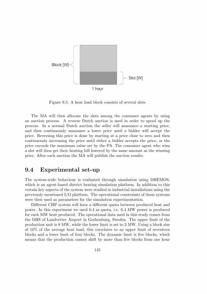
Figure 9.5: A heat load block consists of several slots

The MA will then allocate the slots among the consumer agents by usingan auction process. A reverse Dutch auction is used in order to speed up theprocess. In a normal Dutch auction the seller will announce a starting price,and then continuously announce a lower price until a bidder will accept theprice. Reversing this price is done by starting at a price close to zero and thencontinuously increasing the price until either a bidder accepts the price, or theprice exceeds the maximum value set by the PA. The consumer agent who winsa slot will then get their heating bill lowered by the same amount as the winningprice. After each auction the MA will publish the auction results.

9.4 Experimental set-up

The system-wide behaviour is evaluated through simulation using DHEMOS,which is an agent-based district heating simulation platform. In addition to thiscertain key aspects of the system were studied in industrial installations using thepreviously mentioned I/O platform. The operational constraints of these systemswere then used as parameters for the simulation experimentation.

Different CHP system will have a different quota between produced heat andpower. In this experiment we used 0.4 as quota, i.e. 0.4 MW power is producedfor each MW heat produced. The operational data used in this study comes fromthe DHS of Landvetter Airport in Gothenburg, Sweden. The upper limit of theproduction unit is 8 MW, while the lower limit is set to 2 MW. Using a block sizeof 10% of the average heat load, this correlates to an upper limit of seventeenblocks and a lower limit of four blocks. The dynamic limit is five blocks, whichmeans that the production cannot shift by more than five blocks from one hour

145

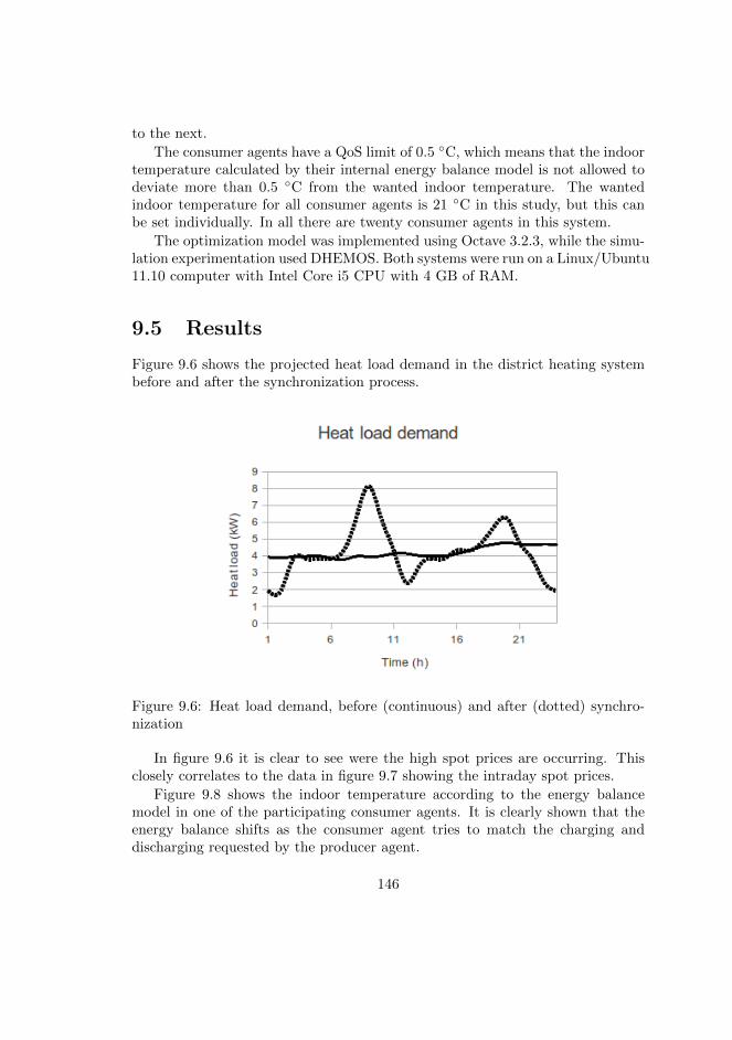
to the next.

The consumer agents have a QoS limit of 0.5 ◦C, which means that the indoortemperature calculated by their internal energy balance model is not allowed todeviate more than 0.5 ◦C from the wanted indoor temperature. The wantedindoor temperature for all consumer agents is 21 ◦C in this study, but this canbe set individually. In all there are twenty consumer agents in this system.

The optimization model was implemented using Octave 3.2.3, while the simu-lation experimentation used DHEMOS. Both systems were run on a Linux/Ubuntu11.10 computer with Intel Core i5 CPU with 4 GB of RAM.

9.5 Results

Figure 9.6 shows the projected heat load demand in the district heating systembefore and after the synchronization process.

Figure 9.6: Heat load demand, before (continuous) and after (dotted) synchro-nization

In figure 9.6 it is clear to see were the high spot prices are occurring. Thisclosely correlates to the data in figure 9.7 showing the intraday spot prices.

Figure 9.8 shows the indoor temperature according to the energy balancemodel in one of the participating consumer agents. It is clearly shown that theenergy balance shifts as the consumer agent tries to match the charging anddischarging requested by the producer agent.

146

Figure 9.7: Hourly spot prices on the intraday market

Figure 9.8: Indoor temperature according to energy balance model

147

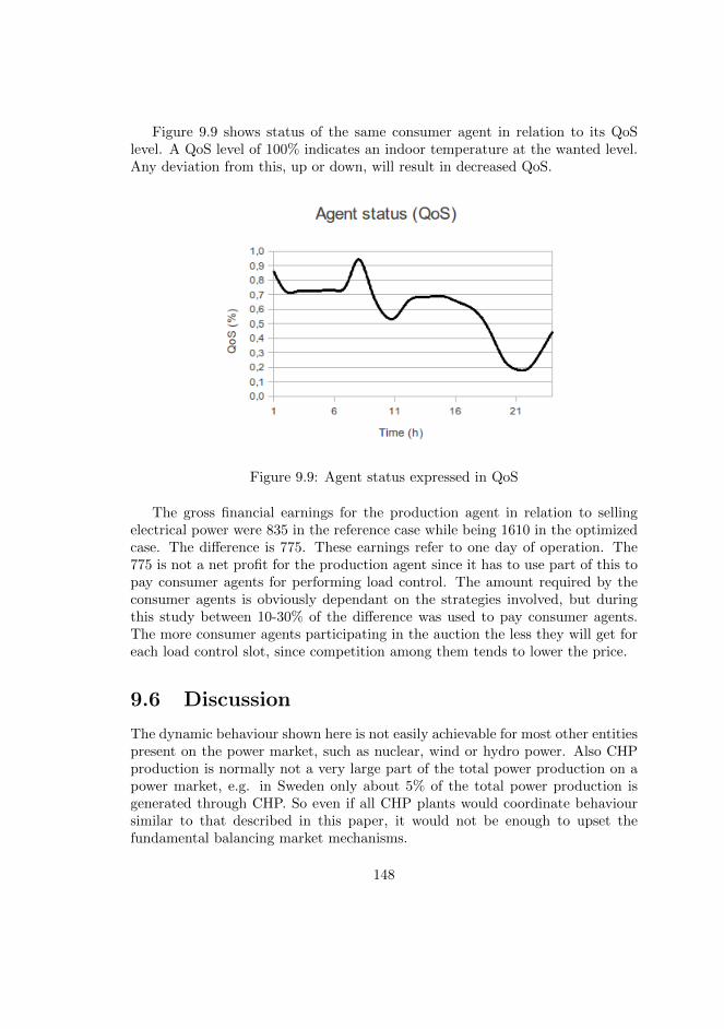
Figure 9.9 shows status of the same consumer agent in relation to its QoSlevel. A QoS level of 100% indicates an indoor temperature at the wanted level.Any deviation from this, up or down, will result in decreased QoS.

Figure 9.9: Agent status expressed in QoS

The gross financial earnings for the production agent in relation to sellingelectrical power were 835 in the reference case while being 1610 in the optimizedcase. The difference is 775. These earnings refer to one day of operation. The775 is not a net profit for the production agent since it has to use part of this topay consumer agents for performing load control. The amount required by theconsumer agents is obviously dependant on the strategies involved, but duringthis study between 10-30% of the difference was used to pay consumer agents.The more consumer agents participating in the auction the less they will get foreach load control slot, since competition among them tends to lower the price.

9.6 Discussion

The dynamic behaviour shown here is not easily achievable for most other entitiespresent on the power market, such as nuclear, wind or hydro power. Also CHPproduction is normally not a very large part of the total power production on apower market, e.g. in Sweden only about 5% of the total power production isgenerated through CHP. So even if all CHP plants would coordinate behavioursimilar to that described in this paper, it would not be enough to upset thefundamental balancing market mechanisms.

148

Even using a synchronization scheme such as the one proposed in this paper, itwould probably not be preferable to commit all power production to the intradaymarket, since there is a chance that the market will be balanced due to theday-ahead market. Therefore a strategy which combines day-ahead and intradaypower is advisable. The specifics of such a strategy, however, are outside thescope of this paper. Although, one might presume that such a strategy wouldhave to take into consideration the composition and operational behaviour of theentire power market upon which it acts, e.g. a higher degree of wind power mightimply a higher dependency on intraday market balancing.

In this work we have used a reverse Dutch sealed-bid auction in order toallocate the heat load among the participating consumer agents. The reason forusing an auction process to settle the load control allocation is that it cannotbe certain that consumer agents are cooperative; in fact the opposite is mostlikely true most of the time. Therefore we must use some mechanism in orderto separate the competing consumer entities. On the other hand, in an all-cooperative energy system there would be no need for an auction process at all,since the optimal prices could be computed centrally as in (C. Johansson et al.,2012a). Another good thing about this type of auction is that it strategicallyequivalent to a first-price sealed-bid auction, in that no relevant information isrevealed during the auction process. This is advantageous in relation to thetransparency and simplicity of the market agent. Technically there is no reasonwhy any agent shouldnt be able to perform the task of the market agent. Inpractice however, it might be desirable to have a stand-alone entity to handlethe coordination and allocation of load control. In a de-regulated district energymarket it is important that such components are transparent in order to createtrust in their function. The individual consumer and production agents are thenfree to implement whatever strategy they deem prudent in order to further theirindividual goals. Also having a stand-alone market agent provides for competinggroups among production agents in third-party-access networks or competingcoalitions among consumer agents belonging to different building owners.

There are obvious financial advantages in using such a system for energy com-panies as well as building owners. However, there is still a question of who shouldpay for the installation and operation of the hardware and software required tomake it work. It might be argued that the energy company or distribution com-pany should do this, since they would then be able to continuously amortize thecost by including this is the on-going valuation process when requesting heatload contracts. The system used in this study costs about 1000 to install perconsumer sub-station, which in the DHS in question will lead to a cost of about20000. Considering the potential earnings this is still amortized within one heat-ing season.

149

9.7 Conclusions

In this paper we present and evaluate a framework for implementing basic smartheat grid technology in a district heating network. The system is evaluatedthrough simulation experimentation based on operational constraints from anindustrial installation. Models for all participating agent types are presented.

The results show obvious financial advantages when using this type of tech-nology in district heating systems. It is also shown that these results are possibleto achieve without jeopardizing the QoS among the participating consumer build-ings.

Since the financial gain of this system is related to the spread between thehighest and lowest spot prices it is convenient to use on an intraday market sincethese tend to be more volatile.

9.8 Future work

Future work will involve tuning the participating agents in order to improve theirstrategies in relation to the auction and forecasting processes.

Another next step is obviously also to implement and evaluate similar be-haviour on a system-wide scale in a real system. During 2012 such an installationwill be done in the DHS from which we received the operational data used in thesimulation experimentation for this study.

9.9 Acknowledgement

Our thanks to Swedavia for letting us use operational data from the districtheating system at Gothenburg Landvetter airport.

150

Chapter 10

Paper IX - N-dimensionalfault detection andoperational analysis withperformance metrics

A district heating consumer substation is a complex entity, consisting of a rangeof interacting components such as valves, pumps, heat exchangers and controlsystems. The energy efficiency of a consumer sub-station is dependent on severalthings, e.g. settings of the control system, dimensions and operational behaviourof hardware and accumulation of sediments in the heat exchanger. Visualizingthis operational functionality of consumer substations has been studied in severalprevious projects.

This paper addresses certain shortcomings inherent in those previous works bypresenting a novel visualization approach using parallel coordinates and scatterplot matrices. A comparison between these and previous visualization techniquesis presented and discussed. Furthermore, the paper presents a scheme for statis-tical analysis based on n-dimensional relationships found in parallel coordinatesand scatter plot matrices, thus providing key performance indicators appropriatefor large-scale detection and analysis. It is shown that the presented visualizationtechniques are at least equal to previous attempts in regards to fault detection andoperational analysis, while simultaneously addressing several of their shortcom-ings. Furthermore, it is shown that the subsequent statistical analysis provides aworkable starting point for system-wide fault detection and analysis within anydistrict heating system.

151

10.1 Introduction

Faulty hardware such as pumps and valves or soil accumulation within the heatexchanger can, and most likely will, result in deteriorating operational behaviourand can over time cause substantial financial damage. Furthermore, substandardoperational behaviour in a consumer substation not only affects the individualbuilding but might also influence the district heating system as a whole, e.g.causing increased primary return temperatures. Thus, there is incentive for bothproperty owners and energy companies to detect faults and deviating operationalbehaviour as well as arranging for possible repair and readjustment.

Fault detection in consumer substations have been studied extensively in pre-vious work, and a range of different approaches in regards to fault detectionhave been presented and evaluated. An interesting fault detection scheme whichhas been previously presented is fault detection using contour mapping. Contourmapping visualizes primary return temperatures and mass flow in relation to timeand outdoor temperature. By using contour mapping it is possible to visualizelarge amounts of operational data in a single figure, which greatly streamlinesthe practical analysis process. However, contour mapping does retain some issuesregarding computational load during generation, susceptibility to errors duringthe extra-/intrapolation process, subjectivity during evaluation phase resultingin lack of automation potential and being confined to the three-dimensionalitypresent in maps. This paper studies these problems and compares contour map-ping to other visualization techniques, namely parallel coordinates and scatterplot matrices. Furthermore the paper studies the potential for extended perfor-mance metrics analysis using statistical techniques in order to facilitate large-scaleanalysis. Specifically the problem of analysing the relationships between differ-ent variables is studied. Also, outlier detection is discussed and a technique forautomated outlier management is presented.

10.2 Related work

Fault detection and operational analysis in consumer substations have been thefocus of much research for many years. Previous work has shown the potentialinherent in analysing collected data, and has also presented work-flow overviews ofthe process as in (Raberger & Wallentun, 1996) and (Wallentun, 1999). The basicidea has been to find a way to prioritize between all consumer substations presentin a district heating system in order to pin-point substations with technical,and by extension financially, sub-optimal behaviour. These papers study thefunctionality and quality of service as well as the efficiency of the substation.

Similar work is presented in (Pakanen, Hyvarinen, Kuismin, & Ahonen, 1996)which investigate five different methods for fault diagnosis in consumer substa-

152

tions. This paper uses similar data analysis as well as simulation and modellingof components within the substation.

Further work is presented in (Yliniemi, 2005) which focus on fault detectionby using data available through the heat meter, i.e. temperatures and mass flowon the primary side of the substation. Furthermore, this paper evaluates thepossibilities for separating hot water energy consumption in relation to the totaldistrict heating usage. It is becoming increasingly common that energy companiesuse hourly measurement data collected from the heat meter. This obviouslyincreases the size of the dataset which in turn increases the need for automatedanalysis methods. In (A. Johansson, 2005) two methods for identifying incorrectmeasurement data are presented. The first method is based on a simulationmodel which uses historical data in order to estimate feasible datasets. Thesecond method is based on a statistical model which correlates operational dataamong consumers with similar consumption behaviour.

The problem of analysing the increasing amounts of data was further studiedin (Selinder & Wallentun, 2002). Previous work was focused on detecting faults,while this paper presented a way to visualize the data through the use of contourmapping in order to facilitate the fault identification process. This work was laterextended in (Lindkvist, Selinder, & Wallentun, 2005) which aimed to increase theefficiency of the process.

In (Lindkvist et al., 2005) it was shown that energy companies already workingwith process supervision were facing severe problems due to increasing amountsof data. This problem is in no way limited to district heating systems. Theproblem of visualizing large amounts of data is studied in the scientific fieldsof scientific visualization and information visualization. Scientific visualizationdeals with data that have correspondence in physical space, whereas informationvisualization deals with visualization of abstract data that doesnt necessarilyhave a relation to the physical world (Nielson, Hagen, & Muller, 1997). The mainidea is to amplify cognition by using visual artefacts. In (Jacobson, 1999) theprocess of understanding data is described thoroughly through the continuumof understanding. This continuum is defined as starting with data, which areentities which in themselves lack any meaning. An example of data might bea temperature reading from a substation. The second step of the continuumis information, where the data is processed, organized or otherwise presented.An example would be to sort the temperature data in relation to time or othermeasurement data. The third step is knowledge, were the information providedthrough the previous step is understood through experience in regards to theprocess in question. The fourth and final step is wisdom, in which an advancedlevel of understanding of the underlying processes makes it possible to expressqualified judgement.

In order to manage the large amounts of data generated within modern district

153

heating system it is imperative that the technical analysis systems used transcendfrom the first step of data presentation to the second and third step of informationand knowledge presentation.

10.3 N-dimensional analysis

A consumer substation is a pseudo-chaotic system in that it is largely predictablefrom a macroscopic viewpoint, while being highly stochastic on a microscopiclevel. This basically means that even if it is impossible to predict when individualpeople will, for example, take a shower and thus activating hot water usage,it is possible to predict that the building will on average increase its energyutilization as the outdoor temperature drops. In this paper we are interested inthe operational behaviour on a macroscopic scale as an average of the functionof the consumer substation in question.

The sensory equipment in a consumer substation provides a wealth of mea-surement data. On the primary side the heat meter will measure the supplyand return temperature as well as the mass flow which is available to the energycompany for billing purposes. Many modern control systems provide facilities formeasuring and saving data on the secondary side of the substation, e.g. supplyand return temperatures in the heating system. In addition to this many buildingowners have installed systems for measuring and collecting indoor temperaturedata. All information contained in this dataset represents the operational statusof the substation and building.

By examining these variables and how they relate to each other it is possible toevaluate the status of the substation. In n-dimensional analysis the relationshipsbetween these different variables are studied. In contour maps these relationshipsare visualized in a map where n = 3, i.e. outdoor temperature, hour and returntemperature or mass flow. This is done in order to study the relationship betweenthese three variables, since they have to be put in relation to each other in orderto make sense. In contour mapping the purpose is actually to do a n = 4 analysis.Since contour maps cannot represent more than three dimensions, two contourmaps have to be made which are then subjectively compared.

Using such methods it is possible to evaluate the relationships, such as how thereturn temperature changes in relation to mass flow fluctuations during differenttimes of day and outdoor temperatures. It is the relationship between thesevariables which are important for the analysis, and not the variables themselves.

154

10.4 Outliers

An outlier is a measurement which is numerically far apart from the main bodyof data. Outliers can have many reasons in general, although in relation to aconsumer substation they are mostly caused by measurement errors. Outliershave a tendency to distort visualization efforts and disturb analytical analysis,which makes it important to properly manage them. It is not uncommon foroutliers to be present in operational measurement data. If this data is usedin an automated analysis or control process, these outliers must not only bedetected, but also somehow managed and possibly removed. Algorithmicallyrejecting outliers is sometimes not considered good scientific practice. However,it can be argued that it is appropriate in cases where the error distribution isknown within some confidence. For example, in the case of a consumer substationit might be considered safe to assume that certain mass flow levels or temperaturevariations must be measurement errors.

10.5 Parallel coordinates and scatter plot matri-ces

Parallel coordinates is a visualization technique in which every attribute corre-sponds to a vertical axis (Mazza, 2009). These axes are arranged in parallel byequal distance. The relationships between the variables are shown as lines fromone axis to another. Parallel coordinates is a powerful tool for evaluating thecorrelation between large groups of variables. There are two main managementtools for parallel coordinates which are present in most visualization softwarepackages. The first tool is the ability to re-order the axes, which makes it possi-ble to arrange variables in suitable order to ease the study of their relationships.The other tool is brushing, were certain intervals of a variable can be chosen.This makes it easy to follow the relationship among the entire set of variables.The figure shows parallel coordinates with and without brushing (Fig. 10.1).The brushing is done on the outdoor temperature variable at an interval around4-4.5◦C.

A scatter plot matrix is an extension of the common 2-dimensional scatter plot(Mazza, 2009). A single scatter plot is obviously restricted to two dimensions,but by arranging scatter plots side by side in a matrix form it is possible toextend the dimensionality. This will result in an n by n matrix, where n equalsthe number of variables being studied.

155

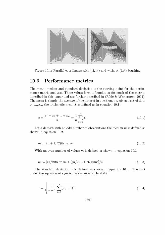
Figure 10.1: Parallel coordinates with (right) and without (left) brushing

10.6 Performance metrics

The mean, median and standard deviation is the starting point for the perfor-mance metric analysis. These values form a foundation for much of the metricsdescribed in this paper and are further described in (Rade & Westergren, 2004).The mean is simply the average of the dataset in question, i.e. given a set of dataxi, ..., xn, the arithmetic mean x is defined as in equation 10.1.

x =x1 + x2 + ...+ xn

n=

1

n

n∑1=n

xi (10.1)

For a dataset with an odd number of observations the median m is defined asshown in equation 10.2.

m := (n+ 1)/2)th value (10.2)

With an even number of values m is defined as shown in equation 10.3.

m := [(n/2)th value + ((n/2) + 1)th value]/2 (10.3)

The standard deviation σ is defined as shown in equation 10.4. The partunder the square root sign is the variance of the data.

σ =

√√√√ 1

n− 1

n∑i=1

(xi − x)2 (10.4)

156

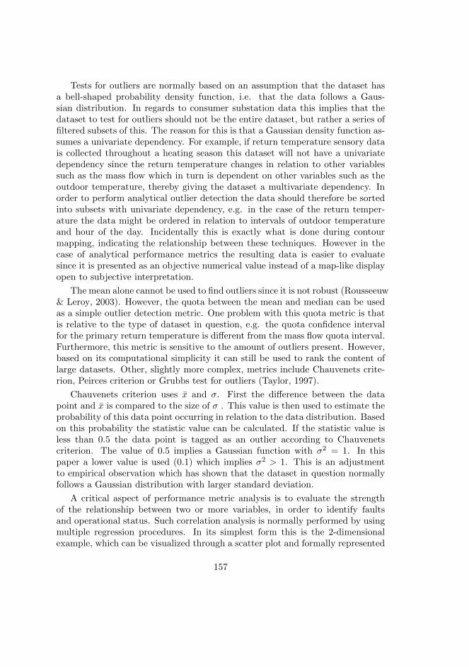
Tests for outliers are normally based on an assumption that the dataset hasa bell-shaped probability density function, i.e. that the data follows a Gaus-sian distribution. In regards to consumer substation data this implies that thedataset to test for outliers should not be the entire dataset, but rather a series offiltered subsets of this. The reason for this is that a Gaussian density function as-sumes a univariate dependency. For example, if return temperature sensory datais collected throughout a heating season this dataset will not have a univariatedependency since the return temperature changes in relation to other variablessuch as the mass flow which in turn is dependent on other variables such as theoutdoor temperature, thereby giving the dataset a multivariate dependency. Inorder to perform analytical outlier detection the data should therefore be sortedinto subsets with univariate dependency, e.g. in the case of the return temper-ature the data might be ordered in relation to intervals of outdoor temperatureand hour of the day. Incidentally this is exactly what is done during contourmapping, indicating the relationship between these techniques. However in thecase of analytical performance metrics the resulting data is easier to evaluatesince it is presented as an objective numerical value instead of a map-like displayopen to subjective interpretation.

The mean alone cannot be used to find outliers since it is not robust (Rousseeuw& Leroy, 2003). However, the quota between the mean and median can be usedas a simple outlier detection metric. One problem with this quota metric is thatis relative to the type of dataset in question, e.g. the quota confidence intervalfor the primary return temperature is different from the mass flow quota interval.Furthermore, this metric is sensitive to the amount of outliers present. However,based on its computational simplicity it can still be used to rank the content oflarge datasets. Other, slightly more complex, metrics include Chauvenets crite-rion, Peirces criterion or Grubbs test for outliers (Taylor, 1997).

Chauvenets criterion uses x and σ. First the difference between the datapoint and x is compared to the size of σ . This value is then used to estimate theprobability of this data point occurring in relation to the data distribution. Basedon this probability the statistic value can be calculated. If the statistic value isless than 0.5 the data point is tagged as an outlier according to Chauvenetscriterion. The value of 0.5 implies a Gaussian function with σ2 = 1. In thispaper a lower value is used (0.1) which implies σ2 > 1. This is an adjustmentto empirical observation which has shown that the dataset in question normallyfollows a Gaussian distribution with larger standard deviation.

A critical aspect of performance metric analysis is to evaluate the strengthof the relationship between two or more variables, in order to identify faultsand operational status. Such correlation analysis is normally performed by usingmultiple regression procedures. In its simplest form this is the 2-dimensionalexample, which can be visualized through a scatter plot and formally represented

157

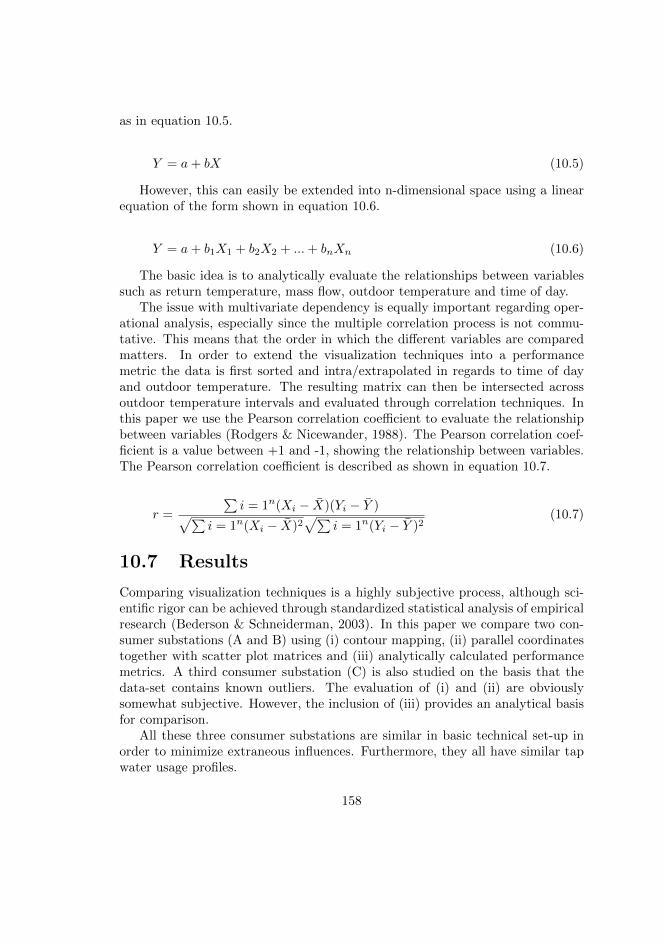
as in equation 10.5.

Y = a+ bX (10.5)

However, this can easily be extended into n-dimensional space using a linearequation of the form shown in equation 10.6.

Y = a+ b1X1 + b2X2 + ...+ bnXn (10.6)

The basic idea is to analytically evaluate the relationships between variablessuch as return temperature, mass flow, outdoor temperature and time of day.

The issue with multivariate dependency is equally important regarding oper-ational analysis, especially since the multiple correlation process is not commu-tative. This means that the order in which the different variables are comparedmatters. In order to extend the visualization techniques into a performancemetric the data is first sorted and intra/extrapolated in regards to time of dayand outdoor temperature. The resulting matrix can then be intersected acrossoutdoor temperature intervals and evaluated through correlation techniques. Inthis paper we use the Pearson correlation coefficient to evaluate the relationshipbetween variables (Rodgers & Nicewander, 1988). The Pearson correlation coef-ficient is a value between +1 and -1, showing the relationship between variables.The Pearson correlation coefficient is described as shown in equation 10.7.

r =

∑i = 1n(Xi − X)(Yi − Y )√∑

i = 1n(Xi − X)2√∑

i = 1n(Yi − Y )2(10.7)

10.7 Results

Comparing visualization techniques is a highly subjective process, although sci-entific rigor can be achieved through standardized statistical analysis of empiricalresearch (Bederson & Schneiderman, 2003). In this paper we compare two con-sumer substations (A and B) using (i) contour mapping, (ii) parallel coordinatestogether with scatter plot matrices and (iii) analytically calculated performancemetrics. A third consumer substation (C) is also studied on the basis that thedata-set contains known outliers. The evaluation of (i) and (ii) are obviouslysomewhat subjective. However, the inclusion of (iii) provides an analytical basisfor comparison.

All these three consumer substations are similar in basic technical set-up inorder to minimize extraneous influences. Furthermore, they all have similar tapwater usage profiles.

158

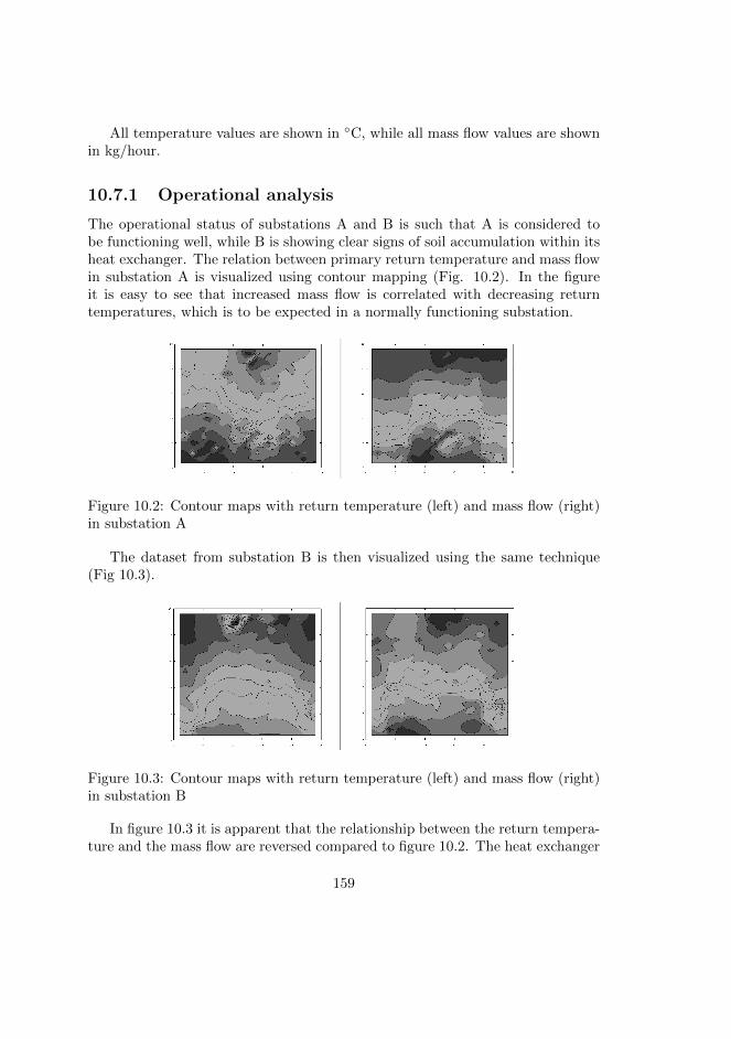
All temperature values are shown in ◦C, while all mass flow values are shownin kg/hour.

10.7.1 Operational analysis

The operational status of substations A and B is such that A is considered tobe functioning well, while B is showing clear signs of soil accumulation within itsheat exchanger. The relation between primary return temperature and mass flowin substation A is visualized using contour mapping (Fig. 10.2). In the figureit is easy to see that increased mass flow is correlated with decreasing returntemperatures, which is to be expected in a normally functioning substation.

Figure 10.2: Contour maps with return temperature (left) and mass flow (right)in substation A

The dataset from substation B is then visualized using the same technique(Fig 10.3).

Figure 10.3: Contour maps with return temperature (left) and mass flow (right)in substation B

In figure 10.3 it is apparent that the relationship between the return tempera-ture and the mass flow are reversed compared to figure 10.2. The heat exchanger

159

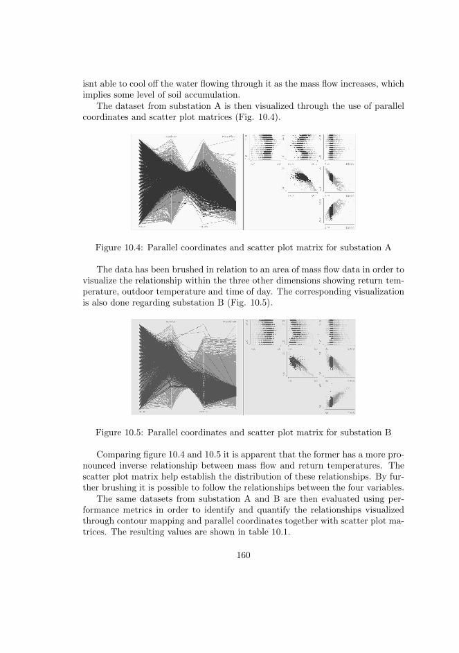
isnt able to cool off the water flowing through it as the mass flow increases, whichimplies some level of soil accumulation.

The dataset from substation A is then visualized through the use of parallelcoordinates and scatter plot matrices (Fig. 10.4).

Figure 10.4: Parallel coordinates and scatter plot matrix for substation A

The data has been brushed in relation to an area of mass flow data in order tovisualize the relationship within the three other dimensions showing return tem-perature, outdoor temperature and time of day. The corresponding visualizationis also done regarding substation B (Fig. 10.5).

Figure 10.5: Parallel coordinates and scatter plot matrix for substation B

Comparing figure 10.4 and 10.5 it is apparent that the former has a more pro-nounced inverse relationship between mass flow and return temperatures. Thescatter plot matrix help establish the distribution of these relationships. By fur-ther brushing it is possible to follow the relationships between the four variables.

The same datasets from substation A and B are then evaluated using per-formance metrics in order to identify and quantify the relationships visualizedthrough contour mapping and parallel coordinates together with scatter plot ma-trices. The resulting values are shown in table 10.1.

160

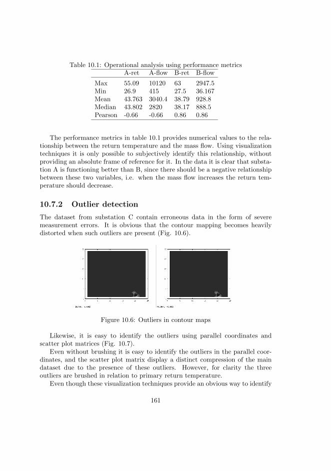
Table 10.1: Operational analysis using performance metricsA-ret A-flow B-ret B-flow

Max 55.09 10120 63 2947.5Min 26.9 415 27.5 36.167Mean 43.763 3040.4 38.79 928.8Median 43.802 2820 38.17 888.5Pearson -0.66 -0.66 0.86 0.86

The performance metrics in table 10.1 provides numerical values to the rela-tionship between the return temperature and the mass flow. Using visualizationtechniques it is only possible to subjectively identify this relationship, withoutproviding an absolute frame of reference for it. In the data it is clear that substa-tion A is functioning better than B, since there should be a negative relationshipbetween these two variables, i.e. when the mass flow increases the return tem-perature should decrease.

10.7.2 Outlier detection

The dataset from substation C contain erroneous data in the form of severemeasurement errors. It is obvious that the contour mapping becomes heavilydistorted when such outliers are present (Fig. 10.6).

Figure 10.6: Outliers in contour maps

Likewise, it is easy to identify the outliers using parallel coordinates andscatter plot matrices (Fig. 10.7).

Even without brushing it is easy to identify the outliers in the parallel coor-dinates, and the scatter plot matrix display a distinct compression of the maindataset due to the presence of these outliers. However, for clarity the threeoutliers are brushed in relation to primary return temperature.

Even though these visualization techniques provide an obvious way to identify

161

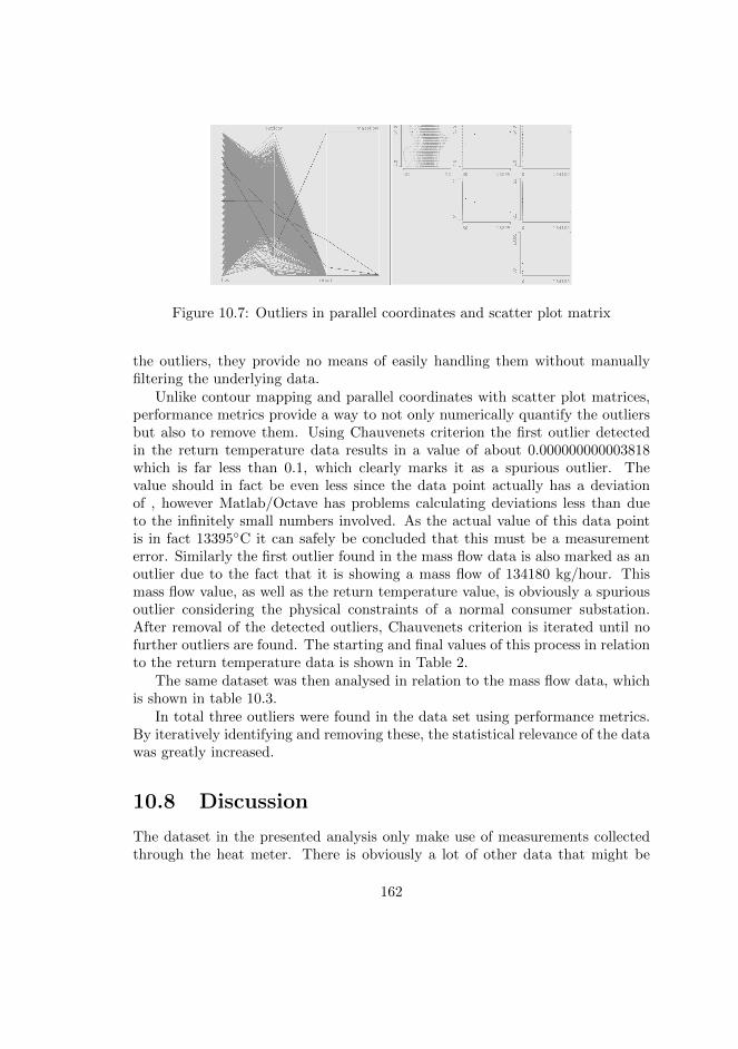
Figure 10.7: Outliers in parallel coordinates and scatter plot matrix

the outliers, they provide no means of easily handling them without manuallyfiltering the underlying data.

Unlike contour mapping and parallel coordinates with scatter plot matrices,performance metrics provide a way to not only numerically quantify the outliersbut also to remove them. Using Chauvenets criterion the first outlier detectedin the return temperature data results in a value of about 0.000000000003818which is far less than 0.1, which clearly marks it as a spurious outlier. Thevalue should in fact be even less since the data point actually has a deviationof , however Matlab/Octave has problems calculating deviations less than dueto the infinitely small numbers involved. As the actual value of this data pointis in fact 13395◦C it can safely be concluded that this must be a measurementerror. Similarly the first outlier found in the mass flow data is also marked as anoutlier due to the fact that it is showing a mass flow of 134180 kg/hour. Thismass flow value, as well as the return temperature value, is obviously a spuriousoutlier considering the physical constraints of a normal consumer substation.After removal of the detected outliers, Chauvenets criterion is iterated until nofurther outliers are found. The starting and final values of this process in relationto the return temperature data is shown in Table 2.

The same dataset was then analysed in relation to the mass flow data, whichis shown in table 10.3.

In total three outliers were found in the data set using performance metrics.By iteratively identifying and removing these, the statistical relevance of the datawas greatly increased.

10.8 Discussion

The dataset in the presented analysis only make use of measurements collectedthrough the heat meter. There is obviously a lot of other data that might be

162

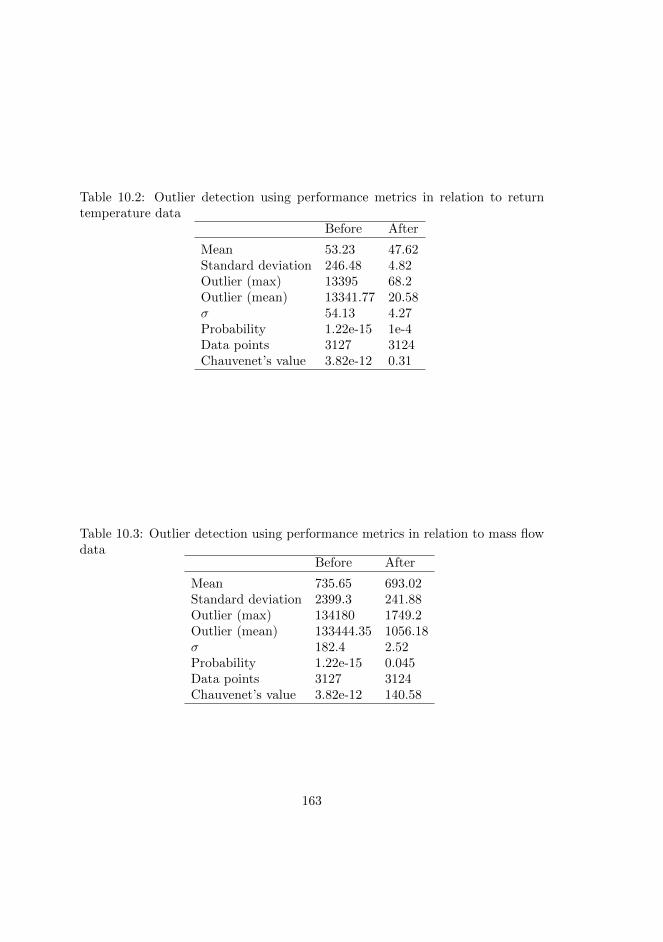
Table 10.2: Outlier detection using performance metrics in relation to returntemperature data

Before After

Mean 53.23 47.62Standard deviation 246.48 4.82Outlier (max) 13395 68.2Outlier (mean) 13341.77 20.58σ 54.13 4.27Probability 1.22e-15 1e-4Data points 3127 3124Chauvenet’s value 3.82e-12 0.31

Table 10.3: Outlier detection using performance metrics in relation to mass flowdata

Before After

Mean 735.65 693.02Standard deviation 2399.3 241.88Outlier (max) 134180 1749.2Outlier (mean) 133444.35 1056.18σ 182.4 2.52Probability 1.22e-15 0.045Data points 3127 3124Chauvenet’s value 3.82e-12 140.58

163

interesting to include in the analysis, such as indoor temperatures, heating systemdata or tap water usage. The reason that only data from the heat meter is usedis simply because this data is readily available to the energy company.

It should be noted that contour maps and parallel coordinates differ in oneimportant regard. A contour map requires extra-/interpolation in order to work.This is due to the fact that array structures are turned into matrices. Thisnot only requires considerable amount of computing power, but is also prone toerror since no existing algorithm can guarantee truth. On the other hand, avisualization solution based on parallel coordinates will only use the unspoiledraw data set.

The main advantage of using parallel coordinates and scatter plot matricescompared to contour maps is that they facilitate the study of multivariate rela-tionships in one visualization artefact. The importance of this only increases asmore variables are introduced into the analysis.

An important aspect of parallel coordinates is the use of brushing. Contourmapping requires no such manipulation during use since they are fixed. However,it can be argued that this is actually an advantage for parallel coordinates sinceit facilities the possibility to angle the visualization in the desired direction andto compare and highlight different aspects of the dataset.

In regards to visualization contour maps have an advantage in that they arerelated to the time of day over the x-axis, which might make it more directlyaccessible. Brushing has to be used in order to analyze hourly dependencies usingparallel coordinates. This might be done by brushing high mass flow values andstudying their relationship with the hour-data. With scatter plot matrices thisprocess is easier since the row of matrices relating to hours basically correlatesto a contour map.

It can be noted that contour maps as well as parallel coordinates and scatterplot matrices are sensitive to outliers. Statistically this is due to compression ofthe dataset, which causes heavy distortion when visualized. Using performancemetrics outliers will instead result in different numerical values which serve tonot only to identify the presence of outliers but also facilitate their ranking andpossible removal.

Given a group of consumer substations it is easier to evaluate their operationalstatus using a list of sorted numbers than maps or graphs. This supports theconclusion that performance metrics are superior to visualization techniques whenevaluating larger groups of substations, and certainly if the evaluation process isto be automated.

164

10.9 Conclusions

In this paper we have compared contour mapping with parallel coordinates andscatter plot matrices in relation to fault detection and operational analysis inconsumer substations within a district heating system. It is shown that the sameoperational relationships can be visualized using parallel coordinates and scatterplot matrices as in contour mapping, while at the same time decreasing thecomputational complexity and error sensitivity and enhancing the multivariateanalysis.

We have also studied the possibilities of using performance metrics as a basisfor large-scale operational analysis within district heating systems. Performancemetrics is an extension of the previously discussed visualization techniques inthat they remove the need for subjective interpretation. It is shown that suchstatistical analysis is able to detect, identify and analytically evaluate the samerelationships studied in relation to the visualization techniques.

10.10 Future work

The focus of this paper was to study data collected through the heat meter. In thefuture other data will be included in the analysis in order to develop a completemodel of the operational status, not only of the consumer substation, but ratherthe whole building in relation to indoor climate and energy saving measures. Thiswork is expected to intensify as the amount of available data increases throughprogress in communication and sensory equipment (Gustafsson, 2011).

Furthermore, the performance metrics analysis will be extended end enhancedin order to facilitate large-scale fault detection and operational analysis. As theoperational constraints harden for most energy companies it becomes increasinglyinteresting for them to help building-owners manage their consumer substationsas smoothly as possible.

10.11 Acknowledgement

The authors would like to thank Dr. Stefan Axelsson at Blekinge Institute ofTechnology for valuable discussions regarding visualization techniques.

We thank NODA Intelligent Systems AB for the use of operational data.

165

166

Chapter 11

Paper X - Distributedthermal storage usingmultiagent systems

Thermal storage is an essential concept within many energy systems. Such stor-age is generally used in order to smooth out the time lag between the acquisitionand the use of energy, for example by using heat water tanks within heating sys-tems. In this work we use a multi-agent system in order to maintain and operatedistributed thermal storage among a large group of buildings in a district heat-ing system. There are several financial and environmental benefits of using sucha system, such as avoiding peak load production, optimizing combined heat andpower strategies and achieving general energy efficiency within the network.

Normally a district heating system is purely demand driven, resulting in pooroperational characteristics on a system wide scale. However, by using the thermalinertia of buildings it is possible to manage and coordinate the heat load among alarge group of buildings in order to implement supply driven operational strategies.This results in increased possibilities to optimize the production mix from financialand environmental aspects.

In this paper we present a multi-agent system which combines the thermal stor-age capacities within buildings in relation to production optimization strategies.The agent system consist of producer agents responsible for valuing the necessaryheat load management, consumer agents managing the quality of service in in-dividual buildings while consenting to participate in heat load management anda market agent acting as a mediating layer between the producer and consumeragents. The market agent uses an auction-like process in order to coordinate the

167

heat load management among the consumer agents, while the producer agentsuse load forecasting in order to evaluate the need for heat load management atany given point in time. A consumer agent uses continues feedback regarding in-door climate in order to uphold quality of service while participating in heat loadmanagement.

Real-time data from a district heating system in Sweden is used in order toevaluate the agent system in relation to operational peak load management. Theresults show clear financial and environmental gains for the producer as well asparticipating consumers.

11.1 Introduction

This paper describes a multi-agent system used in order to improve the opera-tional management of a district heating system in relation to financial and en-vironmental aspects. District heating and cooling is an integrated part of theenergy infrastructure in many countries. This is especially true in Northern andEastern Europe, although district heating and cooling is growing rapidly in pop-ularity around the world [1]. A district heating system consists of one or moreproduction units which distribute heated water or steam throughout at pipe net-work. Buildings are then connected to this network, usually through the meansof heat exchangers which transfer the heat to the heating- and tap water systemin the building. District heating systems are often considered environmentallyand financially sound, since the centralized set-up facilitates large scale energyefficiency schemes. More or less any type of production units can be used in a dis-trict heating system, and the fuels used range from biomass and industrial wasteheat to coal and oil. Many district heating systems also make use of combinedheat and power production (CHP) which have a very high level of utilization ofthe primary fuel used [2]. A CHP plant produces electrical power at the sametime as it heats the water for the district heating system. First water is boiledinto steam which is used in order to run a turbine, which in turn is connected to agenerator which converts the mechanical energy to electrical energy. Afterwardsthe steam is passed through a condensing unit which transfers the heat to thedistrict heating system. As the steam cools off it can be re-heated before beingpassed into the turbine again. A traditional power plant has an energy efficiencyof about 30-50%, while a CHP plant utilizes about 80-90% of the primary fuel.The electricity produced in the CHP plant is then sold on the power market whilethe heat is being sold within the connected district heating system.

Normally a district heating system is purely demand driven, in the sensethat the production units can only react to the current heat demand within thenetwork. The bulk of the heat demand consist of demand for building heating,although substantial heat load peaks are also generated by social patterns in

168

relation to tap water usage. The heating demand in a building is correlatedto the outdoor temperature, while tap water usage is more correlated to time ofday. This combination of outdoor temperature dependencies and social behaviourover the day causes fluctuations in the heat demand. Such fluctuations or heatload peaks are very undesirable for a number of reasons. Most district heatingsystems have a production set-up using some sort of base load boilers which arecomplemented with a range of peak load boilers. The base load boilers are oftenfuelled by cheap and environmentally friendly fuels such as biomass or industrialwaste heat, while the peak load boilers normally use fossil fuels such as oil or gaswhich are not only expensive but also generate undesirable emissions.

In this paper we describe a multi-agent system which uses the thermal in-ertia of buildings in order to manage the heat load demand in relation to theoperational status at the production units. By managing the demand in such away it is possible to make the district heating system more supply driven, i.e.it is possible to optimize the heat load usage in relation to the production sta-tus and not only the other way around. This is similar to using large storagetanks, although here the thermal inertia of the connected buildings is used as adistributed storage instead. By using such a set-up it is possible to shed heatload peaks in order to avoid using peak load boilers, or to move the heat loadpeaks in time in order to coordinate the heat load peaks with high spot pricesfor electricity when using CHP. The use of large storage tanks is well understoodand is a mature technique within district heating systems, and similar strategiesare possible to utilize with the proposed distributed thermal storage [3].

The multi-agent system consists of three different agent entities; the produceragent, the consumer agent and the market agent. This paper focuses on themarket agent component which acts as a mediating layer between the consumerand producer agents. The market agent uses as an auction-like process in orderto coordinate heat load demand among the consumer agents in relation to theoperational status of the producer agents.

The paper starts off by describing related and previous work concerning multi-agent based heat load management within district heating systems. In sectionthree the physical process of managing the heat load usage in relation to thermalinertia of a building structure is discussed. Section four presents the functionalityof the coordination process within the multi-agent system. Section five describesthe experimental set-up used in evaluating the system, and the results are pre-sented and discussed in sections six and seven. Finally the paper is concluded insection eight and nine with conclusions and future work.

169

11.2 Related work

The framework for the multi-agent systems is built around three different agenttypes; the consumer agents, the producer agents and the market agent used tocoordinate the interaction between the two former agent groups. This basic set-up was first introduced in a previous paper [4], and has since been expanded tocover the practical issues present in a real-time industrial setting [5]. The last fewyears the system has matured through a series of industrial installations showingthe potential of the concept in operational settings [6]. Lately the theoreticalfoundation for the system has been refined through work considering the pro-ducer and consumer agent entities. An optimization algorithm for coordinatingthe desired heat load in relation to operational constraints was presented in a re-cent paper [7]. Together with heat load forecasting algorithms such optimizationalgorithms are used as decision support tools by the producer agents when cal-culating their desired future state. Heat load forecasts are produced by relatinghistorical operational data of the district heating system with forecasts of the out-door temperature, in combination with estimations of social behaviour affectingtap water usage and ventilation. Such systems have been studied extensively inprevious papers [8] and [9]. More complex solutions use seasonal autoregressiveintegrated moving averages [10], or basic Box-Jenkins autoregressive integratedmoving averages [11] and [12]. Other approaches for heat load forecasting includea grey-box process explicitly using climate data to forecast heat consumption ina large geographical area [13].

The consumer agent tries to balance the ability to partake in load control whilesimultaneously upholding required levels of quality of service (QoS). The conceptof quality filters was proposed in [14]. This concept is based on the idea that theconsumer agent should be responsible for the QoS in the building by means ofcontinues measuring and evaluation, thus being able to take informed decisionsregarding participation in any requested load control. Maintaining a sufficientlevel of QoS is at the core of any heating or cooling strategy, and a consumeragent must only act within the constraints set by hereby. An energy balancemodel for large-scale QoS evaluation within a multi-agent system was presentedin [15]. The focus of [15] and [7] was on the specific application of combinedheat and power generation while this paper combines the conceptual foundationfor producer and consumer agents with a framework for a general application ofdistributed thermal storage by extending the market agent process.

The basic process of using heat storage facilities within buildings in order toimprove the operational functionality of a district heating system has been previ-ously studied in [16] and [17]. The ability to do this on a large scale throughoutan entire district heating network was evaluated and quantified in [18], and fur-ther studies on the process of storing heat in building structures are presented in

170

[19]. The process of pre-cooling and demand limiting in relation to this has beenstudied in several studies such as [20] and [21]. Basic heating control strategiesare presented in [22], while more complex adaptive strategies are presented in [23]and [24]. All these strategies make use of the thermal inertia within the buildingstructures in order to improve the heating and/or cooling demand.

An early attempt on demand side management was presented during the1980s. And although the current hardware and communication capabilities lim-ited the operational functionality of the proposed system, the future potential ofthe system was apparent [25]. It should be noted that the importance of two-waycommunication in order to enable feedback was acknowledged even in these earlyworks [26].

11.3 Multi-agent system overview

The multi-agent system uses three different main types of agents in order to dis-tribute and coordinate the heat load among the participating buildings; produceragents, consumer agents and market agents. A producer agent will work to opti-mize its operational production in regards to fuel prices in the general case andpower market spot prices in the case of combined heat and power generation.Such operational management is done by distributed heat storage among build-ings connected to the district heating network. Whenever the producer agentdeems it necessary to perform heat load management it will request load controlamong the consumer agents. The producer agent will have to pay the partici-pating consumer agents so it is important for the producer agent to set the priceconstraints correctly. The coordination of this load control between the consumerand production agents is done by the market agent.

The agents are controlled by an implicit norm system in which agents areassumed not to cheat or lie. Specifically, in order to avoid collusive behaviourthe agents are not permitted to form coalitions. A consumer agent is assumedto be truthful regarding its internal energy balance status, i.e. it is assumedthat a building owner doesnt want the residents to complain about the indoortemperature. Furthermore, in multi-producer agent settings it is assumed thatthe producer agents will not impose on load management instigated by otherproducer agents, although they have the information to do this based on theon-line auction status.

An energy company and all its production units are represented by a produceragent. Most district heating systems are run by one single energy company, butthere could also be several energy companies competing within a network. In thecase of a single energy company the producer agent will only need to consider itsown operational constraints, while in a multi-energy company setting it will alsoneed to perform real-time evaluation in regards to the status of its competitors.

171

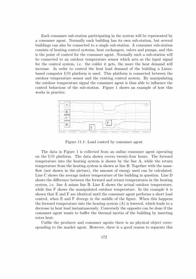
Each consumer sub-station participating in the system will be represented bya consumer agent. Normally each building has its own sub-station, but severalbuildings can also be connected to a single sub-station. A consumer sub-stationconsists of heating control systems, heat exchangers, valves and pumps, and thisis the point of control for the consumer agent. Normally such a sub-station willbe connected to an outdoor temperature sensor which acts as the input signalfor the control system, i.e. the colder it gets, the more the heat demand willincrease. In order to control the heat load demand of the building a Linux-based computer I/O platform is used. This platform is connected between theoutdoor temperature sensor and the existing control system. By manipulatingthe outdoor temperature signal the consumer agent is thus able to influence thecontrol behaviour of the sub-station. Figure 1 shows an example of how thisworks in practice.

Figure 11.1: Load control by consumer agent

The data in Figure 1 is collected from an online consumer agent operatingon the I/O platform. The data shown covers twenty-four hours. The forwardtemperature into the heating system is shown by the line A, while the returntemperature from the heating system is shown at line B. Together with the mass-flow (not shown in the picture), the amount of energy used can be calculated.Line C shows the average indoor temperature of the building in question. Line Dshows the difference between the forward and return temperatures in the heatingsystem, i.e. line A minus line B. Line E shows the actual outdoor temperature,while line F shows the manipulated outdoor temperature. In the example it isshown that E and F are identical until the consumer agent performs a short loadcontrol, when E and F diverge in the middle of the figure. When this happensthe forward temperature into the heating system (A) is lowered, which leads to adecrease in heat load instantaneously. Conversely the opposite can be done if theconsumer agent wants to buffer the thermal inertia of the building by insertingextra heat.

Unlike the producer and consumer agents there is no physical object corre-sponding to the market agent. However, there is a good reason to separate this

172

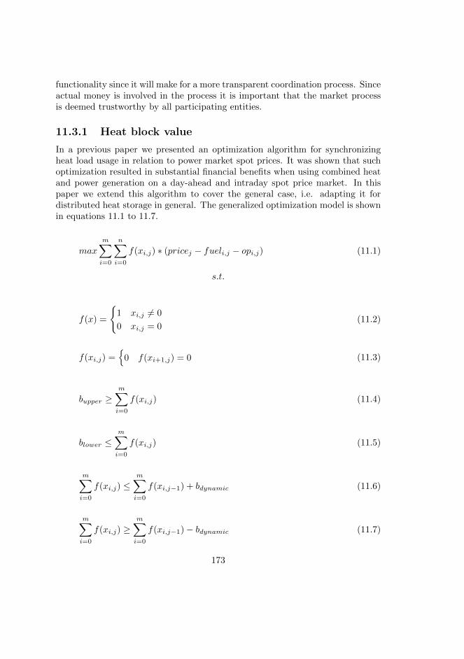
functionality since it will make for a more transparent coordination process. Sinceactual money is involved in the process it is important that the market processis deemed trustworthy by all participating entities.

11.3.1 Heat block value

In a previous paper we presented an optimization algorithm for synchronizingheat load usage in relation to power market spot prices. It was shown that suchoptimization resulted in substantial financial benefits when using combined heatand power generation on a day-ahead and intraday spot price market. In thispaper we extend this algorithm to cover the general case, i.e. adapting it fordistributed heat storage in general. The generalized optimization model is shownin equations 11.1 to 11.7.

max

m∑i=0

n∑i=0

f(xi,j) ∗ (pricej − fueli,j − opi,j) (11.1)

s.t.

f(x) =

{1 xi,j 6= 0

0 xi,j = 0(11.2)

f(xi,j) ={

0 f(xi+1,j) = 0 (11.3)

bupper ≥m∑i=0

f(xi,j) (11.4)

blower ≤m∑i=0

f(xi,j) (11.5)

m∑i=0

f(xi,j) ≤m∑i=0

f(xi,j−1) + bdynamic (11.6)

m∑i=0

f(xi,j) ≥m∑i=0

f(xi,j−1)− bdynamic (11.7)

173

Equation 11.1 maximises the total earnings. The value of sold heat can onlychange from hour to hour, while the cost for producing the heat can changeboth in time and in relation to the level of heat load demand. The costs areseparated in fuel costs and operational costs. Such operational costs include costsfor starting and shutting down boiler and costs related to managing the boilers.An m by n matrix represents the heat load demand during a time period, wherem is the theoretical maximum amount of heat load in the system. The valueof n is normally 24, i.e. the head load demand is evaluated one day ahead andis discretizised into hours. Equations 11.2-11.7 define the operational boundaryconditions for the optimization model.

An optimization model for production is dependent on heat load forecastsranging from hours to a few days ahead. Such forecasts are calculated basedon a combination of previous operational data and weather forecasts. The mainparameter from the weather forecast to consider is the outdoor temperature,although general weather conditions such as precipitation and wind affect thesituation to some extent. Using the heat load forecasts a producer agent canarrange the wanted heat load demand hour by hour in relation to fuel prices andother related costs. By doing this it is possible to minimize the use of expensiveand environmentally unsound peak load fuels. In order to make the model usefulin practice the heat load demand represented by a matrix which is discretizisedinto blocks. Each such block is called a heat block, and it is these heat blocks thatthe producer agent will sell to the consumer agents through the market process.

A heat block represents a certain monetary value for the producer agent, sinceif the consumer agents successfully implement the load control specified by theheat block this will translate into an improved operational status at the physicalproduction units. However, some of these added earnings will have to be used topay the consumer agents participating in managing the heat load demand withineach heat block. Based on the optimization model the producer agent will beable to evaluate the financial value for heat block, and will thus be able to set amaximum price it is willing to pay for the implementation of the associated loadcontrol. The producer agent is also able to set the size for the heat blocks basedon the boundary conditions in the optimization model, i.e. the size of the matrixis based on the operational conditions within the production units.

11.3.2 Consumer agent asset

The consumer agents get paid by the producer agents in order to perform loadcontrol. The payments are accumulated during the payment period, usually amonth, and then subtracted from the heating bill. Obviously a consumer agentwould want to maximize this revenue, by performing as much load control aspossible. At the same time the consumer agent is responsible for maintaining

174

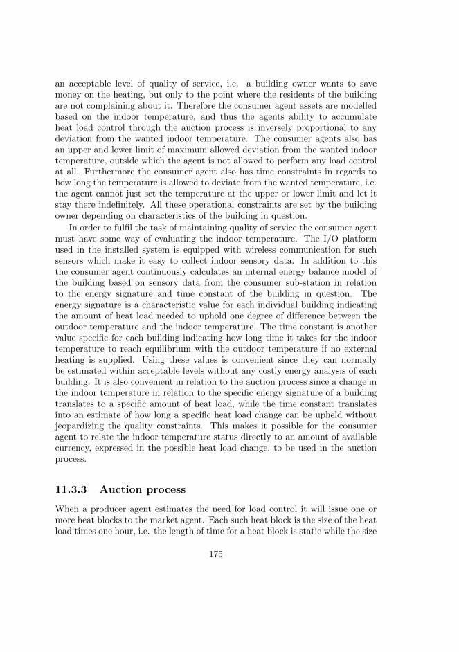
an acceptable level of quality of service, i.e. a building owner wants to savemoney on the heating, but only to the point where the residents of the buildingare not complaining about it. Therefore the consumer agent assets are modelledbased on the indoor temperature, and thus the agents ability to accumulateheat load control through the auction process is inversely proportional to anydeviation from the wanted indoor temperature. The consumer agents also hasan upper and lower limit of maximum allowed deviation from the wanted indoortemperature, outside which the agent is not allowed to perform any load controlat all. Furthermore the consumer agent also has time constraints in regards tohow long the temperature is allowed to deviate from the wanted temperature, i.e.the agent cannot just set the temperature at the upper or lower limit and let itstay there indefinitely. All these operational constraints are set by the buildingowner depending on characteristics of the building in question.

In order to fulfil the task of maintaining quality of service the consumer agentmust have some way of evaluating the indoor temperature. The I/O platformused in the installed system is equipped with wireless communication for suchsensors which make it easy to collect indoor sensory data. In addition to thisthe consumer agent continuously calculates an internal energy balance model ofthe building based on sensory data from the consumer sub-station in relationto the energy signature and time constant of the building in question. Theenergy signature is a characteristic value for each individual building indicatingthe amount of heat load needed to uphold one degree of difference between theoutdoor temperature and the indoor temperature. The time constant is anothervalue specific for each building indicating how long time it takes for the indoortemperature to reach equilibrium with the outdoor temperature if no externalheating is supplied. Using these values is convenient since they can normallybe estimated within acceptable levels without any costly energy analysis of eachbuilding. It is also convenient in relation to the auction process since a change inthe indoor temperature in relation to the specific energy signature of a buildingtranslates to a specific amount of heat load, while the time constant translatesinto an estimate of how long a specific heat load change can be upheld withoutjeopardizing the quality constraints. This makes it possible for the consumeragent to relate the indoor temperature status directly to an amount of availablecurrency, expressed in the possible heat load change, to be used in the auctionprocess.

11.3.3 Auction process

When a producer agent estimates the need for load control it will issue one ormore heat blocks to the market agent. Each such heat block is the size of the heatload times one hour, i.e. the length of time for a heat block is static while the size

175

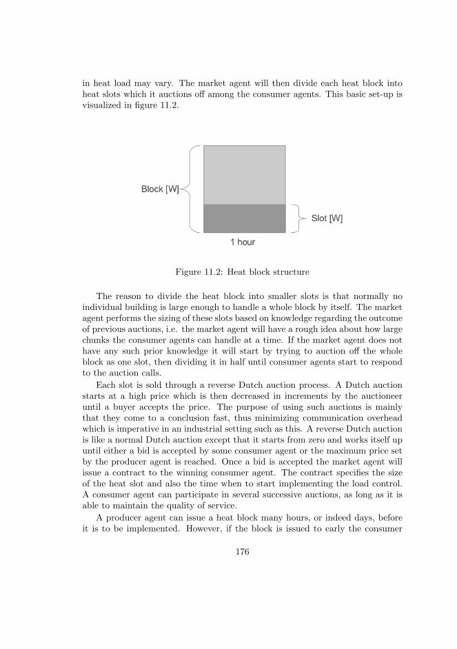
in heat load may vary. The market agent will then divide each heat block intoheat slots which it auctions off among the consumer agents. This basic set-up isvisualized in figure 11.2.

Figure 11.2: Heat block structure

The reason to divide the heat block into smaller slots is that normally noindividual building is large enough to handle a whole block by itself. The marketagent performs the sizing of these slots based on knowledge regarding the outcomeof previous auctions, i.e. the market agent will have a rough idea about how largechunks the consumer agents can handle at a time. If the market agent does nothave any such prior knowledge it will start by trying to auction off the wholeblock as one slot, then dividing it in half until consumer agents start to respondto the auction calls.

Each slot is sold through a reverse Dutch auction process. A Dutch auctionstarts at a high price which is then decreased in increments by the auctioneeruntil a buyer accepts the price. The purpose of using such auctions is mainlythat they come to a conclusion fast, thus minimizing communication overheadwhich is imperative in an industrial setting such as this. A reverse Dutch auctionis like a normal Dutch auction except that it starts from zero and works itself upuntil either a bid is accepted by some consumer agent or the maximum price setby the producer agent is reached. Once a bid is accepted the market agent willissue a contract to the winning consumer agent. The contract specifies the sizeof the heat slot and also the time when to start implementing the load control.A consumer agent can participate in several successive auctions, as long as it isable to maintain the quality of service.

A producer agent can issue a heat block many hours, or indeed days, beforeit is to be implemented. However, if the block is issued to early the consumer

176

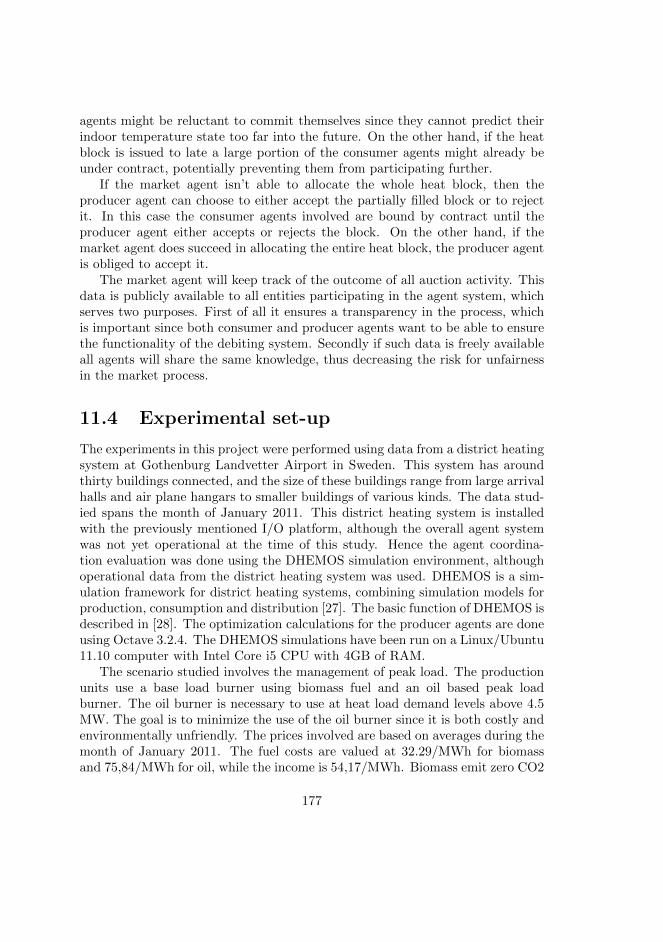
agents might be reluctant to commit themselves since they cannot predict theirindoor temperature state too far into the future. On the other hand, if the heatblock is issued to late a large portion of the consumer agents might already beunder contract, potentially preventing them from participating further.

If the market agent isn’t able to allocate the whole heat block, then theproducer agent can choose to either accept the partially filled block or to rejectit. In this case the consumer agents involved are bound by contract until theproducer agent either accepts or rejects the block. On the other hand, if themarket agent does succeed in allocating the entire heat block, the producer agentis obliged to accept it.

The market agent will keep track of the outcome of all auction activity. Thisdata is publicly available to all entities participating in the agent system, whichserves two purposes. First of all it ensures a transparency in the process, whichis important since both consumer and producer agents want to be able to ensurethe functionality of the debiting system. Secondly if such data is freely availableall agents will share the same knowledge, thus decreasing the risk for unfairnessin the market process.

11.4 Experimental set-up

The experiments in this project were performed using data from a district heatingsystem at Gothenburg Landvetter Airport in Sweden. This system has aroundthirty buildings connected, and the size of these buildings range from large arrivalhalls and air plane hangars to smaller buildings of various kinds. The data stud-ied spans the month of January 2011. This district heating system is installedwith the previously mentioned I/O platform, although the overall agent systemwas not yet operational at the time of this study. Hence the agent coordina-tion evaluation was done using the DHEMOS simulation environment, althoughoperational data from the district heating system was used. DHEMOS is a sim-ulation framework for district heating systems, combining simulation models forproduction, consumption and distribution [27]. The basic function of DHEMOS isdescribed in [28]. The optimization calculations for the producer agents are doneusing Octave 3.2.4. The DHEMOS simulations have been run on a Linux/Ubuntu11.10 computer with Intel Core i5 CPU with 4GB of RAM.

The scenario studied involves the management of peak load. The productionunits use a base load burner using biomass fuel and an oil based peak loadburner. The oil burner is necessary to use at heat load demand levels above 4.5MW. The goal is to minimize the use of the oil burner since it is both costly andenvironmentally unfriendly. The prices involved are based on averages during themonth of January 2011. The fuel costs are valued at 32.29/MWh for biomassand 75,84/MWh for oil, while the income is 54,17/MWh. Biomass emit zero CO2

177

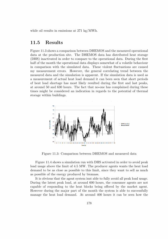
while oil results in emissions at 271 kg/MWh.

11.5 Results

Figure 11.3 shows a comparison between DHEMOS and the measured operationaldata at the production site. The DHEMOS data has distributed heat storage(DHS) inactivated in order to compare to the operational data. During the firsthalf of the month the operational data displays somewhat of a volatile behaviourin comparison with the simulated data. These violent fluctuations are causedmy measurement errors. However, the general correlating trend between themeasured data and the simulation is apparent. If the simulation data is used asa measurement of actual heat load demand it can been seen that short periodsof heat load shortage has most likely resulted during the first and last peaks,at around 50 and 630 hours. The fact that no-one has complained during thesetimes might be considered an indication in regards to the potential of thermalstorage within buildings.

Figure 11.3: Comparison between DHEMOS and measured data

Figure 11.4 shows a simulation run with DHS activated in order to avoid peakload usage above the limit of 4.5 MW. The producer agents wants the heat loaddemand to be as close as possible to this limit, since they want to sell as muchas possible of the energy produced by biomass.

It is obvious that the agent system isnt able to fully avoid all peak load usage.During the latest peak load, at around 600 hours, the consumer agents are notcapable of responding to the heat blocks being offered by the market agent.However during the major part of the month the system is able to successfullymanage the heat load demand. At around 400 hours it can be seen how the

178

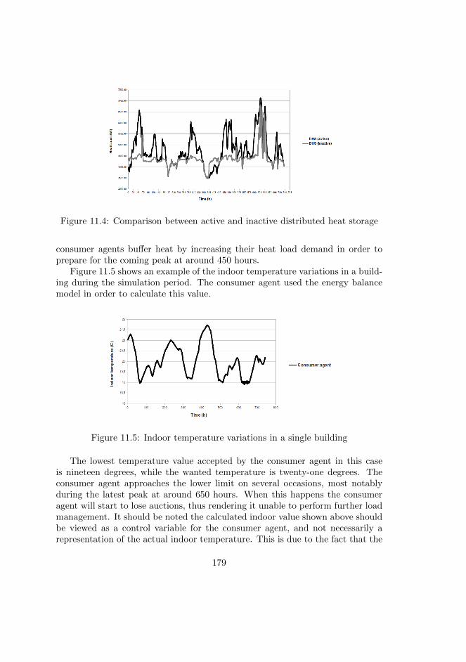
Figure 11.4: Comparison between active and inactive distributed heat storage

consumer agents buffer heat by increasing their heat load demand in order toprepare for the coming peak at around 450 hours.

Figure 11.5 shows an example of the indoor temperature variations in a build-ing during the simulation period. The consumer agent used the energy balancemodel in order to calculate this value.

Figure 11.5: Indoor temperature variations in a single building

The lowest temperature value accepted by the consumer agent in this caseis nineteen degrees, while the wanted temperature is twenty-one degrees. Theconsumer agent approaches the lower limit on several occasions, most notablyduring the latest peak at around 650 hours. When this happens the consumeragent will start to lose auctions, thus rendering it unable to perform further loadmanagement. It should be noted the calculated indoor value shown above shouldbe viewed as a control variable for the consumer agent, and not necessarily arepresentation of the actual indoor temperature. This is due to the fact that the

179

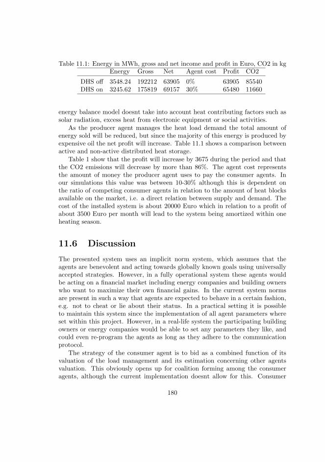
Table 11.1: Energy in MWh, gross and net income and profit in Euro, CO2 in kgEnergy Gross Net Agent cost Profit CO2

DHS off 3548.24 192212 63905 0% 63905 85540DHS on 3245.62 175819 69157 30% 65480 11660

energy balance model doesnt take into account heat contributing factors such assolar radiation, excess heat from electronic equipment or social activities.

As the producer agent manages the heat load demand the total amount ofenergy sold will be reduced, but since the majority of this energy is produced byexpensive oil the net profit will increase. Table 11.1 shows a comparison betweenactive and non-active distributed heat storage.

Table 1 show that the profit will increase by 3675 during the period and thatthe CO2 emissions will decrease by more than 86%. The agent cost representsthe amount of money the producer agent uses to pay the consumer agents. Inour simulations this value was between 10-30% although this is dependent onthe ratio of competing consumer agents in relation to the amount of heat blocksavailable on the market, i.e. a direct relation between supply and demand. Thecost of the installed system is about 20000 Euro which in relation to a profit ofabout 3500 Euro per month will lead to the system being amortized within oneheating season.

11.6 Discussion

The presented system uses an implicit norm system, which assumes that theagents are benevolent and acting towards globally known goals using universallyaccepted strategies. However, in a fully operational system these agents wouldbe acting on a financial market including energy companies and building ownerswho want to maximize their own financial gains. In the current system normsare present in such a way that agents are expected to behave in a certain fashion,e.g. not to cheat or lie about their status. In a practical setting it is possibleto maintain this system since the implementation of all agent parameters whereset within this project. However, in a real-life system the participating buildingowners or energy companies would be able to set any parameters they like, andcould even re-program the agents as long as they adhere to the communicationprotocol.

The strategy of the consumer agent is to bid as a combined function of itsvaluation of the load management and its estimation concerning other agentsvaluation. This obviously opens up for coalition forming among the consumeragents, although the current implementation doesnt allow for this. Consumer

180

agents might want to form coalitions in order to achieve high prices by agreeing towithhold auction bidding and then splitting the proceeds. If a group of consumeragents were successful in rigging the market like this they could achieve morethan the 10-30% profit share they got during the presented experiments.

In regards to the producer agents there is no incentive for them to lower themaximum price below its true valuation, since this would only harm the produceragent itself by depriving it of financially profitable load management.

11.7 Conclusions

In this paper we have presented a multi-agent system for distributed heat storage.It was shown that such a set-up can be used to reduce, and in many instancesremove, the need for financially and environmentally unsound peak load fuelusage. Since the multi-agent system is operationally adaptable it is able to adjustthe heat load demand in relation to actual operational constraints among theproduction units. This makes it possible to increase the net profit for the energycompany even though the total amount of energy being sold is less.

It was shown that the consumer agents will cooperate in load management aslong as they are able to simultaneously uphold their desired quality of service.

The net profit in district heating system in question was increased by about2.5% which translates to a return of investment in less than one heating seasonconsidering the installation costs involved. At the same time the CO2 emissionswere reduced by more than 86% due to the shift in fuel composition.

11.8 Future work

In the future a framework for explicit management of norms will have to be added.This is imperative since the physical entities represented by the agents need tomaintain trust in the system, even when those entities are allowed to set theirown agent parameters. This system should be based on a set of explicit norms orground-rules, which are then managed through a layer of individual trust amongagents coupled with a globally visible reputation system. The market agent willact as the main manager for this system, and will use punishment by exclusionin order to maintain order. Exclusion translates into financial loss, which will actas deterrence for the agents to deviate from the norms.

11.9 Acknowledgements

The authors would like Swedavia for letting us use operational data from thedistrict heating system at Gothenburg Landvetter Airport. Also, we would like

181

to thank NODA Intelligent System for the use of the agent I/O-platform.

182

Chapter 12

Paper XI - A smart heatgrid framework usingintelligent software agents

In this paper we present a coherent system combining the characteristics and per-formance of different aspects of so called smart grids for district heating systems.The system is based on a multi-agent architecture which provides a flexible androbust framework for distributed coordination and interaction between distinct en-tities within dynamic and unpredictable domains such as heat or power grids. Weexamine the system performance in a industrial setting and provide results fromthree different demand side management strategies implemented in the system.It is shown that an increased ability of the system to automatically coordinateproduction and consumption leads to significant benefits on a system wide scaleas well as on a local scale.

12.1 Introduction

In several previous papers we have described and examined the characteristicsand performance of different aspects of so called smart grids for district heatingsystems. In this paper we integrate these aspects together into a coherent sys-tem and detail the theory and practice underpinning this merger and disseminateresults relating to the development and implementation of such a system. Thetheoretical foundation for this system was previously proposed by the authors(Wernstedt et al., 2007). Although the general agent-based framework is stillevident in the current system several developments have been implemented since

183

then, mostly relating to the process of converting theoretical ideas to robust ap-plications capable of handling the practical dynamics and commercial constraintswithin operational district heating systems.

An agent can be seen as an autonomous software entity that can act indepen-dently based on the needs and desires of the agent in relation to the constraints setby the domain which it inhabits. Agents can also act together with other agents inmulti-agent systems, either by competition or cooperation. Multi-agent systemsis a powerful framework for implementing software-based intelligence for handlingdistributed and complex environments and such systems have been successfullyapplied to many industrial systems and robotic applications (Wooldridge, 2002).Since most energy systems in general and district heating systems in particu-lar are by their nature distributed as well as complex we have used multi-agentsystems as a framework in order to implement the smart grid paradigm.

District heating is the most common heating type in urban areas throughoutNorthern and Eastern Europe, although this type of technology is used all overthe world. In Europe district heating is becoming increasingly vital as part ofa long-term sustainable infrastructure for energy, not least in relation to the in-creasing use of combined heat and power production (CHP) (Constinescu, 2007).A district heating system consists of one or several productions units connectedto the customer units through a distribution network. Normally water is used asthe transfer medium although steam is also used in some systems. The heatedwater is normally accessed by the consumer through a substation containing aheat exchanger which transfers the heat into the building heating and tap watersystem. A district heating producer can use basically any heat source able to heatthe water to the desired temperature, normally around 80-120◦C, which makesdistrict heating a versatile system (Fredriksen & Werner, 1993). The energyefficiency of district heating production can be increased by using a combinedheat and power production plant which produces electrical power simultaneouslywith producing the heat. Such a set-up normally involves overheating water intosteam which is used to run a turbine which in turn is connected to a generatorfor producing electricity. The steam is then fed into a condenser unit which de-creases the temperature and pressure of the steam by transferring the heat tothe district heating water. A traditional power plant has a energy efficiency ofabout 30-50% in relation to the primary fuel, while a CHP is capable of achievingefficiency levels of 80-90% (Horlock, 2008).

Even though a district heating system is demand driven there is usually nodirect information link between consumption, distribution and production. Nor-mally these sub-systems are operated independently of each other even thoughthey are intertwined within a confined physical system. The most basic problemis that the production units normally work optimally with an even load whilethe social behaviour of the end-customers give rise to a variable consumer head

184

demand. This results in a disharmony between demand and supply. In the casethat this problem is addressed at all, the traditional approach is to use storagetanks or to use the distribution network itself as a thermal buffer in order tohandle volatile heat demand (Andrepont, 2012). However, a storage tank is justthat; a thermal buffer without any operational dynamic behaviour, and althoughthey can be used to alleviate peak loads to a certain extent, their lack of op-erational dynamic behaviour makes them less suitable for active optimization.However, by implementing systems like the one proposed in this paper it is pos-sible to achieve a framework for more active operational optimization. Thereare a large number of financial and environmental benefits to be had by directlycoordinating the operational behaviour of consumption in relation to distributionand production. This was realised a long time ago and even in the early nineteeneighties experiments were carried out in order to evaluate these ideas in a practi-cal setting (Osterlind, 1982). However, at the time it was also concluded that thecurrent technology in regards to computational and communication performancewas somewhat lacking and that a theoretical framework for handling distributedand dynamic environments in order to maintain quality of service was missing.Since then computational devices and communication solutions have experiencedan exponential development in performance and cost efficiency. An multi agentbased framework for district heating systems was examined in (Wernstedt, 2005)and further developed in (Wernstedt et al., 2007). By utilizing the inherentcharacteristics of a multi-agent system it was possible to provide a architecturalframework for distributed optimization and information sharing while uphold-ing the operational behaviour required by the different actors within the districtheating system. Within this framework we have developed the behaviour of thedifferent agent-based entities in order to coordinate production optimization andconsumer quality of service (C. Johansson, 2010).

12.2 System overview

An agent can be described as a autonomous entity which observes and acts uponits environment and directs its actions towards achieving certain goals. Modellingsystem components as agents generate several benefits since it provides a way ofstructuring applications in complex computational systems with several conflict-ing entities (Wooldridge, 2002). In this case the overall goals for the system is tooptimize the energy usage in relation to financial and operational aspects whilemaintaining an acceptable quality of service. Due to the previously mentioneddisharmony between supply and demand these two goals can sometimes be inconflict. In order to handle this situation the system is modelled as a collectionof individual agents based on three distinct agent types.

185

Producer agent

The task of the producer agent is to optimize the energy generation in relationto financial and environmental aspects. This optimization can be used in sev-eral different situations, such as the previously mentioned peak load avoidancescheme. Other uses include optimization of combined heat and power produc-tion in relation to electricity spot price or distribution optimization related to forexample pressure maintenance or return temperatures within the district heat-ing network. The primary goal of the producer agent is normally to minimizethe production costs given a set of constraints related to the heat load demandin the network and the physical and financial properties of the production anddistribution infrastructure.

A production agent optimization scheme for combined heat and power pro-duction has previously been presented in (C. Johansson et al., 2012a). In thisscheme the production agent coordinates the thermal buffer of a large amount ofbuildings taking into account hourly spot price projections. However, this schemecan be generalized in order to apply to a wide range of basic demand side manage-ment strategies. Normally an energy producer in a district heating system havetwo basic parameters on which to operate; the pressure head in the distributionnetwork and the supply temperature at the production units, basically indicat-ing a totally demand driven system. By using operational load control a thirdparameter is provided to the energy producer since this allows the producer tomanipulate the heat demand within certain constrains rather than just reactingto it. In a traditional optimization setting, i.e. using the two basic parameters,the energy producer will solve the optimization by minimizing in relation towardsproduction costs (Arvastson, 2001). However, given the ability to perform oper-ational load control the energy producer can instead optimize by maximizing inrelation towards earnings. As before the input for the optimization is an hourlyheat load forecast for a day ahead, although instead of rearranging this heat loadarray in relation to spot price it will be arranged according to general earningsin relation to system constraints.

In the spot price-based optimization process the producer agent received dayahead data from external providers, like Nord Pool Spot in Northern Europe.This data could then be used to evaluate the financial value of different heatload levels. In the generalized optimization process the producer agent insteadhas to calculate this financial data based on the operational constraints in theproduction units available in the specific district heating system. It should benoted that the previously mentioned spot price situation can be modelled as suchoperational constraints in the generalized case. The starting point for such ananalysis is a forecast estimating the heat load hour by hour for the coming day.Such heat loads forecasts are normally based on regression analysis of historicaldata (Jonsson, 2002; Dotzauer, 2002), but they can also be based on other types

186

of forecasting techniques such as time series analysis (Grosswindhager et al., 2011;Box & G.M., 1991; Chramcov et al., 2009) and neural networks (Kato, Sakawa,Ishimaru, Ushiro, & Shibano, 2008).

The heat load forecast is considered to be the representation of what willhappen if no operational load control is performed, i.e. the situation in thenormal production cost minimization case. However, incorporating the systemsability to perform load control in the constraints for the optimization modelenables the possibility to find better operational strategies from a financial pointof view. A typical example of such a situation relates to the use of expensive peakload boilers where the production costs exceed the customer price of deliveredheat. In the traditional situation the utility will have no choice but to enable suchpeak load boilers in order to cover the heat demand, while by using operationalload control it is possible to also consider the choice of removing or shifting thedemand. By slightly adjusting the optimization scheme for combined heat andpower production the generalized case can be formalized in the following model.Like before the heat load demand is discretizised and represented in an m byn matrix. The m value is the maximum heat load in the system and n is theamount of time units considered in the optimization, normally 24 hours.

max

m∑i=0

n∑i=0

f(xi,j) ∗ (incomei,j − costi,j) (12.1)

s.t.

f(x) =

{1 xi,j 6= 0

0 xi,j = 0(12.2)

f(xi,j) ={

0 f(xi+1,j) = 0 (12.3)

bupper ≥m∑i=0

f(xi,j) (12.4)

blower ≤m∑i=0

f(xi,j) (12.5)

187

m∑i=0

f(xi,j) ≤m∑i=0

f(xi,j−1) + bdynamic (12.6)

m∑i=0

f(xi,j) ≥m∑i=0

f(xi,j−1)− bdynamic (12.7)

In the original optimization model the heat demand was assumed to be con-stant, while this does not need to be true in the generalized case. The peakload case described above is an obvious example when the heat demand is notconstant. In equation 12.1 the income variable represents the money made byselling the energy content of the i’th and j’th cell in the heat load matrix, whilethe cost variable describes the production cost of that same energy. The value ofincome is normally the same throughout the matrix while the value of the costvariable can vary substantially depending on position within the matrix. Nor-mally the production cost increases with higher m values. The reason for this isthat utilities tend to start the cheap production units first. Equation 12.2 definesthe existence of heat load demand in each matrix cell. Equation 12.3 ensures thatall non-zero matrix cells are connected to the ground either directly or indirectlythrough other non-zero cells. Equation 12.4 and 12.5 defines the maximum andminimum production levels for each time step during the optimization. Equation12.6 and equation 12.7 defines how much the heat load can change from one timestep to the next. As before, all values apply to the system wide situation as acombination of all participating production units and load control ability. Theresult of the optimization is an array of n values describing the desired heat loadlevel for each time step.

Consumer agent

The consumer agent has two distinct and possibly conflicting goals:

� ensure an acceptable quality of service (QoS) for the physical consumer

� participate in as much load control as possible

Obviously the QoS could deteriorate if the consumer agent accepted to muchload control, which is why these goals need to be constantly balanced against eachother. The behaviour to achieve this balancing is based on the implementation ofa consumer quality filter (C. Johansson et al., 2010a). The implementation of aconsumer quality filter is vital to the function of operational load control. Simpleload control schemes without such quality filters where implemented as early as

188

the early eighties. And although they worked from a production point of view itsoon became apparent that the system needed online feedback from the individualconsumers in order to work properly, i.e. without causing reduced quality ofservice (Osterlind, 1982). In our system we use the multi-agent framework inorder to implement such a quality filter through the use of consumer agents.

A district heating substation contains a control system which normally worksby relating the outdoor temperature to the supply temperature in the heatingsystem through a control loop feedback mechanism. This control system is re-sponsible for the basic heating as well as tap water generation in the building.The consumer agent doesn’t have to do anything unless there is a need for loadcontrol in which case it will be alerted by the market agent. When a load controlinstance is initiated the consumer agent receives a request by the market agent.The consumer agents responds to this request by calculating a bid which definesits ability to perform load control. Such a bid is defined as:

bid = [id, amount, time] (12.8)

The id value identifies the consumer agent. The amount value defines theamount of load control, while the time value defines how long the consumeragent can maintain this load control. The amount value can be both negativeand positive since the market agent might be requesting an increase as well asdecrease in heat load. In order to calculate the buildings ability to performload control the consumer agent will use an energy balance model of the building(C. Johansson, Wernstedt, & Davidsson, 2012b). With such a model it is possiblefor the consumer agent to estimate what will happen with the indoor climategiven certain levels of load control over different periods of time. The consumeragent then chooses the case in which it can uphold the maximum level of loadcontrol during the desired time frame, without jeopardizing the QoS. This valueis then used as amount. The energy balance model is not used in order to tryto evaluate the absolute indoor temperature in the building, since this wouldbe a very complex endeavour. Instead the existing heating system is assumedto be able to maintain the required indoor climate in the normal case, whilethe energy balance model is only used to estimate the relative deviation duringload control. Normally in a market based coordination approach the agents areassumed to display a selfish behaviour which in this case would be to focus solelyon the QoS. However in this context the consumer agents are programmed tobe unselfish in the sense that they have the second goal of participating in loadcontrol for the benefit of the system as a whole.

189

Market agent

The goal of the market agent is to uphold the heat load levels that the pro-ducer agents request. This is achieved by distributing load control in manage-able chunks among the participating consumer agents. For each step of the timerange the market agent will estimate the difference between the requested heatload level and the heat load forecast while also supervising the operational heatload levels in real time. Whenever there is a difference between the forecast orreal time data and the requested heat load level the market agent will initiateload control in order to minimize this difference. Normally load control will beinitiated in order to reduce heat load but in some situations it is desirable toinstead increase the heat load level. This can, for example, be the case when thesystem wants to even out the heat load levels in general over a period of time,i.e. decreasing heat load during peaks and increasing heat load during downs. Ifthere is more than one producer agent requesting heat load levels that requireload control then the market agent will divide this load control among the con-sumer agents in relation to the size of the required load control. Exact controlof the heat load level is very hard to achieve and will often lead to unstable os-cillation in the system. In order to avoid such problems the implemented systemuses target zones. A target zone is defined as:

tz = [hlceiling, hlfloor, tstart, tend] (12.9)

Instead of having an exact target value the system will try to keep the heatload level within the hlceiling and hlfloor values. This ensures that there is abuffer for natural fluctuations in the heat load, helping the market agent to avoidhaving to constantly instigate load control for small deviations. The tstart andtend values define the start and end times for when the target zone should beactive. When there is a need for load control the market agent will calculatethe appropriate size of this load control. This is called a heat load block, andis defined by the amount of heat load in combination with the length in timeof the block. Normally such a block is too large for a single consumer agent tohandle, in which case the block is divided up into slots of smaller heat load sizebut with the same length in time. The market agent favours large bids by theconsumer by starting with a slot size equal to the block size. If no consumer isbidding for this size the market agent will divide the block into two slots eachhalf the size of the original block. The market agent will continue to dividethe slots into smaller slots until they are small enough for consumer agents toaccept. Each slot is auctioned out among the consumer agents through a closedfirst price sealed bid auction. This type of auction is used because it ensures afast auction process with low communication requirements while also inhibitingcollusion (Weiss, 2000b). The consumer agents want to buy as much load control

190

as possible but they are restricted by their quality filter which prevents them fromjeopardizing their indoor climate. In this way the system becomes self balancing,since a consumer agent that has won large load control slots will get larger andlarger deviations in their energy balance model and will thus be more likely toloose subsequent auctions. The market agent will perform this process wheneverit considers there to be a need for it, and this normally happens several timesduring each time step. However, in the implemented system the market agent isprogrammed to do this no more often than each fifteen minutes, in order to avoidunnecessary valve fluctuations in consumer substations.

12.3 Implementation

The performance of the Smart Heat Grid system has been evaluated in twodifferent district heating systems using three different demand side managementstrategies. The strategies used are manual load control, peak load avoidance andglobal system optimization. When using manual load control the system is onstand-by without doing anything unless the operators at the energy companystarts load control by manually defining and activating target zones. In the peakload avoidance set-up the agent system is connected to measure the differentialpressure in the district heating network. Normally when the pressure drops apeak load boiler will be automatically activated, but in this setting the agentsystem will instead initiate load control in order to reduce the heat load demandand thereby removing or at least delaying the need for the peak load boiler. Theglobal system optimization strategy implements the full optimization processdescribed above. All three strategies are based on using target zones and theauction mechanism in relation to the consumer agent quality filter.

The two district heating systems used for this study are located in Swedenand France. In the French network 10 consumer substations were equipped withconsumer agents. These substations were some of the largest in the network andtogether they represented nearly half of all consumption in the total networkexcluding distribution losses. The heat load in this network varied between 5-15MW during the test period. In the Swedish network 24 of the largest buildingswere equipped with consumer agents which equals about 60-80% of the totalconsumption excluding distribution losses. Here the heat load varied between1-5MW during the test period. The outdoor temperature was rarely below 0◦Cin the French network while the Swedish location had temperatures below -15◦C.All consumer agents were implemented by using the NODA Intelligent EnergyController (IEC) platform. This system includes a server back-bone for the pro-duction and market agent implementation as well as the database and commu-nication interface. The Swedish system used existing Ethernet connections forcommunication while the French system used wireless modems. The manual load

191

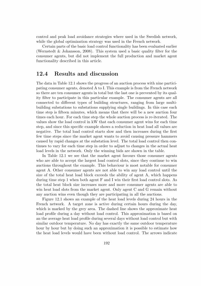
control and peak load avoidance strategies where used in the Swedish network,while the global optimization strategy was used in the French network.

Certain parts of the basic load control functionality has been evaluated earlier(Wernstedt & Johansson, 2008). This system used a basic quality filter for theconsumer agents, but did not implement the full production and market agentfunctionality described in this article.

12.4 Results and discussion

The data in Table 12.1 shows the progress of an auction process with nine partici-pating consumer agents, denoted A to I. This example is from the French networkso there are ten consumer agents in total but the last one is prevented by its qual-ity filter to participate in this particular example. The consumer agents are allconnected to different types of building structures, ranging from large multi-building substations to substations supplying single buildings. In this case eachtime step is fifteen minutes, which means that there will be a new auction fourtimes each hour. For each time step the whole auction process is re-iterated. Thevalues show the load control in kW that each consumer agent wins for each timestep, and since this specific example shows a reduction in heat load all values arenegative. The total load control starts slow and then increases during the firstfew time steps since the market agent wants to avoid causing pressure hammerscaused by rapid changes at the substation level. The total load control then con-tinues to vary for each time step in order to adjust to changes in the actual heatload levels in the network. Only the winning bids are shown in the table.

In Table 12.1 we see that the market agent favours those consumer agentswho are able to accept the largest load control slots, since they continue to winauctions throughout the example. This behaviour is most notable for consumeragent A. Other consumer agents are not able to win any load control until thesize of the total heat load block exceeds the ability of agent A, which happensduring time step 1 when both agent F and I win their first load control slots. Asthe total heat block size increases more and more consumer agents are able towin heat load slots from the market agent. Only agent C and G remain withoutany auction wins even though they are participating in all the auctions.

Figure 12.1 shows an example of the heat load levels during 24 hours in theFrench network. A target zone is active during certain hours during the day,which is marked by the grey area. The dashed line shows the approximate heatload profile during a day without load control. This approximation is based onan the average heat load profile during several days without load control but withsimilar outdoor temperature. No day has exactly the same outdoor temperaturehour by hour but by doing such an approximation it is possible to estimate howthe heat load levels would have been without load control. The arrows indicate

192

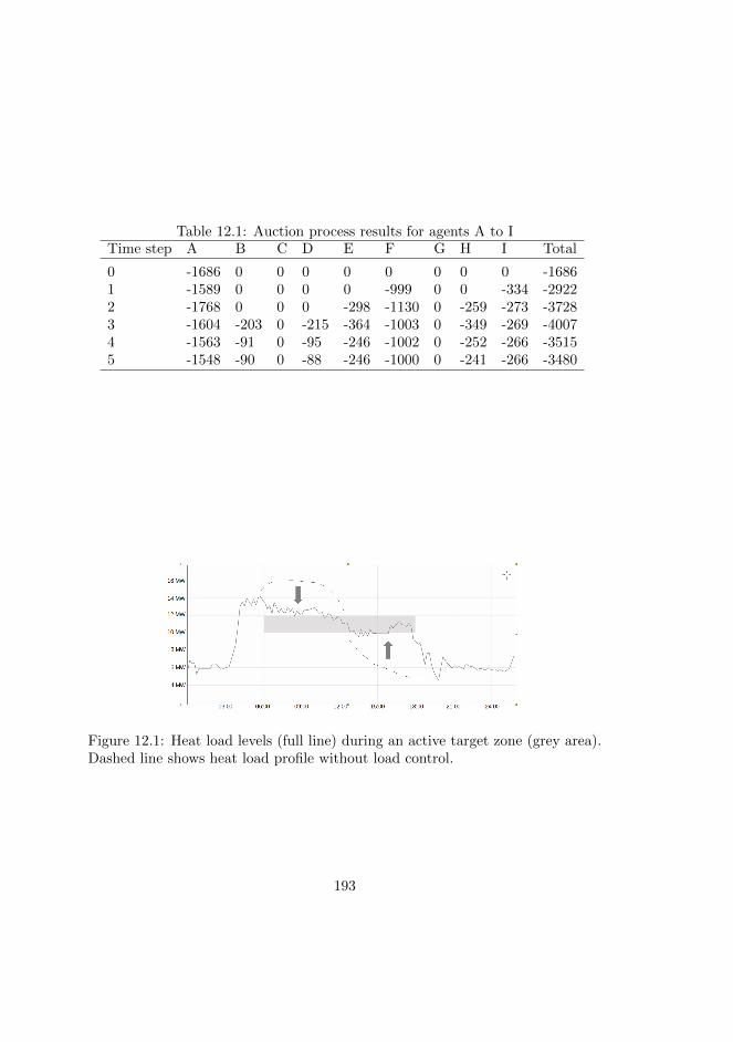
Table 12.1: Auction process results for agents A to ITime step A B C D E F G H I Total

0 -1686 0 0 0 0 0 0 0 0 -16861 -1589 0 0 0 0 -999 0 0 -334 -29222 -1768 0 0 0 -298 -1130 0 -259 -273 -37283 -1604 -203 0 -215 -364 -1003 0 -349 -269 -40074 -1563 -91 0 -95 -246 -1002 0 -252 -266 -35155 -1548 -90 0 -88 -246 -1000 0 -241 -266 -3480

Figure 12.1: Heat load levels (full line) during an active target zone (grey area).Dashed line shows heat load profile without load control.

193

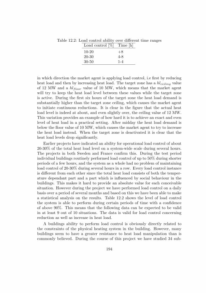
Table 12.2: Load control ability over different time rangesLoad control [%] Time [h]

10-20 +820-30 4-830-50 1-4

in which direction the market agent is applying load control, i.e first by reducingheat load and then by increasing heat load. The target zone has a hlceiling valueof 12 MW and a hlfloor value of 10 MW, which means that the market agentwill try to keep the heat load level between these values while the target zoneis active. During the first six hours of the target zone the heat load demand issubstantially higher than the target zone ceiling, which causes the market agentto initiate continuous reductions. It is clear in the figure that the actual heatload level is indeed at about, and even slightly over, the ceiling value of 12 MW.This variation provides an example of how hard it is to achieve an exact and evenlevel of heat load in a practical setting. After midday the heat load demand isbelow the floor value of 10 MW, which causes the market agent to try to increasethe heat load instead. When the target zone is deactivated it is clear that theheat load levels drop significantly.

Earlier projects have indicated an ability for operational load control of about20-30% of the total heat load level on a system-wide scale during several hours.The projects in both Sweden and France confirm this. During the test periodindividual buildings routinely performed load control of up to 50% during shorterperiods of a few hours, and the system as a whole had no problem of maintainingload control of 20-30% during several hours in a row. Every load control instanceis different from each other since the total heat load consists of both the temper-ature dependant part and a part which is influenced by social behaviour in thebuildings. This makes it hard to provide an absolute value for each conceivablesituation. However during the project we have performed load control on a dailybasis over a period of several months and based on this we have been able to makea statistical analysis on the results. Table 12.2 shows the level of load controlthe system is able to perform during certain periods of time with a confidenceof above 90%. This means that the following data can be expected to be validin at least 9 out of 10 situations. The data is valid for load control concerningreduction as well as increase in heat load.

A buildings ability to perform load control is obviously directly related tothe constraints of the physical heating system in the building. However, manybuildings seem to have a greater resistance to heat load manipulation than iscommonly believed. During the course of this project we have studied 34 sub-

194

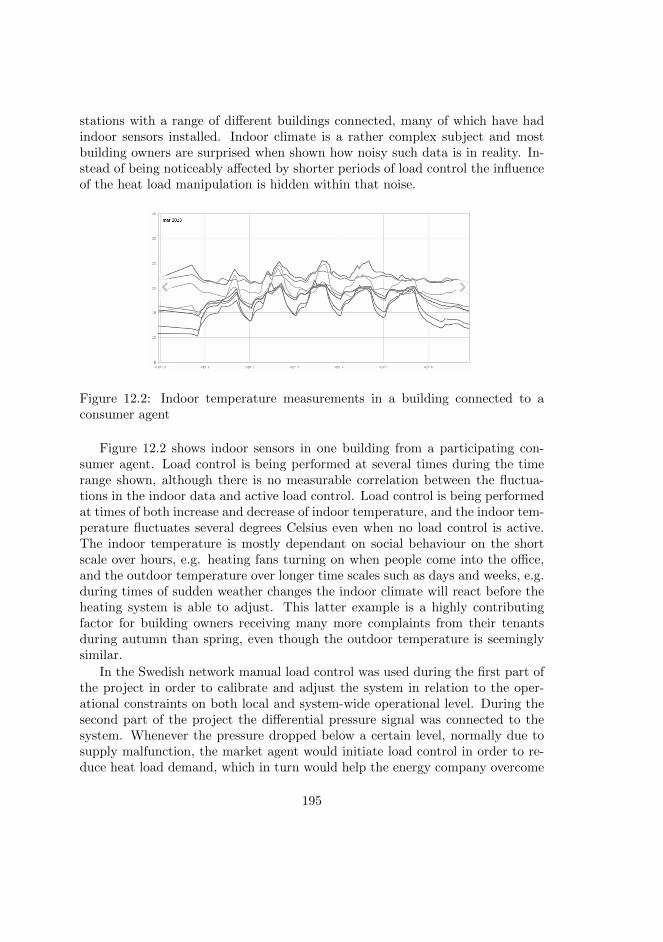
stations with a range of different buildings connected, many of which have hadindoor sensors installed. Indoor climate is a rather complex subject and mostbuilding owners are surprised when shown how noisy such data is in reality. In-stead of being noticeably affected by shorter periods of load control the influenceof the heat load manipulation is hidden within that noise.

Figure 12.2: Indoor temperature measurements in a building connected to aconsumer agent

Figure 12.2 shows indoor sensors in one building from a participating con-sumer agent. Load control is being performed at several times during the timerange shown, although there is no measurable correlation between the fluctua-tions in the indoor data and active load control. Load control is being performedat times of both increase and decrease of indoor temperature, and the indoor tem-perature fluctuates several degrees Celsius even when no load control is active.The indoor temperature is mostly dependant on social behaviour on the shortscale over hours, e.g. heating fans turning on when people come into the office,and the outdoor temperature over longer time scales such as days and weeks, e.g.during times of sudden weather changes the indoor climate will react before theheating system is able to adjust. This latter example is a highly contributingfactor for building owners receiving many more complaints from their tenantsduring autumn than spring, even though the outdoor temperature is seeminglysimilar.

In the Swedish network manual load control was used during the first part ofthe project in order to calibrate and adjust the system in relation to the oper-ational constraints on both local and system-wide operational level. During thesecond part of the project the differential pressure signal was connected to thesystem. Whenever the pressure dropped below a certain level, normally due tosupply malfunction, the market agent would initiate load control in order to re-duce heat load demand, which in turn would help the energy company overcome

195

their supply problems without having to start the peak load boiler. Such tempo-rary malfunctions appeared quite often and during the test period of four monthssuch pressure drops caused the market agent to initiate load control twenty-threetimes. These load control instances varied in size from 0.15 MWh to 17 MWh intotal energy content. The average energy content of a load control instances wasabout 5 MWh. In total these load control instances comprised 100 MWh. Themajority of the load control lasted between 3 to 6 hours. Most of load controlwas initiated during the two coldest months of the test period. In addition to thismanual load control was used on a few single occasions when the energy companyknew that there would be supply problems even before the differential pressuredropped.

12.5 Conclusions

We have presented a working system for demand side management through multi-agent based operational load control. In addition to this we have confirmed earlierresults relating to certain aspects of operational load control in district heatingsystems. The system has been active in two different district heating systemsand the results show the ability of the system to routinely perform operationalload control of 20-30% on a system scale during several hours.

It is shown that a multi-agent architecture for demand side management canbe used to implement different types of operational load control strategies. Wehave presented results relating to three such different strategies; manual load con-trol, peak load avoidance and global system optimization together with heat loadforecasting and optimization. The manual load control and peak load avoidancestrategies are relevant for most district heating systems where peak load boilersare used. The cost of producing energy through peak load boilers is often higherthan the consumer end price, which makes it highly relevant to handle. Thepeak load avoidance strategy is easy to implement since it uses the same controlfeedback system normally used for the peak load boiler itself, in this case thedifferential pressure in the network. The global system optimization strategy issomewhat more complex since it uses heat load forecasting as well as optimizationmodels in order to find future heat load levels, and it normally requires a moreactive and informed operational personnel. The financial incentives to use theglobal optimization strategy is normally found in situations when the companydistributing and selling the energy is not the same as the company generating theheat for the district heating system. Another situation when such more complexsystems are appropriate is when there is third party access in one district heatingsystem, i.e. when different energy companies compete in the same physical arena.This situation is obviously normal in most power grids but it is not as commonin district heating systems.

196

The presented system combines a production agent with a market agent andnumerous consumer agents in order to achieve the desired functionality. Theproducer agent forecasts the heat load and calculates the optimal operationalproduction levels in relation to the forecast. When there is a difference betweenthe actual heat load levels and the requested optimal levels, or if an external signalsuch as a pressure drop triggers, the market agent will distribute load controlamong the consumer agents using an auction mechanism in order to minimizethis difference. The consumer agents implements a quality filter in order to securerequired quality of service while trying to participate in as much load control aspossible. The agent-based architecture of this system ensures a self balancingprocess which can be used for numerous aspects within operational demand sidemanagement.

12.6 Acknowledgments

The authors would like to thank Karlshamn Energi, Dalkia and Veolia Environ-nement Research & Innovation (VERI) for their support and for letting us useoperational data from system installations in Sweden and France, and NODAIntelligent Systems for support regarding server and data access.

This paper was made possible through a grant (Fjarrsynsprojekt 6268) fromthe Swedish District Heating Association.

We dedicate this article to Fredrik Wernstedt.

197

198

Chapter 13

Paper XII - A dynamicsimulation of theproduction, distribution andconsumption of districtheating systems: Averification study of Dhemos

Simulation tools are regularly used for optimizing the operational and strategicfunctionality of district heating systems. Normally, the production, distributionand consumption are modelled separately, but by integrating these models severaladvantages can be achieved, e.g., increased realism. Dhemos is a simulation sys-tem that combines different simulation models in order to achieve a system levelmodel of a district heating system. It has been developed and refined during morethan a decade and has been used within several projects, e.g. in order to supportthe development of new control strategies.

In this paper we describe the verification process of Dhemos and discuss itsvalidation process. The current status and capacity of Dhemos is evaluated andthe functionality of Dhemos compared to a commercial simulation tool availableon the market. The results verify that the computations seem to be correct andindicates that Dhemos is useful for practical applications in real-world settings.Moreover, Dhemos has a number of fundamental design characteristics which

199

suggest potential also for future development. However, it is noticed that Dhemoscurrently lacks important functionality regarding the user interface in comparisonwith commercial alternatives.

13.1 Simulation system overview

Simulation techniques are regularly used in the district heating industry in orderto simulate physical, operational and financial processes relating to production,distribution and consumption. By building theoretical models of the real worldequivalent a process can be studied without having to invest in costly and time-consuming experimentation (Banks et al., 2001). Traditionally, the simulationtools available focus on single distinct issues within the district heating domain,e.g. long term production planning from financial aspects or short term opera-tional analysis regarding pressure head and temperature levels in the distributionnetwork (Arvastson, 2001).

In most available simulation systems for district heating there is a separationbetween tools for production, consumption and distribution. Tools for produc-tion simulation normally focus on the financial aspects of long to medium termplanning, while simulation tools for distribution normally focus on short termplanning in relation to operational behaviour of flow, pressure drops and tem-perature losses with the district heating network. There are not many dedicatedtools for modelling consumption behaviour in district heating systems, althoughsimple versions of such models are possible to implement manually in tools likeMatlab or its equivalence. However, such systems are usually severely limitedin their usability. Most commercially available simulation systems for districtheating either handle long term simulation in production or short term planningin distribution.

13.1.1 The Dhemos simulation framework

Dhemos is an framework for combining simulation models for production, distri-bution and consumption. The basic idea behind Dhemos architecture is that itshould facilitate a more modular approach when combining different simulationmodels. Table 13.1 provides an overview of the framework. For each level of thedifferent module an example of a simulation value relating to that level is shown.Obviously there are many other values on each level, but the example is shownto give an idea of the focus.

The first version of Dhemos was developed in 2002 and implemented a dis-tribution model based on equations compiled and adapted by Pall Valdimarsson(Valdimarsson, 1993). At the time, most distribution models were based on ag-gregation models in which the components of the network are bundled together.

200

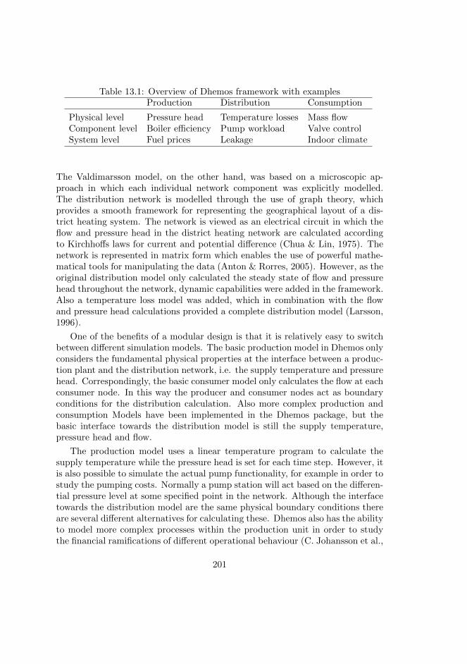
Table 13.1: Overview of Dhemos framework with examplesProduction Distribution Consumption

Physical level Pressure head Temperature losses Mass flowComponent level Boiler efficiency Pump workload Valve controlSystem level Fuel prices Leakage Indoor climate

The Valdimarsson model, on the other hand, was based on a microscopic ap-proach in which each individual network component was explicitly modelled.The distribution network is modelled through the use of graph theory, whichprovides a smooth framework for representing the geographical layout of a dis-trict heating system. The network is viewed as an electrical circuit in which theflow and pressure head in the district heating network are calculated accordingto Kirchhoffs laws for current and potential difference (Chua & Lin, 1975). Thenetwork is represented in matrix form which enables the use of powerful mathe-matical tools for manipulating the data (Anton & Rorres, 2005). However, as theoriginal distribution model only calculated the steady state of flow and pressurehead throughout the network, dynamic capabilities were added in the framework.Also a temperature loss model was added, which in combination with the flowand pressure head calculations provided a complete distribution model (Larsson,1996).

One of the benefits of a modular design is that it is relatively easy to switchbetween different simulation models. The basic production model in Dhemos onlyconsiders the fundamental physical properties at the interface between a produc-tion plant and the distribution network, i.e. the supply temperature and pressurehead. Correspondingly, the basic consumer model only calculates the flow at eachconsumer node. In this way the producer and consumer nodes act as boundaryconditions for the distribution calculation. Also more complex production andconsumption Models have been implemented in the Dhemos package, but thebasic interface towards the distribution model is still the supply temperature,pressure head and flow.

The production model uses a linear temperature program to calculate thesupply temperature while the pressure head is set for each time step. However, itis also possible to simulate the actual pump functionality, for example in order tostudy the pumping costs. Normally a pump station will act based on the differen-tial pressure level at some specified point in the network. Although the interfacetowards the distribution model are the same physical boundary conditions thereare several different alternatives for calculating these. Dhemos also has the abilityto model more complex processes within the production unit in order to studythe financial ramifications of different operational behaviour (C. Johansson et al.,

201

2012a).

The consumption model is used to calculate the flow value for each consumerin the network. These flow values are boundary conditions for the distributionmodel, just as the temperature and pressure head values are production bound-aries. In the basic consumer model the flow is modelled based on the energysignature of the building in relation to the current outdoor temperature and anestimated cooling ability of the heat exchanger at the specific customer model.By combining these values it is possible to estimate a flow value which then actsas a boundary value for the distribution model. In this study the basic model con-sumer model has been used since a predictable behaviour was required in orderto facilitate a comparison with the existing simulation model. However, if a morecomplex behaviour is required it is possible to use an option which separates theconsumer model into two different models, one for the heating system and onefor the tap water usage (Arvastsson & Wollerstrand, 1997). The heating systemconsists of an energy balance model for calculating the indoor temperature and asubstation component which calculates the energy transfer into the building. Thesubstation component uses the outdoor temperature as input when calculatingthe energy usage of the substation, which is the way most district heating substa-tions work in real life. The substation component basically builds a simple modelof an actual heating system starting with the heat exchanger package itself. Thisis modelled as a parallel-coupled substation since this provides a good descriptionof the relations between flow rate and temperature (Arvastson, 2001). Based onthe input from the substation component the energy balance model will calculatethe indoor climate. An energy balance model is based on the fundamental formof energy input minus energy output in order to estimate if the energy contentof the building is stable or deviating in any way.

Two different energy balance models are implemented in Dhemos. The basicversion uses a fundamental formula based on an estimate of the time constantof the building (Osterlind, 1982). In the original form, the time constant iscalculated based on a total loss of heat load input. However, in an operationalsetting this is rarely the case. Therefore the time constant is changed based onthe supplied heat load levels in relation to the building characteristics (Selinder& Zinko, 2003). A more thorough description of this process has been presentedin a previous article (C. Johansson & Wernstedt, 2005).

Dhemos also uses a more complex indoor model in order to describe a moredetailed behaviour relating to small deviations in the heat load supply. Thismodel is based on a system of differential equations which describe the indoortemperature and the average temperature within the building structure. Nor-mally these type of models require a large set of input data relating to physicalcharacteristics of the individual building which makes it hard to use such modelsin practical settings. The model used in Dhemos is based on the same type of

202

equations but has been reformulated in order to avoid the problem with param-eter input. This was done by transforming the physical model into a black boxsimulation model (Cauer, Mathis, & Pauli, 2000). In the black box model onlytwo simulation parameters needs to be set, and they are derived from the timeconstant and energy signature of the building. Finding these values involve usingsuccessive runs of steady state simulations in relation to the time constant andthe energy signature. However, in order to facilitate the use of the model inpractical settings a set of building templates have been developed. By using thetemplates it is easy to estimate usable input values for the simulation based onthe generic size of different building types. The theoretical background of thisblack box model is thoroughly described in a previous paper (C. Johansson etal., 2012b).

The non-temperature dependent part of the heat load is primarily due to tapwater usage. This can be calculated based on a statistical analysis of historicalmeasurement data. Dhemos uses a model based on measurement data relating tobath, wash and kitchen usage of tap water (Holmberg, 1981). Based on this it ispossible to calculate the probability of tap water usage as a function of the timeof day. The tap water usage can also be used as an indicator for social behaviour,i.e. by assuming there is a correlation between how much tap water people useand if they are awake and active.

The Dhemos package uses an event list to handle the input parameters for thedynamic simulation. This list contains events that trigger during the simulation.Each event consist of an identifier, a time stamp and a description string. Theidentifier is predefined value that is connected to different types of input datathat the simulation models use. Examples of this include the outdoor temper-ature or status changes at individual components. The description string cancontain arbitrary data given that the ability to parse the string has been addedto Dhemos. For each simulation time step Dhemos will inspect the event list andcheck if the current time step has any related events, in which case the eventdescription will be parsed as input for simulation step.

Dhemos also contains a pre-processing stage which can be used to populate theevent list. An obvious example of such functionality is if the simulation systemis connected to a weather forecast provider. The event list can also be used forsimulations based on heat load forecasts within the district heating system. Thetotal consumer heat demand is primarily related to the outdoor temperature butit is also influenced by social behaviour, especially when studying data on shorttime frames. If Dhemos is equipped with a heat load forecasting system, theevent list can be used to set actual heat loads throughout the simulation run.This would override the normal simulation process in which the heat demand iscalculated dynamically in relation to the outdoor temperature. The event listcan also be used to evaluate non-standard component specific behaviour such as

203

fault analysis or operational demand side management. The general idea behindthe event list is to be able to introduce behaviour which is not related to thebasic physical equations of each component type.

During the course of this project there has also been some development ofthe core distribution model. The distribution module in Dhemos has two basicequation models, i.e. the special case model and the general model. The specialcase model handles a distribution situation where the supply side of the districtheating network can be modelled as a tree structure. This implies that only oneproduction unit and no storage tanks are allowed in the system. This leaves amodel that is very easy to solve analytically. However, most district heating net-works feature several production units in combination with distribution loops andpossibly storage tanks. For such situations the general model is used. Handlingthis requires using a Newton algorithm for iterating towards an approximate so-lution (Mathews & Fink, 2004). In the latest version of Dhemos a new generaldistribution model was added in order to achieve an increased robustness com-pared to the original model (Hassine & Eicker, 2011). The current model is easierto implement and handle in relation to larger networks which also benefits thescalability of the system.

13.1.2 Implementation of the Dhemos software package

The first version of the Dhemos simulation tool was developed during 2002-2003.The original purpose of the system was to aid in the development of agent-basedsystem optimization tools for district heating systems. In order to do this thesystem needed to combine simulation models relating to production, distributionand consumption into one coherent package. This first version was implementedpurely in Java and featured a graphical user interface for building and maintainingmodels of district heating systems. All the core simulation functionality wasalso developed in Java, including all required mathematical functionality. Asthe project developed it became apparent that this was not an optimal solutiondue to performance issues. In order rectify this situation a new version of thecore simulation tool was developed in C++ which was able to use the Matlabapplication programming interface for matrix handling capabilities. Althoughtechnically sound this solution was in conflict with the aim of developing a freeopen source simulation tool since this set-up required each user of Dhemos toalso have a commercial licence for Matlab. In the current version of Dhemosa transition has been made from Matlab to the Octave framework. Octave isan open source Matlab clone, with much of the original functionality found inMatlab. The current version is developed and run on the Linux operation system,but it can also be compiled and packaged in order to run on Microsoft Windows.

Since the early Java version the file system of Dhemos has changed in order to

204

increase computational efficiency and scalability. Due to this the original graph-ical user interface is no longer compatible with the current version of Dhemos.At the moment a Dhemos session is managed through a text-based terminal, butin the future some form of graphical user interface will be developed in order tofacilitate a greater user base.

Dhemos uses files with comma separated values. This is done in order toease the conversion to spreadsheet tools such as OpenOffice Calc or MicrosoftExcel. The basic input file for Dhemos is the map file which specifies how all thecomponents in the network are connected. The file also contains the individualparameter values for all the components. In addition to this Dhemos also usesa set of different files specifying specific simulation scenario parameters. Thesimulator file contains data relating to the current simulation to be calculated,such as simulation length, time step length, log frequency and choice of calculationmodel. Each calculation model has its own configuration file since the models tendto require quite a diverse set of input parameters. Thus, depending on the choiceof calculation model in the simulation file, a different model configuration file willbe used. The final file that Dhemos uses is the event file which contain the eventlist previously described. The event list can be populated either automaticallyby the pre-processor or manually. Either way, Dhemos requires an event file atleast containing at least the outdoor temperature for the current simulation run.

When Dhemos is started a sub-folder is automatically created in the desig-nated log folder. The sub-folder is named by the system time at the start of thesimulation. This makes it easy to keep track of different simulation runs. Duringthe simulation this folder will be populated by files correlating to the componentsspecified in the district heating network. It is possible to specific what type ofcomponents should log data or not in order to keep the data set more easily man-ageable. A simulation run of a large district heating network can easily generateseveral gigabytes of data with full logging an all components if the simulationhas a long simulation length in relation to the size of the time step.

13.1.3 Related simulation studies

The basic theoretical background for the Dhemos platform has been describedin previous papers (Wernstedt et al., 2003), (C. Johansson & Wernstedt, 2005).In addition to this the functionality of Dhemos has been studied and verified intwo projects funded by the Swedish District Heating Association over the years2010-2012. The first of these projects compared the functionality of Dhemos witha commercially available simulation tool in order to verify the correctness of theoutput of the Dhemos system (C. Johansson & Wernstedt, 2010a). The focus ofthe project was the modelling of the distribution network. In this project, datafrom the Ale network in Gothenburg was used. This network was previously

205

modelled in an existing tool which eased the verification process. The studyconcluded that Dhemos produced correct output when compared to the existingmodel. There were minor differences in the results but it was concluded that thiswas more likely due to differences in network representation and simulation inputrather than any deviation in the actual simulation calculations. The fundamen-tal equation models describing pressure losses, flow and temperature changes inincompressible fluids within piping systems are generally know. However, thereare likely differences in the way the network is represented internally in the simu-lation models and how the the equation models for the different components arecombined. In the study it was concluded that calculations governing the pres-sure loss throughout the piping system were most likely to vary between the twomodels. This is due to the many variables influencing the calculation, such aswater velocity, roughness of pipe walls, approximate methods for calculating thefriction factor and temperature dependent values for the viscosity and density ofthe water.

The second project focused mainly on further development of the productionmodels in the Dhemos package (C. Johansson & Wernstedt, 2012). One of theprimary goals was to handle the foundations of production analysis in relation tofinancial and environmental factors. During the project, production analysis wasbased on a fuel mix of biomass for the base load with oil for peak load produc-tion. However, the Dhemos framework facilitates the addition and manipulationof financial and environmental variables. Additional support for event-driven andalgorithm-based processes was also added during this project, which facilitatesthe process of adding new functionality. The second goal of the project was to de-velop and analyse methods for identifying system wide energy efficiency measuresin smaller district heating networks. In the project the process of configuring andcalibrating Dhemos for a specific district heating system was also further devel-oped, and how by using the event list and algorithm-based functionality additionspotential measures can be identified and dynamically studied. The third goal ofthe project was to describe a method for evaluating the impact of such measuresfrom financial and environmental perspectives. To this end three different energyefficiency schemes were described. The schemes all focused on active demandside management and were based on group coordination, market coordinationand market coordination with predictive capabilities respectively.

During the project the issue of a dedicated graphical user interface has beendiscussed, and interviews with potential users has been performed. One veryapparent conclusion of the interviews was that Dhemos has to be able to run ona stand alone computer with Microsoft Windows in order to get any traction atall among the user base. Another part of the system that was deemed crucial wasthe ability to add functionality for operational production optimization on hourlybasis. Overall the continuous transition from stationary and long-term simulation

206

scenarios to operational management simulation has been a consistent trend inthe Dhemos development effort throughout the years.

13.2 Experimental set-up

This study used data from Gothenburg Energy concerning the district heatingsystem in Ale, a small town close to Gothenburg. The Ale network is part ofthe larger Gothenburg district heating network, although it is geographicallyseparate from Gothenburg. For this network there existed a simulation modelusing commercial simulation software, and data from this system was used asreference for this study. In order to model the Ale network in Dhemos, theavailable component and network layout data were compiled and analysed.

The district heating system in Ale has a general layout like a tree structurestarting in the south at Angered which then moves north for a split betweenKungalv and Heljered. Angered, Eka, Perstorp and Heljered are productionnodes in the network. In Angered the Ale network is connected to the rest ofthe district heating network in Gothenburg. In the simulation model this isconsidered to be the primary production node since most of the heat demand iscovered through this flow.

There exists a range of simulation systems aimed at different aspects of districtheating. In this study the primary goal has been results relating to distributionanalysis.

13.3 Results

Table 13.2 shows the mass flow at different consumer clusters. The values arecalculated by Dhemos and the reference system. All the results relate to a simu-lation scenario with an outdoor temperature of -16◦C.

Table 13.3 shows the pressure loss along the distribution pipes in the system.The pipe D1 is the longest pipe at more than 3.8km which obviously translatesto a higher pressure loss than the other shorter pipe sections.

Table 13.4 shows the pressure head at different production points in the net-work. The pressure head is highest at Angered (P1) where the Ale-networkreceives flow input from the Gothenburg district heating network. From P1 thepressure head drops as the water propagates throughout the network, except inP6 where there is a production unit with a pumping station.

207

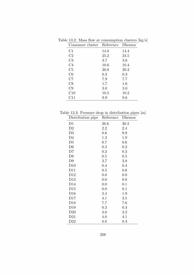
Table 13.2: Mass flow at consumption clusters [kg/s]Consumer cluster Reference Dhemos

C1 14.8 14.4C2 25.2 24.5C3 3.7 3.6C4 10.6 10.4C5 20.8 20.3C6 0.3 0.3C7 7.9 7.7C8 1.7 1.6C9 3.0 3.0C10 10.5 10.2C11 9.9 9.6

Table 13.3: Pressure drop in distribution pipes [m]Distribution pipe Reference Dhemos

D1 26.6 30.3D2 2.2 2.4D3 8.6 9.9D4 1.3 1.9D5 0.7 0.6D6 0.2 0.2D7 0.3 0.3D8 0.5 0.5D9 3.7 3.8D10 0.4 0.4D11 0.5 0.6D12 0.0 0.0D13 0.0 0.0D14 0.0 0.1D15 0.0 0.1D16 2.4 1.9D17 4.1 3.5D18 7.7 7.6D19 0.3 0.3D20 3.0 3.2D21 4.0 4.1D22 8.0 8.3

208

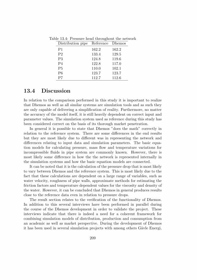
Table 13.4: Pressure head throughout the networkDistribution pipe Reference Dhemos

P1 162.2 162.2P2 133.4 129.5P3 124.8 119.6P4 122.8 117.0P5 110.0 102.1P6 123.7 123.7P7 112.7 112.6

13.4 Discussion

In relation to the comparison performed in this study it is important to realizethat Dhemos as well as all similar systems are simulation tools and as such theyare only capable of delivering a simplification of reality. Furthermore, no matterthe accuracy of the model itself, it is still heavily dependent on correct input andparameter values. The simulation system used as reference during this study hasbeen considered correct on the basis of its thorough market penetration.

In general it is possible to state that Dhemos ”does the math” correctly inrelation to the reference system. There are some differences in the end resultsbut they are most likely due to different was in representing the network anddifferences relating to input data and simulation parameters. The basic equa-tion models for calculating pressure, mass flow and temperature variations forincompressible fluids in pipe system are commonly known. However, there ismost likely some difference in how the the network is represented internally inthe simulation systems and how the basic equation models are connected.

It can be noted that it is the calculation of the pressure drop that is most likelyto vary between Dhemos and the reference system. This is most likely due to thefact that these calculations are dependent on a large range of variables, such aswater velocity, roughness of pipe walls, approximate methods for estimating thefriction factors and temperature dependent values for the viscosity and density ofthe water. However, it can be concluded that Dhemos in general produces resultsclose to the reference data even in relation to pressure drops.

The result section relates to the verification of the functionality of Dhemos.In addition to this several interviews have been performed in parallel duringthe course of the Dhemos development in order to validate the project. Theseinterviews indicate that there is indeed a need for a coherent framework forcombining simulation models of distribution, production and consumption froman academic as well as market perspective. During the development of Dhemosit has been used in several simulation projects with among others Gavle Energi,

209

Goteborg Energi, Swedavia, European Spallation Source (ESS), and KarlshamnEnergi (C. Johansson & Wernstedt, 2010a, 2012, 2005; Wernstedt et al., 2003).

13.5 Conclusions

Dhemos forms a basic foundation for simulating district heating networks. Dur-ing the study the functionality of Dhemos has been verified and shown to becorrect. However, at the moment the system is not mature enough to be used asa replacement for commercial alternatives due to lack of an easy to use graphicaluser interface. The system has a scalable design which provides a frameworkfor further development, especially in relation to simulation studies combiningproduction, distribution and consumption.

When comparing Dhemos to commercial alternatives it should be noted thatmany existing simulation tools primarily are used as tools for consultants workingtogether with district heating companies. In other words they are normally notsold as stand-alone products, but rather in a packaged deal consisting of boththe simulation system itself and consulting hours. However, there is nothing inthe open source license of Dhemos preventing people from using it as a tool insuch a context.

The focus of this paper has been to evaluate simulation models in relation dis-tribution calculations. However, Dhemos also incorporates models for simulatingproduction and consumption behaviour. The ability to combine such models intoone framework is considered to be one of the strong points of Dhemos. This is es-pecially true due to the increased academic interest in research combining marketrelated, societal and technological aspects.

13.6 Acknowledgements

The author would like to thank Goteborg Energi for providing measurement dataand access to the existing simulation system.

210

Bibliography

Anastasi, G., Conti, M., Francesco, M., & Passarella, A. (2008). Energy conser-vation in wireless sensor networks: A survey. In Ad hoc networks (Vol. 7).

Andersen, K., Madsen, H., & Hansen, L. (2000). Modelling the heat dynamicsof a building using stochastic differential equations. Energy and Buildings31 , 13-24.

Andersen, K., & Poulsen, H. (1999). Building integrated heating systems. InProceedings of building simulation (Vol. 1).

Andrepont, J. (2012). Thermal energy storage: Optimizing district heatingsystems in more ways than one. District Energy, First Quarter 2012 .

Anton, H., & Rorres, C. (2005). Elementary linear algebra (9th ed.). John Wileyand Sons, Inc.

Arvastson, L. (2001). Stochastic modeling and operational optimization in districtheating systems. Lund Institute of Technology.

Arvastsson, L., & Wollerstrand, J. (1997). On sizing of domestic hot waterheaters of instantaneous type. In Proceedings of of the 6th internationalsymposium on automation of district heating systems.

Aune, M. (2001). Energy technology and everyday life the domestication of eboxin norwegian households. In Proceedings of eceee summer study.

Banks, J., Carson, J., Nelson, B., & Nicol, D. (2001). Discrete-event systemsimulation. Prentice Hall.

Barley, C., Torcellini, P., & Van Geet, O. (2004). The van geet off-grid home: Anintegrated approach to energy savings. National Renewable Energy Labo-ratory.

Bederson, B., & Schneiderman, B. (2003). Information visualization: Readingsand reflections. Morgan Kaufman.

Bjorsell, N. (n.d.). Control strategies for heating systems. University-College ofGavle-Sandviken.

Bohm, B., Lucht, M., Park, Y., Sipila, K., Ha, S., Bong-kyun, K., . . . Wistbacka,M. (2002). Simple models for operational optimisation. NOVEM Report2002:S1 .

211

Box, G., & G.M., J. (1991). Time series analysis. Prentice Hall.Braeutigam, R. (2010). Microeconomics (4th ed.). Wiley.Braun, J. (2003). Load control using building thermal mass. Journal of solar

energy engineering , 125 , 292–301.Cauer, E., Mathis, W., & Pauli, R. (2000). Life and work of wilhelm cauer (1900-

1945). In In proceedings of the 14th international symposium of mathemat-ical theory and systems.

C.E., L., & G.L., V. (1984). Hierarchical economic dispatch for piecewisequadratic cost functions. In Trans power apparatus systems (Vol. 103-6,pp. 1170–1175). The Institute of Electrical and Electronics Engineers, Inc.

Chahwane, L., Stephan, L., Wurtz, E., & Zuber, B. (2011). On a novel approachto control natural and mechanical night ventilation. In In proceedings ofbuilding simulations. 12th conference of international building performancesimulation association. Sydney, Australia.

Chramcov, B., Dostal, P., & Balate, J. (2009). Forecast model of heat demand.In In proceedings of the 28th international symposium on forecasting. HongKong, China.

Chua, L., & Lin, P. (1975). Computer-aided analysis of electric circuits. PrenticeHall.

Clearwater, S. (1996). Market-based control: A paradigm for distributed resourceallocation. World Scientific Publishing Company.

Concrete for energy efficient buildings the benefits of thermal mass. (2007). IrishConcrete Federation Ltd.

Constinescu, N. (2007). District heating and cooling: Country by country, 2007survey. Euroheat and Power.

Dash, R., Rogers, A., S., R., Roberts, S., & Jennings, N. R. (2005). Constrainedbandwidth allocation in multi-sensor information fusion: A mechanism de-sign approach. In Proceedings of the eight international conference on in-formation fusion. Philadelphia, PA, USA.

Dhemos. (2012). http://www.dhemos.org. ([Online; accessed 23-January-2012])Dotzauer, E. (2002). Simple model for prediction of loads in district-heating

systems. Applied Energy , 73 (3–4), 277–284.Dotzauer, E., & Lundh, A. (2004). An application of mixed integer programming

in short-term planning of district cooling. In Proceedings from the 9thinternational symposium on district heating and cooling. Espoo, Finland.

Drysdale, A., & Stang, J. (2002). Optimised dh systems using remote heatmeter communication and control. In Proceedings of the 8th internationalsymposium on district heating and cooling. Trondheim, Norway.

Dutta, P. S., Goldman, C., & Jennings, N. R. (2007). Communicating effectivelyin resource-constrained multi-agent systems. In Proceedings of the 20thinternational joint conference on ai (ijcai). Hyderabad, India.

212

Energimyndigheten. (2002). Flexibiliteten p elmarknadens efterfragesida - hurkan potentialen hos sma elanvandare aktiveras? Author.

Energy in sweden: Facts and figures. (2004). Energimyndighetens Forlag.Fjarrvarme pa varmemarknaden. (2003). Regeringskansliet, Dir 2002:160.Fredriksen, S., & Werner, S. (1993). Fjarrvarme - teori, teknik och funktion.

Studentlitteratur.Fredriksen, S., & Werner, S. (2013). District heating and cooling. Studentlitter-

atur.Fruergaard, T., Christensen, T., & Astrup, T. (2010). Energy recovery from

waste incineration: assessing the importance of district heating networks.Waste Management , 30 (7), 1264-1272.

Gieseler, J., U.D, Heidt, F., & Bier, W. (2003). Combined thermal measurementand simulation for the detailed analysis of four occupied low-energy build-ings. In Proceedings of the 8th ibpsa conference. Eindhoven, Netherlands.

Goldman, C. V., & Zilberstein, S. (2003). Optimizing information exchange incooperative multi-agent systems. In Proceedings of second internationalconference on autonomous agents and multiagent systems (aamas) (pp.137–144).

Grosswindhager, S., Voigt, A., & Kozek, M. (2011). Short-term forecast of systemheat load in district heating networks. In Proceedings of 31th internationalsymposium on forecasting. Prag, Czech Republic.

Gustafsson, J. (2011). Wireless sensor network architectures as a foundation forefficient district heating. Lulea University of Technology.

Hassine, I., & Eicker, U. (2011). Simulation and optimization of the district heat-ing system in scharnhauser park. In Proceedings of 2nd european conferenceon polygeneration. Tarragona, Spain.

Heating, I. D., & Cooling. (2002). Optimised district heating systems usingremote heat meter communication and control. Annex VI report .

Hevner, A., & Chatterjee, S. (2012). Design research in information systems -theory and practice (2010 edition). Springer-Verlag New York Inc.

Hietmaki, T., Kuoppala, J., Kalema, T., & Taivalantti, K. (2003). Thermalmass of buildings central researches and their results. In Tampere univer-sity of technology, institute of energy and process engineering. report 174.Tampere, Finland.

Holmberg, S. (1981). Norrkopingsprojektet - en detaljerad pilotundersokning avhushallens vattenforbrukning (Tech. Rep. No. M81:5). Stockholm, Sweden:Royal Institute of Technology.

Horlock, J. (2008). Combined heat and power, 2th ed. Pergamon Books Inc.Isfalt, E., & Broms, G. (1992). Effekt- och energibesparing genom forenklad

styrning och drift av installationssystem i byggnader (Tech. Rep. Nos.ISRN KTH/IT/M–22–E). Institutionen for Installationsteknik. Kungliga

213

Tekniska Hogskolan.Jacobson, R. e. (1999). Information design. MIT Press.Jayasima, D. N. (1996). Fault tolerance in multisensor networks. IEEE Trans-

actions on Reliability , 45 (2), 308–315.Jennings, N., Corera, J., Laresgoiti, Y., Mamdani, E., Perriollat, F., Sakrek, P.,

& Varga, L. (1996). Using archon to develop real-world dai applicationsfor electricity transportation management and particle accelerator control.In Ieee expert special issue on real world applications of dai systems.

Jensen, L. (1983). Nattsankning av temperatur i flerbostadshus (Tech. Rep. No.R64:1983). Byggforskningsrdet.

Johansson, & Ejeklint. (1991). Laststyrning av direktverkande villor i boden.Uppdrag 2000 .

Johansson, A. (2005). Fault detection of hourly measurements in district heatand electricity consumption. Linkoping University.

Johansson, C. (2010). Towards intelligent district heating. Blekinge Institute ofTechnology. (Licentiate thesis)

Johansson, C., & Wernstedt, F. (2005). Dynamic simluation of district heat-ing systems. In Proceedings of the 1st european simulation and modellingconference. Porto, Portugal.

Johansson, C., & Wernstedt, F. (2010a). Dynamisk fjarrvarmesimulering (Tech.Rep. No. Rapport 2010:1). Svensk Fjarrvarme.

Johansson, C., & Wernstedt, F. (2010b). Heat load reductions and their effect onenergy consumption. In Proceedings of the 12th international symposiumon district heating and cooling. Tallinn, Estonia.

Johansson, C., & Wernstedt, F. (2012). Dynamisk fjarrvarmesimulering i prak-tiken (Tech. Rep. No. Rapport 2012:1). Svensk Fjarrvarme.

Johansson, C., Wernstedt, F., & Davidsson, P. (2010a). A case study on availabil-ity of sensor data in agent cooperation. Computer Science and InformationSystems, 7 (3).

Johansson, C., Wernstedt, F., & Davidsson, P. (2010b). Deployment of agentbased load control in district heating systems. In First international work-shop on agent technologies for energy systems. Toronto, Canada.

Johansson, C., Wernstedt, F., & Davidsson, P. (2012a). Combined heat andpower generation using smart heat grid. In Proceedings of the 4th interna-tional conference on applied energy. Suzhou, China.

Johansson, C., Wernstedt, F., & Davidsson, P. (2012b). Smart heat grid on anintraday power market. In Proceedings of the 3rd agent technology for en-ergy systems workshop at the 11th international conference on autonomousagents and multiagent systems. Valencia, Spain.

Johansson, P. (2003). Laststyrning i smahus - fallstudie hos skanska energi ab.(LUTMDN/TMHP-03/5025-SE)

214

Jonsson, G. (2002). A model for predicting the yearly load in district heatingsystems. In Proceedings of the institution of mechanical engineers, part a:Journal of power and energy 216.

Kato, K., Sakawa, M., Ishimaru, K., Ushiro, S., & Shibano, T. (2008). Heat loadprediction through recurrent neural network in district heating and coolingsystems. In Proceedings of the ieee international conference on systems,man and cybernetics.

Koay, C. A., Lai, L. L., Lee, K., Lu, H., Park, J. B., Song, Y. H., . . . Yu, I. K.(2008). Applications to power system scheduling. In K. Y. Lee & M. A. El-Sharkawi (Eds.), Modern heuristic optimization techniques. The Instituteof Electrical and Electronics Engineers, Inc.

KJ, A., & T, H. (1995). Pid controllers: Theory, design and tuning. InstrumentSociety of America.

Larsson, G. (1996). Dynamik i fjarrvarmesystem (on dynamics in district heatingsystems). Chalmers University of Technology.

Lesser, V., Ortiz, C., & Tambe, M. (2003). Distributed sensor networks: amultiagent perspective. Kluwer Publishing.

Levin, P., & Wesslen, M. (1993). Laststyrning i smahus med vattenburen elvarme.Vattenfall Energimarknad .

Lindkvist, H., Selinder, P., & Wallentun, H. (2005). Utveckling av analysmeto-den felidentifiering i fjarrvarmecentraler med flygfotobilder (Tech. Rep. No.FOU 2005:138). Svensk Fjarrvarme.

Lindkvist, H., & Wallentun, H. (2004). Utvardering av nio fjarrvarmecentraler islagsta (Tech. Rep. No. ZW 04/05). ZW Energiteknik.

Lipaedge. (2005, August). Retrieved fromhttp://www.lipower.org/cei/lipaedge.html

Mathews, J., & Fink, D. (2004). Numerical methods using matlab, (4 ed). Pear-son.

Mazza, R. (2009). Introduction to information visualization. Springer-VerlagLondon Limited.

Morris, F., Braun, J., & Treado, S. (1994). Experimental and simulated perfor-mance of optimal control of building thermal storage. In Ashrae transac-tions.

Newsham, G., & Bowker, B. (2010). The effect of utility time-varying pricingand load control strategies on residential summer peak electricity use: areview. Energy policy , 38 , 3289-3296.

Nielsen, H., & Madsen, H. (2006). Modelling the heat consumption in districtheating systems using a grey-box approach. Energy and Buildings, 38 ,63–71.

Nielson, G., Hagen, H., & Muller, H. (1997). Scientific visualization: Overviews,methodologies and techniques. IEEE Computer Society.

215

Norberg, C. (1990). Direktverkande elradiatorers reglering och konstruktion(Tech. Rep. No. Rapport nr F-90:5). Vattenfall Utveckling AB.

NordPoolSpot. (2012). http://www.nordpoolspot.com. ([Online; accessed 21-January-2012])

Nordvik, H., & Lund, P. E. (2003). How to achieve energy efficient actions as analternative to grid reinforcement. In Proceedings of eceee summer study.

Noren, C., & Pyrko, J. (1998). Laststyrning i lokaler - datorsimulering. LundsTekniska Hogskola.

Olsson Ingvarsson, L., & Werner, S. (2008). Building mass used as short termheat storage. In Proceedings of the 11th international symposium on districtheating and cooling. Reykjavik, Iceland.

Osterlind, B. (1982). Effektbegransning av fjarrvarme (Vol. 63:1982). Byggforskn-ingsradet.

Osterlind, B. (1990). Avlasnings- och kontrollsystem fr fjarrvarmenat (Vol.85:1990). Byggforskningsradet.

Osterman, E. (2005). Remissyttrande over statens energimyndighets rapport:Manadsvis avlasning av elmatare (Vol. 85:1990). Villaagarnas riksforbund.

Pakanen, J., Hyvarinen, J., Kuismin, J., & Ahonen, M. (1996). Fault diagno-sis methods for district heating substations (Tech. Rep.). VTT BuildingTechnology.

Parunak, H. (1998). What can agents do in industry and why? – an overview ofindustrially-oriented r&d at cec.

Persson, M. (2000). Calculation of heat transfer - numerical differential methodsadopted to facilitate use by engineers. Chalmers University of Technology.

Persson, T. (2005). District heating for residential areas with single-family hous-ing. Lund University.

Pyrko, J., Sernhed, H., & J., A. (2005). Hushallen klarar avstangd el. InEnergivarlden 1:2005. Energimyndigheten.

Raberger, L., & Wallentun, H. (1996). Effektivisinger av konventionellafjarrvarmecentraler (Tech. Rep. No. FOU 1996:5). Fjarrvarmeforeningen.

Rade, L., & Westergren, B. (2004). Handbook for science and engineering. 5thed. Studentlitteratur.

Rodgers, J., & Nicewander, W. (1988). Thirteen ways to look at the correlationcoefficient. The American Statistician, 59–66.

Rogers, A., Maleki, S., Ghosh, S., & Jennings, N. R. (2011). Adaptive home heat-ing control through gaussian processprediction and mathematical program-ming. In Second international workshop on agent technologies for energysystems. Taipei, Taiwan.

Rolfsman, B. (2003). Combined heat and power plants and district heating in ade-regulated electricity market. Applied Energy , 78 , 37-52.

Rossing, O., & Johnsson, J. (2005). Samverkande produktions- och distribu-

216

tionsanalys i fjarrvarmesystem (Tech. Rep. No. ISSN 1401-9264). SvenskFjarrvarme.

Rousseeuw, P., & Leroy, A. (2003). Robust regression and outlier detection.Wiley.

Russel, S., & Norvig, P. (1995). Artificial intelligence - a modern approach.Prentice Hall.

Ruud, R. (2009). Energimyndighetens program fr passivhus och lagenergihus(Tech. Rep. No. Remissversion 2009-03-10). Forum fr Energieffektiva byg-gnader.

Selinder, P. (2005). Reducering av anslutningseffekten med hjalp av vv-prioritering. In Fou 2005:141. Svensk Fjarrvarme.

Selinder, P., & Wallentun, H. (2002). Felidentifiering i fc med ”flygfoton” (Tech.Rep. No. FOU 2002:70). Svensk Fjarrvarme.

Selinder, P., & Zinko, H. (2003). Marginaler i fjarrvarmesystem. In Fou 2003:85.Svensk Fjarrvarme.

Shen, J., Lesser, V., & Carver, N. (2003). Minimizing communication cost ina distributed bayesian network using a decentralised mdp. In Proceedingsof second international conference on autonomous agents and multiagentsystems (aamas) (p. 678-685).

Sipila, K., & Karkkainen, S. (2000). Demand side management in district heatingsystems. In Fernwrme international (Vol. 3, pp. 36–45). Euroheat & Power.

Skoog, J. (2005). Pm avseende komfort (Tech. Rep.). AF-Infrastruktur AB.Statistik 2003. (2003). Svensk Fjarrvarme.Taylor, J. (1997). An introduction to error analysis. 2nd ed. University Science

Books.Torriti, J. (2012). Demand side management for the european supergrid. Energy

policy , 44 , 199–206.Valdimarsson, P. (1993). Modelling of geothermal district heating systems. Uni-

versity of Iceland.Wallentun, H. (1999). Effektivisinger av fjarrvarmecentraler - metodik, nyckeltal

och anvandning av driftovervakningssystem (Tech. Rep. No. FOU 1999:27).Fjarrvarmeforeningen.

Wechsler, G. (1944). The measurement of adult intelligence. Baltimore: Williamsand Wilkins.

Weiss, G. e. (2000a). Multiagent systems - a modern approach to distributedartificial intelligence. The MIT Press.

Weiss, G. e. (2000b). Multiagent systems - a modern approach to distributedartificial intelligence. The MIT Press.

Wernstedt, F. (2005). Multi-agent systems for district heating management.Blekinge Institute of Technology. (Doctoral thesis)

Wernstedt, F., Davidsson, P., & Johansson, C. (2003). Simulation of district

217

heating systems for evaluation of real-time control strategies. In Proceedingsof the 1st european simulation and modelling conference.

Wernstedt, F., Davidsson, P., & Johansson, C. (2007). Demand side managementin district heating systems. In Proceedings of sixth international conferenceon autonomous agents and multiagent systems (aamas). Honolulu, Hawaii,USA.

Wernstedt, F., & Johansson, C. (2008). Intelligent distributed load control. InProceedings of the 11th international symposium on district heating andcooling. Reykjavik, Iceland.

Wernstedt, F., & Johansson, C. (2009). Demonstrationsprojekt inom effekt ochlaststyrning (Tech. Rep. No. ISBN 978-91-7381-041-8). Svensk Fjarrvarme.

Wernstedt, F., Johansson, C., & Wollerstrand, J. (2008). Sankning av returtem-peraturer genom laststyrning. In Fou 2008:2. Svensk Fjarrvarme.

Wigbels, M., Bohm, B., & Sipilae, K. (2005). Dynamic heat storage optimizationand demand side management. In Annex vii i 2005:8dhc-05.06. Interna-tional Energy Agency.

Wooldridge, M. (2002). Introduction to multiagent systems. John Wiley andSons.

Xu, P., Haves, P., Piette, M., & Zagreus, L. (2006). Demand shifting with thermalmass in large commercial buildings: Field tests, simulations and audits(Tech. Rep. No. Pier Final Project Report). California Energy Commission.

Ygge, F., & Akkermans, H. (1999). Decentralized markets versus central control:A comparative study. Journal of Artificial Intelligent Research (JAIR), 11 ,301-333.

Ygge, F., & Akkermans, J. (1996). Power load management as a computationalmarket. In Proceedings of the second international conference on multi-agent systems (icmas) (p. 393-400).

Yliniemi, K. (2005). Fault detection in district heating substations (Tech. Rep.No. 2005:60). Lulea University of Technology.

218

ON INTELLIGENT DISTRICT HEATING

ON

INT

EL

LIG

EN

T D

IST

RIC

T H

EA

TIN

G

Christian Johansson

Christian Johansson

Blekinge Institute of Technology

Doctoral Dissertation Series No. 2014:07

Department of Computer Science and Engineering 2014:07

ISSN: 1653-2090

ISBN: 978-91-7295-280-5

ABSTRACTIntelligent district heating is the combination of traditional district heating engineering and mo-dern information and communication technology. A district heating system is a highly complex environment consisting of a large number of distributed entities, and this complexity and geo-graphically dispersed layout suggest that they are suitable for distributed optimization and mana-gement. However, this would in practice imply a transition from the classical production-centric perspective normally found within district heating management to a more consumer-centric per-spective.

This thesis describes a multiagent-based system which combines production, consumption and distribution aspects into a single coherent opera-tional management framework. The flexibility and robustness of the solution in industrial settings is thoroughly examined and its performance is shown to lead to significant operational, financial and environmental benefits compared to current management schemes.

2014:07