numerical solution of boundary layer...v originality report certificate it is certified that phd...
TRANSCRIPT


NUMERICAL SOLUTION OF BOUNDARY LAYER
EQUATION FOR NON-NEWTONIAN FLUID FLOW
A Thesis submitted to Gujarat Technological University
for the Award of
Doctor of Philosophy
in
Science–Maths
By
PATEL JAYSHRIBEN RAMJIBHAI
Enrollment No.: 139997673017
under the supervision of
Prof. (Dr.) MANISHA P. PATEL
GUJARAT TECHNOLOGICAL UNIVERSITY
AHMEDABAD
JUNE 2019

I
@JAYSHRIBEN RAMJIBHAI PATEL

II
DECLARATION
I declare that the thesis entitled “NUMERICAL SOLUTION OF BOUNDARY LAYER
EQUATION FOR NON-NEWTONIAN FLUID FLOW’’ submitted by me for the
degree of Doctor of Philosophy is the record of research work carried out by me during the
period from February 2014 to June 2019 under the supervision of Prof.(Dr.)
MANISHA P. PATEL, Assistant Professor in Mathematics, Sarvajanik College of
Engineering and Technology, Surat and this has not formed the basis for the award of any
degree, diploma, associateship, fellowship, titles in this or any other University or other
institution of higher learning.
I further declare that the material obtained from other sources has been duly acknowledged
in the thesis. I shall be solely responsible for any plagiarism or other irregularities, if
noticed in the thesis.
Signature of the Research Scholar: Date: 26/06/2019
Name of Research Scholar: Patel Jayshriben Ramjibhai
Place: Unjha

III
CERTIFICATE
I certify that the work incorporated in the thesis “NUMERICAL SOLUTION OF
BOUNDARY LAYER EQUATION FOR NON-NEWTONIAN FLUID
FLOW’’submitted by PATEL JAYSHRIBEN RAMJIBHAI was carried out by the
candidate under my supervision/guidance. To the best of my knowledge: (i) the candidate
has not submitted the same research work to any other institution for any degree/diploma,
Associateship, Fellowship or other similar titles (ii) the thesis submitted is a record of
original research work done by the Research Scholar during the period of study under my
supervision, and (iii) the thesis represents independent research work on the part of the
Research Scholar.
Signature of Supervisor: Date: 26/06/2019
Name of Supervisor: Prof. (Dr.) MANISHA P. PATEL
Place: Surat

IV
Course-work Completion Certificate
This is to certify that PATEL JAYSHRIBEN RAMJIBHAI, Enrollment no.
139997673017 is a PhD scholar enrolled for PhD program in the branch Science-Maths of
Gujarat Technological University, Ahmedabad.
(Please tick the relevant option(s))
She has been exempted from the course-work (successfully completed during
M.Phil Course).
She has been exempted from Research Methodology Course only
(successfully completed during M.Phil Course).
She has successfully completed the PhD course work for the partial
requirement for the award of PhD Degree. His/ Her performance in the course work
is as follows:
Grade Obtained in Research Methodology
(PH001)
Grade Obtained in Self Study Course
(Core Subject)
(PH002)
CC BB
Signature of Supervisor:
Name of Supervisor: Prof. (Dr.) MANISHA P. PATEL
√

V
Originality Report Certificate
It is certified that PhD Thesis titled “NUMERICAL SOLUTION OF BOUNDARY
LAYER EQUATION FOR NON-NEWTONIAN FLUID FLOW’’ by PATEL
JAYSHRIBEN RAMJIBHAI has been examined by us. We undertake the following:
a. Thesis has significant new work / knowledge as compared already published or are
under consideration to be published elsewhere. No sentence, equation, diagram,
table, paragraph or section has been copied verbatim from previous work unless it is
placed under quotation marks and duly referenced.
b. The work presented is original and own work of the author (i.e. there is no
plagiarism). No ideas, processes, results or words of others have been presented as
Author own work.
c. There is no fabrication of data or results which have been compiled/ analysed.
d. There is no falsification by manipulating research materials, equipment or
processes, or changing or omitting data or results such that the research is not
accurately represented in the research record.
e. The thesis has been checked using < name of any reputed plagiarism check
software > (copy of originality report attached) and found within limits as per
GTU Plagiarism Policy and instructions issued from time to time (i.e. permitted
similarity index <=25%).
Signature of the Research Scholar: Date: 26/06/2019
Name of Research Scholar: PATEL JAYSHRIBEN RAMJIBHAI
Place : Unjha
Signature of Supervisor: Date: 26/06/2019
Name of Supervisor: Prof. (Dr.) MANISHA P. PATEL
Place: Surat

VI

VII
PhD THESIS Non-Exclusive License to
GUJARAT TECHNOLOGICAL UNIVERSITY
In consideration of being a PhD Research Scholar at GTU and in the interests of the
facilitation of research at GTU and elsewhere, I PATEL JAYSHRIBEN RAMJIBHAI
having Enrollment no. 139997673017 hereby grant a non-exclusive, royalty free and
perpetual license to GTU on the following terms:
a) GTU is permitted to archive, reproduce and distribute my thesis, in whole or in part,
and/or my abstract, in whole or in part ( referred to collectively as the “Work”)
anywhere in the world, for non-commercial purposes, in all forms of media;
b) GTU is permitted to authorize, sub-lease, sub-contract or procure any of the acts
mentioned in paragraph (a);
c) GTU is authorized to submit the Work at any National / International Library, under
the authority of their “Thesis Non Exclusive License”;
d) The Universal Copyright Notice (©) shall appear on all copies made under the
authority of this license;
e) I undertake to submit my thesis, through my University, to any Library and
Archives. Any abstract submitted with the thesis will be considered to form part
of the thesis.
f) I represent that my thesis is my original work, does not infringe any rights of others,
including privacy rights, and that I have the right to make the grant conferred by this
non-exclusive license.
g) If third party copyrighted material was included in my thesis for which, under the
terms of the Copyright Act, written permission from the copyright owners is
required, I have obtained such permission from the copyright owners to do the acts
mentioned in paragraph (a) above for the full term of copyright protection.
h) I retain copyright ownership and moral rights in my thesis, and may deal with the
copyright in my thesis, in any way consistent with rights granted by me to my
University in this non-exclusive license.
i) I further promise to inform any person to whom I may hereafter assign or license
my copyright in my thesis of the rights granted by me to my University in this non-
exclusive license.

VIII
j) I am aware of and agree to accept the conditions and regulations of PhD including
all policy matters related to authorship and plagiarism.
Signature of the Research Scholar:
Name of Research Scholar: PATEL JAYSHRIBEN RAMJIBHAI
Date: 26/06/2019 Place: Unjha
Signature of Supervisor:
Name of Supervisor: Prof. (Dr.) MANISHA P. PATEL
Date: 26/06/2019 Place: Surat
Seal:
IX
Thesis Approval Form
The viva-voce of the PhD Thesis submitted by .PATEL JAYSHRIBEN RAMJIBHAI
(Enrollment no. 139997673017) entitled “NUMERICAL SOLUTION OF BOUNDARY
LAYER EQUATION FOR NON-NEWTONIAN FLUID FLOW’’ was conducted on
_______________ at Gujarat Technological University.
(Please tick any one of the following option)
The performance of the candidate was satisfactory. We recommend that he/she be
awarded the PhD degree.
Any further modifications in research work recommended by the panel after 3
months from the date of first viva-voce upon request of the Supervisor or request of
Independent Research Scholar after which viva-voce can be re-conducted by the
same panel again.
(Briefly specify the modifications suggested by the panel)
The performance of the candidate was unsatisfactory. We recommend that he/she
should not be awarded the PhD degree.
(The panel must give justifications for rejecting the research work)
----------------------------------------------------- ------------------------------------------------- Name and Signature of Supervisor with Seal 1) (External Examiner 1) Name and Signature
-------------------------------------------------------- ----------------------------------------------------- 2) (External Examiner 2) Name and Signature 3) (External Examiner 3) Name and Signature

X
ABSTRACT
The complex rehology of biological fluids has motivated investigations involving different
non-Newtonian fluids. In recent years, non-Newtonian fluids have become more and more
important industrially. Academic curiosity and practical applications have generated
considerable interest in finding the solutions of differential equations governing the motion of
non-Newtonian fluids. The governing equations of such non-Newtonian fluids are highly non
linear partial differential equations. These fluids flow problems present some interesting
challenges to researchers in engineering, applied mathematics and computer science.
Two dimensional Magneto Hydro Dynamic (MHD) and non-MHD laminar boundary layer
flow of non-Newtonian fluid is analyzed in the present work. Three non-Newtonian fluid
models for the stress-strain relationship Sisko fluid model, Prandtl fluid model and
Williamson fluid model are considered for the different flow geometry (semi-infinite flat plate
& semi infinite moving plate). Governing non linear partial differential equations (PDE) are
transformed into non linear ordinary differential equations (ODE) using group theoretical
methods. The quasi linearization method is then applied to convert the non linear ODE into
linear ODE. The numerical solutions of the resulting linear ordinary differential equations are
obtained using Finite difference method (method carried out with Microsoft excel and
MATLAB coding). The graphical presentation of the velocity profile is given for each
problem.
Calculations on non-Newtonian media present a new challenge in flow analysis. Simulating
these types of flows in order to calculate pipe and pump sizes presents a significant challenge
to the engineer. The stress-strain relationship for different type of viscous-inelastic fluids and
similarity equations using these relationships will be helpful to many researchers and
engineers for further research.
Our aim is to modify similarity techniques and apply it to find similarity solutions of MHD
and non-MHD boundary layer flows of non-Newtonian fluids. Applications of these

XI
techniques are useful for the treatment of engineering boundary value problems. Our aim is to
propose quite a new idea in the theory of similarity analysis and that is approximate similarity
technique. We hope that our proposed approximate similarity technique will be useful to treat
the non-linear partial differential equations.
Scopes of the new proposed technique are wide. It will be useful to solve non-similarity
equations and also hope to derive some closed form solutions. It may be used for finding the
exact solutions for defined fluid models.

XII
Acknowledgement
I am grateful to receive valuable help and encouragement from several persons in course of
this research.
Foremost, I would like to express my sincere thanks to my research supervisor Prof. (Dr.)
Manisha P. Patel, Assistant Professor in Mathematics at Sarvajanik College of Engineering
and Technology (SCET), Surat, for her continuous support during my research work. Her deep
insight and ever-growing knowledge have contributed a great deal in my approach to the
subject. Her guidance, motivation and enthusiasm have striven to make this research work
possible. I feel short of words to express my gratitude towards her.
Besides I would like to thanks the Doctoral Progress Committee (DPC) Members of my
research work, Dr. Mitesh S. Joshi, Associate Professor in Mathematics at C. K. Pithawala
College of Engineering and Technology (CKPCET), Surat and Dr. Hema Surati, Assistant
Professor in Mathematics at Sarvajanik College of Engineering and Technology (SCET), Surat
for their encouragement, insightful comments and excellent suggestions. Also, I would like to
give my special thanks to Dr. M. G. Timol, Professor and In charge Head of the Department in
Mathematics at Veer Narmad South Gujarat University (VNSGU), Surat for his valuable
suggestions.
Words cannot express how grateful to my mother, father, mother-in-law, father-in-law, brother
and sisters for all of the sacrifices that you’ve made on my behalf. Your prayer for me has
sustained me thus far. I am very much thankful to my husband, Dr. Vipul Patel for his
inspiration and confidence in my ability. Without his patience and support, this work would
not have been possible. I feel short of words to express my gratitude towards him. I would also
like to thank my beloved daughter Dhani for her moral and emotional support and for always
cheering me up.
I am also grateful to my family members, friends and colleagues who have directly or
indirectly supported me along the way.
JAYSHRI PATEL

XIII

XIII
Table of Content
1. Copyright……………………………………………………………………..... I
2. Declaration…………………………………………………………………….. II
3. Certificate by the Supervisor…………………………………………………... III
4. Coursework Completion Certificate…………………………………………… IV
5. Originality Certificate…………………………………………………………. V
6. Ph.D. Thesis Non-exclusive License to Gujarat Technological University…… VII
7. Thesis Approval Form…………………………………………………………. IX
8. Abstract………………………………………………………………………… X
9. Acknowledgement……………………………………………………………… XII
10. Table of Content……………………………………………………………....... XIII
11. List of Abbreviations…………………………………………………………... XVIII
12. List of Symbols………………………………………………………………… XIX
13. List of Figures………………………………………………………………….. XXI
14. List of Tables…………………………………………………………………... XXIV
1. FLUID MECHANICS AND APPLICATIONS
1.1 Introduction.................................................................................................. 1
1.2 Definition of Fluid Mechanics..................................................................... 1
1.3 History of Fluid Mechanics......................................................................... 3
1.4 Applications of Fluid Mechanics................................................................. 5
1.5 Fluid as a Continuum................................................................................ ... 7

XIV
1.6 Shear Stress and Normal Stress................................................................... 8
1.7 Fluid Deformation........................................................................................ 8
1.8 Solid Deformation........................................................................................ 9
1.9 Deformation Difference Between Solid and Fluid...................................... 10
1.10 Properties of Fluid....................................................................................... 10
1.10.1 Density................................................................................... .... 10
1.10.2 Specific Weight.......................................................................... 11
1.10.3 Specific Volume........................................................................ 11
1.10.4 Specific Gravity......................................................................... 11
1.10.5 Viscosity.................................................................................... 11
1.10.6 Kinematic Viscosity.................................................................. 14
1.10.7 Apparent Viscosity.................................................................... 14
1.10.8 No-Slip Condition...................................................................... 15
1.10.9 Boundary Layer......................................................................... 15
1.11 Types of Fluid........................................................................................ ...... 16
1.11.1 Ideal Fluid.................................................................................. 16
1.11.2 Real Fluid.................................................................................. 16
1.11.3 Newtonian Fluid........................................................................ 17
1.11.4 Non-Newtonian Fluid................................................................ 17
1.11.5 Ideal Plastic Fluid...................................................................... 17
1.12 Detailed For Non-Newtonian Fluid............................................................. 18
1.13 Types of Fluid Flow..................................................................................... 22
1.13.1 Viscous and In viscid Flow........................................................ 22
1.13.2 Internal and External Flow........................................................ 23
1.13.3 Compressible and Incompressible Flow.................................... 23
1.13.4 Laminar and Turbulent Flow..................................................... 24
1.13.5 Natural (or Unforced) and Forced Flow.................................... 25
1.13.6 Steady and Unsteady Flow........................................................ 25
1.14 Some Fluid Numbers............................................................................... .... 26
1.14.1 Prandtl Number (Pr).................................................................. 27
1.14.2 Reynold Number (Re)................................................................ 28
1.14.3 Mach Number (Ma)................................................................... 29
1.15 Timeline, Path line, Streak line, Streamline................................................ 29
1.16 Stream function......................................................................................... ... 31

XV
2 GOVERNING EQUATIONS AND SOME FLUID MODELS
2.1 System.......................................................................................................... 32
2.1.1 Control Volume System (Open System)…………………… 32
2.1.2 Control Mass System (Closed System)……………………… 32
2.1.3 Isolated System……………………………………………… 33
2.2 The Differential Equation of Conservation of Mass (Continuity
Equation)………………………………………………………………… 33
2.3 Forces Acting on The System...................................................................... 35
2.3.1 Inertia Force............................................................................... 36
2.3.2 Viscous Force............................................................................ 36
2.3.3 Pressure Force.......................................................................... 36
2.3.4 Gravity Force............................................................................ 36
2.3.5 Capillary Force (Surface Tension Force)................................. 36
2.3.6 Compressibility Force (Elastic Force)..................................... 37
2.4 Dynamic Similarity...................................................................................... 37
2.5 Navier -Stokes Differential Equation.......................................................... 37
2.6 Differential Equation of Laminar Boundary Layer.................................... 41
2.7 Stress–Strain Relationship of some Visco Inlelastic Fluid Models.......... 44
2.7.1 Sisko Fluid Model………………………………………….. 47
2.7.2 Prandtl Fluid Model................................................................... 48
2.7.3 Prandtl – Eyring Fluid Model.................................................... 49
2.7.4 Williamson Fluid Model............................................................ 49
3 SIMILARITY ANALISIS AND NUMERICAL METHODS
3.1 Similarity Analysis................................................................................. ..... 51
3.1.1 Group Theoretical Method........................................................ 52
3.1.2 Free Parameter Method............................................................. 56
3.2 Quasi linearization Method.......................................................................... 58
3.3 Finite Difference Method............................................................................. 59
4 NUMERICAL SOLUTION OF BOUNDARY LAYER EQUATION OF PRANDTL
FLUID FLOW
4.1 Introduction.................................................................................................. 62
4.2 Historical Review........................................................................................ 63
4.3 Present Investigation................................................................................... 64
4.4 Governing Equations: Prandtl Fluid (For the Flow Past Flat Plate).......... 64

XVI
4.5 Similarity Solution: Using one parameter deductive group theory
method.................................................................................................... ..... 66
4.6 Numerical Solution: Finite Difference Method......................................... 69
4.7 Graphical Presentation................................................................................. 70
4.8 Result and Discussion................................................................................. 72
4.9 Governing Equation :( for the Flow Past Moving Plate)............................. 73
4.10 Graphical Presentation................................................................................. 74
4.11 Result and Discussion.................................................................................. 75
4.12 Conclusion................................................................................................... 75
5 NUMERICAL SOLUTION OF MHD BOUNDARY LAYER EQUATION OF SISKO
FLUID FLOW
5.1 Introduction............................................................................................ ...... 77
5.2 Historical Review.................................................................................... .... 77
5.3 Present Investigation.................................................................................... 79
5.4 Governing Equation: (for the Flow Past Flat Plate).................................... 79
5.5 Similarity Solution: Using one parameter deductive group theory
method.................................................................................................... ..... 80
5.6 Numerical Solution: Finite Difference Method........................................ 83
5.7 Graphical Presentation................................................................................. 85
5.8 Result and Discussion.................................................................................. 88
5.9 Governing Equation :( for the Flow Past Moving Plate)............................. 88
5.10 Graphical Presentation................................................................................. 92
5.11 Result and Discussion.................................................................................. 96
5.12 Conclusion............................................................................................... .... 97
6 NUMERICAL SOLUTION OF BOUNDARY LAYER EQUATIONS OF
WILLIAMSON FLUID FLOW
6.1 Introduction………………………………………………………………. 98
6.2 Historical Review………………………………………………………… 99
6.3 Present Investigation……………………………………………………… 99
6.4 Derivation of Boundary Layer Equation of Williamson Fluid Model…… 99
6.5 Similarity Solution: Using one parameter group theory method................ 102
6.6 Numerical Solution: Finite Difference Method......................................... 104
6.7 Graphical Presentation…………………………………………………... 105

XVII
6.8 Conclusion………………………………………………………….......... 106
List of References……………………………………………………………………… 107
List of Publication……………………………………………………………………… 112

XVI
List of Abbreviations
FDM :Finite Difference Method
ODE :Ordinary Differential Equation
PDE :Partial Differential Equation
MHD :Magneto Hydro Dynamic
QLM :Quasi Linearization Method
GNF : Generalized Newtonian Fluids

XVII
List of Symbols
u : Velocity components in X-direction
v : Velocity components in Y-direction
w : Velocity components in Z-direction
U : Main stream velocity in X-direction
: Shear Stress component
: Strain rate component
lme : Strain rate component
n : Flow behavior index
: Similarity variable
, gf : Similarity functions
, ' , 'i iA s s : Real constants/parameters
G
: Group notation
B0 : Imposed magnetic induction
ψ : Stream function
L : Characteristic length
Kn : Knudsen number
F : Force
σi & S : Cauchy stress tensors
α : Deformation angle
ρ : Density
W : Specific wight
S : Specific gravity
µ : Dynamic Viscosity
υ : Kinematic Viscosity
s,a,b,A,B : Fluid parameter

XVIII
t : Time
Ma : Mach number
Re : Reynold’s number
Pr : Prandtl number
Cp : Specific heat
K : Thermal conductivity
ij : stress tensor in the direction of j-axis perpendicular to i-axis
Fi : Inertia force
Fv : Viscous force
Fp : Pressure force
Fg : Gravity force
h : width of interval
0B : Imposed magnetic induction
σ : Electrical conductivity
M0 : magnetic field strengths/ Magnetic constant
P : Pressure
I : Identity vector
µ0 : Limiting viscosities at zero
µ∞ : Limiting viscosities at infinite
A1 : The first Rivlin-Ericksen tensor
: Time constant
U∞ : Velocity at the wall
B : Stretching parameter along X-axis
λ : Dimensionless Williamson Parameter

XIX
List of Figures
Sr. No. Description Page
No.
Fig. 1.1 : Classification fluid mechanics……………………………………………. 2
Fig. 1.2 : Segment of Pergamon clay pipe line……………………………………… 3
Fig. 1.3 : A mine hoist powered by a reversible water wheel..................................... 3
Fig. 1.4 : Blood circulation in human body…………………………………………. 5
Fig. 1.5 : Artificial Heart……………………………………………………………. 5
Fig. 1.6 : Plumbing System in house……………………………………………….. 6
Fig. 1.7 : Industrial Application……………………………………………………. 6
Fig. 1.8 : Natural flows…………………………………………………………….. 7
Fig. 1.9 : Shear stress and Normal stress on the surface of a fluid element……….. 8
Fig. 1.10 : Deformation of a fluid body…………………………………………….. 8
Fig. 1.11 : Deformation of a solid body…………………………………………….. 9
Fig. 1.12 : Velocity near solid boundary……………………………………………. 12
Fig. 1.13 : Formation of a Boundary Layer…………………………………………. 15
Fig. 1.14 : Free stream layer and boundary layer for flow past a flat plate…………. 16
Fig. 1.15 : Types of fluid……………………………………………………………. 17
Fig. 1.16 : Shear stress vs Shear rate………………………………………………… 20
Fig. 1.17 : Graph for Shear-thinning fluid…………………………………………… 20
Fig. 1.18 : Graph for Shear-thickening fluid………………………………………… 20
Fig. 1.19 : Visco-plastic behaviors…………………………………………………. 21

XX
Fig. 1.20 : Viscous and inviscid flow region………………………………………… 22
Fig. 1.21 : External flow over tennis ball and gives the turbulent flow behind…….... 23
Fig. 1.22 : Laminar, Transitional and Turbulent Flows……………………………… 24
Fig. 1.23(a) : Unsteady flow………………………………………………………….... 25
Fig. 1.23(b) : Steady flow………………………………………………………………. 25
Fig. 1.24 : Timeline………………………………………………………………….. 30
Fig. 1. 25 : Path lines…………………………………………………………………. 30
Fig. 1.26 : Streaklines………………………………………………………………... 30
Fig. 1.27 : Streamlines………………………………………………………………. 30
Fig. 2.1 : System types……………………………………………………………… 32
Fig. 2.2 : Elemental fixed control volumes in Cartesian coordinate system………. 33
Fig. 2.3 : Stress components and their location in a fluid element…………………. 38
Fig. 4.1 : Flow Geometry…………………………………………………………… 65
Fig. 4.2 : Stream function vs. Eta for different values of A………………………… 70
Fig. 4.3 : Stream function vs. Eta for different values of C………………………… 71
Fig. 4.4 : Velocity profile vs. Eta for different values of A………………………… 71
Fig. 4.5 : Velocity profile vs. Eta for different values of C………………………… 72
Fig. 4.6 : Velocity profile vs. Eta for different values of A………………………… 74
Fig. 4.7 : Velocity profile vs. Eta for different values of C………………………… 75
Fig. 5.1 : MHD Sisko fluid with a=b=0.5, n=0.5 and different values of Mo………. 85
Fig. 5.2 : MHD Sisko fluid with a=b=0.5, Mo = 4 and different values of n………. 85
Fig. 5.3 : MHD Power-Law Fluid with a=0, b=1, n=0.5 and different values of Mo 86
Fig. 5.4 : MHD Power-Law fluid for a=0, b=1, Mo = 4 and different n…………….. 86

XXI
Fig. 5.5 : MHD Newtonian fluid with a=1, b=0, n=1 and different Mo…………….. 87
Fig. 5.6 : All fluid with and without Magnetic field effect………………………… 87
Fig. 5.7 : MHD Sisko fluid with a=b=n=0.5 and different values of Mo…………….. 92
Fig. 5.8 : MHD Sisko fluid with a=b=0.5, M0 =0.5 and different values of n………. 92
Fig. 5.9 : MHD Sisko fluid for a=n=0.5, Mo = 10 and different values of b………. 93
Fig. 5.10 : MHD Sisko fluid for b=n=0.5, Mo = 10 and different values of a……….. 93
Fig. 5.11 : Non- MHD Sisko fluid for a=b=0.5 and different values of n……………. 94
Fig. 5.12 : MHD Power-Law fluid for a=0, b=1, M0 =5 and different values of n….. 94
Fig. 5.13 : Non-MHD Power-Law fluid for a=0, b=1, M0 =0 and different values of n 95
Fig. 5.14 : MHD Newtonian fluid for a=1, b=0, n=0 and different values of M0……… 95
Fig. 5.15 : Non- MHD Newtonian fluid b=0, n=1, M0=0 and different values of a….. 96
Fig. 6.1 : Solution graph f verses eta for different values of lambda………………. 105
Fig. 6.2 : Velocity graph f’ verses eta for different values of lambda……………… 105

XXII
List of Tables
Sr. No. Description Page
No.
Table 1.1 : Viscosity values for common fluids at room temperature……………. 14
Table 1.2 : Classification of Non Newtonian fluids……………………………… 19
Table 1.3 : Some typical values for Pr …………………………………………… 28
Table 2.1 : Dynamic similarity…………………………………………………… 37

1
CHAPTER-1
FLUID MECHANICS AND APPLICATIONS
1.1 INTRODUCTION
It is fact that our earth is covered with 75 % of water and 100 % with air. This air and the
water of seas and rivers are always in motion. Also the flows of gases, water and sewage in
pipes, an irrigation canals, air flow around rockets, motion of express trains, aircraft,
automobiles and boats etc… act as the resistance on such flows. Moreover, the movement
of passengers on the platform of a railway station can be considered as forms of flow. In
this way, we have too closed relationship for fluid flows that is the fluid mechanics. The
study of flow is really a very popular thing to all of us.
The extension of fluid mechanics is too vast and has unlimited practical applications
ranging from microscopic biological systems to automobiles, airplanes and spacecraft
propulsion. For example fans, turbines, pumps, artillery, studies of breathing, blood flow,
oceanography, hydrology, energy generation etc…Fluid mechanics is very exciting and
interesting subject with historically one of the most challenging subjects for researchers.
1.2 DEFINITION OF FLUID MECHANICS
Fluid is a set of particles that are continually deforms under applied tangential or shear
stress however it may be very small. This deformation due to application of shear stress
constitutes a flow. Mechanics is an oldest branch of physical sciences which deals with the
both moving and stationary under the effects of forces. Together both the terms fluids and
mechanics then fluid mechanics is that branch of physics which deals with the motion and
forces on fluid particles that are continually flows under an applied shear stress. In other
words, we can also say that the fluid mechanics is an oldest branch of physics in which we
deals with the mechanics of liquids, gases and plasmas at rest as well as when it is in
motion.

FLUID MECHANICS AND APPLICATIONS
2
Figure 1.1 Classification fluid mechanics
Fluid mechanics divided into three main branches (Figure 1.1) Fluid Statics, Fluid
Dynamics and Fluid Kinematics. In fluid statics, the study of fluids at rest; while in fluid
kinematics, the study of the effect of forces on fluid motion where pressure forces are not
considered. Fluid dynamics is the study of the effect of forces when fluid is in motion.
Fluids which are not compressible (like liquids and gases at low speeds) are generally
referred as hydrodynamics. Liquid flows in open channels and pipes are included in
hydraulics, a subcategory of hydrodynamics. The flows of fluids that undergo significant
density changes (compressible), such as the flow of gases through nozzles at high speeds
are included in gas dynamics. Aerodynamics branch deals with the flow of gases
(especially air) over bodies such as rockets, aircraft and automobiles at high speed as well
as low speed. Few other specialized categories are oceanography, hydrology and
meteorology deal with flows which occur naturally.
Fluid Mechanics is also referred to as fluid dynamics by considering fluid at rest as a
special case of motion with zero velocity. Fluid Dynamics is a branch of continuum
mechanics and an active field of research with many problems that are partly or wholly
unsolved. The solution of a fluid mechanic problem normally involves calculating for
various properties of the fluid, such as velocity, pressure, density and temperature as a
function of space and time. Mathematically, it is too complex so it can best be solved by
numerical method.
FLUID MECHANICS
Statics
( Study of fluids at rest motion)
Kinematics
(Study of fluids at motion without Considering the Pressure forces)
Dynamics
(Study of fluids at motion Considering the Pressure forces)
Hydro Dynamics
Gas Dynamics

FLUID MECHANICS AND APPLICATIONS
3
1.3 HISTORY OF FLUID MECHANICS
One of the most engineering problems faced by humankind with the development of cities
was the supply of water for farming and domestic uses. Our modern lifestyles can be
retained only with great amount of water, and it is clear from archaeology that every
successful civilization of prehistory invested in the construction as well as maintenance of
water systems. The most spectacular engineering from a technical viewpoint was done at
the Hellenistic town of Pergamum in present-day Turkey. There, from 283 to 133 BC, they
construct a series of pressurized lead and clay pipelines up to 45 km long shown in Figure
1.2 that operated at pressures exceeding. Archimedes had given the earliest recognized
contribution to the theory of fluid mechanics. He first developed the buoyancy principle
and applied them to floating and submerged bodies for deriving a form of the
differential calculus as part of the analysis in history. Then Leonardo da Vinci (1452–
1519) gives the equation of conservation of mass in one-dimensional time
independent flow.
Figure 1.2 Segment of Pergamon clay pipe line Figure1.3 A mine hoist powered by a
reversible water wheel
During the middle ages the application of fluid machinery step by step expanded and
elegant piston pumps were developed for dewatering mines, and the watermill and
windmill were perfected to grind grain, forge metal for different purpose. For the first time
in recorded human history vital work was done without the power supplied by a person or
animal (Figure 1.3) and these inventions are credited with enabling the later industrial
revolution. Then after the scientific method was perfected and adopted by Galileo (1564–
1642), Simon Stevin (1548–1617), Edme Mariotte (1620–1684) and Evangelista Torricelli

FLUID MECHANICS AND APPLICATIONS
4
(1608–1647) were among the first to apply hydrostatic pressure distributions and vacuums
to fluids. Blaise Pascal (1623–1662) had integrated and refined their work .The Italian
monk, Benedetto Castelli (1577–1644) was the first to publish a statement of the continuity
principle for fluids. Sir Isaac Newton (1643–1727) applied his laws of motion and the law
of viscosity of the linear fluids which is now called Newtonian fluids. The development of
fluid mechanics theory up through the end of the 18th century had little impact on
engineering since fluid properties and parameters were not properly quantified, and most
theories were abstractions that could not be quantified for design purposes. That was to
alter with the development of the French school of engineering led by Riche de Prony
(1755–1839). Antonie Chezy (1718–1798), Louis Navier (1785–1836), H. Darcy (1803–
1858) and many other contributors to fluid theory were students / instructors at the schools.
By the mid of 19th century fundamental advances were coming on many fronts. Flow in
capillary tubes for multiple fluids was accurately measured by the physician Jean
Poiseuille (1799–1869), whereas the difference between laminar and turbulent flow in
pipes had been given by German scientist Gotthilf Hagen (1797–1884). The classic pipe
experiment in 1883, showed the importance of the dimensionless number was
published by Lord Osborne Reynolds (1842–1912). The dimensionless number give name
after him Reynolds number. Similarly, in parallel to the early work of Navier (1785-1836)
and Stokes (1819–1903) gives the general equations of fluid motion with Newtonian
viscous terms that take their names.
The Irish and English scientists and engineers, including in addition to Reynolds and
Stokes, William Thomson, Lord Kelvin (1824–1907), Lord Rayleigh (1842–1919) and Sir
Horace Lamb (1849–1934) has been given notable contribution in the expansion of fluid
theory in the late 19th century. They have investigated numerous problems such as
dimensional analysis, irrotational flow, cavitations, vortex motion and waves. Their work
also explored the connection between fluid mechanics, thermodynamics and heat transfer.
Their primary invention was completed and included all the major characteristics of
modern craft. The Navier–Stokes equations were nearly impossible to solve to this time
therefore it is of little use. In a pioneering paper published in 1904, by the German Ludwig
Prandtl (1875–1953), showed that fluid flows with very small viscosity can be divided
into a boundary layer, near solid surfaces and interfaces, patched onto a nearly
inviscid outer layer, where the Euler and Bernoulli equations are applied such as air
flows and water flows. The theory of Boundary-layer has established to be a very
important tool in advanced flow analysis. Layer closed to the walls, the boundary layer,

FLUID MECHANICS AND APPLICATIONS
5
where the friction effects are important and an outer layer where such effects are negligible
and the simplified Euler and Bernoulli equations are applicable.
In the mid of 20th century the theories, properties and parameters of fluid were very well
defined so this time could be considered as a golden time for fluid mechanics. Due to this,
a large expansion could be possible in the sector of industrial, aeronautical, chemical and
water resources. And hence fluid mechanics pushed in the new directions.
1.4 APPLICATIONS OF FLUID MECHANICS
Like most scientific disciplines, Fluid mechanics is vast and touches nearly each human
endeavour. Fluid mechanics has a wide range of applications, including civil engineering,
mechanical engineering, chemical engineering, geophysics, biomedical engineering,
astrophysics, and biology. It is applicable in our daily activities as well as in the design of
almost all advanced engineering systems from vacuum cleaners to supersonic aircraft. So it
is very important to us as a basic knowledge and understanding of the fundamentals fluid
mechanics.
Figure 1.4 Blood circulation in human body Figure-1.5 Artificial Heart
Let’s begin with some functions in human body follow some rules of fluid mechanics. The
heart constantly pumping blood to every parts of a body through the veins and arteries and
lungs are the medium of airflow in alternating directions shown in Figure 1.4. Fluid
dynamics is also extensively applied in the technique for artificial hearts (Figure 1.5),

FLUID MECHANICS AND APPLICATIONS
6
dialysis systems and breathing machines. The piping systems for cold water, natural gas,
and sewage for an individual home (Figure 1.6) etc… is designed basically on the
fundamental of fluid mechanics. So we can say that our ordinary houses are an exhibition
hall full with the applications of fluid mechanics. The same can be said for the piping and
ducting network of air-conditioning and heating systems which are used in industries
(Figure 1.7).
Figure 1.6 Plumbing System in house Figure 1.7 Industrial Application
All transportation issues involve fluid motion with well-developed specialise in
aerodynamics of aircraft and rockets, in naval hydrodynamics of ships and
submarines. Most probably all our electric energy is developed either from water
flow or from steam flow through turbine generators. All these components are designed by
using fluid mechanics. We can also see various applications of fluid mechanics in an
automobile. All components related to the transportation of the fuel from the fuel tank to
the cylinders the fuel pump, fuel line, fuel injectors or carburettors as well as the mixture
of the fuel and the air in the cylinders, the purging of combustion gases in exhaust pipes
are analyzed using fluid mechanics. Fluid mechanics is also utilised in the design of the
hydraulic brakes, automatic transmission, the power steering and lubrication systems, the
cooling system of the engine block including the radiator and the water pump, and even the
tires. The sleek streamlined shape of recent model cars is the result of efforts to minimize
the drag using extensive analysis of flow past a surface. Hence, fluid mechanics plays a
significant role in the design and analysis of aircraft, rockets, wind turbines, boats,
submarines, jet engines, biomedical devices, the cooling of electronic components, and the
transportation of water, crude oil, and natural gas. It is also applicable in the design of
buildings, bridges, and even billboards to make sure that the structures can face up to wind
loading.
FLUID MECHANICS AND APPLICATIONS
7
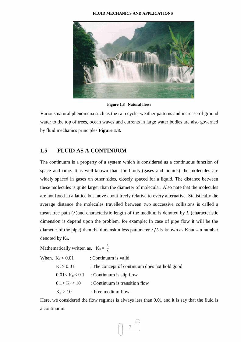
Figure 1.8 Natural flows
Various natural phenomena such as the rain cycle, weather patterns and increase of ground
water to the top of trees, ocean waves and currents in large water bodies are also governed
by fluid mechanics principles Figure 1.8.
1.5 FLUID AS A CONTINUUM
The continuum is a property of a system which is considered as a continuous function of
space and time. It is well-known that, for fluids (gases and liquids) the molecules are
widely spaced in gases on other sides, closely spaced for a liquid. The distance between
these molecules is quite larger than the diameter of molecular. Also note that the molecules
are not fixed in a lattice but move about freely relative to every alternative. Statistically the
average distance the molecules travelled between two successive collisions is called a
mean free path (𝜆)and characteristic length of the medium is denoted by L (characteristic
dimension is depend upon the problem. for example: In case of pipe flow it will be the
diameter of the pipe) then the dimension less parameter 𝜆/𝐿 is known as Knudsen number
denoted by Kn.
Mathematically written as, Kn = 𝜆
𝐿
When, Kn < 0.01 : Continuum is valid
Kn > 0.01 : The concept of continuum does not hold good
0.01< Kn < 0.1 : Continuum is slip flow
0.1< Kn < 10 : Continuum is transition flow
Kn > 10 : Free medium flow
Here, we considered the flow regimes is always less than 0.01 and it is say that the fluid is
a continuum.

FLUID MECHANICS AND APPLICATIONS
8
1.6 SHEAR STRESS AND NORMAL STRESS
Figure 1.9 Shear stress and Normal stress on the surface of a fluid element
In a Figure 1.9 small area dA considered on the surface of fluid element. The force
component Ft acting along the surface direction and the force component Fn acting normal
to the surface of the force F acting on the unity of surface are called Tangential Stress (𝜏-
Shear Stress) and Normal Stress(𝜎) respectively.
Mathematically it is given by,
The Normal Stress 𝜎 = lim𝑑𝐴→0
Fn
𝑑𝐴
And, Shear Stress 𝜏 = lim𝑑𝐴→0
Ft
𝑑𝐴
If a body in rest motion, the normal stress is called a Pressure.
1.7 FLUID DEFORMATIOM
Figure 1.10 Deformation of a fluid body
FLUID MECHANICS AND APPLICATIONS
9
Assume that a fluid with two parallel plates placed in a big container of water, the fluid
layer in contact with the upper plate. When shear stress 𝜏 applied on any location in a fluid,
the plate continuously is moving at the velocity of the plate no matter how it is small.From
the Figure 1.10 initially the fluid element at the position 0-1-1’, which is at rest, then it
will be followed by 0-2-2’ then to 0-3-3’ then to 0-4-4’ and so on. The tangential stress in a
fluid body depends on deformation of velocity and it will be decreases with the depth fluid
and reaching zero at the lower plate. It is done because of friction between each and every
fluid layers.
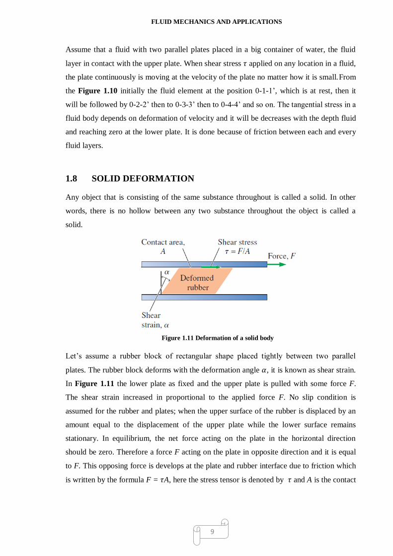
1.8 SOLID DEFORMATION
Any object that is consisting of the same substance throughout is called a solid. In other
words, there is no hollow between any two substance throughout the object is called a
solid.
Figure 1.11 Deformation of a solid body
Let’s assume a rubber block of rectangular shape placed tightly between two parallel
plates. The rubber block deforms with the deformation angle 𝛼, it is known as shear strain.
In Figure 1.11 the lower plate as fixed and the upper plate is pulled with some force F.
The shear strain increased in proportional to the applied force F. No slip condition is
assumed for the rubber and plates; when the upper surface of the rubber is displaced by an
amount equal to the displacement of the upper plate while the lower surface remains
stationary. In equilibrium, the net force acting on the plate in the horizontal direction
should be zero. Therefore a force F acting on the plate in opposite direction and it is equal
to F. This opposing force is develops at the plate and rubber interface due to friction which
is written by the formula F = 𝜏A, here the stress tensor is denoted by 𝜏 and A is the contact

FLUID MECHANICS AND APPLICATIONS
10
area between the rubber block and the upper plate. The rubber returns to its original
position if the force is removed.
1.9 DEFORMATION DIFFERENCE BETWEEN SOLID AND
FLUID
We divided any substance into two parts a solid and a fluid (gas, liquid) on the basis of
their ability to resist an applied shear (or tangential) stress that tends to change its shape.
Under the applied shear stress a solid is deforming, other side a fluid deforms continuously
under the influence of shear stress, no matter how small. So, from above experiments we
can says that,
(a) The elasticity of solid is shown in tension, compression and shearing stress
wherever fluids have only compressibility.
(b) Under constant shear force, in a solids stress is proportional to strain, but in a fluids
stress is proportional to strain rate.
(c) A solid is stops deforming at some fixed strain angle, but a fluid never stops
deforming and it approaches a certain rate of strain.
1.10 PROPERTIES OF FLUID
Any characteristic of a system is called a property. Some familiar properties are pressure P,
temperature T, volume V, and mass m. The list can be extended to more specific that
viscosity, density, Specific weight, etc… Now any properties can be divided into two parts,
intensive property or extensive property. Properties are independent of the mass of a
system is called intensive property. For example, Temperature, Pressure, Density,
etc...Properties are dependent of the mass of a system is called extensive property.
For example, total mass, total volume, total momentum, etc... We define some extensive
and intensive properties as below.
1.10.1 DENSITY / MASS DENSITY [ρ]
Density or Mass Density defined as the ratio between the mass of a fluid to its unit volume.
In other words, the mass per unit volume of a fluid is called density.
Density [ρ] = 𝑴𝒂𝒔𝒔 𝒐𝒇 𝒇𝒍𝒖𝒊𝒅
𝑽𝒐𝒍𝒖𝒎𝒆 𝒐𝒇 𝒇𝒍𝒖𝒊𝒅

FLUID MECHANICS AND APPLICATIONS
11
Unit of density is 𝐾𝑔
𝑚3 or 𝑔𝑚
𝑚3
At normal temperature density of water = 1 𝑔𝑚
𝑐𝑚3 . It is maximum at 40c.
At normal temperature density of air = 0.0013 𝑔𝑚
𝑐𝑚3
1.10.2 SPECIFIC WEIGHT/WEIGHT DENSITY [W]
Weight Density is defined as the ratio between the weights of fluid to its volume.
In other words, weight per unit volume of a fluid is called weight density.
W= weight of fluid
Volume of fluid
Unit of specific weight (in SI) is N/m3
1.10.3 SPECIFIC VOLUME[
𝟏
𝝆]
Specific volume is defined as the volume of a fluid occupied by a unit mass or volume per
unit mass.
𝟏
𝝆 =
Volume of fluid
Mass of fluid
Unit of specific volume is m3/Kg or m3/gm
1.10.4 SPECIFIC GRAVITY [S]
Specific volume is defined as the ratio of the weight density of a fluid to the weight density
of a standard fluid.
For a liquid, standard fluid is taken as water
For a gas, the standard fluid is taken air.
S (for liquid) = weight density of liquid
weight density of water
S (for gases) = weight density of gas
weight density of air
1.10.5 VISCOSITY [ 𝝁]
Viscosity is one of the most important fluid properties. Its impact we understood only in
case of the fluid is moving. When fluid is in motion the fluid elements move with different
velocities due to the friction of fluid within the elements. Hence due to this reason shear

FLUID MECHANICS AND APPLICATIONS
12
stress occurs between the fluid elements. Sir Isaac Newton gives the relationship between
the shear stress and the velocity gradient.
Figure 1.12 Velocity near solid boundary
Consider two layers of a fluid, the movement of one layer of fluid over another adjacent
layer of the fluid in same direction. When two layers of a fluid with distance ‘dy’ apart,
moving the top layer faster and tries to draw the lower slowly moving layer their different
velocities , say u and u + du respectively as show in Figure 1.12. The viscosity together
with relative velocity causes a shear stress acting between the fluid layers. By Newton’s
third law, the top layer causes a shear stress on the adjacent lower layer while the lower
layer causes a shear stress on the adjacent top layer. Newton postulated that this shear
stress is proportional to the rate of change of velocity with respect to y. It is denoted by
symbol τ (Tau).
du
dy
du
dy (1.1)
The proportionality relation in equation (1.1) between the shear stress and the rate of shear
strain is known as the constitutive equation or Newton’s law of viscosity. Common Fluids
such as water, air, mercury etc… satisfies Newton’s law of viscosity and are known as
Newtonian fluids.
On the other hand, toothpaste, blood, paints etc… do not obey this linear relationship
between τ and du
dy so are called Non-Newtonian fluids.

FLUID MECHANICS AND APPLICATIONS
13
Where, µ is the proportionality constant and it is called the coefficient of viscosity or
simply it is called the viscosity. It depends only on the nature of fluid (not on du or dy).
Sign of τ depends upon the sign of du
dy.
The relation between viscosity [ ] and temperature [t] is given by,
For liquid, 0 2
1
1 t t
For gas,
2
0 t t
From the above relation we conclude that:
For liquids, the viscosity µ is nearly independent of pressure and decreases rapidly with
increasing temperature. When we increase temperature in that case bonds between
molecules are becomes weak and since these bonds contribute to viscosity, the coefficient
of viscosity is decreased.
While in the case of gases, the viscosity is independent of pressure but it increase with
increasing temperature. Here we increase temperature intermolecular forces in gases are
not as an important factor in viscosity as collisions between the molecules and thus
increasing the coefficient of viscosity.
A striking result of the kinetic theory of gases is that the viscosity of a gas is independent
of the density of a gas. Viscosity is the principal factor resisting motion in laminar flow.
However, when the velocity has increased to the point at which the flow becomes
turbulent, pressure differences resulting from eddy currents rather than viscosity provide
the major resistance to motion. The value of viscosity is small for thin fluids, such as water
or air, but it takes large value in case of highly viscous fluid such as oil or glycerin.
Units of Viscosity
MKS Units: 𝐾𝑔
𝑚 . 𝑠𝑒𝑐
S.I. Units: Poise (the name after French Physician Jean Louis Marie Poiseuille,
1799-1869) or N.s/m2
C.G.S Unit of viscosity is Poise= dune-sec/cm2
1 Poise (P) = 0.1 𝐾𝑔
𝑚 . 𝑠𝑒𝑐 = 0.01 Pascal second (Pa.s)
1 Poise (P) = 100 Centipoises (Cp)

FLUID MECHANICS AND APPLICATIONS
14
1Cp =1 milliPascal second (mPa.s)
Table 1.1 Viscosity values for common fluids at room temperature
Substance Viscosity
(𝝁 − 𝒎𝑷𝒂. 𝒔)
Air 0.01
Water 1
Castor oil 6× 10²
Olive oil 102
Honey 104
Corn syrup 105
Mercury 1.5
Ethyl alcohol 1.2
Bitumen 1.08× 10⁵
1.10.6 KINEMATIC VISCOSITY [𝛎]
The effect of viscosity on the motion of a fluid is determined by the ratio of dynamic
viscosity µ to the density ρ rather than by µ alone. This ratio is known as ‘kinemtic
viscosity’ denoted by ν.
In other words, Viscosity per unit density is called Kinematic Viscosity.
Mathematically it is written as, 𝜈 = 𝐷𝑦𝑛𝑒𝑚𝑖𝑐 𝑣𝑖𝑠𝑐𝑜𝑠𝑖𝑡𝑦
𝐷𝑒𝑛𝑠𝑖𝑡𝑦=
𝜇
𝜌
Units of kinematic viscosity
S.I. Unit: m2/s
C.G.S. unit: stoke = cm2/s , The named after George Gabriel Stokes
1 stoke (St)=10-4 m2/s
1 centistokes (cst) = 10-6 m2/s
1.10.7 APPARENT VISCOSITY
Apparent viscosity is the slope of the sharing stress versus rate of strain which varies with
the rate of strain for non-Newtonian fluids. For Newtonian fluids, the apparent viscosity is
the same as the dynamic viscosity (or simply viscosity).

FLUID MECHANICS AND APPLICATIONS
15
Mathematically written it is as,
1
n
dy
duk
dydu
1.10.8 NO-SLIP CONDITION
Through experimental observations it is established that, the relative velocity between the
solid surface and the adjacent fluid particles is becomes zero. In other words, we can say
that the fluid elements in contact with a stationary surface attain the velocity of the surface.
It is known as the “no-slip” condition. Also it is note that this behaviour of no-slip at the
solid surface should not be confused with the wetting of surfaces by the fluids. For
example, mercury flowing in a stationary glass tube will not wet the surface, but will have
zero velocity at the wall of the tube. The wetting property results from surface tension,
whereas the no-slip condition is a consequence of fluid viscosity.
The velocity and the temperature of fluid at a point of contact with solid surface is same as
the velocity and temperature of that solid surface,
(V)fluid = (V)wall and (T)fluid = (T)wall
These conditions are called the no-slip condition or no temperature-jump condition. These
conditions are used as boundary conditions in the analysis of fluid flow past a solid
surface.
1.10.9 BOUNDARY LAYERS
The boundary layer concept was first introduced by Ludwig Prandtl, a German
aerodynamicist, in 1904. Let us now follow the impact as a flow approaches a solid body,
to make it simple. Consider a flat plate shown in Figure 1.13.
Figure 1.13 Formation of a Boundary Layer

FLUID MECHANICS AND APPLICATIONS
16
Figure 1.14 Free stream layer and boundary layer for flow past a flat plate
A uniform flow (inviscid flow) with velocity 𝑈∞ was applied in the front of a flat plate. As
soon as the flow 'hits' the plate No Slip Conditions gets into action. As a result, the velocity
on the body becomes zero. Since the effect of viscosity is to resist fluid motion, the
velocity closed to the solid surface continuously decreases towards downstream. But away
from the flat plate the speed is equal to the free stream value 𝑈∞ (Figure 1.14).
Consequently a velocity gradient is set up in the fluid in a direction of normal to the flow
direction. Also the component of velocity gradient in a direction normal to the surface is
large as compared to the velocity gradient in the stream wise direction. However, outside
the boundary layer where the effect of the shear stresses on the flow is small compared to
values inside the boundary layer (since the velocity gradient 𝜕𝑢
𝜕𝑦 is negligible).
In the normal direction, within this thin layer, the gradient 𝜕𝑢
𝜕𝑦 is very large compared to the
gradient in the flow direction.
1.11 TYPES OF FLUID
Fluid is basically classified into following five categories:
1.11.1 IDEAL FLUID
A fluid, which is not compressible and inviscid is known as an ideal fluid. Since all real
fluid has some viscosity, Ideal fluid (perfect fluid) is only an imaginary fluid.
1.11.2 REAL FLUID
A viscous fluid is known as Real fluid (Practical fluid). All the existing fluids are real
fluids.

FLUID MECHANICS AND APPLICATIONS
17
1.11.3 NEWTONIAN FLUID
A real fluid, in which the shear stress is directly proportional to the rate of shear strain
(velocity gradient), known as a Newtonian fluid. i.e. Fluids which obey the Newtonian law
of viscosity are known as Newtonian fluids. For example: Water, air, Kerosene, metals,
salts, etc…
Graph of all type fluids shown in Figure 1.15.
Figure 1.15 Types of fluid
1.11.4 NON- NEWTONIAN FLUIDS
A real fluid, in which the shear stress is directly not proportional to the rate of shear strain
(velocity gradient), known as Non-Newtonian fluid. i.e. Fluids which do not obey the
Newtonian law of viscosity are called Non- Newtonian Fluids.
For Example: Printer ink, blood, mud, slurries, polymer solutions, etc….
1.11.5 IDEAL PLASTIC FLUID
A fluid, in which the shear stress is more than the yield value and then it is proportional to
the rate of shear strain (velocity gradient) such fluid known as an Ideal plastic fluid.

FLUID MECHANICS AND APPLICATIONS
18
1.12 DETAILED FOR NON-NEWTONIAN FLUID
Any fluids are classified in two different ways; either according to their response to the
externally applied pressure or according to the effects produced under the action of a shear
stress.
According to the first scheme of classification fluids are called ‘compressible’ and
‘incompressible’ fluids, depending upon whether or not the volume of an element of fluid
is dependent on its pressure. A gas possesses compressibility influence the flow
characteristics, while a liquid possesses an incompressible influence the flow
characteristics. Compared to the first scheme the effects of shearing which is of greater
importance.
Due to most common fluid property viscosity, when the fluid elements move with different
velocities, each element will feel some resistance due to fluid friction within the elements.
Therefore shear stress can be identified between the fluid elements with different
velocities. The relationship between the shear stress and the velocity gradient was given by
Sir Isaac Newton. It is known as Newton’s law of viscosity and expressed as in equation
(1.1).
In general, the viscosity of a fluid depends on both temperature and pressure, although the
dependence on pressure is rather weak. For liquids, both the dynamic and kinematic
viscosities are practically independent of pressure, and any small variation with pressure is
usually disregarded, except at extremely high pressures.
In a Newtonian fluid, the relation between the shear stress and the shear rate is linear as
shown in equation (1.1). In a non-Newtonian fluid, the relation between the shear stress
and the shear rate is not linear and can even be time-dependent. This general relationship
can be expressed as equation (1.2), Therefore a constant coefficient of viscosity cannot be
defined.
( )
n
duA B t
dy
(1.2)
Therefore, the apparent viscosity (shear stress/shear rate) is not constant at a given pressure
and temperature. It depends on flow geometry, shear rate, etc. and sometimes even on the

FLUID MECHANICS AND APPLICATIONS
19
kinematic history of the fluid particles under consideration.Such materials can be divided
into the below three general classes:
(a) Fluids for which the shear rate at a point is decided only by the value of the shear stress
at that point. These fluids are known as unsteady or purely viscous or inelastic or
generalized Newtonian Fluids (GNF).
(b) Fluids for which the relation between shear stress and shear rate depends, in addition,
upon the shearing duration and their kinematic history; they are known as time-
dependent fluids.
(c) System exhibiting characteristics of both ideal fluids and elastic solids and showing
partial elastic recovery, after deformation; these are categorized as visco-elastic or
elastic-viscous fluids.
Again further classification of purely viscous and visco-elastice fluids are shown in Table
1.2 and there graph for shear stress versus shear rate is shown in Figure 1.16.
Table: 1.2 Classification of Non Newtonian fluids
Non- Newtonian Fluid ( )
n
duA B t
dy
Purely Viscous Fluids visco-elastice Fluids
Time- Independent Time- Dependent
Visco - elastice fluids
duA B
dy
Example: Liquid and
solid combinations in
pipe
1. Pseudo Plastic
, 1
n
duA n
dy
Example: Blood , Milk
2. Dilatant Fluids
, 1
n
duA n
dy
Example: Butter
3. Bingham or
Ideal Plastic Fluids
0
n
duA
dy
Example: Water suspensions of
clay and flyash
1. Thixotropic fluids
( )
n
duA B t
dy
Where, B(t) is decreasing
Example: Printer Ink, Crude oil
2. Rheopectic Fluids
( )
n
duA B t
dy
Where, B(t) is increasing
Example: Rare liquid solid
suspension

FLUID MECHANICS AND APPLICATIONS
20
The graph of the shear stress versus shear rate will not remain constant by changing the
shear rate. Fluids are known as Pseudo plastic fluid (shear-thinning) for which the viscosity
decreases with the increase in shear rate. While in the dilatants fluids (shear-thickening)
viscosity will be increase with the increase of shear rate.
Figure 1.16 Shear stress vs Shear rate
Shear-thinning behaviour is more common than the shear-thickening. A graph of shear
thinning fluid and shear thickening fluid for shear stress versus shear rate is given by
Figure 1.17 and Figure 1.18 respectively.
Figure 1.17 Graph for Shear-thinning fluid Figure 1.18 Graph for Shear-thickening fluid
Examples of shear-thinning fluids are polymer melts such as molten polystyrene, polymer
solutions such as polyethylene oxide in water and some paints. Paint flows comfortably
when it is sheared with a brush. But if the shear stress is removed, it cannot flow easily
because of the increase in viscosity. Of course the solvent evaporates soon and then the

FLUID MECHANICS AND APPLICATIONS
21
point sticks to the surface. The behaviour of paint is a bit more complex than this, because
at a given shear rate, the viscosity changes with time.
Visco-elastice behaviour is another important class of non-Newtonian fluids. Fluid falls in
this category behave both of solid (elastic) and fluids (viscous). These fluids will not flow
on applying a small shear stress. In other words it behave as a solid still yield stress 0 , the
shear stress must exceed 0 the fluid is flow.
Consider the simple example of toothpaste. It would be good if the paste does not flow at
the slightest amount of shear stress. We need to apply an adequate force before the
toothpaste will start flowing. So, visco-plastic fluids behave like solids when the applied
shear stress is less than the yield stress. Once it exceeds the yield stress, the visco-plastic
fluid will flow just like a fluid. Bingham plastics are a special class of visco-plastic fluids
that exhibit a linear behavior of shear stress against shear rate. Typical visco-plastic
behaviors are illustrated in Figure 1.19.
Figure 1.19 Visco-plastic behaviours
More examples of Visco-plastic fluids are drilling mud, nuclear fuel slurries, egg-white,
mayonnaise, blood. Also, some paints exhibit a yield stress. Several industrially important
polymers melt and solutions are viscoelastic.
Well this is not an adequate discussion for the behaviour of non-Newtonian fluids. Some
fluids of this category are having time dependent behaviour. That is the viscosity of fluid
may change with time under a given constant shear rate. In the case of thyrotrophic fluid,
the viscosity will decrease with time even under a constant applied shear stress. However,

FLUID MECHANICS AND APPLICATIONS
22
when the stress is removed, the viscosity will gradually recover with time as well. For the
rheoplastic fluid the viscosity increases with time when a constant shear stress is applied.
1.13 TYPES OF FLUID FLOW
1.13.1 VISCOUS AND INVISCID FLOW
Figure-1.20 Viscous and inviscid flow region
When two fluid layers move relative to each other, a friction force will be develop between
them and the slower layer tries to slow down the faster layer. This internal resistance to
flow is quantified by the fluid property viscosity, which is a measure of internal stickiness
of the fluid. Viscosity is caused by cohesive forces between the molecules in liquids and by
molecular collisions in gases. There is no fluid with zero viscosity, and thus all fluid flows
involve viscous effects to some degree. Flows in which the frictional effects are significant
are called viscous flows however, in many flows in practical interest, there are regions
(typically regions not close to solid surfaces) where viscous forces are negligibly small
compared to inertial or pressure forces. Neglecting the viscous terms in such inviscid flow
regions greatly simplifies the analysis without much loss in accuracy. The development of
viscous and inviscid regions of flow as a result of inserting a flat plate parallel into a fluid
stream of uniform velocity is shown in Figure 1.20. The fluid sticks to the plate on both
sides because of the no-slip condition, and the thin boundary layer in which the viscous
effects are significant near the plate surface is the viscous flow region. The region of flow

FLUID MECHANICS AND APPLICATIONS
23
on both sides away from the plate and unaffected by the presence of the plate is the
inviscid flow region.
1.13.2 INTERNAL AND EXTERNAL FLOW
Figure-1.21 External flow over tennis ball and gives the turbulent flow behind
A fluid flow is classified as being internal or external, depending on whether the fluid is
forced to flow in a confined channel or over a surface. The flow of an unbounded fluid
over a surface such as a plate, a wire or a pipe is called external flow. The flows of water in
rivers and irrigation ditches are examples of type of flow. The flow in a pipe or duct
completely bounded by solid surfaces is called internal flow. In external flows the viscous
effects are limited to boundary layers near solid surfaces and to wake regions downstream
of bodies. In Figure 1.21 shows that external flow over tennis ball and gives the turbulent
flow behind.
1.13.3 COMPRESSIBLE AND INCOMPRESSIBLE FLOW
A fluid is classified into compressible or incompressible depending upon the level of
variation of density during the fluid flow. A flow is said to be an incompressible if the
density remains constant throughout fluid flow. Therefore, the volume of every portion of
fluid remains unchanged over the course of its motion. The density of liquid is constant
thus the flow of liquids is usually referred to as incompressible substances at pressure of
210 atm. On the other hand, gases are highly compressible fluid. When analyzing rockets,

FLUID MECHANICS AND APPLICATIONS
24
spacecraft, and other systems that involve high-speed gas flows, the flow speed is often
expressed in terms of the dimensionless Mach number defined in 1.14.3.
When Liquid flows are incompressible to a high level of accuracy, but the level of
variation in density in gas flows and the consequent level of approximation made when
modelling gas flows as incompressible depends on the Mach number. Gas flows can often
be approximated as incompressible if the density changes are under about 5 percent, which
is usually the case when Ma < 0.3. Therefore, the compressibility effects of air can be
neglected at speeds under about 100 m/s. Note that the flow of a gas is not necessarily a
compressible flow.Compressibility effects are very important in the design of modern
high-speed aircraft and missiles, power plants, fans and compressors.
1.13.4 LAMINAR AND TURBULENT FLOW
Figure-1.22 Laminar, Transitional and Turbulent Flows
Some flows are smooth and orderly while others are rather chaotic. The highly ordered
fluid motion characterized by smooth layers of fluid is called laminar. The word laminar
comes from the movement of adjacent fluid particles together in “laminates.” The flow of
high-viscosity fluids such as oils at low velocities is typically laminar. The highly
disordered fluid motion that typically occurs at high velocities and is characterized by

FLUID MECHANICS AND APPLICATIONS
25
velocity fluctuations is called turbulent (Figure 1.22). The flow of low-viscosity fluids
such as air at high velocities is typically turbulent. The flow regime greatly influences the
required power for pumping. A flow that alternates between being laminar and turbulent is
called transitional The experiments conducted by Osborn Reynolds in the 1880s resulted in
the establishment of the dimensionless Reynold’s number (Re) as the key parameter for the
determination of the flow regime in pipes.
When, Re ≤2000; the pipe flow is laminar.
Re >2000; the pipe flow is turbulent.
1.13.5 NATURAL (OR UNFORCED) AND FORCED FLOW
A fluid flow is said to be natural or forced, depending on how the fluid motion is initiated.
In force flow a fluid is forced to flow over a surface or in a pipe by external means such as
a pump or a fan. In natural flows any fluid motion is due to natural means such as the
buoyancy effect, which manifests itself as the rise of the warmer (and thus lighter) fluid
and the fall of cooler (and thus denser) fluid. In solar hot-water systems, for example, the
thermo siphoning effect is commonly used to replace pumps by placing the water tank
sufficiently above the solar collectors.
1.13.6 STEADY AND UNSTEADY FLOW
The terms steady and unsteady are used frequently in engineering, thus it is important to
have a clear understanding of their meanings. The term steady implies no change at a point
with time. The opposite of steady is unsteady.
Figure-1.23(a) Unsteady flow Figure-1.23(b) Steady flow

FLUID MECHANICS AND APPLICATIONS
26
Many devices such as turbines, compressors, boilers, condensers, and heat exchangers
operate for long periods of time under the same conditions, and they are classified as
steady-flow devices. During steady flow, the fluid properties can change from point to
point within a device, but at any fixed point they remain constant. Therefore, the volume,
the mass, and the total energy content of a steady-flow device or flow section remain
constant in steady operation. Steady-flow conditions can be closely approximated by
devices that are intended for continuous operation such as turbines, pumps, boilers,
condensers, and heat exchangers of power plants or refrigeration systems. Some cyclic
devices, such as reciprocating engines or compressors, do not satisfy the steady-flow
conditions since the flow at the inlets and the exits is pulsating and not steady. However,
the fluid properties vary with time in a periodic manner, and the flow through these devices
can still be analyzed as a steady-flow process by using time-averaged values for the
properties. Some fascinating visualizations of fluid flow are provided. A nice illustration of
an unsteady-flow field is shown in Figure 1.23(a), taken from Van Dyke’s book. Figure
1.23(b) is an instantaneous snapshot from a high-speed motion picture; it reveals large,
alternating, swirling, turbulent eddies that are shed into the periodically oscillating wake
from the blunt base of the object. The eddies produce shock waves that move upstream
alternately over the top and bottom surfaces of the airfoil in an unsteady fashion. The
resulting time-averaged flow field appears “steady” since the details of the unsteady
oscillations have been lost in the long exposure.
1.14 SOME FLUID NUMBERS
In the governing equations of fluid flow non-dimensionalization takes an important role in
the both theoretical and computational reasons. Non-dimensional scaling provides a
physical insight into the importance of various terms in the system of governing equations.
Computationally, dimensionless forms have the added benefit of providing numerical
scaling of the system discrete equations, thus providing a physically linked technique for
improving the ill-conditioning of the system of equations. Moreover, dimensionless forms
also allow us to present the solution in a compact way. Some of the important
dimensionless numbers used in fluid mechanics, gas dynamics and heat transfer are given
below.

FLUID MECHANICS AND APPLICATIONS
27
1.14.1 PRANDTL NUMBER (Pr)
The dimensionless number Prandtl Number (the named after the German
physicist Ludwig Prandtl ) is defined as the ratio of momentum diffusivity and thermal
diffusivity.
In other words, the thermal boundary layer thickness is similarly the distance from the
body at which the temperature is 99% of the temperature found from an inviscid solution.
The ratio of the two thicknesses (velocity boundary layer and thermal boundary layer ) is
governed by the Prandtl number.
Mathematically written as, viscous diffusion rate \ Cp
Pr = thermaldiffusion rate k \ (Cp ) k
Where, 𝛼 = Thermal diffusivity (SI units: m2/s).
Cp = Specific heat (SI units: J/kg-K).
𝜇 = Dynamic Viscosity (SI units: Pa s = N s/m2).
K = Thermal conductivity (SI units: W/m-K).
𝜌 = Density (SI units: kg/m3).
When, Pr = 1 : the two boundary layers are the same thickness.
Pr > 1 : the thermal boundary layer is thinner than the velocity boundary layer.
Pr < 1 : the thermal boundary layer is thicker than the velocity boundary layer
(which is the case for air at standard conditions).
Pr << 1 : the thermal diffusivity (heat) dominates the behavior.
Pr >> 1 : the momentum diffusivity (velocity) dominates the behavior.
It is used in heat transfer and free and forced convection calculations and which is depends
only on fluid and its properties.
In heat transfer problems, the Prandtl number controls the relative thickness of the
momentum and thermal boundary layers. When Pr is small, it means that the heat diffuses
quickly compared to the velocity (momentum). This means that for liquid metals the
thickness of the thermal boundary layer is much bigger than the velocity boundary layer.
For example, liquid mercury indicates that the heat conduction is more significant
compared to convection so thermal diffusivity is dominant. for engine oil, convection is

FLUID MECHANICS AND APPLICATIONS
28
very effective in transferring energy from an area in comparison to pure conduction, so
momentum diffusivity is dominant.
Table 1.3 Some typical values for Pr
Substance Prendtl Number (Pr)
Air 0.7-0.8
Oxygen 0.63
Water 7
Engine Oil 100-40000
Glycerol 1000
Polymer melts 10000
1.14.2 REYNOLDS NUMBER (Re)
The dimension less number, the ratio of inertial forces to viscous forces is known as the
Reynolds number.
The concept of Reynolds Number was introduced by Sir George Stokes in 1851 but the
Reynolds number was named by Arnold Sommerfeld in 1908 after Osborne Reynolds
(1842-1912), who popularized its use in 1883.
Mathematically written as,
2
2
e
VInertail force VD VDDR
VViscous forceD
Where, V = the flow velocity (m/s).
D = characteristic linear dimension (m).
ρ = fluid density (kg/m3).
μ = dynamic viscosity (Pa.s).
ν = kinematic viscosity (m2/s).
It is a convenient parameter for predicting if a flow condition will be laminar or turbulent
(flow pattern). It can be interpreted that when the viscous forces are dominant (slow flow,
low Re, Re < 2000) they are sufficient enough to keep all the fluid particles in line, and
then the flow is laminar. Even very low Re indicates viscous creeping motion, where
inertia effects are negligible. When the inertial forces dominate over the viscous forces

FLUID MECHANICS AND APPLICATIONS
29
(when the fluid is flowing faster and Re >4000) then the flow is turbulent and 2000<Re
<4000 then flow is transition.
0 < Re < 1 : highly viscous laminar “creeping” motion.
1 < Re < 100 : Laminar, strong Reynolds number dependence.
100 < Re < 103 : Laminar boundary Layer theory useful.
103 < Re < 104 : transition or turbulence.
104 < Re < 106 : turbulent, moderate Reynolds number dependence.
106 < Re < : turbulent, slight Reynolds number dependence.
1.14.3 MACH NUMBER (Ma)
The flow speed is often expressed in terms of the dimensionless number is known as Mach
in honour of Ernst Mach, a late 19th century physicist who studied gas dynamics. The
Mach number Ma allows us to define flight regimes in which compressibility effects vary.
Mach number defined as,
Ma = 𝑉
𝐶 =
𝑆𝑝𝑒𝑒𝑑 𝑜𝑓 𝐹𝑙𝑜𝑤
𝑆𝑝𝑒𝑒𝑑 𝑜𝑓 𝑠𝑜𝑢𝑛𝑑
Where, c = The speed of sound
= 346 m/s in air at room temperature at sea level.
When Ma<0.8 : the flow is Subsonic
0.8<Ma<1.2 : the flow is transonic
Ma =1 : the flow is sonic
1.2<Ma <5 : the flow is supersonic
5<Ma <10 : the flow is hypersonic
Ma >10 : the flow in hypervelocity
The trigonometric sine of the cone angle b is equal to the inverse of the Mach number M
and the angle is therefore called the Mach angle.
Sin (b) = 1 / Ma
1.15 TIME LINE, PATH LINE, STREAK LINE AND STREAMLINES
In the analysis of problems in fluid mechanics, frequently it is advantageous to obtain a
visual representation of a flow field. Such representation is provided by timelines, path
lines, streak lines and streamlines.If a number of adjacent fluid particle in a flow field are

FLUID MECHANICS AND APPLICATIONS
30
marked at a given instant, they form a line in the fluid at that instant; this line is called
timeline see Figure 1.24.
A path line is the path or trajectory traced out by a moving fluid particle see Figure 1.25.
To make a path line visible, we might identity a fluid particle at a given instant e.g. by the
use of dye, and then take a long exposure photograph of its subsequent motion. The line
traced out by the particle is a path line.
Figure1.24 Timeline Figure 1. 25 Path lines
On the other hand, we might choose to focus our attention on a fixed location in space and
identify again by the use of dye, all fluid particles passing through this point. After a short
period of time we would have a number of identifiable fluids particles in the flow, all of
which had, at some time, passes through one fixed location in space. The line joining these
fluid particles is defined as a streak lines see Figure 1.26.
Streamlines are lines drawn in the flow field so that a given instant they are tangent to the
direction of flow at every point in the flow field. Since the streamlines are tangent to the
velocity vector at every point in the flow field, there can be no flow across a streamline see
Figure 1.27.
Figure 1.26 Streaklines Figure 1.27 Streamlines

FLUID MECHANICS AND APPLICATIONS
31
Thus, streamline define at a single instant in a flow do not intersect. In steady flow, the
velocity at each point in the flow field remains constant with time and consequently, the
streamlines do not vary from one instant to the next. This implies that a particle located on
a given streamline will remain on the same streamline. Furthermore, consecutive particles
passing through a fixed point in space will be on the same streamline and, subsequently
will, remain on this streamline. Thus in a steady slow, path line, streakiness and
streamlines are identical lines in the flow field.
The shape of the streamlines may vary from instant if the flow in unsteady. In the case of
unsteady flow, path lines streamlines and streak lines do not coincide.
1.16 STREAM FUNCTION :
A continuous function tyx ,, called the stream function, that replace the two velocity
components u (x, y, t) and v (x, y, t) along the x and y direction respectively.
u and vy x
The stream function is a device which allows us to wipe out the contenting equation and
solve the momentum equation directly for the single variable .

CHAPTER-2
GOVERNING EQUATIONS AND FLUID
MODELS
2.1 SYSTEM
Figure 2.1 System types
In the analysis of problem the quantity of matter in the space is known as a system. The
external part of the system is called the surrounding part and system is separated from
surrounding part is called boundary of the system Figure 2.1. This boundary may be solid
or imaginary and may be moving or fixed.
Any System is divided into three types as follows:
2.1.1 CONTROL VOLUME SYSTEM (OPEN SYSTEM)
There is no any change in the volume of the system mass and energy crosses the boundary
of the system is called control volume system. In general, Most of the engineering devices
are open system.
2.1.2 CONTROL MASS SYSTEM (CLOSED SYSTEM)
The system having fixed mass with fixed identity. In other wards we can say that there is
no mass transfer in the system is called control mass system.

GOVERNING EQUATIONS AND FLUID MODELS
33
2.1.3 ISOLATED SYSTEM
The system in which neither energy nor mass interact between the systems and the
surrounding is called isolated system. In other words, it is a fixed mass and fixed energy
with same identity.
2.2 THE DIFFERENTIAL EQUATION OF CONSERVATION OF
MASS (CONTINUITY EQUATION)
There is no accumulation of mass. In other words, Mass is neither created nor destroyed in
the fluid element is known as the conservation of Mass law. The equation based on the
principle of the conservation of mass is known as equation of continuity. For finding all
basic differential equations of motion either an elemental system or an elemental control
volume is considered.
Figure 2.2 Elemental fixed control volumes in Cartesian coordinate system
Let us consider one fluid element having length dx, dy and dz in the direction of x, y and z
respectively and u, v and w are the in late velocity component along x, y and z direction
respectively.
Mass entering in the phase ABCD per second = AV
Area of ABCD Velocity in x direction
dy dz u
Mass living in the phase EFGH per second dy dz u dy dz u dxx

GOVERNING EQUATIONS AND FLUID MODELS
34
Therefore, Rate of increase in mass x-direction
Mass entering in Mass living in
the phase ABCD the phase EFGH
per second per second
dy dz u dy dz u dy dz u dxx
dy dz u dy dz u dy dz u dxx
u dxdy dzx
Similarly,
Rate of increase in mass y-direction v dxdy dzy
Rate of increase in mass z-direction w dxdy dzz
Total rate of increase in mass u dxdy dz v dxdy dz w dxdy dzx y z
Now by conservation of mass law, mass is neither created nor destroyed in the fluid
element. So, net increase of mass per unit time in the fluid element must equal to the total
rate of increased mass in the fluid element.
dxdy dz u dxdy dz v dxdy dz w dxdy dzt x y z
The volume element term (dx dy dz) cancelled out on both the sides. We get partial
differential equation having the partial derivatives of velocity components and density of
fluid.
0u v wt x y z
(2.1)
The equation (2.1) called The Equation of Continuity. It is valid for an infinitesimal
control volume system. Because it do not required any assumptions except that the density
and velocity are continuum functions. In other words we can say that this equation satisfies
for the flow of types steady, unsteady, viscous, frictionless, compressible Or
incompressible.
Also, we know from the definition of divergence of a vector V.
Vwz
vy
uu
(2.2)
Substitute the value of equation (2.2) in equation (2.1) we have

GOVERNING EQUATIONS AND FLUID MODELS
35
0
V
t
(2.3)
Cylindrical Polar Coordinates:
In cylindrical polar coordinates continuity equation (2.1) written as,
011
zr v
zv
rvr
rrt
(2.4)
Compressible and Steady Flow:
For steady flow, 0t
So, equation (2.1) and (2.4) reduce as,
Cartesian coordinate:
0
w
zv
yu
x
(2.5)
Cylindrical coordinate:
011
zr v
zv
rvr
rr
(2.6)
Incompressible flow:
For incompressible flow the density changes are negligible with respect to time so
equations (2.5) and (2.6) are reduced as,
Cartesian coordinate: 0u v w
x y z
(2.7)
Cylindrical coordinate:
011
zr v
zv
rvr
rr
(2.8)
2.3 FORCES ACTING ON THE SYSTEM
2.3.1 INERTIA FORCE (Fi)
The product of the mass of fluid element and its acceleration is defined as inertia force.
Mass of the Fluid element 3l where, 𝑙 = the characteristic dimension

GOVERNING EQUATIONS AND FLUID MODELS
36
Acceleration of the Fluid element
2v v
t l
lt
v
So, the magnitude of 2 2
iF ma l v
2.3.2 VISCOUS FORCE (Fv)
Due to shear stress the viscous force arising in flow of fluid.
Therefore, Shear stress = rate of shear strain x viscosity
= velocity gradient x viscosity
v
l
Magnitude of vF = the surface area at which the shear stress applied shear stress
2v
ll
v l
2.3.3 PRESSURE FORCE (Fp)
Due to the difference of pressure, the pressure force arising in a flow field.
Mathematically it is written as, 2
pF p l
2.3.4 GRAVITY FORCE (Fg)
Due to the weight (gravitational attraction) of the fluid element the gravity force arising in
a flow field.
Mathematically it is written as, 3
gF l g
2.3.5 CAPILLARY FORCE (SURFACE TENSION FORCE) (Fc)
The capillary force arises due to the existence of an interface between two fluids. The
surface tension force acting in the direction of tangent to a surface is the product of the
length (l) of a linear element on the surface perpendicular to which the force acts and the
coefficient of surface tension (𝜎).
Mathematically it is written as, cF l

GOVERNING EQUATIONS AND FLUID MODELS
37
2.3.6 COMPRESSIBILITY FORCE (ELASTIC FORCE) (Fe)
Due to the consideration of compressibility of the fluid force elastic force comes into its
flow. When we compressed the fluid (a decrease in volume), the increase in pressure is
directly proportional to the bulk modulus of elasticity and gives rise to a such force known
as the elastic force.
Mathematically it is written as,
2
eF E l
2.4 DYNAMIC SIMILARITY
In general, the flow of a fluid does not involve all the forces simultaneously. Therefore the
dimensionless parameter dynamic similarity is defined. It is defined as the ration of
dominant forces causing on the flow. Some of the examples are given in the following
Table-2.1.
Table 2.1 Dynamic similarity
Ratio of the forces
Pertinent dimensionless term
as the criterion of dynamic
situations of fluid flow
Name Recommended
symbol
𝐼𝑛𝑒𝑟𝑡𝑖𝑎 𝑓𝑜𝑟𝑐𝑒
𝑉𝑖𝑠𝑐𝑜𝑢𝑠 𝑓𝑜𝑟𝑐𝑒
𝜌 𝑙 𝑉
𝜇
Reynolds
number Re
𝑃𝑟𝑒𝑠𝑠𝑢𝑟𝑒 𝑓𝑜𝑟𝑐𝑒
𝐼𝑛𝑒𝑟𝑡𝑖𝑎 𝑓𝑜𝑟𝑐𝑒
∆𝑝
𝜌 𝑉2 Euler number Eu
𝐼𝑛𝑒𝑟𝑡𝑖𝑎 𝑓𝑜𝑟𝑐𝑒
𝐺𝑟𝑎𝑣𝑖𝑡𝑦 𝑓𝑜𝑟𝑐𝑒
𝑉
(√𝑙𝑔) Froude number Fr
𝑆𝑢𝑟𝑓𝑎𝑐𝑒 𝑡𝑒𝑛𝑠𝑖𝑜𝑛 𝑓𝑜𝑟𝑐𝑒
𝐼𝑛𝑒𝑟𝑡𝑖𝑎 𝑓𝑜𝑟𝑐𝑒
𝜎
𝜌 𝑉2𝑙 Weber number Wb
𝐼𝑛𝑒𝑟𝑡𝑖𝑎 𝑓𝑜𝑟𝑐𝑒
𝐸𝑙𝑎𝑠𝑡𝑖𝑐 𝑓𝑜𝑟𝑐𝑒
𝑉
√𝐸𝑠𝜌⁄
Mach number Ma
2.5 NAVIER-STOKES DIFFERENTIAL EQUATION
Generalized equations of motion of a real flow are named after its inventors (Navier and
Stokes) known as Navier-Stokes equations. These equations are derived using the

GOVERNING EQUATIONS AND FLUID MODELS
38
Newton’s second law of motion. Which states that, the external forces acting on a body
parts is equals to the product of mass and acceleration.
Now, there are two types of external forces acting on the body:
1. Force acting throughout the mass of a body. This includes gravitational force and
electromagnetic force.
2. Force acting on the boundary. This includes pressure force and frictional force.
Let us consider per unit mass body force is,
ˆˆ ˆb x y zf i f j f k f (2.9)
And per unit volume surface force is,
ˆˆ ˆs sx sy szf i f j f k f (2.10)
Figure 2.3 Stress components and their location in a fluid element
From the flow of fluid consider a differential fluid element shown in Figure 2.3. fsx denotes
the surface force acting on the face ABCD per unit area and defined as,
ˆˆ ˆsx x xy xzf i j k
And the surface force acting on the face BFGC per unit area is given by,
sx
sx
ff dx
x

GOVERNING EQUATIONS AND FLUID MODELS
39
Due to imbalance of surface forces the resultant force acting on the body is given by,
sxfdx dy dz
x
Similarly, the resultant total surface forces acting on all six surfaces is,
sysx szff f
dx dy dzx y z
Therefore, total net surface force df per unit volume is
sysx szff f
dfx y z
(2.11)
Now the surface force acting on any surface is given by two components, 𝜏-shearing
stresses and 𝜎- normal stresses. Given by the equation,
ˆˆ ˆ
ˆˆ ˆ
ˆˆ ˆ
s x x x y x z
s y y x y y z
s z z x z y z
f i j k
f i j k
f i j k
(2.12)
These three surface force components contain nine scalar quantities and its form a stress
tensor. The set of this nine stress tensor component can be written as in matrix notation,
x xy xz
yx y yz
zx zy z
A
(2.13)
Here stress tensor matrix A is symmetric.
Take the rotation of the fluid element about y-axis then,
( ) ( )
( )
y y xz zx
xz xz
dI dydz dx dxdy dz
dx dy dz
(2.14)
Where, 𝜔�̇� = angular acceleration about y-axis
dIy = moment of inertia about y-axis
Now in left hand side of above equation (2.14) contains fifth power of linear dimensions,
and right side third power of linear dimensions which is contradict the element to a point.
So it is true only in case of 𝜏𝑥𝑧 = 𝜏𝑧𝑥. Similarly by considering remaining two axis we get
𝜏𝑥𝑦 = 𝜏𝑦𝑥 and 𝜏𝑧𝑦 = 𝜏𝑦𝑧.

GOVERNING EQUATIONS AND FLUID MODELS
40
Combining equation (2.11) and equation (2.12), the total net surface force acting per unit
volume is given by,
ˆ ˆ
ˆ
xy xy y yzx xz
s
yzxz z
df i jx y z x y z
kx y z
(2.15)
For velocity field,
ˆˆ ˆDV Du Dv Dwi j k
Dt Dt Dt Dt (2.16)
By Newton’s second laws of motion applied to the differential element we get,
( ) (df )( ) ( )s b
DVdx dy dz dx dy dz f dx dy dz
Dt
Or fs b
DVd f
Dt (2.17)
Substitute equation (2.16), (2.15) and (2.9) in equation (2.17) we obtain
xyx xz
x
Duf
Dt x y z
(2.18a)
xy y yz
y
Dvf
Dt x y z
(2.18b)
yzxz z
z
Dwf
Dt x y z
(2.18c)
According to Stokes’ laws of viscosity, shear stress is directly proportional to normal
stresses and rate of shear strain which is given by
xy yx
v u
x y
(2.19a)
yz zy
w v
y z
(2.19b)
zx xz
u w
z x
(2.19c)
2 'x
u u v wp
x x y z
(2.19d)

GOVERNING EQUATIONS AND FLUID MODELS
41
2 'y
v u v wp
y x y z
(2.19e)
2 'z
w u v wp
z x y z
(2.19f)
Substitute the value of equation (2.19a)-(2.19f) in equation (2.18a)-(2.18c),
22
3x
Du p u u vf V
Dt x x x y y x
w u
z x z
(2.20a)
22
3y
Dv p v v wf V
Dt y y y z z y
u v
x y x
(2.20b)
22
3z
Dw p w w uf V
Dt z z z x x z
v w
y z y
(2.20c)
These differential equations (2.20a)-(2.20c) considered to be an accurate presentation of
the fluid motion is known as Navier-Stokes equations.
2.6 DIFFERENTIAL EQUATION OF LAMINAR BOUNDARY
LAYER
If the Reynolds number is very large and the inertial forces will be predominant in such a
case the effect of viscosity can be considered as confined in a thin layer known as velocity
boundary layer; adjacent to a solid boundary. Any disturbance created in the laminar flow
in boundary layer is ultimately damped. This is known as Laminar Boundary layer. The
boundary layer concept was first introduced by Ludwig Prandtl, a German aerodynamicist,
in 1904 and he derived the equations for boundary layer flow from the correct reduction of
Navier-Stokes equations. He assumed that for fluids having relatively small viscosity, the
effect of internal friction in the fluid is significant only in a narrow region surrounding
solid boundaries or bodies over which the fluid flows. Thus, close to the body is the
boundary layer where shear stresses exert an increasingly larger effect on the fluid as one

GOVERNING EQUATIONS AND FLUID MODELS
42
moves from free stream towards the solid boundary. However, outside the boundary layer
where the effect of the shear stresses on the flow is small compared to values inside the
boundary layer.
Now we derived equation for two dimensional, laminar, steady and incompressible flows.
For Steady flow, 0t
For incompressible flow, cons tan t
And flow is considered in two dimensional spaces.
The continuity equation (2.1) reduced as,
0
u v
x y (2.21)
The general form of continuity equation (2.21) for three dimensional is simplified in case
of incompressible flow by
0 0
u v wor V
x y z (2.22)
Substitute equation (2.22) into Navier–Stokes equations (2.20a), (2.20b) and (2.20c), for a
two-dimensional steady incompressible flow in Cartesian coordinates are given by
2 2
2 2
1,
u u p u uu v x direction
x y x x y
2 2
2 2
1,
v v p v vu v y direction
x y x x y
Where,
=Kinematic viscosity
Now to convert equations in non-dimensional forms, Let us consider length L and velocity
scales U∞. The non-dimensional variables are:
2' , ' , ' , x' , '
u v p x yu v p y
U U L LU
The pressure is non-dimensional by twice the dynamic pressure
21
2dp U
So, Momentum equations are converted as,

GOVERNING EQUATIONS AND FLUID MODELS
43
2 2
2 2
' ' 1 ' 1 ' '' '
' ' ' ' 'e
u u p u uu v
x y x R x y
(2.23)
2 2
2 2
' ' 1 ' 1 ' '' '
' ' ' ' 'e
v v p v vu v
x y x R x y
(2.24)
Where, R e
U L
Now the effect of the shear stresses outside the boundary layer of the flow is very small
compared to values inside the boundary layer.
So, the velocity gradient
u
yis negligible in the normal direction of the flow within this thin
layer and it is very large compared to the velocity gradient
u
x in the direction of flow.
Along the x-direction, momentum equation (2.23) is reduced as,
2
'2
' ' 1 ' 1 '' '
' ' ' e
u u p uu v
x y x R y
(2.25)
For the momentum equation in the y- direction,
All the terms of equation (2.24) are smaller in magnitude then momentum equation (2.23)
in x-direction. Therefore, equation (2.24) can only balanced if '
'
p
x
is of the same order of
magnitude as other terms.
Thus, momentum equation (2.24) in y- direction is reduced as,
'0
'
p
x
(2.26)
Form the momentum equation (2.26) we can say that the pressure across the boundary
layer does not change. The pressure is impressed on the boundary layer, and its value is
determined by hydrodynamic considerations.
Also we can say that the pressure p is only a function of x variable and it is easily
determined by the inviscid flow outside the boundary layer.
21'
2p U
(2.27)
Combined the equation (2.27) and equation (2.25) the momentum equation in x-direction
we get,

GOVERNING EQUATIONS AND FLUID MODELS
44
2
' 2
' ' 1 '' '
' ' ' e
dUu u uu v U
x y dx R y
(2.28)
Finally in order to magnitude analysis, the Navier-Stokes equations (2.23) and (2.24) are
simplified into equations given below.
2
'2
' ' 1 '' '
' ' '
e
dUu u uu v U
x y dx R y (2.29)
0
p
y (2.30)
These equations (2.29) and (2.30) are known as Prandtl’ s boundary layer equations. The
available boundary conditions are:
0, 0at y u v
, ( )at y or u U x
We solve the Prandtl boundary layer equations for velocity components '( , )u x y and
'( , )v x y in x and y direction respectively and stream velocity U obtained from the outer in
viscid fluid flow analysis. The equations are solved by commencing at the leading edge of
the body and moving to downstream at the desired location.
2.7 STRESS–STRAIN RELATIONSHIP OF SOME VISCO
INELASTIC FLUID MODELS:
We know that the Navier-Stokes equations cannot describe the behavior of fluids having
high molecular weights. Due to the variety of such fluids it is very difficult to suggest a
single constitutive equation which can describe the properties of all non-Newtonian fluids.
Therefore many models of non-Newtonian fluids have been proposed and usually it is
classified as: (i) Fluids for which shear stress depends only on the rate of shear (ii) Fluids
for which relation between shear stress and rate of strain depends on time (iii) The visco
inelastic fluids which possess both elastic and viscous properties. A common feature of
visco inelastic non-Newtonian class of fluids is that when at rest they are isotropic and
homogenous and when they are subjected to a shear, the resultant stress depends only on
the rate of shear. However, this sub-class shows diverse behavior in response to applied
stress. A number of rheological models have been proposed to explain such a diverse
behavior. Some of these models which have attracted researchers. Due to the growing use

GOVERNING EQUATIONS AND FLUID MODELS
45
of these non-Newtonian materials in various manufacturing and processing industries,
considerable efforts have been directed towards understanding their flow characteristics.
Many of the inelastic non-Newtonian fluids, encountered in chemical engineering
processes are known to follow the so-called "power-law model" in which the shear stress
varies according to a power function of the strain rate (Metzner et al. 1956). The well-
known Ostwald-de-Waele model (or power-law fluid model) is purely phenomenological;
however, it is useful in that approximately describes a great number of real non-Newtonian
fluids. This model behaves properly under tensor deformation. Use of this model alone
assumes that the fluid is purely viscous.
The formulation of empirical relations for different non-Newtonian fluid and its evaluation
in terms of known variables is indeed very difficult task. Here we shall develop the
empirical relationship for two-dimensional boundary layer equations of non-Newtonian
fluids. A number of industrially important fluids such as molten plastics, polymers, pulps
and foods exhibit non-Newtonian fluid behavior.
Mathematically it can be represented in the form,
2
1
:2
1n
m
(2.31)
Where, m and n are physical constants. They differ for different fluids and can be
determined experimentally.
3
1
3
1l m
lmml ee
Now,
i j i je and (2.31a)
Hence,
2
13
2
23
2
12
2
33
2
22
2
11 222: eeeeee (2.32)
Where,
etcex
v
y
ue
z
w
z
we
y
v
y
ve
x
u
x
ue ....
'
'
'
';
'
'
'
';
'
'
'
';
'
'
'
'2112332211
(2.32a)
' ' ' ' ' ' ' '
' ' ' ' ' ' ' '
' , ' , ' , ' .....
, , , .....
i j x x y y z z x y
x x y y z z x y
and etc
eij e e e e etc
(2.32b)
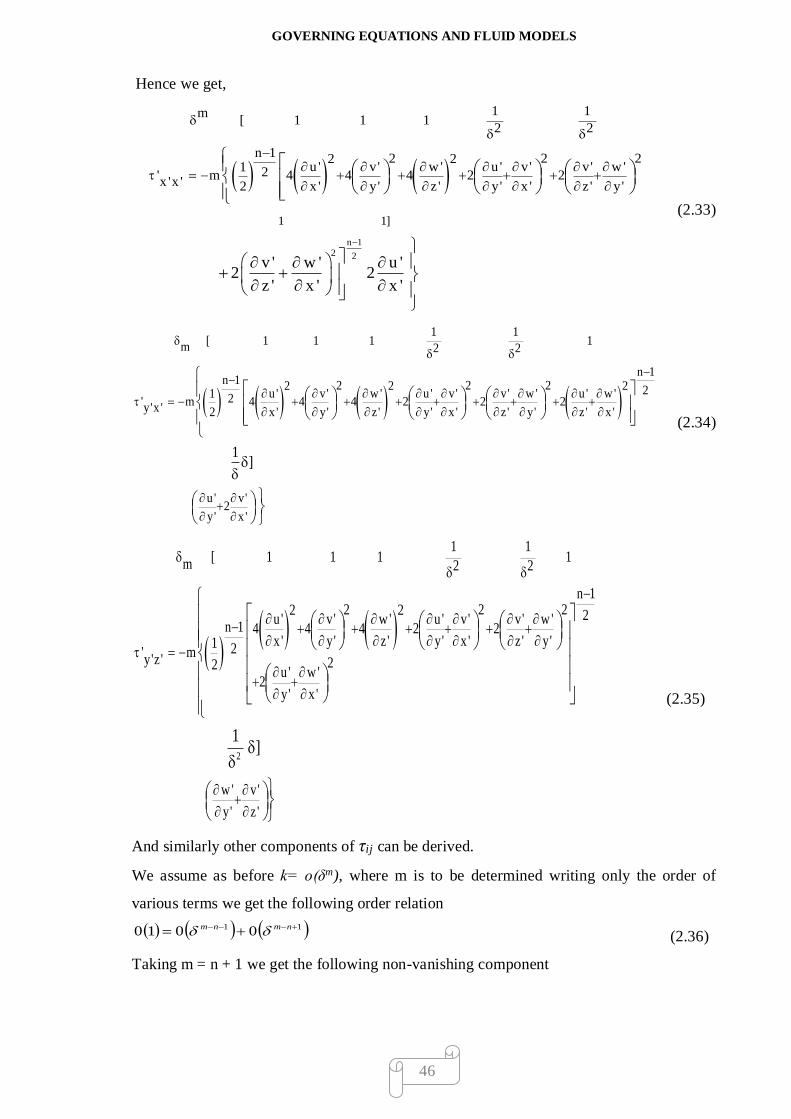
GOVERNING EQUATIONS AND FLUID MODELS
46
Hence we get,
n 12 2
1 1]
1 1m[ 1 1 1
2 2
n 1 2 2 22 2u ' v' w ' u ' v' v' w '1 2' m 4 4 4 2 2
x 'x ' 2 x ' y' z ' y' x ' z ' y '
v ' w ' u '2 2
z ' x ' x '
(2.33)
1 1[ 1 1 1 1
m 2 2
n 1n 1 2 2 22 2 2 2u ' v' w ' u ' v' v' w ' u ' w '1 2' m 4 4 4 2 2 2
y'x ' 2 x ' y' z ' y' x ' z ' y' z ' x '
u ' v'2
y' x '
1]
(2.34)
2
1 1[ 1 1 1 1
m 2 2
n 12 2 22 2 2u ' v' w ' u ' v' v' w '
n 1 4 4 4 2 2x ' y' z ' y' x ' z ' y'1 2' m
y'z ' 22u ' w '
2y' x '
w ' v'
y' z '
1]
(2.35)
And similarly other components of τij can be derived.
We assume as before k= o(δm), where m is to be determined writing only the order of
various terms we get the following order relation
11 0010 nmnm (2.36)
Taking m = n + 1 we get the following non-vanishing component

GOVERNING EQUATIONS AND FLUID MODELS
47
'
'
'
'2
'
'2
2
1'
2
122
2
1
''y
u
y
w
y
um
nn
xy
Or
'
'
'
'
'
''
2
1
22
''y
u
y
w
y
um
n
xy
(2.37)
Similarly, other non-vanishing components will be
'
'
'
'
'
''
2
1
22
''y
w
y
w
y
um
n
zy
(2.38)
Remaining shear-stress components vanish under the boundary-layer assumption. In a
similar way the stress-strain relationship for various visco-inelastic fluid models can be
derived.
Few fluid models which we have used are discussed below.
2.7.1 SISKO FLUID MODEL
So many real fluids are available which is follows the Sisko model of non-Newtonian
fluids proposed by Sisko. Polymeric suspensions such as waterborne coatings are known to
be non-Newtonian in nature and are follow the Sisko model. The viscosity of such coatings
depends on the shear rate and the strain history. An example that lends itself to such types
of coating is metallic automotive basecoat. Of course the most well know Sisko fluids are
lubricating greases. In fact most psueodplastic fluids, drilling fluids and cement slurries
without yield stress follow the Sisko model. For the Sisko fluid model shearing stress v/s
rate of strain is given by the relations (for 3-D flows).
12 2 2
' '
' ' ''
' ' '
n
y x
u w ua b
y y y
12 2 2
' '
' ' ''
' ' '
n
y z
u w wa b
y y y
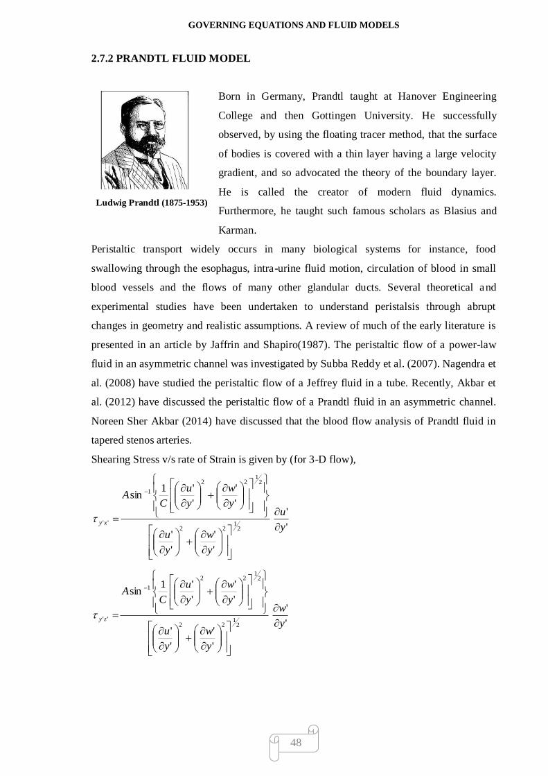
GOVERNING EQUATIONS AND FLUID MODELS
48
2.7.2 PRANDTL FLUID MODEL
Ludwig Prandtl (1875-1953)
Born in Germany, Prandtl taught at Hanover Engineering
College and then Gottingen University. He successfully
observed, by using the floating tracer method, that the surface
of bodies is covered with a thin layer having a large velocity
gradient, and so advocated the theory of the boundary layer.
He is called the creator of modern fluid dynamics.
Furthermore, he taught such famous scholars as Blasius and
Karman.
Peristaltic transport widely occurs in many biological systems for instance, food
swallowing through the esophagus, intra-urine fluid motion, circulation of blood in small
blood vessels and the flows of many other glandular ducts. Several theoretical and
experimental studies have been undertaken to understand peristalsis through abrupt
changes in geometry and realistic assumptions. A review of much of the early literature is
presented in an article by Jaffrin and Shapiro(1987). The peristaltic flow of a power-law
fluid in an asymmetric channel was investigated by Subba Reddy et al. (2007). Nagendra et
al. (2008) have studied the peristaltic flow of a Jeffrey fluid in a tube. Recently, Akbar et
al. (2012) have discussed the peristaltic flow of a Prandtl fluid in an asymmetric channel.
Noreen Sher Akbar (2014) have discussed that the blood flow analysis of Prandtl fluid in
tapered stenos arteries.
Shearing Stress v/s rate of Strain is given by (for 3-D flow),
'
'
'
'
'
'
'
'
'
'1sin
21
22
21
22
1
''y
u
y
w
y
u
y
w
y
u
CA
xy
'
'
'
'
'
'
'
'
'
'1sin
21
22
21
22
1
''y
w
y
w
y
u
y
w
y
u
CA
zy

GOVERNING EQUATIONS AND FLUID MODELS
49
2.7.3 PRANDTL – EYRING
Prandtl-Eyring model is an approximation of perfectly plastic fluids. Features of this model
are the behavior of lubricant.
Shearing Stress v/s Rate of Strain is given by(for 3-D flow),
'
'
'
'
'
'
'
'
'
'1sinh
21
22
21
22
1
''y
u
y
w
y
u
y
w
y
u
BA
xy
'
'
'
'
'
'
'
'
'
'1sinh
21
22
21
22
1
''y
w
y
w
y
u
y
w
y
u
BA
zy
2.7.4 WILLIAMSON FLUID MODEL
William Froude (1810-79)
He born in England and engaged in shipbuilding. In his sixties
started the study of ship resistance, building a boat testing pool
(approximately 75m long) near his home. After his death, this
study was continued by his son, Robert Edmund Froude (1846-
1924). For similarity under conditions of inertial and
gravitational forces, the non dimensional number used carries
his name.
Williamson fluid is characterized as a non-Newtonian fluid with shear thinning property
i.e., viscosity decreases with increasing rate of shear stress. Chyme in small intestine is
assumed to behave like Williamson fluid. Peristaltic motion is one of the most
characteristics fluid transport mechanism in many biological systems. It pumps the fluids
against pressure rise. Williamson (1929) discussed the flow of pseudo plastic materials and
proposed a model equation to describe the flow of pseudo plastic fluids and experimentally
verified the results. Lyubimov and Perminov (2002) discussed the flow of a thin layer of a
Williamson fluid over an inclined surface in the presence of a gravitational field. Cramer et
al. (1968) showed that this model fits the experimental data of polymer solutions and

GOVERNING EQUATIONS AND FLUID MODELS
50
particle suspensions better than other models. In the Williamson fluid model, both the
maximum viscosities (μ∞) and minimum viscosities (μ0) are considered. So, for pseudo
plastic fluids (for which the apparent viscosity does not go to zero at infinity), it will give
better results.
Shearing Stress v/s rate of Strain is given by(for 3-D flow),
'
'
'
'
'
'
'
'
21
22''
y
u
y
w
y
uB
y
uA
xy
'
'
'
'
'
'
'
'
21
22''
y
w
y
w
y
uB
y
wA
zy

CHAPTER-3
SIMILARITY ANALISIS AND NUMERICAL
METHODS
3.1 SIMILARITY ANALYSIS
An exigent problem faced by engineers and applied mathematicians are working in a field
of study is to find exact solutions of the basic equations arising in that field while
employing a minimum number of simplifying assumptions. In number of cases, the basic
equations of any fluid expressing the physical laws are partial differential equations.
Ideally, one hopes to find exact solution of these equations. In certain instances standard
methods of solution (separation of variables, Laplace transforms etc…) are of value and
solutions can be found. Nevertheless, there are numbers of problems available for which
the solution can’t found by the usual classical methods. This is particularly true if the
equations encountered are nonlinear. An excellent example of a nonlinear system of
equations which presents formidable obstacles to classical analysis is the system of
equations of motion for a viscous fluid flow.
We are interested to find the solution of such sets of partial differential equations for
applied fields. But for the solution of such partial differential equation common classical
methods failed to yield result. So we have to apply transformations that are reduced the
system of partial differential equations into system of ordinary differential equations.
These solutions are known as similarity solutions.
In similarity analysis method, we find the transformation between independent and
dependent variables appeared in the given fluid flow equations in such a way that the
numbers of independent variables are at least one less than in the transformed differential
equation compared to the original partial differential equation. For instance if a given
partial differential equation contains two independent variables then after applying
similarity transformation it is transformed into an ordinary differential equation (i.e.
equation having one independent variable). Due to this fact, the major application of

SIMILARITY ANALISIS AND NUMERICAL METHODS
52
similarity transformations has been used to reduction of certain classes of non-linear partial
differential equations in to ordinary differential equations. Blasius (1908) gives model
example for similarity analysis method. He converted the system of nonlinear partial
differential equations for flow over a flat plate into only one ordinary differential equation.
In recent times it is more demanded and increase interest to find the necessary and
sufficient conditions for the existence of similarity solutions. Also find the general solution
method for similarity solutions of various classes of non linear partial differential
equations. From the literature review there are four similarity analysis methods. Which are
as follows :
(a) Group theoretic
(b) Separation of variables
(c) Free Parameter
(d) Dimensional Analysis
We have applied group theoretic method for our problems which is discussed below.
3.1.1 GROUP THEORETIC METHOD
Mathematically, Group theory method is the most difficult approach for finding similarity
transformation. This concept will eventually lead to more general developments of
similarity analysis. For better understanding of this concept we will consider one simple
application.
According to this method we can reduce a system of partial differential equations having
two independent variables into a system of ordinary differential equations having one
independent variable. For that we can find a relation between new independent variable η
and old independent variables x and y in such way that which is absolutely invariant under
a taken group transformation. As well as we can find a relation between the dependent
variables that is also an absolute invariant under a taken group transformation.
Let’s consider the basic equations for laminar boundary–layer flow of Newtonian fluid
over a flat plate (M. Patel, 2007).
2
2
u u uu v
x y y
(3.1)

SIMILARITY ANALISIS AND NUMERICAL METHODS
53
0
y
v
x
u
(3.2)
Where, = Kinematic viscosity
With the boundary conditions are:
0 0 0u and v at y (3.2a)
0u U at y (3.2b)
Take one-parameter linear group transformation of variables x, y, u and v as
:
n
m
p
q
x a x
y a yG
u a u
v a v
(3.3)
Where, a = one parameter group transformation constant.
We need to determine the values of constants n, m, p and q in such way that given partial
differential equations are invariant under taken group transformation. For this we substitute
expressions from equation (3.3) in equations (3.1) and (3.2) we have,
22 2
2
m k n m l m lu u ua u a v a
x y y (3.4a)
0
m k n lu va a
x y
(3.4b)
For finding the invariance it is necessary to choose the power of “a” in such manner that
the transformed equations look exactly the same in terms of the new variables as they did
with the old. We need only to equate these exponents and cancel out the common powers
of a.
Equating powers of a in equations (3.4a) and (3.4b) we get the following system of
equations,
2 2 m k n m l m l (3.5)
m k n l (3.6)
From the set of equations (3.5) and (3.6) we get relation between constants,
2 n l and m k l (3.7)
Now we define new independent variable η using previous independent variables x and y
which is absolute invariant under the taken group transformation.

SIMILARITY ANALISIS AND NUMERICAL METHODS
54
sy x
(3.8)
The invariance of is satisfied by
snmss xayaxyyx (3.9)
We get,
nms
(3.10)
Also, we define new dependent variables using previous variables in such a way that they
are absolute invariant under the taken group transformation.
1
rf u x (3.11)
2
tf v x (3.12)
The invariance dependent variables f1 and f2 satisfies,
2( )( )r r k l k ru x u x a u a x (3.13)
( v)( )t t l k tv x v x a a x (3.14)
Equating powers of constant a on both the sides of equations (3.13) and (3.14) we get,
2 0k l kr (3.15)
0l kt (3.16)
Finally, from the equation (3.15) the value of r and from the equation (3.16) the value of t
is substitute in equation (3.11) and (3.12) respectively.
2 21 1
1 1
l lr k kf ux ux or u x f
(3.17)
2 2
l lt k kf vx vx or v x f
(3.18)
It is now possible to substitute these expressions for u and v in the original set of equations
(3.1) and (3.2) we have ordinary differential equations in new dependent variables f 1 and
f2.
The continuity equation (3.2) is reduced as,

SIMILARITY ANALISIS AND NUMERICAL METHODS
55
22 1 ' '
1 1 2
21 0
ll lkk k
u v lx f x f x f
x y k x y
(3.19)
Now,
1llkk
l ly x y x
x x k k x
(3.20)
lkx
y
(3.21)
Equation (3.19) becomes,
2 2 2' '
1 1 2
21 0
l l lk k k
l lx f x f x f
k k
(3.22)
Variable x 0 so we have,
' '
1 1 2
21 0
l lf f f
k k
(3.23)
Now let’s choose 12
lk to simplify our expression in equation (3.23) we obtain,
'
' 1
22
ff
(3.24)
We substitute our expressions for u and v from equation (3.17) and (3.18) respectively into
the equation (3.2) with the choosing 2
1n
m we get,
'1 1
' ' ' 11 1 2 22 1 1
2
f fx f f x f x
x
(3.25)
Again for x 0 we have
'
' ' '1 1
2 1 12
f ff f f (3.26)
Thus we have two ordinary differential equations (3.24) and (3.26) for the functions f1 and
f 2. The results can be put in more conventional form by letting 1f F
Then the form of equation (3.24)
2
".
2
1' .
2
Ff d const
F F const
(3.27)
Taking integration constant zero and substitute the value of f2 from equation (3.27) in
equation (3.26) we get

SIMILARITY ANALISIS AND NUMERICAL METHODS
56
1 ' "
' "2 2
F FF F F F
It is also written as,
"0
2
FFF (3.28)
Finally, equation (3.28) is similarity equation for defined flow problem. The major
approaches to finding similarity transformations have been outlined up to this point. In this
method we combined two methods Group transformation method for reduction of
independent variables and separation of variables method for combined system of
equations into a single equation. So together both the methods are called “dimensional
analysis method” can be established as being a special group theoretical method.
3.1.2 FREE PARAMETER METHOD
The free parameter method is also one of the types of similarity analysis method. Using
this method we reduce the number of independent variables as well as we find proper
transformation of the boundary values. The choice of transformation is determined by the
boundary values of the original problem and takes transformation of dependent variables in
such way that the boundary values of defined flow problem is transformed into meaningful
boundary values in terms of the new set of dependent variables.
The particular procedure is perhaps best illustrated by example. In this example we also
point out one of the basic weakness in the use of the free parameter type of analysis.
Consider a classical flow over a flat plate. We denote u by the velocity of the flow within
the boundary layer in the direction of flow (along x-axis) and v is the velocity in the
boundary layer normal to the flow(along y-axis). The velocity of the fluid is equal to zero
on the surface of the plate and varies from zero to the “mainstream” velocity U0 in a very
thin region near the surface of the plate called the boundary layer. The flow equations for
defined flow problem are given by equations (3.1) and (3.2).
First we eliminate one of the dependent variables u or v from the equation (3.2).
From equation (3.1) velocity component v given by,
0
yu
v dyx
(3.29)

SIMILARITY ANALISIS AND NUMERICAL METHODS
57
Substitute value of equation (3.29) in equation (3.2),
2
2
0
yu u u u
u dyx y x y
(3.30)
Now our goal is to convert equation (3.30) into single independent variable η. Also we
express u as a function of η in such a way that the boundary conditions equations (3.2a)
and (3.2b) which have been specified for the original equation carry over into meaningful
boundary conditions in the transformed equation.
For this take 0
u
Ube a function of independent variable η as,
0
'u
fU
(3.31)
With Boundary conditions;
0
0
' 0u
f atU
(3.32)
0
' 1u
f atU
(3.33)
Where,
0 0, , ,y x
Substitute the value of equation (3.31) in equation (3.30) we get,
2 2
2
00
' " ' " "
y
F F F dy F F Fx x y U y y
(3.34)
Now assume that
g xy
(3.35)
So equation (3.34) will reduce as
0
3" 0
U dgF F F
dxg
(3.36)
The problem of reducing equation (3.36) to an ordinary differential equation in η reduces
to merely choosing.
0
3
1tan
2
U dgcons t
dyg (3.37)
Together equation (3.36) and (3.37) we get,

SIMILARITY ANALISIS AND NUMERICAL METHODS
58
1" 0
2F FF (3.38)
With boundary conditions:
lim
0 ' 0 0 ' 1f f and f
(3.39)
Equation (3.38) called the Blasius equation.
In this method we specifies an acceptable form for the new dependent variables but it does
not give any conditions on the transformed independent variables which is the chief
weakness of this method. The proper form for the independent, however, ultimately is
chosen. Group theory method is better to apply.
3.2 QUASILINEARIZATION METHOD
The quasi linearization approach is a generalized Newton-Raphson technique for
functional equations. It is converges quadratically to the exact solution if there is
convergence and it has monotone convergence.
Let us consider the nonlinear second order differential equation as follows:
''( ) ( '( ), ( ), )y x y x y x x (3.40)
With the boundary conditions
0 0( ) ( ) ,y a a and y b b a x b
(3.41)
The function can now be expanded about 𝑦0 (𝑥) by using the Taylor’s series expansion.
After neglecting second and higher order terms we have,
'0 ,0
'0 ,0
0 0 0
( , )
0
( , )
( '(x), ( ), ) ( '( ), ( ), ) ( ( ) ( ))
( '( ) '( ))'
y y x
y y x
y y x x y x y x x y x y xy
y x y xy
(3.42)
From equation (3.40) and (3.42) we have,
'0 ,0
'0 ,0
0 0 0
( , )
0
( , )
''( ) ( '( ), ( ), ) ( ( ) ( ))
( '( ) '( ))'
y y x
y y x
y x y x y x x y x y xy
y x y xy
(3.43)
Solving equation (3.43) for ( )y x and say it1( )y x .

SIMILARITY ANALISIS AND NUMERICAL METHODS
59
Therefore, equation (3.43) can be written as,
' '0 , 0 ,0 0
1 0 0 1 0 1 0
( , ) ( , )
''( ) ( '( ), ( ), ) ( ( ) ( )) ( '( ) '( ))'
y y x y y x
y x y x y x x y x y x y x y xy y
Similarly, above equation expanded about y1(x) we have,
' '1, 1,1 1
2 1 1 2 1 2 1 '
1 1( , ) ( , )
''( ) ( '( ), ( ), ) ( ( ) ( )) ( '( ) '( ))
y y x y y x
y x y x y x x y x y x y x y xy y
Continue the procedure up to desired accuracy. We have recurrence relation as,
',
',
1 1
( , )
1
( , )
''( ) ( '( ), ( ), ) ( ( ) ( ))
( '( ) '( ))'
r r
r r
r r r r r
r y y x
r r
r y y x
y x y x y x x y x y xy
y x y xy
(3.44)
Where, r = 0, 1, 2, 3…
Where, 𝑦r (𝑥) is known and using it we can obtain 𝑦r+1 (𝑥). Equation (3.44) is always a
linear differential equation and boundary conditions are:
1 0 1 0( ) ( ) ,r ry a a and y b b a x b
Similarly, one can follow the same procedure for higher order nonlinear differential
equations to obtain the recurrence relation
1 '
1
11 '
1
0
( ) ( ( ),....., y ( ), ( ), )
( ( ) ( )) ( ( ),....., y ( ), ( ), )i
n n
r r r r
ni i n
r r r r ryi
L y x y x x y x x
y x y x y x x y x x
(3.45)
Where, 𝑛 is the order of the differential equation. Equation (3.45) is always a linear
differential equation and can be solved recursively.
3.2 NUMERICAL METHOD: FINITE DIFFERENCE METHOD
The solution of Ordinary Differential Equations (ODEs) is found by two ways first is
discrete method and second is numerical method. Discrete methods are one of the oldest
and most successful areas of numerical calculation. One of the examples to need for such
calculation is the problem of predicting the motions of planets or other bodies in the space.
The governing differential equations for the sun and the planet are known and Newton

SIMILARITY ANALISIS AND NUMERICAL METHODS
60
showed that how to solve it exactly. In the last three centuries no one has ever found its
exact solution in the case of more than two bodies. So, the numerical calculation of such
orbits is effortless by modern standards.
The most popular families of numerical methods for solution of ODEs are:
Finite Difference Method
Finite Element Method
Range -Kutta Method
For finding the solution of two ending point boundary value problem using finite
difference method, we replace the derivatives occurring in the differential equation as well
as in the boundary conditions by means of their finite difference approximations. By
Substituting finite difference we obtain sets of linear equation and it is solve by any
standard procedure.
Now procedure to find the appropriate finite difference (central difference) approximation
of the derivatives as follows.
The Taylor’s series expansion of (x h)f
2 3
( ) ( ) '( ) ''(x) '''(x) ......2 6
h hf x h f x hf x f f
For which we obtain,
2( ) ( )'( ) ''( ) '''(x) ......
2 6
f x h f x h hf x f x f
h
( ) ( )'( ) ( )
f x h f xf x O h
h
, (3.46)
Equation (3.46) is called the forward difference approximation formula for '( )f x
Similarly, by taking Taylor’s series expansion for (x h),f
2 3
( ) ( ) '( ) ''( ) '''( ) ......2 6
h hf x h f x hf x f x f x
Neglecting second and higher order terms we obtain,
( ) ( )'( ) ( )
f x f x hf x O h
h
, (3.47)
Equation (3.47) is called the backward difference approximation formula for '( )f x .

SIMILARITY ANALISIS AND NUMERICAL METHODS
61
A central difference approximation formula for '( )f x is given by taking addition of
equations (3.46) and (3.47) we have,
( ) ( )'( ) ( )
2
f x h f x hf x O h
h
(3.48)
It is clear that it gives better approximation for '( )f x than the forward and backward
difference approximation.
Again adding for ''( ),f x
'''( )f x we have,
2
2
( ) 2 ( ) ( )''( ) ( )
f x h f x f x hf x O h
h
(3.49)
3
3
( 2 ) 2 ( ) 2 ( ) ( 2 )'''( ) ( )
2
f x h f x h f x h f x hf x O h
h
(3.50)
In similar manner, it is possible to derive the central finite difference approximations
formula for higher order derivatives to solve boundary value problems.
We divide the range [x0, xn] into n equal subintervals of width h.
So that the value of x at ith node is given by,
0 , 1,2,3,....., nix x ih i
And their corresponding values of f (x), '( ), ''( )f x f x and '''( )f x at ith node point is obtained
by,
0( ) ( ) , 1,2,3,....., ni if x f f x ih i
The values of at the ith node can now be written as,
1 1'( ) ( )2
i ii
f ff x O h
h
(3.51a)
21 1
2
2''( ) ( )i i i
i
f f ff x O h
h
(3.51b)
32 1 1 2
3
2 2'''( ) ( )
2
i i i ii
f f f ff x O h
h
(3.51c)
Equations (3.51a)-(3.51c) central difference formulas for derivatives are substituting in
ODE we have system of linear equations then it is solve by Finite Difference method with
boundary conditions we have solution. If we increase the number of subintervals we find
the solution up to desired accuracy.

CHAPTER-04
NUMERICAL SOLUTION OF BOUNDARY
LAYER EQUATION OF PRANDTL FLUID
FLOW
4.1 INTRODUCTION
The complex rheology of biological fluids has motivated investigations involving different
non-Newtonian fluids. In recent years, non-Newtonian fluids have become more and more
important industrially. Polymer solutions, polymer melts, blood, paints and slurries,
shampoo, toothpaste, clay coating and suspensions, grease, cosmetic products, custard, are
the most common examples of non-Newtonian fluids. Academic curiosity and practical
applications have generated considerable interest in finding the solutions of differential
equations governing the motion of non-Newtonian fluids. The property of these fluids is
that the stress tensor is related to the rate of deformation tensor by some non-linear
relationship. These fluids present some interesting challenges to researchers in engineering,
applied mathematics and computer science. Thus wide usages of these fluids have
prompted modern researchers to explore extensively; the fields of non-Newtonian fluids.
The similarity solutions play an important role in investigating the non-Newtonian effects
especially in the boundary layer flows. Under the requirements of both academic as well as
practical application to find the similarity solution of differential equation of fluid (Non-
Newtonian) motion. In addition to the fact that it is the only class of exact solutions for the
governing differential equations it serves also as a reference to check the approximate
solutions. However, these solutions have limitations in cases of boundary layer flows as it
exists for the limit case of velocities at the edge of the similarity analysis.

NUMERICAL SOLUTION OF BOUNDARY LAYER EQUATION OF PRANDTL FLUID FLOW
63
4.2 HISTORICAL REVIEW
In 1969, Moran et al. (1968) have explained similarity analysis in very systematic way to
convert given system of partial differential equations in to a system of ordinary differential
equations.
Abd-el-Malek et al. (2002), Parmar and Timol (2011), Adnan et al. (2011), Darji and
Timol (2013) and Jain and Timol (2015) have applied deductive group transformation
method for various types of fluid flow problems.
Very rare information is available in literature about the Prandtl fluid model. Recently,
many researchers discussed about the peristaltic transport of Prandtl fluid.Akbar et al.
(2012) examined the Prandtl fluid model in an asymmetric channel. Sucharitha et al.
(2012) and Navaneeswara et al. (2012) discussed the conducting Prandtl fluid in a porous
channel. Jothia et al. (2012) further explained the peristaltic transport of same model under
the effects of magnetic field. The flow equations for the Prandtl fluid model are developed
in both a fixed and moving frame of references by Nadeem et al. (2014).N Akbar et al.
(2014) Have been discussed the blood flow analysis of Prandtl fluid model in tapered
stenosed arteries. The governing equations for considered model are presented in
cylindrical coordinates. Perturbation solutions are constructed for the velocity, impedance
resistance, wall shear stress and shearing stress at the stenosis throat. The effects of
magnetohydrodynamic (MHD) on peristaltic transport of Prandtl fluid in a symmetric
channel have been studied under the assumptions of long wave length and low-Reynolds
number by A. Alsaedia et al. (2013). S. Jothia et al.(2012) have been studied the MHD
peristaltic flow of a Prandtl fluid in a uniform channel under the assumptions of long
wavelength and low Reynolds number. Series solutions of axial velocity and pressure
gradient are given by using regular perturbation technique when Prandtl number is small.
P. Gangavathi et al. (2014) have been discussed the effect of magnetic field on the
peristaltic flow of a Prandtl fluid in an asymmetric channel under the assumptions of long
wavelength and low Reynolds number.
Mathematically, the empirical relation for the Prandtl fluids Model is written M. Patel et al
(2013).
C
eA 1sin

NUMERICAL SOLUTION OF BOUNDARY LAYER EQUATION OF PRANDTL FLUID FLOW
64
Where, A and C are the material constants of the fluid. A possible generalization is
ij
mllm
ml
mllm
ml
ij e
ee
C
eeA
2
1
3
1
3
1
2
1
2
3
1
3
1
1
2
2sin
Where, τ and e are the stress tensor and the rate of deformation tensor respectively; A and
C are the Prandtl fluid parameter; m and l are fluid index.
4.3 PRESENT INVESTIGATION
This chapter develops to find the numerical solution of two-dimensional boundary layer
equations for Prandtl fluid model which is non-Newtonian fluid model and characterized
by the property that their components of deviatory stress is related to the rate of strain
tensor component by an arbitrary continuous function. Flow past on flat plate as well as
moving plate is discussed.
The similarity analysis is made of two-dimensional boundary layer equations for the flows
of purely viscous, steady and non-Newtonian fluids along with boundary conditions flat
plate as well as moving plat for similarity solutions. This flow equation is highly non-
linear PDE so it is very difficult to find its exact solution. Hence we try to find its
numerical solution in this chapter. The governing non-linear partial differential equations
of the laminar boundary layer flow of non-Newtonian fluid are transformed into non-linear
ordinary differential equations using one parameter group transformation method. Again
given ODE is also highly non-linear so we converted into linear ODE by quasi-
linearization method and find its numerical solution by Finite difference method &
graphical presentation using MATLAB solver.
4.4 GOVERNING EQUATIONS:(FOR THE FLOW PAST FLAT
PLATE)
The two dimensional laminar boundary layer flows past a semi-infinite flat surface is
considered. The geometry of present flow problem is shown in Figure 4.1. The governing
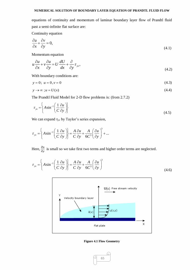
NUMERICAL SOLUTION OF BOUNDARY LAYER EQUATION OF PRANDTL FLUID FLOW
65
equations of continuity and momentum of laminar boundary layer flow of Prandtl fluid
past a semi-infinite flat surface are:
Continuity equation
0,u v
x y
(4.1)
Momentum equation
,yx
u u dUu v U
x y dx y
(4.2)
With boundary conditions are:
0; 0, 0y u v (4.3)
; ( )y u U x (4.4)
The Prandtl Fluid Model for 2-D flow problems is: (from 2.7.2)
1 1sinyx
uA
C y
(4.5)
We can expand τyx by Taylor’s series expansion,
3
1
3
1sin ...
6
yx
u A u A uA
C y C y C y
Here, 𝜕𝑢
𝜕𝑦 is small so we take first two terms and higher order terms are neglected.
3
1
3
1sin
6
yx
u A u A uA
C y C y C y
(4.6)
Figure 4.1 Flow Geometry

NUMERICAL SOLUTION OF BOUNDARY LAYER EQUATION OF PRANDTL FLUID FLOW
66
Now, introducing the stream function ψ (x, y)
andu vy x
(4.7)
Stream function in equation (4.7) satisfies the continuity equation (4.1). Substitute the
value of equation (4.7) and equation (4.6) in the momentum equation (4.2) and in the
boundary conditions.
22 2 3 2 3
2 3 3 2 32
dU A AU
y x y x y dx C y C y y
(4.8)
Boundary conditions are:
0 ; 0yy x
(4.9)
( ) ;U x yy
(4.10)
4.5 SIMILARITY SOLUTION : USING ONE PARAMETER
DEDUCTIVEGROUP THEORY METHOD
To obtain the similarity deductive solutions of the equations (4.8) under the boundary
condition (4.9) to (4.10), we apply one-parameter group method. After applied this method,
two independent variables x, y transforms into one independent variable η.
The group G of a class of one-parameter is taken of the form,
: ( ) ( )s sG S h a s k a (4.11)
Where, S stands for , , , , s sx y U h and k are real valued and differentiable in their real
argument a.
( ) ( )
( ) ( ):
( ) ( )
( ) ( )
x x
y y
U U
x h a x k a
y h a y k aG
h a k a
U h a U k a
(4.12)
; ; , ; ,s s
i i ij iji i j
h hS S S S i y x j y x
h h h
(4.13)
Equation (4.8) is said to be invariantly transformed for some function M (a), whenever

NUMERICAL SOLUTION OF BOUNDARY LAYER EQUATION OF PRANDTL FLUID FLOW
67
22 2 3 2 3
2 3 3 2 3
22 2 3 2 3
2 3 3 2 3
2
( )2
dU A AU
y x y x dx Cy y C y y
dU A AM a U
y x y x dx Cy y C y y
(4.14)
Substituting (4.12) and (4.13) in (4.14).We have,
2 2 2 2 3
2 2 2 3 3
23 2 3
3 7 2 3
22 2 3 2 3
2 3 3 2 3
( )
2
( )2
UU U
y x y x x y
y
h h h dU A hh U k
y x y x dx Ch h h h y h h y
A h
C h y y
dU A AM a U
y x y x dx Cy y C y y
(4.15)
From equation (4.15).We have the relation,
2 2 2 3
2 2 3 7( ) , 0
U U U
y x y x x y y x
h h h h h k hM a
h h h h h h h h
(4.16)
In a similar manner, the boundary conditions in equation (4.9) and (4.10) also being
invariant so from the equation (4.9) and (4.10) we have relations,
0,y U U
y
hK K h
h
(4.17)
Solving equation (4.16) and (4.17),
2 3, ,y x y U yh h h h h h (4.18)
Which is convert the group G of the form
3
2:
y x
y
y
y
x h x k
y h yG
h k
U h U
(4.19)
The above group G transforms the equations (4.8)-(4.10) invariantly.
If η = η(x,y) is the absolute invariant of the independent variables, then the absolute
invariant of the dependent variables is
( , ; , ) [ ( , )]; 1,2.j jg x y U x y j (4.20)
The basic theorem in group theory states that: a function g(x,y,ψ,U) is an absolute invariant
of a one parameter if it satisfies the following first-order linear differential equation.

NUMERICAL SOLUTION OF BOUNDARY LAYER EQUATION OF PRANDTL FLUID FLOW
68
4
1
0; , , ,i i i i
i i
gS S x y U
S
(4.21)
Where,
0 0( ), ( ); 1,2,3,4i is s
i i
h ka a i
a a
(4.22)
And a0 is the identity element of the group G.
Using equations (4.16) and (4.17) and equation (4.22), we have the following values of 𝛼 ′s
and 𝛽′𝑠,
312 4 2 4; 0
3 2
(4.23)
From the equation (4.21),
1 1 2 2 3 3 4 4 0g g g g
x y Ux y U
(4.24)
The absolute invariants of the independent variable η and dependent variables U and ψ are
determined using equation. (4.24) and (4.23) as,
13
1 1
233
1 1
1
13
1 1
( )
( ) ( )2
( )
y
x
x f
U x
(4.25)
Using the absolute invariants given in equation (4.25) in equations (4.8)-(4.10) we
obtained the non linear ordinary differential equations along with boundary conditions as
below:
2 2
3
3 32 1 0
2
A Af f f f f f
C C
(4.26)
With Boundary Conditions:
'(0) (0) 0 f f (4.27)
( ) 1 f (4.28)
Now for the solution of equation (4.26) under the boundary conditions (4.27)-(4.28) first
we convert quasi linearization method into linear ordinary differential equation, as

NUMERICAL SOLUTION OF BOUNDARY LAYER EQUATION OF PRANDTL FLUID FLOW
69
22
3
1 1
1 13
1
3 3' ( ) 2 ( ) ''( ) '''( ) ''( ) '''( ) 1
2
2 ''( )[ ( ) ( )] 2 '( )[ '( ) '( )]
32 ( )[ ''( ) ''( )] '''( )2 ''( )[ ''( ) ''( )]
2
3 3[ '''( ) '''( )]
n n n n n n
n n n n n n
n n n n n n n
n n
A Af f f f f f
C C
f f f f f f
Af f f f f f f
C
Af f
C
2
13''( ) [ '''( ) '''( )] 0
2n n n
Af f f
C
Simplifying above equation we have,
2
1 1 1
1 13
' 1 2 ''( ) ( ) 2 '( ) '( ) 2 ( ) ''( )
3 32 ( ) ''( ) '''( ) ''( ) ''( ) '''( ) 0
n n n n n n n
n n n n n n
f f f f f f f
A Af f f f f f
CC
(4.29)
To fit the curve, consider the solution
2
0 1 2nf A A A
(4.30)
Under the boundary conditions in (4.27) and (4.28) we get the values of constants,
0 1 20.5, 0, 0A A A
So equation (4.30) can be written as,
20.5nf (4.31a)
'
nf (4.31b)
' ' 1nf (4.31c)
' ' ' 0nf
(4.31d)
Substitute the values of equations (4.31a)–(4.31c) in equation (4.29) we get,
' ' ' 2 ' ' '
1 1 1 1
32 f 2 1n n n n
Af f f
C (4.32)
4.6 NUMERICAL SOLUTION : FINITE DIFFERENCE METHOD
Here the equation (4.32) is linear ordinary differential equation now we will find its
numerical solution using Finite difference method, Substitute the values of equations
(3.51a)–(3.51c) in equation (4.32). So at the ith node we get, the system of linear equations,

NUMERICAL SOLUTION OF BOUNDARY LAYER EQUATION OF PRANDTL FLUID FLOW
70
2 2 2 2
2 1 1
2 3 3
2
3 6 6[ 2 2 ] [ 2 2 ]
3[ 4 4 ] 2
i i i
i i
A A Af h h f h h f
C C C
Ah h f f h
C
(4.33)
This system of linear equations we solve it using MATLAB solver by dividing the interval
[0,1] into 1000 subintervals having equal length of each subintervals h=0.001. Given
numerical solution is presented graphically as below.
4.7 GRAPHICAL PRESENTATION
Figure 4.2 Stream function vs. Eta for different values of A
0 0.1 0.2 0.3 0.4 0.5 0.6 0.7 0.8 0.9 10
0.1
0.2
0.3
0.4
0.5
0.6
0.7
eta
str
eam
function
stream function vs. eta for C=0.5 and different A
A=3.5,C=0.5
A=2.5,C=0.5
A=1.5,C=0.5
A=C=0.5

NUMERICAL SOLUTION OF BOUNDARY LAYER EQUATION OF PRANDTL FLUID FLOW
71
Figure 4.3 Stream function vs. Eta for different values of C
Figure 4.4 Velocity profile vs. Eta for different values of A
0 0.1 0.2 0.3 0.4 0.5 0.6 0.7 0.8 0.9 10
0.1
0.2
0.3
0.4
0.5
0.6
0.7
0.8
0.9
eta
str
eam
function
streamfunction vs. eta for A=0.5 and different values of C
C=A=0.5 C=1. A=0.5 C=1.3,A=0.5 C=1.5,A=0.5
0 0.1 0.2 0.3 0.4 0.5 0.6 0.7 0.8 0.9 10
0.2
0.4
0.6
0.8
1
1.2
1.4
eta
f '
f ' vs. eta for C=0.5 and different values of A
A=C=0.5
A=1.5,C=0.5
A=2.5,C=0.5
A=3.5,C=0.5

NUMERICAL SOLUTION OF BOUNDARY LAYER EQUATION OF PRANDTL FLUID FLOW
72
Figure 4.5 Velocity profile vs. Eta for different values of C
4.8 RESULT AND DISCUSSION
Using one parameter deductive group method, the PDE of flow problems are transformed
into non linear ODE. Then non linear ODE is converted into linear ODE by quasi-
linearization method and then solved it using numerically finite difference method and
presented graphically by MATLAB solver. Figure 4.2 and Figure 4.3 gives the flow
pattern for various values of the Prandtl fluid parameter A and C respectively. Figure 4.4
and Figure 4.5 present the velocity profiles. Figure 4.4 represents the velocity profiles vs.
eta for different values of A and fix value of C=0.5. Figure 4.5 represents the velocity
profiles vs. eta for different values of C and fix value of A=0.5. For variable values of C,
the difference in increase in velocity is seems more clearly. Therefore from Figure 4.4 and
Figure 4.5, it conclude that the velocity profile increase more rapidly for different values
of C.
0 0.1 0.2 0.3 0.4 0.5 0.6 0.7 0.8 0.9 10
0.2
0.4
0.6
0.8
1
1.2
1.4
eta
f '
f ' vs. eta for A=0.5 and different values of C
A=0.5,C=0.5
C=1, A=0.5
C=1.5,A=0.5
C=1.3, A=0.5

NUMERICAL SOLUTION OF BOUNDARY LAYER EQUATION OF PRANDTL FLUID FLOW
73
4.9 GOVERNING EQUATIONS:(FOR THE FLOW PAST MOVING
PLATE)
The two dimensional laminar boundary layer flows past a semi-infinite moving surface is
considered. The governing equations of continuity and momentum of laminar boundary
layer flow of Prandtl fluid past a semi-infinite moving surface are:
Continuity equation
0,u v
x y
Momentum equation
,yx
u u dUu v U
x y dx y
With boundary conditions:
y=0: u=1, v=1 (4.34)
; 0y u (4.35)
For the Pradtl Fluid model stress tensor τ is taken from equation (4.5) and using one
parameter group theory method find it similarity equation we get momentum equation is
same as equation (4.26) and the boundary conditions as in equation (4.34) and (4.35) are
reduced as,
'(0) (0) 1 f f (4.36)
( ) 0 f (4.37)
Applying quasi linearization method to convert non linear differential equation (4.26) into
linear ordinary differential equation under the boundary condition equations (4.36)-(4.37)
as,
To fit the curve, consider the solution
2
0 1 2nf A A A (4.38)
Using boundary conditions in equations (4.36)-(4.37) we have constants,
A0 = - 0.499995, A1=1, A2 =1
So, equation (4.38) can be written as,
20.499995 1nf (4.39a)
' 0.99999 1nf (4.39b)
'' 0.99999nf (4.39c)
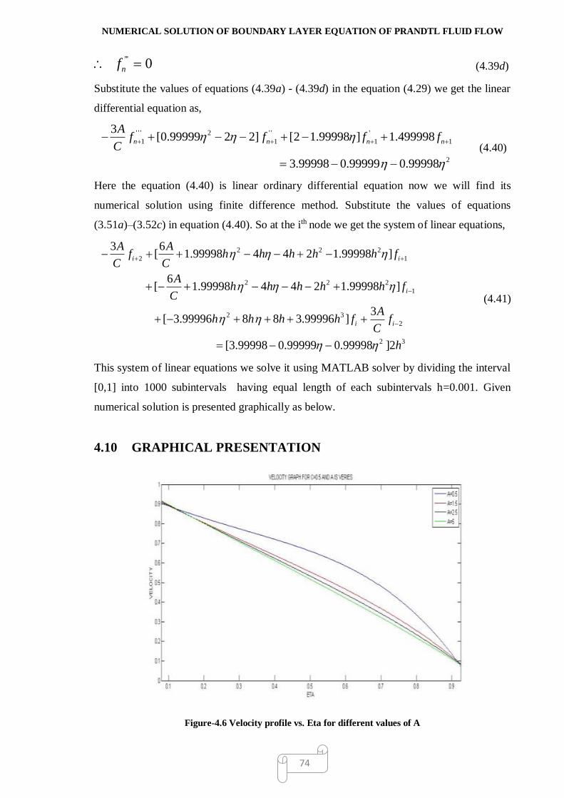
NUMERICAL SOLUTION OF BOUNDARY LAYER EQUATION OF PRANDTL FLUID FLOW
74
''' 0nf (4.39d)
Substitute the values of equations (4.39a) - (4.39d) in the equation (4.29) we get the linear
differential equation as,
' ' ' 2 ' ' '
1 1 1 1
2
3[0.99999 2 2] [2 1.99998 ] 1.499998
3.99998 0.99999 0.99998
n n n n
Af f f f
C
(4.40)
Here the equation (4.40) is linear ordinary differential equation now we will find its
numerical solution using finite difference method. Substitute the values of equations
(3.51a)–(3.52c) in equation (4.40). So at the ith node we get the system of linear equations,
2 2 2
2 1
2 2 2
1
2 3
2
2 3
3 6[ 1.99998 4 4 2 1.99998 ]
6[ 1.99998 4 4 2 1.99998 ]
3[ 3.99996 8 8 3.99996 ]
[3.99998 0.99999 0.99998 ]2
i i
i
i i
A Af h h h h h f
C C
Ah h h h h f
C
Ah h h h f f
C
h
(4.41)
This system of linear equations we solve it using MATLAB solver by dividing the interval
[0,1] into 1000 subintervals having equal length of each subintervals h=0.001. Given
numerical solution is presented graphically as below.
4.10 GRAPHICAL PRESENTATION
Figure-4.6 Velocity profile vs. Eta for different values of A

NUMERICAL SOLUTION OF BOUNDARY LAYER EQUATION OF PRANDTL FLUID FLOW
75
Figure 4.7 velocity profile vs. Eta for different values of C
4.11 RESULT AND DISCUSSION
Using one parameter group method, the PDE of flow problems are transformed into ODE.
The ODE are then solved numerically and presented graphically by MATLAB solver in the
present work. Figure 4.6 and Figure 4.7 present the velocity profiles. Figure 4.6
represents the velocity profiles vs. eta for different values of A and fix value of C=0.5.
Figure 4.7 represents the velocity profiles vs. eta for different values of C and fix value of
A=0.5. For variable values of C, the difference in increase in velocity is seems more
clearly. Therefore from Figure 4.6 and Figure 4.7, it conclude that the velocity profile
increase more rapidly for different values of C.
4.12 CONCLUSION
The methods for obtaining similarity transformations are devided into two categories (i)
Direct methods and (ii) group thoretic methods. The direct methods such as, seperation of
variables do not invoke group invarience. On the other hand, group theoretic methods are
more elegant mathematically. The main concept of invariance under a group of

NUMERICAL SOLUTION OF BOUNDARY LAYER EQUATION OF PRANDTL FLUID FLOW
76
transformation is invoked always . In the present paper, the governing non-linear partial
differential equations of the laminar boundary layer flow of non-newtonian fluid are
tranformed into non-linear ordinary differential equations using one parameter deductive
method. The Prandtl fluid model of non-Newtonian fluids is considered for the stress-strain
relationship.

CHAPTER-05
NUMERICL SOLUTION OF MHD BOUNDARY
LAYER EQUATIONS OF SISKO FLUID FLOW
5.1 INTRODUCTION
In practical applications and academic viewpoints it is most considerable interest to find
the solutions of governing partial differential equations of non-Newtonian fluids flow. In
non-Newtonian fluids the stress tensor and the rate of deformation tensor are always
related by some non-linear relationship. Some examples of non-Newtonian fluids are
shampoo, toothpaste, paint, clay coating and suspensions, grease, cosmetic products,
custard, blood and slurries etc… which obey this property of fluids. Due to great
commercial importance of such all the fluids it has been most considerable interest in non-
Newtonian fluids.
It is too difficult to exhibits all properties of non-Newtonian fluids by a single model and
also it cannot be described as simple like Newtonian fluids. Moreover, there has been
much confusion in the further classification of non-Newtonian fluids. The non-Newtonian
fluids are usually classified in three categories such as: (i) Fluids for which shear stress
depends only on the rate of shear (ii) Fluids for which relation between rate of strain and
shear stress depends on time (iii) Fluids for which the visco-inelastic fluids which possess
both viscous and elastic properties. Therefore the rate of shear and the shearing stress are
always very important for the mathematical structure of non-Newtonian fluids. But
deriving the mathematical formulation of such fluid model is really very difficult task.
5.2 HISTORICAL REVIEW
In past few decades, several researchers have analysed the problems of non-Newtonian
boundary layer flow of fluids past a different geometries. Bird et al. (1960), Hansen et al.
(1968), Kapur et al. (1982), Lee et al.(1966), Manisha et al. (2005,2008,2009,2010), Timol
et al. (1986,2004), Wells (1964)). Many fluids in the real world are non-Newtonian by

NUMERICL SOLUTION OF MHD BOUNDARY LAYER EQUATIONS OF SISKO FLUID
FLOW
78
nature. The study of such fluids is very much important due to their vast applications in the
field of engineering sciences and industries. Several fluid models of non-Newtonian fluid
have been investigated. A brief instruction and classification on various fluid models of
non-Newtonian fluid is given in detailed by Manisha et al.(2010,2013). Plenty of work
have been carried out by many scientist for Power-Law fluid model and Powell-Eyring
fluid model such as Djukic et al. (1973,1974),Na et al.(1967), Patel et
al.(2011,2012,2014,2009), Sirohi et al.(1984).
Very less information is available in literature about the fluid model proposed by Sisko
(1958). Na and Hansen (1967) have examined the flow of Sisko fluid between two circular
parallel disks. Bahraini et al. (1996) analysed the isothermal and axial laminar flow of
Power-law fluid and Sisko fluid in an annuli. The thin film flow problem of Sisko fluid and
Oldroyd fluid on a moving vertical belt was discussed nicely by Nemati et al. (2009).
Homotopy analysis method applied to solve the flow problem in their work. The flow
problem of Sisko fluid passing through an axisymmetric uniform tube was solved
analytically using the perturbation method and HAM by Nadeem et al.(2010). Moallemi et
al.(2011) have discussed the Homotopy perturbation method to solve the flow of a Sisko
fluid in pipe.
Recently, The numerical solution for the unsteady free convective flow of Sisko fluid past
flat plate moving through a binary mixture has been obtained by Olanrewaju et al. (2013).
Also, Siddiqui et al. (2013) has examined the drainage of Sisko fluid film down a vertical
belt. Asghar et al. (2014) have presented the equations for the peristaltic flow of MHD
Sisko fluid in a channel. They have considered the effect of strong and weak magnetic
fields both.
Mathematically, Stress tensor for Sisko Model can be written as,
1
1:
2
n
a b
(5.1)
Where, = stress tensor and = the rate of deformation tensor
a, b and n are constants and it is defined differently for different fluids.
Here we considered the problem of steady two dimensional MHD boundary layer flows of
non-Newtonian fluids. Sisko fluid model is considered for stress-strain relationship.

NUMERICL SOLUTION OF MHD BOUNDARY LAYER EQUATIONS OF SISKO FLUID
FLOW
79
Similarity and numerical solutions are obtained for the flow problem. All the cases are
presented with graph.
5.3 PRESENT INVESTIGATION
This chapter develops to find the numerical solution of two-dimensional boundary layer
equations for Sisko fluid model which is non-Newtonian fluid and characterized by the
property that their components of deviatory stress is related to the rate of strain tensor
component by an arbitrary continues function.
The similarity analysis is made of two-dimensional boundary layer equations for defined
flow is purely viscous, steady and non-Newtonian fluids and under the influence of
magnetic effect along with the boundary conditions for flat plat as well as in moving plat.
Resultant similarity equation of defined flow problems are highly non linear Partial
differential equations and so it is very difficult find its exact solution. Hence we try to find
its numerical solution in this chapter. The governing non-linear partial differential
equations of the laminar boundary layer flow of non-newtonian fluid are tranformed into
non-linear ordinary differential equations using one parameter group tranformation
method. Again given ordinary differential equation is also highly non linear so we
converted into linear ordinary differential equation by quasilinearisation method and find it
solution by Finite difference method and graphically presented by MATLAB solver.
5.4 GOVERNING EQUATION: (FOR THE FLOW PAST FLAT
PLATE)
In present problem flow considered in two dimensional spaces parallel to X-direction and
Y-axis is normal to it. The laminar MHD boundary layer flow of Sisko fluid past a semi-
infinite flat plate. The governing equations (continuity equation and momentum equation)
of defined fluid flow problem are:
Continuity equation
0,u v
x y
(5.2)
Momentum equation

NUMERICL SOLUTION OF MHD BOUNDARY LAYER EQUATIONS OF SISKO FLUID
FLOW
80
2
0 (U u)yx
u u dUu v U B
x y dx y
(5.3)
With boundary conditions
y=0: u=0, v=0 (5.4)
y : u=U(x) (5.5)
For the Sisko Fluid Model in 2-D flow problems stress tensor is given by equation (5.1).
So momentum equation (5.3) is converted into
1
2
0 (U u)
n
u u dU u uu v U a b B
x y dx y y y
(5.6)
5.5 SIMILARITY SOLUTION: USING ONE PARAMETER GROUP
THEORY METHOD
To obtain the similarity solutions of the continuity equation (5.2) and momentum equation
(5.6) under the boundary conditions (5.4) - (5.5) we take one-parameter scaling group
transformation as,
1
2
3
4
5
G:
y A y
x A x
u A u
v A v
U A U
(5.7)
Introducing equation (5.7) in equations (5.2), (5.6) and using simple chain rule formula we
get
3 2 4 1u vu vA A
x y x y

NUMERICL SOLUTION OF MHD BOUNDARY LAYER EQUATIONS OF SISKO FLUID
FLOW
81
23 2 4 3 1
( n 1) ( n 1) 22 2 3 1 15 2 3 1 35 3
12 2
2 2
12 2
2
02 2( )
n
n
u uu u dU u u uu v U a nb A u A v
x y dx y x yy y
d U u u uA U A a nbA B A U A u
d x yy y
Above set of equations remains invariant under taken group transformation G. So we have
relation between 𝛼 ′𝑠 as,
3 2 4 1
3 2 4 3 1 5 2 3 1 5 32 2 n (n 1)
Solving above set of equations we get relation between α’s as,
1 2 3 4 53 3 3 3
2
1
1put
3
3 4 5
Now we define new independent variable η of two independent variables x and y, is called
similarity independent variable and dependent variables f(η), g(η) and h(η) of u, v and U
respectively, are called similarity dependent variables Seshadri et al. (1985).
1
31̀
3
y y
x yx
x
(5.8)
1
3
' ( )u
f
x
(5.9)
1
3
( )v
g
x
(5.10)
11
3
( )U
h c
x
(5.11)
Substituting the values in equations (5.8)-(5.11) in equations (5.2) and (5.6) will transform
into the following equations:
' ( ) ( ) 3 '( ) 0f f g (5.12)
1
12 2
2
0 1
' ( ) ( ) ( ) 3 ( ) ( ) 3 ( ) 3 ( ) ( )
3 ( ( ))
nf f f g f c af nb f f
B c f
(5.13)

NUMERICL SOLUTION OF MHD BOUNDARY LAYER EQUATIONS OF SISKO FLUID
FLOW
82
Now solving equation (5.12) for g,
1
'( ) ''( ) '( )3
g f f
1
( ) ''( ) '( )3
g f f d
1
( ) '( ) 2 ( )3
g f f
Now, putting the value g in equation (5.13) we obtained,
12 2
1
2
0 1
' ( ) 2 ( ) ''( ) 3 '''( ) 3 ''( ) '''( )
3 ( '( )) 0
nf f f c af nb f f
B c f
(5.14)
And the boundary conditions in equation (5.3) and (5.4) are reduced as,
0 0, 0 0, 1f f f (5.15)
2
0 0 1 1,Put B M and C
12
0
' ( ) 2 ( ) ''( ) 3 '''( ) 3 ''( ) '''( )
3 (1 '( )) 1 0
nf f f af nb f f
M f
(5.16)
We have equation (5.16) is non linear ordinary differential equation. First we convert
equation (5.16) into linear ordinary differential equation by quasi linearization method as,
1' 2 ' ' ' ' ' ' ' ' ' ' '
0
' ' ' ' '
1 1
' ' ' ' ' ' ' ' '
0 1 1 1
' ' '
( ) 2 ( ) ( ) 3 ( ) 3 ( ) ( ) 3 (1 ( ))
1 2 ( )( ( ) ( )) 2 ( )( ( ) ( ))
3 ( ( ) ( )) 2 ( )( ( ) ( )) 3 ( )
3 ( ) 3 ( 1)
n
n n n n n n n
n n n n n n
n n n n n n
n
f f f af nb f f M f
f f f f f f
M f f f f f af
af n n b f
2' ' ' ' ' ' ' ' '
1 1
1' ' ' ' ' ' ' '
1 1
( ) ( ( ) ( )) ( )
3 ( ) ( ( ) ( )) 0
n
n n n n
n
n n n
f f f
nb f f f
Simplifying above equation we get,
2
0 1 1 0 1
1 1
2 1
1
1
1
' 3 1 2 ''( ) ( ) 2 '( ) '( ) 3 '( )
2 ( ) ''( ) 2 ( ) ''( ) 3 '''( ) 3 ( 1)
''( ) ''( ) '''( ) 3 ( 1) ''( ) '''( )
3 ''( ) '''( ) 0
n n n n n n
n n n n n
n n
n n n n n
n
n n
f M f f f f M f
f f f f af n n
b f f f n n b f f
nb f f
(5.17)
With boundary conditions:
' '0 0, 0 0, 1n n nf f f (5.18)

NUMERICL SOLUTION OF MHD BOUNDARY LAYER EQUATIONS OF SISKO FLUID
FLOW
83
To fit the curve, consider the solution,
2
0 1 2nf A A A (5.19)
Under the boundary conditions in equation (5.18) we have the constants,
0 1 20.5, 0, 0A A A
So, equation (5.19) can be written as, fn = 0.5 η2
2 ' '' '''0.5 , , 1, 0n n n nf f f f (5.20)
Substitute the values of equations (5.20) in equation (5.17) we get,
''' 2 '' '
1 1 0 1 1 0(3nb 3 ) (2 3 ) f 2 1 3n n n na f f M f M (5.21)
5.6 NUMERICAL SOLUTION : FINITE DIFFERENCE METHOD
Here the equation (5.21) is linear ordinary differential equation now we will find its
numerical solution using Finite difference method, Substitute the values of equations
(3.51a) – (3.51c) in equation (5.21) at the ith node we get the system of linear equations.
2 2 2
2 0 1
2 3 2 2 2
0 1
3
2 0
(3nb 3 ) ( 6 6 2 2 3 )
( 4 4 ) (6 6 2 2 3 )
( 3nb 3 ) (1 3 )2
i i
i i
i
a f nb a h h h M f
h h f nb a h h h M f
a f M h
(5.22)
Case I: Non- MHD Sisko fluid
If we take M0 =0 in equation (5.22), then it will reduced in the case of non- magneto
hydrodynamic Sisko fluid. Then the system of linear equations (5.22) will reduced in the
following equation (5.23) with the same boundary conditions given in equation (5.18).
2 2 2 3
2 1
2 2 3
1 2
(3nb 3 ) ( 6 6 2 2 )f ( 4 4 )
(6 6 2 2 ) (3nb 3 ) 2
i i i
i i
a f nb a h h h h f
nb a h h f a f h
(5.23)
Case II: MHD Power-Law fluid
If we take a=0, b=1 in equation (5.22), then it will give us magneto hydrodynamic Power-
Law fluid flow. And the system of linear equations in equation (5.22) will reduced in the
following equation (5.24) with the same boundary conditions given in equation (5.18).

NUMERICL SOLUTION OF MHD BOUNDARY LAYER EQUATIONS OF SISKO FLUID
FLOW
84
2 2 2 2 3
2 0 1
2 2 2 3
0 1 2 0
3n ( 6 2 2 3 )f ( 4 4 )
(6 2 2 3 ) 3n (1 3 )2
i i i
i i
f n h h h M h h f
n h h h M f f M h
(5.24)
Case III: Non-MHD Power-Law fluid
If we take a=0, b=1 and Mo = 0 in equation (5.22), then it will give us non magneto
hydrodynamic Power-Law fluid. And the system of linear equations in equation (5.22) will
reduced in the following equation (5.25) with the same boundary conditions given in
equation (5.18).
2 2 2 3
2 1
2 2 3
1 2 0
3n ( 6 2 2 ) ( 4 4 )
(6 2 2 ) 3n (1 3 )2
i i i
i i
f n h h f h h f
n h h f f M h
(5.25)
Case IV: MHD Newtonian fluid
If we take a=1, b=0, n=1 in equation (5.22), then it will give us magneto hydrodynamic
Newtonian fluid. And the system of linear equations in equation (5.22) will reduced in the
following equation (5.26) with the same boundary conditions given in equation (5.18),
2 2 2 2 3
2 0 1
2 2 2 3
0 1 2 0
3 ( 6 2 2 3 ) ( 4 4 )
(6 2 2 3 ) 3 (1 3 )2
i i i
i i
f h h h M f h h f
h h h M f f M h
(5.26)
Case V: non- MHD Newtonian fluid
If we take a=1, b=0, n=1 and Mo = 0 in equation (5.22), then it will give us non magneto
hydrodynamic Newtonian fluid. And the system of linear equations in equation (5.22) will
reduced in the following equation (5.27) with the same boundary conditions given in
equation (5.18).
2 2 2 3
2 1
2 2 3
1 2
3 ( 6 2 2 ) ( 4 4 )
(6 2 2 ) 3 2
i i i
i i
f h h f h h f
h h f f h
(5.27)
Which is system of linear equations we solve it in MATLAB by dividing [0,1] interval into
1000 subinterval having length h=0.001.solution is presented graphically.

NUMERICL SOLUTION OF MHD BOUNDARY LAYER EQUATIONS OF SISKO FLUID
FLOW
85
5.7 GRAPHICAL PRESENTATION
Figure 5.1 MHD Sisko fluid with a=b=0.5, n=0.5 and different values of Mo
Figure 5.2 MHD Sisko fluid with a=b=0.5, Mo = 4 and different values of n
0 0.05 0.1 0.15 0.2 0.25 0.3 0.35 0.4 0.45 0.50
0.1
0.2
0.3
0.4
0.5
0.6
0.7
eta
f'
Mo = 1 Mo = 2 Mo = 4 Mo = 6
0 0.05 0.1 0.15 0.2 0.25 0.3 0.35 0.4 0.45 0.50
0.05
0.1
0.15
0.2
0.25
0.3
0.35
0.4
0.45
0.5
eta
f'
n=0.5 n=1 n=1.5 n=2

NUMERICL SOLUTION OF MHD BOUNDARY LAYER EQUATIONS OF SISKO FLUID
FLOW
86
Figure 5.3 MHD Power-Law Fluid with a=0, b=1, n=0.5 and different values of Mo
Figure 5.4 MHD Power-Law fluid for a=0, b=1, Mo = 4 and different n
0 0.1 0.2 0.3 0.4 0.5 0.60
0.1
0.2
0.3
0.4
0.5
0.6
0.7
eta
f'
Mo = 1 Mo = 2 Mo =4 Mo = 6
0 0.05 0.1 0.15 0.2 0.25 0.3 0.35 0.4 0.450
0.05
0.1
0.15
0.2
0.25
0.3
0.35
0.4
0.45
0.5
eta
f'
n=0.5 n=1 n=1.5 n=2

NUMERICL SOLUTION OF MHD BOUNDARY LAYER EQUATIONS OF SISKO FLUID
FLOW
87
Figure 5.5 MHD Newtonian fluid with a=1, b=0, n=1 and different Mo
Figure 5.6 All fluid with and without Magneto field effect
0 0.05 0.1 0.15 0.2 0.25 0.3 0.35 0.4 0.450
0.05
0.1
0.15
0.2
0.25
0.3
0.35
0.4
0.45
0.5
eta
f'
Mo = 1 Mo = 2 Mo = 4 Mo = 6
0 0.05 0.1 0.15 0.2 0.25 0.30
0.05
0.1
0.15
0.2
0.25
0.3
0.35
eta
f'
MHD Sisko
non-MHD Sisko
MHD Power Law
non-MHD Power Law
MHD Newtonian
non-MHD Newtonian

NUMERICL SOLUTION OF MHD BOUNDARY LAYER EQUATIONS OF SISKO FLUID
FLOW
88
5.8 RESULT AND DISCUSSION
The similarity solutions obtained for the defined flow problem are solved numerically and
presented graphically. Figure 5.1 and Figure 5.2 represent the velocity profile f ’ verses
eta. of laminar magneto hydrodynamic boundary layer flow of Sisko fluid past a semi-
infinite flat plate (equation (5.22)). In Figure 5.1, the magnetic constant Mo is varies and
the flow behaviour index n taken as constant. While in Figure 5.2, n varies and Mo is
considered as constant. It shows that the velocity profile increase with increase in the
values of eta. and also the velocity profile decrease with increase in the value of the flow
behaviour index n and the magneto number Mo. The solution of equation (5.24) of MHD
boundary layer flow of Power-Law fluid is represented in Figure 5.3 and Figure 5.4
graphically. In Figure 5.3, the magnetic constant Mo is varies and the flow behaviour
index n is taken as constant. While in Figure 5.4, n varies and Mo is considered constant.
Figure 5.5 represents the velocity versus eta for magneto hydrodynamic Newtonian fluid
(equation (5.26)) the velocity increase as eta increase. Figure 5.6 is given to show the
difference in velocity profiles for all above three types of fluids with and without the effect
of magnetic field.
5.9 GOVERNING EQUATION :(FOR THE FLOW PAST MOVING
SURFACE)
Consider the 2-D laminar MHD boundary layer flow of Sisko fluid past on moving
surface. Let the flow parallel to X-direction and Y-axis is normal to it. The governing
equations of motion for defined fluid flow problem are:
Continuity equation
0
u v
x y (5.28)
Momentum equation
1
2
0 ( )
n
u u dU u uu v U a b B U u
x y dx y y y
(5.29)

NUMERICL SOLUTION OF MHD BOUNDARY LAYER EQUATIONS OF SISKO FLUID
FLOW
89
With boundary conditions
y = 0: u=1, v=1 (5.30)
y : u=0 (5.31)
Solving both the equations (5.28) and (5.29) together using one parameter group theory
method we get the similarity equation (discussed in 5.5).
12
0
' ( ) 2 ( ) ''( ) 3 '''( ) 3 ''( ) '''( )
3 (1 '( )) 1 0
nf f f af nb f f
M f
(5.32)
With boundary conditions
'(0) (0) 1, ( ) 0f f f (5.33)
Applying quasi linearization method to convert non linear differential equation (5.32) into
linear ordinary differential equation under the boundary condition equations (5.33) as,
To fit the curve, consider the solution
2
0 1 2nf A A A (5.34)
Using the boundary conditions given in equation (5.33) and solve equation (5.34),
We have constants 0 1 20.4995, 1, 1A A A
So, equation (5.34) can be written as,
20.4995 1nf (5.35a)
' 0.999 1nf (5.35b)
'' 0.999nf (5.35c)
''' 0nf (5.35d)
Substitute the values of equations (5.35a) - (5.35d) in the equation (5.17) we get the linear
differential equation as,
1 ' ' ' 2 ' '
1 1
'
0 1 1 0
[ 3a 3nb( 0.999) ] [0.999 2 2]
(2 3 1.9998 ) 1.998 3.998 3
n
n n
n n
f f
M f f M
(5.36)
Here the equation (5.36) is linear ordinary differential equation now we will find its
numerical solution using Finite difference method. Substitute the values of equations

NUMERICL SOLUTION OF MHD BOUNDARY LAYER EQUATIONS OF SISKO FLUID
FLOW
90
(3.51a)–(3.51c) in equation (5.36). So at the ith node we get the system of linear equations,
1 1 2
2
2 2 2 2 3
0 1
1 2 2 2
0
2 1
1 2
[ 3 3n ( 0.999) ] [6 6 ( 0.999) 1.998 4
4 3 2 1.998 ] [ 3.996 8 8 3.996 ]
[ 6 6 ( 0.999) 1.998 4 4 3 2
1.998 ] [3 3n ( 0.999) ] (3.
n n
i
i i
n
n
i i
a b f a nb hx hx
h h M h h x f hx hx h h f
a nb hx hx h h M h
h x f a b f
3
0998 3 )2M h
(5.37)
Case I: Non- MHD Sisko fluid
If we take M0=0 and a=b=0.5 in equation (5.37), then it will give us Non-MHD fluid flow.
And the system of linear equations (5.37) will reduce in the following equation (5.38) with
the same boundary conditions given in equation (5.33).
1
2
1 2 2 2
1
2 3
1 2 2 2
1
1 3
2
[ 1.5 1.5 ( 0.999) ]
[3 3 ( 0.999) 1.998 4 4 2 1.998 ]
[ 3.996 8 8 3.996 ]
[ 3 3 ( 0.999) 1.998 4 4 2 1.998 ]
[1.5 1.5 ( 0.999) ] 7.996
n
i
n
i
i
n
i
n
i
n f
n hx hx h h h x f
hx hx h h f
n hx hx h h h x f
n f h
(5.38)
Case II: MHD Power-Law fluid
If we take a=0, b=1, M0 non zero constant in equation (5.37), then it will give us MHD
Power-Law fluid. And the system of linear equations (5.37) will reduce in the following
equation (5.39) with the same boundary conditions given in equation (5.33).
1
2
1 2 2 2 2
0 1
2 3
1 2 2 2 2
0 1
1 3
2 0
[ 3 ( 0.999) ]
[6 ( 0.999) 1.998 4 4 3 2 1.998 ]
[ 3.996 8 8 3.996 ]
[ 6 ( 0.999) 1.998 4 4 3 2 1.998 ]
[3n( 0.999) ] [3.998 3 ]2
n
i
n
i
i
n
i
n
i
n f
n hx hx h h M h h x f
hx hx h h f
n hx hx h h M h h x f
f M h
(5.39)
Case III: Non-MHD Power-Law fluid
If we take a=0, b=1 and Mo = 0 in equation (5.37), then it give us of non-MHD Power-
Law fluid. And the system of linear equations (5.37) will reduce in the following equation
(5.40) with the same boundary conditions given in equation (5.33).

NUMERICL SOLUTION OF MHD BOUNDARY LAYER EQUATIONS OF SISKO FLUID
FLOW
91
1
2
1 2 2 2
1
2 3
1 2 2 2
1
1 3
2
[ 3 ( 0.999) ]
[6n( 0.999) 1.998 4 4 2 1.998 ]
[ 3.996 8 8 3.996 ]
[ 6 ( 0.999) 1.998 4 4 2 1.998 ]
[3n( 0.999) ] 7.996
n
i
n
i
i
n
i
n
i
n f
hx hx h h h x f
hx hx h h f
n hx hx h h h x f
f h
(5.40)
Case IV: MHD Newtonian fluid
If we take n=1, a=1, b=0 and M0 non zero constant in equation (5.37), then it will give us
MHD Newtonian fluid. Then the system of linear equations (5.37) will reduce in the
following equation (5.41) with the same boundary conditions given in equation (5.33).
2
2 2 2 2
0 1
2 3
2 2 2 2
1
3
2
0
0
3
[6 1.998 4 4 3 2 1.998 ]
[ 3.996 8 8 3.996 ]
[ 6 1.998 4 4 3 2 1.998 ]
3 [3.998 3 ]2
i
i
i
i
i
f
hx hx h h M h h x f
hx hx h h f
hx hx h h
h
M h h x f
f M
(5.41)
Case V: Non- MHD Newtonian fluid
If we take a=1, b=0, n=1and M0=0 in equation (5.37), then it give us non-MHD Newtonian
fluid. Then the system of linear equations (5.37) will reduce in the following equation
(5.42) with the same boundary conditions given in equation (5.33).
2 2 2
2 1
2 3 2
2 2 3
1 2
3 [6 1.998 4 4 2 1.998 ]
[ 3.996 8 8 3.996 ] [ 6 1.998 4
4 2 1.998 ] 3 3.998
i i
i
i i
f hx hx h h h x f
hx hx h h f hx hx
h h h x f f h
(5.42)
This system of linear equations we solve it using MATLAB solver by dividing the interval
[0,1] into 1000 subintervals having equal length of each subintervals h=0.001. Given
numerical solution is presented graphically as below.

NUMERICL SOLUTION OF MHD BOUNDARY LAYER EQUATIONS OF SISKO FLUID
FLOW
92
5.10 GRAPHICAL PRESENTATION
Figure 5.7 MHD Sisko fluid with a=b=n=0.5 and different values of Mo
Figure 5.8 MHD Sisko fluid with a=b=0.5, M0 =0.5 and different values of n

NUMERICL SOLUTION OF MHD BOUNDARY LAYER EQUATIONS OF SISKO FLUID
FLOW
93
Figure 5.9 MHD Sisko fluid for a=n=0.5, Mo = 10 and different values of b
Figure 5.10 MHD Sisko fluid for b=n=0.5, Mo = 10 and different values of a

NUMERICL SOLUTION OF MHD BOUNDARY LAYER EQUATIONS OF SISKO FLUID
FLOW
94
Figure 5.11 Non- MHD Sisko fluid for a=b=0.5 and different values of n
Figure 5.12 MHD Power-Law fluid for a=0, b=1, M0 =5 and different values of n

NUMERICL SOLUTION OF MHD BOUNDARY LAYER EQUATIONS OF SISKO FLUID
FLOW
95
Figure 5.13 Non-MHD Power-Law fluid for a=0, b=1, M0 =0 and different values of n
Figure 5.14 MHD Newtonian fluid for a=1, b=0, n=0 and different values of M0

NUMERICL SOLUTION OF MHD BOUNDARY LAYER EQUATIONS OF SISKO FLUID
FLOW
96
Figure 5.15 Non- MHD Newtonian fluid b=0, n=1, M0=0 and different values of a
5.11 RESULT AND DISCUSSION
Using QLM we obtained the third order linear ODE which is then solved by FDM. If we
change the values of flow parameter like a, b, Mo and the flow behavior index n, the fluid
we considered is change to Power law and Newtonian. Which is indicated as subcases from
Case-I to Case-V. We solve all sub cases and give graphical presentation of all. Our aim is
to apply FDM on third-order ODE. Numerical values and graphs can now easily generated.
In Figure 5.7, a=b=0.5 and the flow behavior index n=0.5 are constants and the magnetic
constant Mo is varies, 0, 2, 5, 10. In Figure 5.8, a=b=0.5 and the magnetic parameter Mo=5
are constant and the flow behavior index n is varies 0.5, 1, 1.5, 2.5. In Figure 5.9, a=0.5,
the magnetic number Mo=10 and the flow behavior index n=0.5 are constants and constant
parameter b is varies, 0.5, 1.5, 2.5, 5. In Figure 5.10, b=0.5, the magnetic number. Mo=10
and the flow behavior index n=0.5 are constants and constant parameter a is varies, 0.5,
1.5, 2.5, 5. In Figure 5.11, a=b=0.5 and the magnetic number Mo=0 and the flow behavior
index n is varies, 0.1, 0.5, 1, 1.5. In Figure 5.12, a=0, b=1 and the magnetic number Mo=5
is constant and the flow behavior index n is varies n=0.5, 1, 1.5, 2.5. In Figure 5.13, a=0,

NUMERICL SOLUTION OF MHD BOUNDARY LAYER EQUATIONS OF SISKO FLUID
FLOW
97
b=1 and the magnetic number Mo=0 is constant and the flow behavior index n is varies
n=0.5, 1, 1.5, 2.5. In Figure 5.14, a=1, b=0 and the flow behavior index n is constant n=1
and the magnetic number Mo is varies Mo=2, 5, 10, 15. In Figure 5.14, b=0, the flow
behavior index n is constant n=1 and the magnetic number Mo =0 the constant a is varies
a=0.5, 1, 1.5, 2.5.
5.12 CONCLUSION
The governing equations of motion (partial differential equations) of the laminar MHD
boundary layer flow of non-Newtonian fluid are solved numerically using FDM. When we
consider flow over flat plate the velocity is increase uniformly with the increase in eta for
variable fluid index, Magnetic induction and fluid parameters.
On the other side when we consider flow over moving surface the velocity is decrease
uniformly with the increase in η for variable fluid index, Magnetic induction and fluid
parameters. Increases in the magnetic number accelerate the fluid. Also for the case of
Power-law fluid, shear thinning fluid velocity increase more rapidly than that of for shear
thickning fluids.

CHAPTER-06
NUMERICAL SOLUTION OF BOUNDARY
LAYER EQUATIONS OF WILLIAMSON FLUID
FLOW
6.1 INTRODUCTION
Mostly non-Newtonian fluids are types of pseudo plastic fluids. Wide range of industrial
application like suspension coated sheets (photographic films), high molecular weight
polymers melts and its solutions etc… the boundary layer flow of such fluids are great
interest in commercial point of view. All the rheological properties of such types of fluids
are not explained by the Navier Stokes equations. Therefore, to overcome this type of
deficiency different types of fluid models has been proposed by researchers. The power
law model, Cross model, Carreaus model and Ellis model are it’s the examples but very
rare information available about the Williamson fluid model.
In Williamson fluid viscosity decreases with increasing rate of shear stress due to this
characteristics is known as a non-Newtonian fluid. Chyme in small intestine treated as
Williamson fluid. The boundary layer in liquid film condensation process, In the industries
extrusion of a polymer sheet from the die, emulsion coating on photographic films are
examples of Williamsons fluid. Gastrointestinal tract in a human body, the peristaltic
phenomenon plays a vital role throughout the digestion and absorption of food.
In this chapter we considered 2-D Williamson fluid flow over a moving plate. The
governing equations of Williamson fluid model is simplified by using similarity
transformations and boundary layer approach. The reduced equations are then numerically
solved by finite difference method using MATLAB solver and velocity profile graphically
presented.

NUMERICAL SOLUTION OF BOUNDARY LAYER EQUATIONS OF WILLIAMSON FLUID
FLOW
99
6.2 HISTORICAL REVIEW
Williamson (1929) proposed a model for pseudoplastic materials when it moves and gives
it equation of motion and also experimentally verified the results. Lyubimov and Perminov
(2002) discussed in the presence of a gravitational field the flow of a thin layer over an
inclined surface of a Williamson fluid. Dapra and Scarpi (2007) considered Williamson
fluid injected into a rock fracture and gives the perturbation solution. Nadeem et al. (2012)
discussed peristaltic flow of a Williamson fluid. Vasudev et al. (2010) discussed in details
the peristaltic pumping of a Williamson fluid through a porous medium by considering
heat transfer. Srivastava et al. (1995, 2007) discussed the flow in non-uniform geometry
and gives theoretical model under the effects of an inserted endoscope on chyme
movement in small intestine. Nadeem et al. (2013) find the solution flow of a Williamson
Fluid over a stretching sheet by applying homotopy analysis method (HAM). L.M.
Srivastava et al. (1983,1984) introduced casson model for peristaltic transport of blood and
a physiological fluid. I. Dapra et al. (2007) discussed perturbation solution for pustule flow
of a non-Newtonian Williamson fluid in a rock fracture.
6.3 PRESENT INVESTIGATION
In this chapter we tried to find the numerical solution of two-dimensional boundary layer
equations for Williamson fluid model. The flow considered in two dimensional semi-
infinite moving surfaces. Along the x-axis two opposite and equal forces are applied to
produce stretching and keeping the fixed origin. The flow is generated due to the linear
stretching.
Similarity equation of defined flow problems are highly non linear Partial differential
equations hence we try to find its numerical solution by Finite difference method and
graphically presented by MATLAB solver.
6.4 DERIVATION OF BOUNDARY LAYER EQUATION OF
WILLIAMSON FLUID MODEL
The continuity and momentum equations for an incompressible fluid flow of the
Williamson Fluid are: [Nadeem et al.,2013]

NUMERICAL SOLUTION OF BOUNDARY LAYER EQUATIONS OF WILLIAMSON FLUID
FLOW
100
Continuity equation: 0divV (6.1)
Momentum equation:
dVdiv S b
dt
(6.2)
Where, ρ = Density,
V = Velocity vector,
S = Cauchy stress tensor,
b = Specific body force vector,
𝑑
𝑑𝑡 = The material time derivative,
For Williamson fluid Cauchy stress tensor is given by equation,
S pI (6.3)
0
1
( )
1A
(6.4)
Where, p = Pressure
I = Identity vector,
τ = Extra stress tensor,
µ0 = Limiting viscosities at zero,
µ∞ = Limiting viscosities at infinite,
Γ = Time Constant
A1 = The First Rivlin- Ericksen tensor
And γ is given by the equation
1
2
2
(6.5)
In equation (6.5), 𝜋 denotes the second invariant strain tensor and it is given by the
equation.
2
1( )trace A (6.6)
Now, The First Rivlin-Ericksen tensor A1 is given by,
1(A ) 1 ,ji
ij
j i
vvi j n
x x

NUMERICAL SOLUTION OF BOUNDARY LAYER EQUATIONS OF WILLIAMSON FLUID
FLOW
101
1
2
2
u u v
x y xA
u v v
y x y
(6.7)
From equations (6.5)-(6.7) we get,
12 22 2
1
2
u u v v
x y x y
(6.8)
Here we considered only the case limiting viscosity at infinite is zero and 1.
So, the extra stress tensor takes the form
0
11
A
(6.9)
By taking binomial expansion and second and higher order terms neglected, we get,
0 11 A (6.10)
the extra stress tensor components are
02 1xx
u
x
(6.11)
02 1xy yx
u v
y x
(6.12)
02 1yy
v
y
(6.13)
0xz yz zx zy zz (6.14)
Let us consider two –dimensional, steady an incompressible flow of Williamson fluid over
a semi infinite moving surface keeping the origin fixed in the absence of body forces. Due
to the linear stretching flow is generated.
The governing equations of above defined flow problem in the direction of flow (x-axis)
and normal to the flow (y-axis), respectively.
xyxxu u pu v
x y x x y
(6.15)
yx yyv v pu v
x y x x y
(6.16)

NUMERICAL SOLUTION OF BOUNDARY LAYER EQUATIONS OF WILLIAMSON FLUID
FLOW
102
For Williamson fluid model it is given by substitute the values of equation (6.8) in
equation (6.11)-(6.13).
12 22 2
0
12 1
2xx
u u v v u
x y x y x
(6.17)
12 22 2
0
11
2xy yx
u u v v u v
x y x y y x
(6.18)
12 22 2
0
12 1
2yy
u u v v v
x y x y y
(6.19)
In the absence of a pressure gradient P and using equations (6.17)-(6.19) equations (6.15)
and (6.16) are converted into,
2 2
2 22
u u u u uu v
x y yy y
(6.20)
Under the boundary conditions are:
0 0u Bx U and v at y
0 u at y
Where, 𝜈 = kinematic viscosity,
U = velocity at the wall
B > 0 = stretching parameter along x-axis.
6.5 SIMILARITY SOLUTION: ONE PARAMETER GROUP
THEORY METHOD
Appling similarity technique the relation between dependent variables and independent
variable are as under [Nadeem et al.,2013].
'( ) , ( ) ,B
u Bxf v B f y
(6.21)

NUMERICAL SOLUTION OF BOUNDARY LAYER EQUATIONS OF WILLIAMSON FLUID
FLOW
103
Substitute transformations equations (6.21) in equation (6.20) we get non linear ordinary
differential equation as,
2'''( ) ' ( ) ( ) '( ) ''( ) '''( ) 0 f f f f f f (6.22)
With the corresponding boundary conditions:
'(0) 0, (0) 1f f (6.23)
'( ) 0 f (6.24)
Where,
32Bx
= the dimensionless Williamson parameter.
We convert equation (6.22) into linear ordinary differential equation by quasilinearization
method as,
' ' ' ' 2 ' ' ' ' ' ' ' ' '
1
' ' ' ' ' ' ' ' ' ' ' '
1 1 1
' ' ' ' ' ' ' ' ' ' ' ' ' ' ' '
1 1
( ) ( ) ( ) ( ) ( ) ( )[ ( ) ( )]
2 ( )[ ( ) ( )] ( )[ ( ) ( )] ( )[ ( )
( )] ( ) ( ) ( )[ ( ) ( )] 0
n n n n n n n n n
n n n n n n n n
n n n n n n
f f f f f f f f f
f f f f f f f f
f f f f f f
(6.25)
Simplifying above equation we get,
2
1 1 1
1
1
' ''( ) ( ) 2 '( ) '( ) ( ) ''( )
( ) ''( ) '''( ) ''( ) '''( )
'' '''( ) '' ''' 0
n n n n n n n
n n n n n
n n n n
f f f f f f f
f f f f f
f f f f
(6.26)
To fit the curve, consider the solution.
2
0 1 2nf A A A (6.27)
With boundary conditions in (6.23) and (6.24)
We have constants, 0 1 20.5, 1, 0A A A
So, equation (6.27) can be written as,
20.5nf
' 1nf
'' 1nf
''' 0nf
Substitute all above the values in equation (6.26),
' ' ' 2 ' ' ' 2
1 1 1 11 [ 0.5 ] [2 2] 1 0.5n n n nf f f f (6.28)

NUMERICAL SOLUTION OF BOUNDARY LAYER EQUATIONS OF WILLIAMSON FLUID
FLOW
104
6.6 NUMERICAL SOLUTION : FINITE DIFFERENCE METHOD
Here the equation (6.28) is linear ordinary differential equation now we will find its
numerical solution using Finite difference method. Substitute the values of equations
(3.51a) – (3.51c) in equation (6.28) at the ith node we get the system of linear equations.
2 2 2
2 1
2 3 2 2 2
1
2 3
2
1 [ 2 2 2 2 2 ]f
[2 4 2 ] [2 2 2 2 2 ]
1 [ 1 0.5 ]2
i i
i i
i
f hx hx xh h
hx hx h f hx hx xh h f
f x x h
(6.29)
Which is system of linear equations we solve it in MATLAB by dividing [0,1] interval
into 500 subinterval having length h=0.002.solution is presented graphically as below.

NUMERICAL SOLUTION OF BOUNDARY LAYER EQUATIONS OF WILLIAMSON FLUID
FLOW
105
6.7 GRAPHICAL PRESENTATION
Figure 6.1 Solution graph f verses eta for different values of lambda
Figure 6.2 Velocity graph f’ verses eta for different values of lambda

NUMERICAL SOLUTION OF BOUNDARY LAYER EQUATIONS OF WILLIAMSON FLUID
FLOW
106
6.8 CONCLUSION
Using Similarity group transformation method, the PDE of flow problems are
transformed into ODE. The ODE are then solved numerically and presented
graphically by MATLAB solver. Figure 6.1 shows that f increase with an increase in
lambda (λ). Figure 6.2 represents the velocity profiles f’ verses eta for different
values of lambda (λ). It shows that velocity field decrease uniformly with increase the
values of lambda (λ).

107
List of References
1. Akbar, N. S., Nadeem, S. and Lee, C. (2012), Int. J. Phys. Sci.,7,687.
2. A.W. Sisko,1958, The flow of lubricating greases. Industrial and Engineering Chemistry Research,
50(12), pp1789–1792.
3. A. M. Siddiqui, Hameed Ashraf, T. Haroon and A. Walait,2013, Analytic Solution for the Drainage of
Sisko Fluid Film Down a Vertical Belt, Appl. Appl. Math., Vol. 8, Issue 2,pp. 465 – 480.
4. A. Alsaedia, Naheed Batoolb, H. Yasminb,∗ and T. Hayata,2013, Convective heat transfer analysis on
Prandtl fluid model with peristalsis, Applied Bionics and Biomechanics 10 ,pp. 197–208. A. W. Sisko.
,1958, The flow of lubricating greases, Ind. Engng Chem. Vol 50 (12), pp.1789-1792.
5. A Bahraini, Siroos Azizmohhmmadi, Mohammad-Reza Golkar Narenji and Vahid Taghikhani. ,1996,
Isothermal Axial Laminar flow of non-Newtonian fluids in concentric annuli (Power law and Sisko
fluids), Italian Polymer Journal, vol. 5, pp. 271-278.
6. Bird R.B., Stewart W.E. and Lightfoot E.M.,1960, Transport phenomena, John Wiley, New York.
7. Blasius, H., 1908, Boundary layers in fluids with little viscosity, NACA TM – 1256.
8. Cramer, S. D. and Marchello , J. M. 1968, Numerical evaluation of models describing non-Newtonian
behaviour. American Institute of Chemical Engineers Journal, 14, 980.
9. Djukic, Dj.S. ,1974, Hiemenz magnetic flow of power-law fluid, Journal of applied mechanics,
Transaction of the ASME, pp.822-823.
10. Djukic, Dj.S. ,1973, On the use of Crocco’s equation for the flow of power-law fluids in a transverse
magnetic field, AIChE Journal, vol 19, pp. 1159-1163.
11. Dapra and Scarpi, G., 2007, Perturbation solution for pulsatile flow of a non-Newtonian Williamson
fluid in a rock fracture. International Journal of Rock Mechanics and Mining Sciences, 44, pp. 271.
12. E. S. Lee, 1968, Quasi linearization and Invariant Imbedding, Academic Press, New York, NY, USA.
13. Frank M. White,2011, Fluid Mechanics, 7th ed., McGraw- Hill, New York.
14. G. Sucharitha, S. Sreenadh and P. Lakshminarayana, 2012, Nonlinear peristaltic transport of a
conducting prandtl fluid in a porous asymmetric channel, International Journal of Engineering
Research and Technology 1, ISSN:2278–0181.
15. H. Parmar, M.G. Timol,2011, Deductive Group Technique for MHD coupled heat and mass transfer
natural convection flow of non-Newtonian power law fluid over a vertical cone through porous
medium, Int. J. Appl. Math. Mech. 7 (2) ,pp. 35–50.

108
16. Hansen A.G. and Na T.Y. 1968, Similarity solution of laminar, Incompressible boundary layer
equations of non-Newtonian fluid, ASME Journal of basic engg.67, pp.71-74.
17. H. Nemati, M. Ghanbarpour, M. Hajibabayi, Hemmatnezhad, 2009, Thin film flow of non-Newtonian
fluids on a vertical moving belt using Homotopy Analysis Method, Journal of Engineering Science and
Technology Review, 2 (1) ,pp.118-122.
18. I. Dapra and G. Scarpi,2007, Perturbation solution for pulsatile flow of a non-Newtonian Williamson
fluid in a rock fracture,” International Journal of Rock Mechanics and Mining Sciences, vol. 44, no. 2,
pp.271–278.
19. Jaffrin, M.Y. and Shapiro, A.H., 1971, Ann. Rev. Fluid Mech, 3, 13.
20. K.A. Adnan, A.H. Hasmani, M.G. Timol, 2011, A new family of similarity solutions of three
dimensional MHD boundary layer flows of non-Newtonian fluids using new systematic grouptheoretic
approach, Appl. Math. Sci. 5 (27), pp. 1325–1336.
21. Kapur J. N., Bhatt B.S. and Sacheti N.C.,1982, Non– Newtonian fluid flows, Pragati Prakashan,
Meerut (India).
22. Lyubimov, D. V. and Perminov , 2002, A. V., Motion of a thin oblique layer of a pseudoplastic fluid.
Journal of Engineering Physics and Thermophysics, 75, No. 4, 920.
23. Lee S.Y. and Ames W.F. ,1966, Similar solutions for non-Newtonian fluids, AIChE J. 12, pp.700-708.
24. L. M. Srivastava, V. P. Srivastava, and S. N. Sinha,1983, Peristaltic transport of a physiological fluid:
part I. Flow in non-uniform geometry, Biorheology, vol. 20, no. 2, pp. 153–166.
25. L. M. Srivastava and V. P. Srivastava,1984, Peristaltic transport of blood: casson model. II,” Journal of
Biomechanics, vol. 17, no. 11, pp. 821–829.
26. M. Patel, H. Surati, M. S. Chanda and M. G. Timol,2013. Models of Various Non-Newtonian Fluids,
International E-journal of education and mathematics (IEJEM), 2(4), pp. 21-36.
27. M. Patel, Jayshri Patel and M. G. Timol,2015, Laminar Boundary Layer Flow of Sisko Fluid,
Applications and Applied Mathematics(AAM), Vol. 10, Issue 2 , pp. 909-918, ISSN: 1932-9466.
28. M. Patel and M. G. Timol, 2009, Numerical solution of the equation for unsteady boundary layer flow of
non-Newtonian fluids past semi-infinite plate. International Journal of Applied Mechanics and
Mathematics (IJAMM), Vol. 5, no 3, pp.22-29.
29. M. Patel and M. G. Timol, 2010, Similarity Analysis in MHD Heat and Mass Transfer of Non-
Newtonian Power Law Fluids Past a Semi-infinite Flate Plate, International Journal of Applied
Mechanics and Engineering (IJAME), vol.15,pp 1205-1214.
30. M. Patel and M. G. Timol ,2010, The general stress–strain relationship for some different visco-inelastic
non-Newtonian fluids, International Journal of Applied Mechanics and Mathematics (IJAMM), 6 (12),
pp.79-93.
31. M. Patel, H. Surati, M. S. Chanda and M. G. Timol, 2013, Models of Various Non-Newtonian Fluids,
International E-journal of education and mathematics (IEJEM),2(4), pp.21-36.

109
32. Manisha Patel and M Timol. ,2011, Magneto hydrodynamic orthogonal stagnation point flow of a
power-law fluid toward a stretching surface American Journal of Computational Mathematics, volume
1(issue 2), pp.129-133.
33. M. Patel and M. G. Timol, 2011, Orthogonal Stagnation Point Flow of A Power-Law Fluid Toward A
Stretching Surface, International Journal of Applied Mechanics and Mathematics (IJAMM), 7(3), pp.31-
37.
34. M. Patel, R. Patel and M. G. Timol, 2012, Group Invariance for non-Linear PDE’s : 3-D MHD
stagnation point flow of non-Newtonian power-law fluids, International Journal of Mathematics and
Scientific Computing (IJMSC), vol 2, no. 2, pp.72-80.
35. M. Patel and M. G. Timol, 2014, Numerical treatment of MHD Power-law fluid flow using the method
of satisfaction of asymptotic boundary conditions (MSABC), International Journal of Applied
Mechanics and Mathematics (IJAMM), 10 (8), pp.61-77.
36. M. J. Moran , R. A. Gaggioli, , 1968, A new symmetric formalism for similarity analysis,with
application to boundary layer flows, Technical summary report No.918, mathematical Research center,
U. S. Army, Madison, Wisconsin.
37. M. J. Moran, R. A. Gaggioli,1968, Similarity analysis via group theory, AIAA J.6 ,pp. 2014-2016.
38. M. Patel, 2007, (Ph.D. Thesis) Similarity solutions of three dimensional boundary layer flows of non-
Newtonial fluids, Veer Narmad University, Surat-India.
39. Metzner, A.B., (1956): Advances in chemical engg., vol. I, Academic Press, New York.
40. Nagendra, N., Madhava Reddy, C., Subba Reddy, M. V. and Jayaraj B.,2008, Journal of Pure and
Applied Physics, , 20, 189.
41. Noreen Sher Akbar,2014, Blood flow analysis of Prandtl fluid model in tapered stenosed arteries, Ain
Shams Engineering Journal.
42. Nita Jain and M.G. Timol,2015, Similarity solutions of quasi three dimensional power law fluids using
the method of satisfaction of asymptotic boundary conditions Alexandria Engineering Journal -54, 725–
732.
43. N.S. Akbar, S. Nadeem and C. Lee,2012, Peristaltic flowof a prandtl fluid in an asymmetric channel,
International Journal of Physical Sciences 7 , pp.687–695.
44. Na T.Y. and Hansen A.G. ,1967, Similarity solutions of a class of laminar three-dimensional boundary
layer equations of power-law fluids, Int. J. Non-linear Mech., v.2, pp. 373 – 385.
45. N. Moallemi, Shafieenejad and a. B. Novinzadeh. ,2011, Exact solutions for flow of a Sisko fluid in pipe
,Special Issue of the Bulletin of the Iranian Mathematical Society, Vol. 37, No. 2 Part 1 ,pp. 49-60.
46. P. O. Olanrewaju, A.A. Adigun, O.D. Fenwa, A. Oke, and Ajala, Funmi,2013, Unsteady Free
Convective Flow of Sisko Fluid with Radiative Heat Transfer past a Flat Plate Moving Through a Binary
Mixture, Thermal Energy and Power Engineering, Vol. 2, Issue 4, pp.147-155.
47. Prandtl, L.,1904, Uber Flussigkeit – shewegung bei sehr kleiner Reibung (on fluid motions with very
small friction); verhandlunger, des. III, Internationlen Mathematiker congress, Heidelburg.

110
48. P. Gangavathi, Dr. M V Subba Reddy,2014, Dr. Ramakrishna Prasad, Peristaltic flow of a Prandtl fluid
in an asymmetric channel under the effect of magnetic field, International Journal of Conceptions on
Computing and Information Technology Vol.2, Issue 1, ISSN: 2345 – 9808.
49. Patel Manisha and Timol M.G.,2005, Similarity solution of laminar incompressible boundary layer
equations of non-Newtonian fluids by generalized dimensional analysis, Varahmihir Journal of
Mathematical Sciences, vol.5, No.2, pp.387-394.
50. Patel Manisha and Timol M.G., 2008, Similarity solutions of three-dimensional MHD boundary layer
flow of non-Newtonian fluids, ISH Journal of Hydraulic Engineering, Special Issue, Vol.14, no.3, pp.82-
93.
51. R.P. Chhabra and J.F. Richardson, 1999, Non-Newtonian Flow in the Process Industries Fundamentals
and Engineering Applications, 1st ed., Butterworth-Heinemann, Woburn.
52. R. E. Bellman and R. E. Kabala,1965, Quasi linearization and Nonlinear Boundary-Value Problems,
Elsevier Publishing Company, New York.
53. R. Kalaba,1959, On nonlinear differential equations, the maximum operation and monotone
convergence, J. Math. Mech. 8, 519.
54. R. M. Darji, M.G. Timol, 2013, Group symmetry and similarity solutions for MHD mixed-convection
flow of power-law fluid over a non-linear stretching surface, Int. J. Math. Sci. Comput. 3 (2) , pp. 32–
36.
55. Sastry S. S.,2008, Engineering Mathematics, 4th eds., Prentice-Hall of India, New Delhi.
56. Seshandri R. and Na T. Y.,1985, Group Invariance in Engineering Boundary Value Problems. Springer-
Verlag.
57. Subba Reddy, M. V., Ramachandra Rao, A. and Sreenadh, S.(2007), International Journal of Non-Linear
Mechanics, 42, 153.
58. S. K. Som and G. Biswas, 2008, Introductory Fluid Mechanics and Fluid Machines, 2nded. McGraw-
Hill, New York.
59. S. Navaneeswara Reddya, G. Viswanatha Reddyb and M.V.Subba Reddy,2012, Peristaltic flow of a
prandtl fluid through a porous medium in a channel, International Journal of Mathematical Archive 11,
pp. 4072–4080.
60. S. Jothia, A.R. Prasad and M.V. Subba Reddy,2012, Peristaltic flow of a prandtl fluid in a symmetric
channel under the effect of a magnetic field, Advances in Applied Science Research 3 , pp. 2108–2119.
61. S. Nadeem, Hina Sadafa, Noreen Sher Akbar, 2014, Analysis of peristaltic flow for a Prandtl fluid
model in an endoscope Journal of Power Technologies 94 (2), pp. 1–11.
62. Sohail Nadeem, Noreen Sher Akbar. ,2010, Peristaltic flow of Sisko fluid in a uniform inclined tube,
Acta Mech Sin,26,pp.675–683.
63. Saleem Asghar, Tayyaba Minhas, and Aamir Alia,2014, Existence of a Hartmann layer in the peristalsis
of Sisko fluid, Chin. Phys. B Vol. 23, No. 5,pp.1-5.
64. S. Nadeem, S.T. Hussain and Changhoon Lee,2013, Flow of a Williamson Fluid over a stretching sheet
,Brazilian Journal of Chemical Engineering, Vol. 30, No. 03, pp. 619 - 625.

111
65. Sohail Nadeem, Sadaf Ashiq and Mohamed Ali,2012, Williamson Fluid Model for the Peristalic Flow
of Chyme in small intestine, Hindawi Publishing Corporation Mathematical Problems in Engineering
Volume 2012, Article ID 479087.
66. T.Y. Na and A. Hansen.,1967, Radial flow of viscous non-newtonian fluids between disks, Int. J. Non-
Linear Mech. Vol. 2, pp. 261-273.
67. Timol M.G. and Kalthia N.L. ,1986, Similarity solutions of three-dimensional boundary layer equations
of non-Newtonian fluids, Int. J. non-Linear Mechanics, vol.21, No.6, pp. 475- 481.
68. Timol M.G. and Patel Manisha. ,2004, On the class of similarity solutions for three dimensional
boundary layer flows of non-Newtonian fluids, J. of Veer Narmad South Gujarat University, II-B,
pp.103-109.
69. V. Sirohi, M.G. Timol and N.L. Kalathia. 1984, Numerical treatment of Powell-Eyring fluid flow past a
90 wedge , Reg J. Energy Heat & Mass Trans., vol. 6, no. 3, pp.219-223.
70. V. P. Srivastava and M. Saxena,1995, A two-fluid model of non-Newtonian blood flow induced by
peristaltic waves, Rheologica Acta, vol. 34, no. 4, pp. 406–414.
71. V. P. Srivastava, 2007, Effects of an inserted endoscope on chyme movement in small intestine—a
theoretical model,Applications and Applied Mathematics, vol. 2, no. 2, pp. 79–91.
72. Vasudev, C., Rao, U. R., Reddy, M. V. S. and Rao, G. P., 2010, Peristaltic pumping of Williamson fluid
through a porous medium in a horizontal channel with heat transfer. American Journal of Scientific and
Industrial Research, 1, No. 3, pp.656.
73. Williamson, R. V., 1929,The flow of pseudoplastic materials. Industrial & Engineering Chemistry
Research, 21, No. 11, pp.1108.
74. Wells C.S. ,1964, Unsteady boundary layer flow of a non-Newtonian fluid on a flat plate, AIAA Journal,
vol.2 (5),pp. 951-952. M.B. Abd-el-Malek, N.A. Badran, H.S. Hassan,2002, Solution of the Rayleigh
problem for a power law non-Newtonian conducting fluid via group method, Int. J. Eng. Sci. 40
,pp.1599–1609.
75. Yunus A Cengel and John M. Cimbala, 2006, Fluid Mechanics Fundamental Application, 1st ed.
McGraw- Hill, New York.
76. Young, Donald F., Bruce R. Munson, Theodore H. Okiishi, Wade W. Huebsch, 2010, A Brief
Introduction to Fluid Mechanics, 5th ed., John Wiley & Sons. p. 95. ISBN: 978-0-470-59679-1.
77. Y. Nakayama and R.F. Boucher, 2000, Introduction to Fluid Mechanics, 2nd ed., Butterworth -
Heinemann, Woburn.

112
List of Publications
1. Laminar Boundary Layer Flow of Sisko Fluid, International Journal of Applications and
Applied Mathematics (AAM), Vol. 10, Issue 2(December 2015), pp. 909-918. ISSN: 1932-
9466.
2. Magneto hydro dynamic flow of Sisko fluid, Journal of Applied Research and Social Sciences
(ARS), Vol.3, Issue.14 (July 2016), ISSN 2350-1472.
3. Finite Difference Method on third order non-linear Differential Equation: Magneto hydro
dynamic flow of Sisko fluid, Indian Journal of Industrial and Applied Mathematics (IJIAM),
Vol. 8, No. 2 (July–December 2017), pp. 191–200, ISSN: 0973-4317.
4. On the Solution of Boundary Layer Flow of Prandtl Fluid Past a Flat Surface, Journal of
Advanced Mathematics and Applications (JAMA),Vol. 6, (2017), pp.1–6, 2156-7565.
5. Similarity Solution of Forced Convection Flow of Powell-Eyring & Prandtl-Eyring Fluids by
Group-Theoretic Method, Mathematical Journal of Interdisciplinary Sciences,Vol-5, No-2,
(March 2017),pp. 151–165,ISSN:2278-9561.
6. Numerical Solution of 3rd order ODE Using FDM: On a Moving surface in MHD flow of
Sisko fluid, International Journal of Applications and Applied Mathematics (AAM), Accepted
(Feb.-2019).

