Numerical solution of 2D unsteady integral boundary layer equations with

a discontinuous Galerkin method

H. Özdemir

European Conference on High Order Nonlinear Numerical Methods for Evolutionary PDEs: Theory and Applications, HONOM 2011, April 11-15, 2011, University of Trento and

CIRM-FBK, Trento, Italy

Mei 2005

www.ecn.nl

Numerical solution of 2D unsteady integral boundary layer

equations with a discontinuous Galerkin method

Hüseyin Özdemir

EFMC8 - 16.09.2010 HONOM 2011 – 11.04.2011 2/20

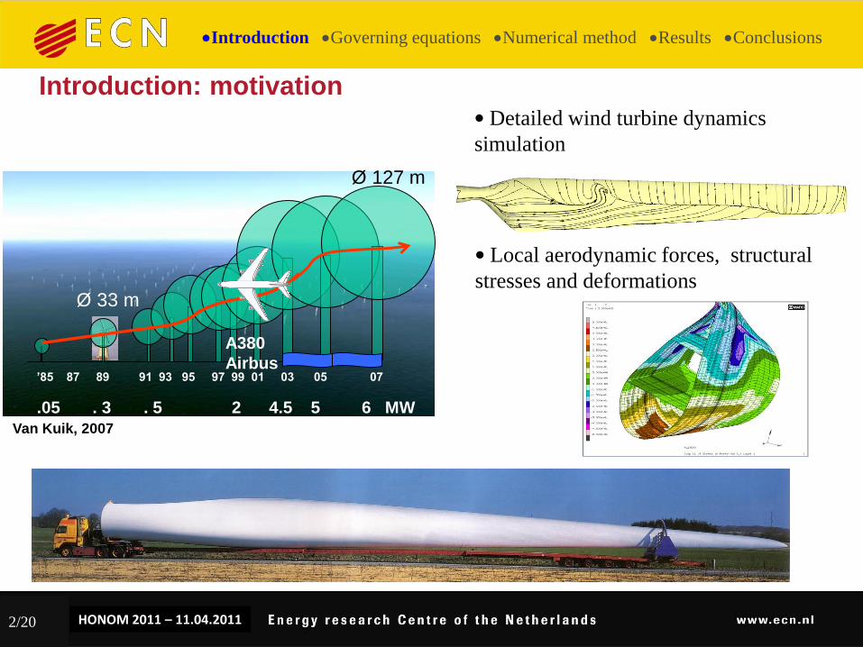
Introduction: motivation • Detailed wind turbine dynamics

simulation

• Local aerodynamic forces, structural

stresses and deformations

Introduction Governing equations Numerical method Results Conclusions

Ø 127 m

’85 87 89 91 93 95 97 99 01 03 05 07

.05 . 3 . 5 2 4.5 5 6 MW

Ø 33 m

A380

Airbus

Van Kuik, 2007

EFMC8 - 16.09.2010 HONOM 2011 – 11.04.2011 3/20

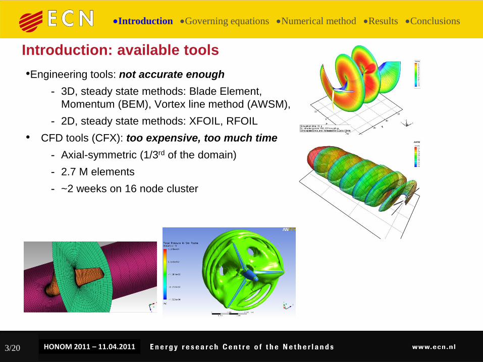
•Engineering tools: not accurate enough

- 3D, steady state methods: Blade Element,

Momentum (BEM), Vortex line method (AWSM),

- 2D, steady state methods: XFOIL, RFOIL

• CFD tools (CFX): too expensive, too much time

- Axial-symmetric (1/3rd of the domain)

- 2.7 M elements

- ~2 weeks on 16 node cluster

Introduction: available tools

Introduction Governing equations Numerical method Results Conclusions

EFMC8 - 16.09.2010 HONOM 2011 – 11.04.2011 4/20

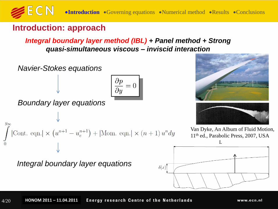
Van Dyke, An Album of Fluid Motion,

11th ed., Parabolic Press, 2007, USA

Introduction: approach

Introduction Governing equations Numerical method Results Conclusions

Integral boundary layer method (IBL) + Panel method + Strong

quasi-simultaneous viscous – inviscid interaction

Navier-Stokes equations

Boundary layer equations

Integral boundary layer equations

EFMC8 - 16.09.2010 HONOM 2011 – 11.04.2011 5/20

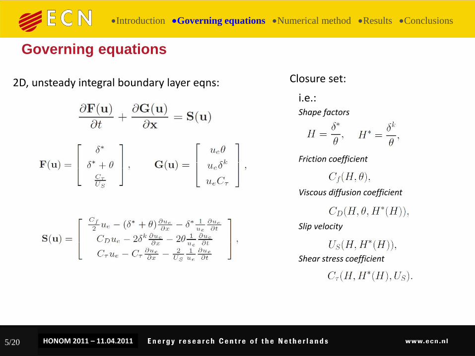
Governing equations

Introduction Governing equations Numerical method Results Conclusions

2D, unsteady integral boundary layer eqns: Closure set:

Shape factors

Friction coefficient

Viscous diffusion coefficient

Slip velocity

Shear stress coefficient

i.e.:

EFMC8 - 16.09.2010 HONOM 2011 – 11.04.2011 6/20

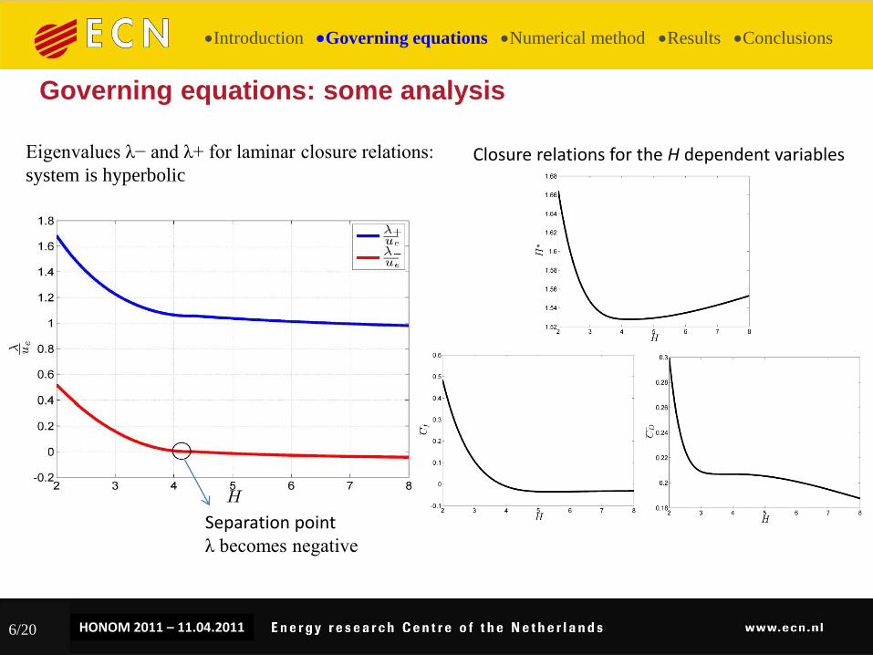
Governing equations: some analysis

Eigenvalues λ− and λ+ for laminar closure relations:

system is hyperbolic

Introduction Governing equations Numerical method Results Conclusions

Separation point λ becomes negative

Closure relations for the H dependent variables

EFMC8 - 16.09.2010 HONOM 2011 – 11.04.2011 7/20

Introduction Governing equations Numerical method Results Conclusions

Numerical method: Discontinuous Galerkin (DG) Method

Weak formulation

Solution vector:

Approximate solution

Discrete equation

EFMC8 - 16.09.2010 HONOM 2011 – 11.04.2011 8/20

Introduction Governing equations Numerical method Results Conclusions

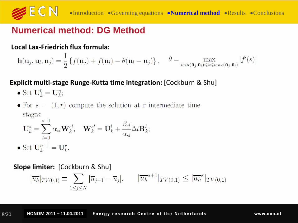
Numerical method: DG Method

Local Lax-Friedrich flux formula:

Explicit multi-stage Runge-Kutta time integration: [Cockburn & Shu]

Slope limiter: [Cockburn & Shu]

EFMC8 - 16.09.2010 HONOM 2011 – 11.04.2011 9/20

Introduction Governing equations Numerical method Results Conclusions

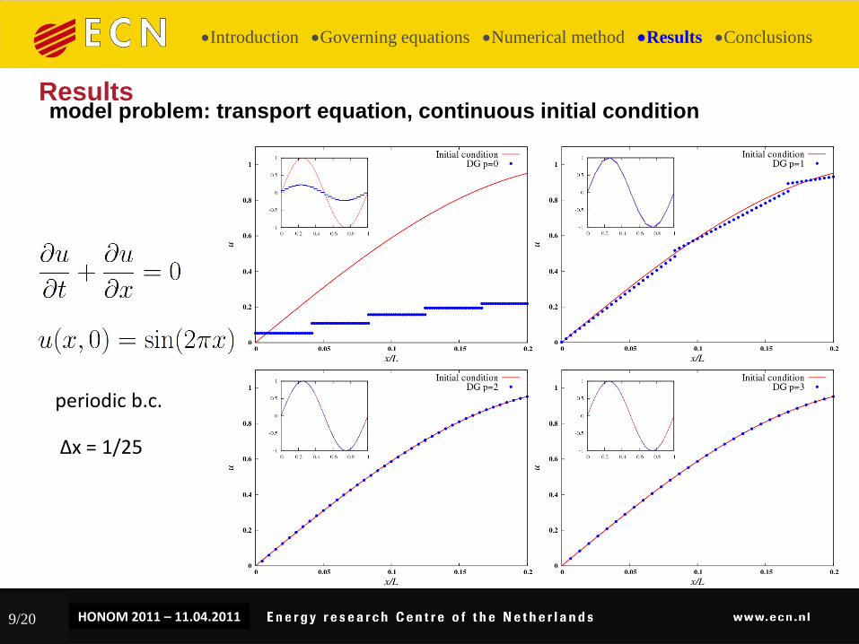
Results model problem: transport equation, continuous initial condition

periodic b.c.

Δx = 1/25

EFMC8 - 16.09.2010 HONOM 2011 – 11.04.2011 10/20

Introduction Governing equations Numerical method Results Conclusions

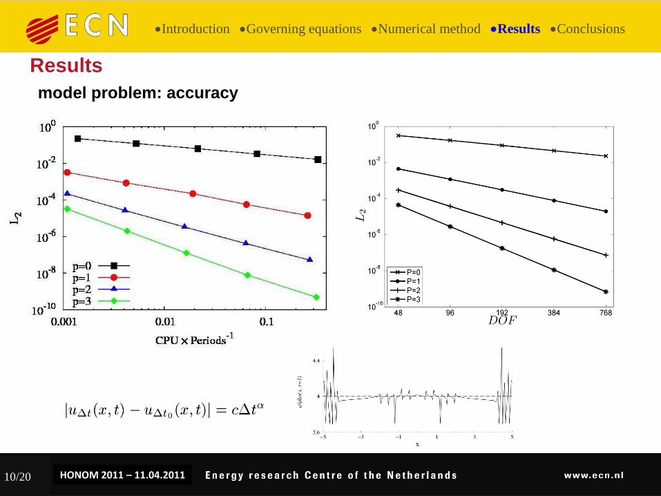
Results

model problem: accuracy

EFMC8 - 16.09.2010 HONOM 2011 – 11.04.2011

Introduction Governing equations Numerical method Results Conclusions

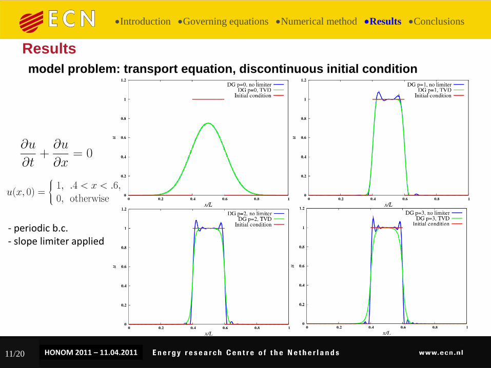
Results

model problem: transport equation, discontinuous initial condition

- periodic b.c. - slope limiter applied

11/20

EFMC8 - 16.09.2010 HONOM 2011 – 11.04.2011

Introduction Governing equations Numerical method Results Conclusions

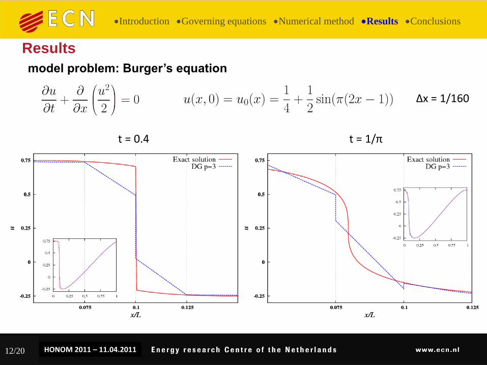
Results

model problem: Burger’s equation

12/20

t = 0.4 t = 1/π

Δx = 1/160

EFMC8 - 16.09.2010 HONOM 2011 – 11.04.2011 13/20

Introduction Governing equations Numerical method Results Conclusions

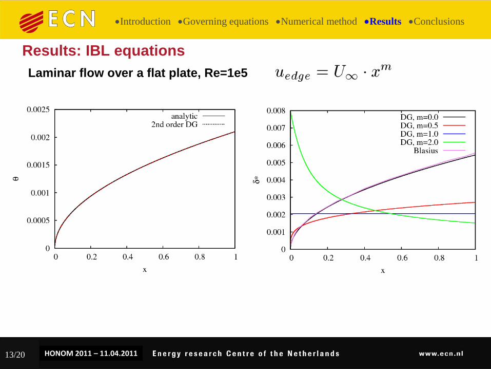
Results: IBL equations

Laminar flow over a flat plate, Re=1e5

EFMC8 - 16.09.2010 HONOM 2011 – 11.04.2011 14/20

Introduction Governing equations Numerical method Results Conclusions

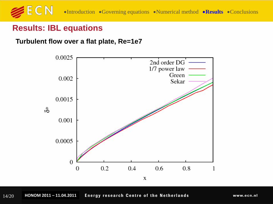
Turbulent flow over a flat plate, Re=1e7

Results: IBL equations

EFMC8 - 16.09.2010 HONOM 2011 – 11.04.2011 15/20

Introduction Governing equations Numerical method Results Conclusions

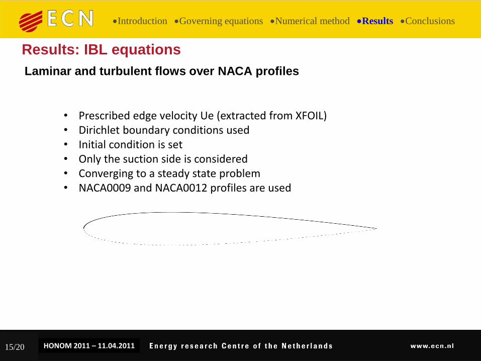
Results: IBL equations

Laminar and turbulent flows over NACA profiles

• Prescribed edge velocity Ue (extracted from XFOIL) • Dirichlet boundary conditions used • Initial condition is set • Only the suction side is considered • Converging to a steady state problem • NACA0009 and NACA0012 profiles are used

EFMC8 - 16.09.2010 HONOM 2011 – 11.04.2011 16/20

Introduction Governing equations Numerical method Results Conclusions

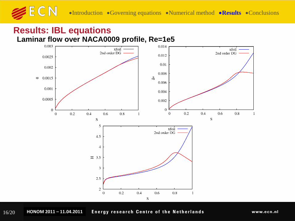
Results: IBL equations Laminar flow over NACA0009 profile, Re=1e5

EFMC8 - 16.09.2010 HONOM 2011 – 11.04.2011 17/20

Introduction Governing equations Numerical method Results Conclusions

Results: IBL equations Turbulent flow over NACA0012 profile, Re=1e5

EFMC8 - 16.09.2010 HONOM 2011 – 11.04.2011 18/20

Introduction Governing equations Numerical method Results Conclusions

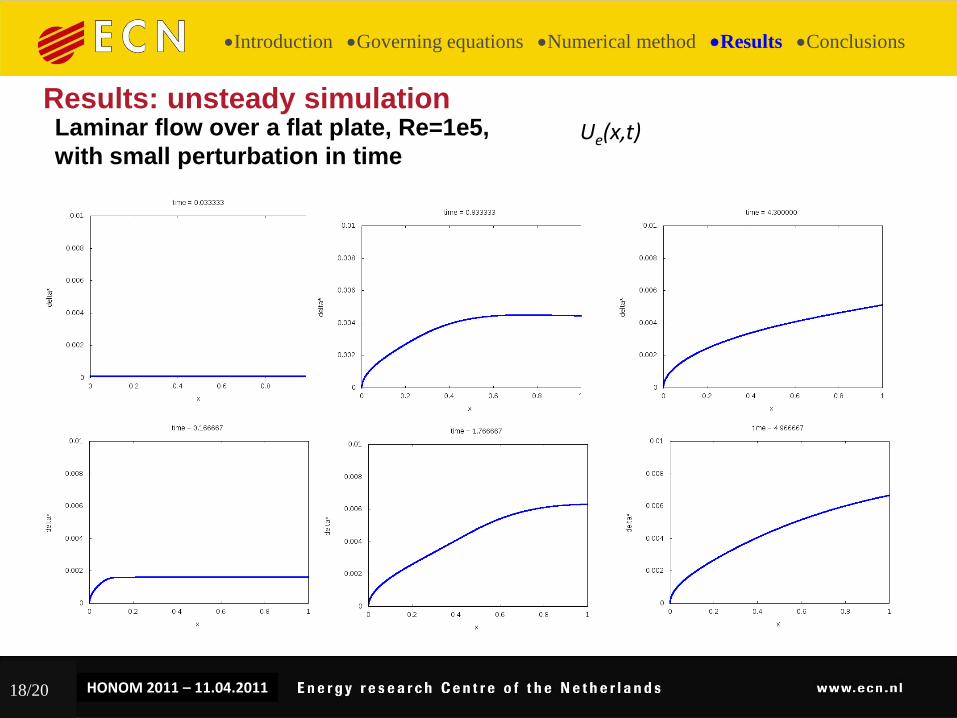
Results: unsteady simulation Laminar flow over a flat plate, Re=1e5,

with small perturbation in time Ue(x,t)

EFMC8 - 16.09.2010 HONOM 2011 – 11.04.2011 19/20

Introduction Governing equations Numerical method Results Conclusions

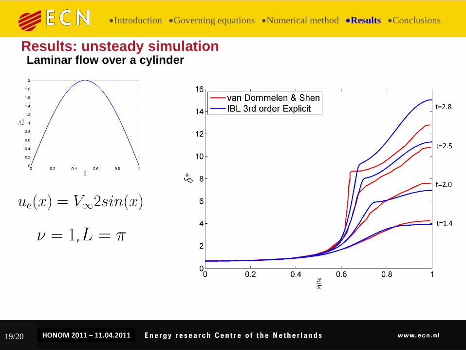
Results: unsteady simulation Laminar flow over a cylinder

,

EFMC8 - 16.09.2010 HONOM 2011 – 11.04.2011 20/20

Fully laminar and turbulent flows over a flat plate

show good agreement with the literature

Flow over NACA profiles are in good agreement

up to separation point

Non-conservative implementation

TVBM slope limiter will be implemented

More experimental data needed for 3D unsteady

boundary layers and also for rotational effects

Introduction Governing equations Numerical method Results Conclusions

Conclusions and Outlook

EFMC8 - 16.09.2010 HONOM 2011 – 11.04.2011

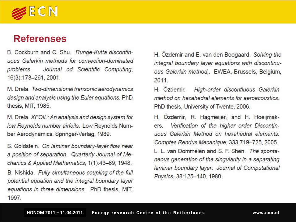
Referenses