Artificial Boundary Conditions for the

Numerical Simulation of Unsteady Acoustic

Waves

S. V. Tsynkov 1

Department of Mathematics and Center for Research in Scientific Computation(CRSC), North Carolina State University, Box 8205, Raleigh, NC 27695, USA.

Abstract

We construct non-local artificial boundary conditions (ABCs) for the numerical sim-ulation of genuinely time-dependent acoustic waves that propagate from a compactsource in an unbounded unobstructed space. The key property used for obtainingthe ABCs is the presence of lacunae, i.e., sharp aft fronts of the waves, in wave-typesolutions in odd-dimension spaces. This property can be considered a manifestationof the Huygens’ principle. The ABCs are obtained directly for the discrete formula-tion of the problem. They truncate the original unbounded domain and guaranteethe complete transparency of the new outer boundary for all the outgoing waves. Acentral feature of the proposed ABCs is that the extent of their temporal nonlocalityis fixed and limited, and it does not come at the expense of simplifying the originalmodel. It is rather a natural consequence of the existence of lacunae, which is a fun-damental property of the corresponding solutions. The proposed ABCs can be builtfor any consistent and stable finite-difference scheme. Their accuracy can alwaysbe made as high as that of the interior approximation, and it will not deteriorateeven when integrating over long time intervals. Besides, the ABCs are most flexiblefrom the standpoint of geometry and can handle irregular boundaries on regulargrids with no fitting/adaptation needed and no accuracy loss induced. Finally, theyallow for a wide range of model settings. In particular, not only one can analyze thesimplest advective acoustics case with the uniform background flow, but also thecase when the waves’ source (or scatterer) is engaged in an accelerated motion.

Key words: Time-dependent sound waves, unbounded domains, lacunae,non-deteriorating method, long-term computation, limited temporal nonlocality.

Email address: tsynkov@math.ncsu.edu (S. V. Tsynkov).URL: http://www.math.ncsu.edu/∼stsynkov (S. V. Tsynkov).

1 The author gratefully acknowledges support by AFOSR, Grant F49620-01-1-0187,and that by NSF, Grant DMS-0107146.

1 Introduction

Artificial Boundary Conditions (ABCs) is a common name for a group ofmethods employed for solving infinite-domain problems on a computer. ABCsfacilitate truncation of the original unbounded domain, and provide the re-quired closure for the resulting truncated formulation. The literature on thesubject of ABCs is broad, and we refer the reader to the review papers [1–3].

Two opposite trends can be identified in building the ABCs. High accuracyrequirements typically imply that the ABCs should be nonlocal. In partic-ular, the exact ABCs are always nonlocal in multidimensional settings. Forunsteady problems, this also means nonlocality in time. Clearly, nonlocalityof the ABCs may result in high computational costs and elaborate implemen-tation strategies. As such, local alternatives obtained either independently oras a approximations of nonlocal ABCs become viable. These ABCs are usuallyinexpensive and easy to implement, but may lack computational accuracy.

In the current paper we propose the ABCs for the numerical simulation ofnon-dispersive unsteady acoustic waves. We assume that there is a (complex)phenomenon/process confined to a bounded region that manifests itself by theradiation of acoustic waves in the far field. The waves subsequently propagateacross the unbounded and unobstructed space, which is assumed isotropicand homogeneous. The proposed ABCs are nonlocal and guarantee that theaccuracy of the boundary treatment can always be made at least as high asthat of the interior discretization. However, the key feature of the proposedABCs is that the extent of their temporal nonlocality is limited, and does notincrease as the time elapses. The bound on temporal nonlocality comes as aconsequence of the presence of lacunae, i.e., sharp aft fronts of the waves, inthe solutions of the linearized Euler equations. In general, existence of thelacunae is a fundamental property of wave-type solutions in odd-dimensionspaces. It is often referred to in connection with the Huygens’ principle.

The ABCs are constructed by decomposing the original problem into the inte-rior and auxiliary sub-problems. The latter is linear and homogeneous through-out the entire space, and is integrated with the help of lacunae. In so doing,the interior solution is used to generate sources for the auxiliary problem, andthe auxiliary solution is used to provide the missing boundary data, i.e., therequire closure, for the interior problem.

Several other nonlocal ABCs’ methodologies for unsteady waves have beenrecently advocated in the literature, most notably [4–10]; we also mention thesurvey paper [11] and the bibliography there. Compared to these techniques,our approach has a number of distinctive characteristics. Its high accuracy andrestricted temporal nonlocality have already been mentioned. Besides, the pro-

2

posed lacunae-based ABCs are obtained directly for the discrete formulationof the problem, and can supplement any consistent and stable finite-differencescheme. In other words, they bypass the common stages of first deriving andthen approximating the continuous ABCs, see [2]. The lacunae-based ABCsare especially designed to withstand long-term numerical integration with nodeterioration of accuracy. Moreover, neither they are restricted to any par-ticular shape of artificial boundary nor require grid fitting. They also enableanalysis of a variety of problem formulations, e.g., the case of sound sourcesmoving with acceleration, which is equivalent to advective acoustics with un-steady background flow. We note that the source motion does not have to beconsidered relative to an ambient medium only. Via the appropriate Galileotransform, it can be considered relative to a given mean flow as well.

The ABCs that we derive in the current paper for acoustics generalize andfurther extend our previous work [12,13], in which a similar methodology wasintroduced for the scalar wave equation. The current approach also fits intothe general theoretical framework of [14].

2 Lacunae of the Wave Equation

Consider a three-dimensional wave equation, x = (x1, x2, x3):

1

c2

∂2ϕ

∂t2−(∂2ϕ

∂x21

+∂2ϕ

∂x22

+∂2ϕ

∂x23

)= f(x , t), t ≥ 0, (1a)

ϕ∣∣∣∣t=0

=∂ϕ

∂t

∣∣∣∣∣t=0

= 0, (1b)

with homogeneous initial conditions. For every (x , t), the solution ϕ = ϕ(x , t)of problem (1a), (1b) is given by the Kirchhoff integral (see, e.g., [15]):

ϕ(x , t) =1

4π

∫∫∫%≤ct

f (ξ, t− %/c)%

dξ, (2)

where ξ = (ξ1, ξ2, ξ3), % = |x − ξ| =√

(x1 − ξ1)2 + (x2 − ξ2)2 + (x3 − ξ3)2,

and dξ = dξ1dξ2dξ3. If we assume that the right-hand side (RHS) f(x , t)of equation (1a) is compactly supported in space-time on the domain Q ⊂R

3 × [0,+∞), then formula (2) immediately implies that

ϕ(x , t) ≡ 0 for (x , t) ∈⋂

(ξ,τ)∈Q

{(x , t)

∣∣∣|x − ξ| < c(t− τ), t > τ}. (3)

The region of space-time defined by formula (3) is called lacuna of the solutionϕ = ϕ(x , t). This region is obtained as the intersection of all characteristic

3

cones of equation (1a) once the vertex of the cone sweeps the support of theRHS: supp f ⊆ Q. From the standpoint of physics, lacuna corresponds tothat part of space-time, on which the waves generated by the sources f(x , t),supp f ⊆ Q, have already passed, and the solution has become zero again.The phenomenon of lacunae is inherently three-dimensional. The surface ofthe lacuna represents the trajectory of aft (trailing) fronts of the waves. Theexistence of aft fronts in odd-dimension spaces is known as the Huygens’ prin-ciple, as opposed to the so-called wave diffusion which takes place in even-dimension spaces, see, e.g., [15]. Let us also note that the aft fronts and thelacunae would still be present in the solution of the wave equation (1a) if thehomogeneous initial conditions (1b) were replaced by some inhomogeneousinitial conditions with compact support.

The notion of lacunae (or lacunas) was first introduced and studied byPetrowsky in [16] (see also an account in [17, Chapter VI]) for a variety ofhyperbolic equations and systems; and general characterization of their coef-ficients was provided that would guarantee existence of the lacunae. However,since work [16] no constructive examples of either equations or systems havebeen obtained for which lacunae would be present in the solutions, besides theactual wave equation (1a), as well as those equations that either reduce to orare derived from, the wave equation.

3 The Acoustics System of Equations

The acoustics (linearized Euler’s) system in its simplest form governs thepropagation of sound in an ambient compressible fluid [18, Chapter VIII]:

1

c2

∂p

∂t+ ρ0∇ · u = ρ0qvol,

ρ0∂u

∂t+∇p = bvol.

(4)

In (4), c is the speed of sound, and the variables u = u(x , t) and p = p(x , t)represent small perturbations of the velocity and pressure, respectively. Adi-abatic law p = c2ρ has been applied that relates p to the density perturba-tion ρ. The quantity ρ0 is the constant background density. The source termqvol = qvol(x , t) that alters the balance of mass in the system is known as vol-ume velocity per unit volume, and the source term bvol = bvol(x , t) that altersthe balance of momentum is known as force per unit volume (see, e.g., [19]).

Proposition 1 Assume that the initial velocity field is conservative:u(x , 0) = ∇ϕ0(x ). Then, the velocity potential exists in the solutions ofsystem (4) for all t ≥ 0 if and only if the forcing bvol is also conservative:bvol(x , t) = ∇ψ(x , t). In this case, the potential satisfies the wave equation.

4

PROOF. Let us assume that the force field is conservative, and integrate thesecond equation of system (4) with respect to time starting from t = 0:

ρ0u(x , t) = ρ0u(x , 0)−∫ t

0∇p(x , τ)dτ +

∫ t

0bvol(x , τ)dτ

= ρ0∇ϕ0(x )−∫ t

0∇p(x , τ)dτ +

∫ t

0∇ψ(x , τ)dτ

= ∇[ρ0ϕ0(x )−

∫ t

0p(x , τ)dτ +

∫ t

0ψ(x , τ)dτ

]def= ρ0∇ϕ(x , t).

(5)

Therefore, we obtain:

u(x , t) = ∇ϕ(x , t), ρ0∂ϕ(x , t)

∂t= −p(x , t) + ψ(x , t), (6)

and by differentiating the second relation in (6) w.r.t. time and subsequentlysubstituting it into the first equation of system (4), we conclude that thepotential ϕ = ϕ(x , t) defined by (5) will satisfy the wave equation (1a) with

the RHS given by f(x , t) = −qvol(x , t) + 1ρ0c2

∂ψ(x ,t)∂t

.

Conversely, let us assume that the velocity field is conservative: u(x , t) =∇ϕ(x , t). Then, the momentum equation in system (4) can be recast as follows:

∇[ρ0∂ϕ

∂t+ p

]= bvol,

which means that the forcing must be conservative: bvol(x , t) = ∇ψ(x , t). 2

Proposition 1 also implies that if bvol(x , t) ≡ 0 then the potential always exists.In this case, the second equality of (6) reduces to the conventional relationbetween the potential and pressure: ρ0

∂ϕ∂t

= −p, see [18, Chapter VIII].

Applying the gradient operator to the wave equation for the potential, weconclude that the velocity vector also satisfies the wave equation:

1

c2

∂2u

∂t2−∆u = −∇qvol +

1

ρ0c2

∂bvol

∂t. (7)

Next, by differentiating the first equation of (4) with respect to time, takingthe divergence of the second equation of (4), and substituting the result intothe first one, we arrive at the wave equation for p:

1

c2

∂2p

∂t2−∆p = −∇ · bvol + ρ0

∂qvol

∂t. (8)

5

The key consideration of interest is that if the RHSs of system (4) are com-pactly supported in space and time on some domain Q ⊂ R3 × [0,+∞), thenthe RHSs of both equation (7) and equation (8) will also be compactly sup-ported on the same domain Q. Consequently, solutions of equations (7) and(8) will have lacunae of the same shape as prescribed by formula (3). Thus,we have arrived at the following

Proposition 2 Let the RHSs of system (4) be compactly supported in spaceand time: supp qvol(x , t) ⊆ Q and supp bvol(x , t) ⊆ Q, where Q ⊂ R

3 ×[0,+∞). Let also u(x , t) = ∇ϕ(x , t). Then, solutions of the acoustics sys-tem (4) with homogeneous initial conditions will have lacunae of the samegeometry as provided by formula (3).

In other words, we have shown that existence of the velocity potential is suf-ficient for the acoustics system (4) to have lacunae in its solutions; and thatthe geometry of the lacunae is determined by that of the support of the RHSs,as in the case of the wave equation. We do not know whether this conditionis also necessary for having the lacunae. However, in the view of the commentprovided in the end of Section 2, we will hereafter be using the foregoing suf-ficient condition as the only reliable indication of the presence of lacunae inthe solutions of system (4).

The group of numerical algorithms for acoustics that we describe hereafterwill be essentially based on the presence of lacunae. However, the Kirchhoffformula (2) will never be used as an actual part of the algorithm construction,it will only be needed at the theoretical stage, for determining the shape ofthe lacunae that will later be incorporated into a purely finite-difference con-text. Previously, the idea of using the Huygens’ principle for constructing theABCs was promoted by Ting & Miksis [20] and Givoli & Cohen [21]. Bothpapers, however, have suggested to use numerical quadratures to approximatethe integral (2), and then couple it with the interior solution. Moreover, theapproach of [20] has never been actually implemented in a practical compu-tational setting, whereas the approach of [21] required artificial dissipation tobe added to the scheme to fix the arising instabilities.

4 Lacunae-Based Integration of the Acoustics System

We will be looking for an irrotational solution of system (4) on a boundeddomain S = S(t) ⊂ R

3. We assume that this is a domain of fixed shapethat has a finite diameter d for all t ≥ 0. We also assume that ∀t ≥ 0 :{supp qvol(x , t) ∩ R3} ⊆ S(t) & {supp bvol(x , t) ∩ R3} ⊆ S(t). In other words,we want to compute the acoustic field on a given domain that also containsall the field sources. While always remaining finite in size, this domain S(t) is

6

allowed to move across the space R3 according to a general law:

u0 = u0(t), x0 = x0(t) =∫ t

0u0(τ)dτ, (9)

where u0 and x0 are the velocity vector and coordinates of a given point in-side S(t), respectively. The only limitation that we impose is that motion (9)be subsonic: maxt |u0(t)| = k < c. Let now qvol and bvol be some station-ary acoustic sources (RHSs to system (4)), i.e., compactly supported func-tions of x on the fixed domain S(0) for all t ≥ 0: {supp qvol(x , t) ∩ R3} ⊆S(0) & {supp bvol(x , t) ∩ R3} ⊆ S(0). Then, we can incorporate the transla-tional motion (9) into the acoustics system (4) as follows, see [12]:

1

c2

∂p(x , t)

∂t+ ρ0∇ · u(x , t) = ρ0qvol(x − x0(t), t) ≡ ρ0qvol(x , t),

ρ0∂u(x , t)

∂t+∇p(x , t) = bvol(x − x0(t), t) ≡ bvol(x , t).

(10)

With no loss of generality, the initial conditions for integrating system (10)will always be assumed homogeneous. It is easy to see from (10) that the time-dependent nature of the acoustic field is caused by the motion of the soundsources, on which the genuine unsteadiness of the sound generating mecha-nisms may be “superimposed.” The domain of integration S(t) has a fixedsize/shape and traces the motion of the sources. As shown in [12, Appendix]using the Galileo transform, system (10) is equivalent to advective acousticswith stationary sources and unsteady background flow −u0 = −u0(t).

Let us emphasize that the setup we have introduced is quite general and alsoincludes the case of the waves’ sources that move relative to a given mean flow(rather than relative to the ambient fluid only). Indeed, a similar argumentbased on the Galileo transform would imply that having the mean flow v0 andthe source motion u0 on top of it is equivalent to either stationary sources inthe mean flow v0 − u0 or alternatively, sources that move with the velocity−v0 +u0 through the ambient medium. The latter setup is obviously the sameas (9), as long as the condition maxt | − v0(t) + u0(t)| = k < c is met.

The case of primary interest for our analysis will be that of continuouslyoperating sources in (10), t ∈ [0,+∞). Let us, however, assume for the timebeing that not only the RHSs in system (10) are compactly supported inspace, but also that their “lifespan” in time is finite: supp qvol(x , t) ∈ Q and

supp bvol(x , t) ∈ Q, where R3 × [0,+∞) 3 Q = {(x , t)∣∣∣x ∈ S(t), t0 ≤ t ≤ t1}.

Then, Proposition 2 implies that no later than

t = t2 ≡ t0 +d+ (t1 − t0)(c+ k)

c− k≡ t0 + Tint (11)

all of the domain S(t) will fall into the lacuna defined by formula (3) (see

7

[12,13] for a more detailed argument), and will remain inside the lacuna con-tinuously thereafter, i.e., for all t ≥ t2. In other words, for the solution ofsystem (10), we will have p(x , t) = 0 and u(x , t) = 0 when x ∈ S(t) andt ≥ t2, where t2 is defined by formula (11).

Next, we realize that during the time interval Tint no wave can travel inspace further away than the distance cTint from the boundary of the domainS(t0). This means that we will also have p(x , t) = 0 and u(x , t) = 0 fordist (x , S(t0)) > cTint and t0 ≤ t ≤ t2. As such, instead of the free unob-structed space outside S(t) we may consider outer boundaries with arbitrary(reflecting) properties. As long as none of these boundaries is located closerthan cTint to S(t0), the solution of (10) inside S(t) is not going to feel theirpresence for t0 ≤ t ≤ t2.

In fact, the foregoing limitation for the location of outer boundaries can evenbe relaxed if instead of requiring that no wave may reach an outer boundarybefore t = t2 we introduce a weaker requirement that no reflected wave mayreach S(t) before t = t2. The latter consideration easily translates into thefollowing estimate for the minimal distance between the domain S(t0) and theallowed location of any reflecting boundary (see [12,13] for more detail):

Zmin =c+ k

2Tint. (12)

We note that both estimates (11) and (12) are conservative in the sense thatthey do not take into account the direction of the motion. In case the motionof the sources is characterized by a specific or predominant direction, then thequantity Zmin can be further reduced in the orthogonal directions.

Altogether we conclude that the solution of system (10) driven by the sources

compactly supported on the domain Q = {(x , t)∣∣∣x ∈ S(t), t0 ≤ t ≤ t1} and

subject to the homogeneous initial conditions, can be obtained on S(t) for allt ≥ 0 as follows. First, this solution is obviously equal to zero for 0 ≤ t < t0.Next, on the time interval t0 ≤ t ≤ t2, see formula (11), system (10) shouldbe integrated on the auxiliary domain of size

Z = d+ 2Zmin = d+ (c+ k)Tint (13)

centered around S(t0), which in any event is going to yield the correct solutioninside S(t). Finally, for all t ≥ t2 the solution on S(t) will be equal to zeroagain because all the waves will have left the domain by t = t2 (lacuna).

Let us now address the case of continuously operating sources. For that pur-

8

pose, we introduce a partition of unity on the semi-infinite interval t ≥ 0:

∀t ≥ 0 :∞∑j=0

Θ(t− σTj) = 1, (14)

where T > 0 and 12≤ σ < 1 are two parameters, and Θ = Θ(t) is a smooth,

even, “hat”-type function with supp Θ(t) ⊆ [−T2, T

2]:

Θ(t) =

0, t > T

2,

1, 0 ≤ t ≤ (σ − 12)T,

1−Θ(σT − t), (σ − 12)T < t ≤ T

2,

Θ(−t), t < 0.

(15)

Then, we define compactly supported sources for j = 0, 1, 2, . . . :

q(j)vol(x , t) = qvol(x , t)Θ(t− σTj), supp q

(j)vol(x , t) ⊆ Qj,

b(j)vol(x , t) = bvol(x , t)Θ(t− σTj), supp b

(j)vol(x , t) ⊆ Qj,

(16)

where according to (15):

Qj ={

(x , t)∣∣∣x ∈ S(t),

(σj − 1

2

)T ≤ t ≤

(σj +

1

2

)T}, (17)

and consider a collection of sub-problems driven by the RHSs (16):

1

c2

∂p(j)

∂t+ ρ0∇ · u (j) = ρ0q

(j)vol,

p(j)(x , t)∣∣∣t=(σj− 1

2)T

= 0,

ρ0∂u (j)

∂t+∇p(j) = b

(j)vol ,

u (j)(x , t)∣∣∣t=(σj− 1

2)T

= 0.

(18)

As formula (14) is a partition of unity, we have:

qvol(x , t) =∞∑j=0

q(j)vol(x , t) and bvol(x , t) =

∞∑j=0

b(j)vol(x , t),

and because of the linear superposition, the solution p(x , t), u(x , t) of system(10) subject to the homogeneous initial conditions at t = 0 can be expandedin terms of the solutions to systems (18):

p(x , t) =∞∑j=0

p(j)(x , t) and u(x , t) =∞∑j=0

u (j)(x , t). (19)

The series (19) are formally infinite. However, for any t > 0 and x ∈ S(t) eachwill, in fact, contain only a finite fixed number of nonzero terms. Indeed, dueto the causality for a given t > 0 and all (σj− 1

2)T > t, i.e., all j > ( t

T+ 1

2)/σ,

we will have p(j)(x , t) = 0 and u (j)(x , t) = 0 on the entire space R3. Moreover,

9

multiplication by the function Θ, see (16), that is only a function of time willnot alter the conservative nature of bvol. Therefore, Proposition 2 will applyto the solution of every problem (18), j = 0, 1, 2, . . . . As such, if we interpret

the moment (σj − 12)T of the inception of source j as t

(j)0 , and the moment

(σj + 12)T of its cessation as t

(j)1 , then according to formula (11):

∀t >(σj − 1

2

)T +

d+ T (c+ k)

c− k≡ t

(j)0 + Tint :

p(j)(x , t) = 0 and u (j)(x , t) = 0 for x ∈ S(t),

(20)

i.e., the domain S(t) will be entirely inside the lacuna starting from t(j)2 =

t(j)0 +Tint. Alternatively, this means that for any t > 0 and all j < ( t−Tint

T+ 1

2)/σ,

where Tint = d+T (c+k)c−k as in formula (20), the terms p(j)(x , t) and u (j)(x , t) in

the series (19) will be equal to zero for x ∈ S(t). Consequently, for all t > 0and x ∈ S(t) we can replace expansions (19) with

p(x , t) =m2∑j=m1

p(j)(x , t) and u(x , t) =m2∑j=m1

u (j)(x , t), (21)

where m1 =[( t−Tint

T+ 1

2)/σ

], m2 =

[( tT

+ 12)/σ

]+ 1, and [ · ] denotes the

integer part. This implies that for any t > 0 and x ∈ S(t) the number ofterms m = m2−m1 + 1 in the sum (21), and as such, the number of non-zero

terms in the expansion (19), may not exceed[Tint

σT

]+ 2. Most important, this

number m does not increase as the time t elapses, because the interval Tint

introduced in (20) depends only on the partition size T for the sources, thegeometry, the propagation speed, and the maximum speed of motion.

Let us now assume that each problem (18) is integrated individually on anappropriate domain of size Z, see formula (13), by means of a consistent andstable finite-difference scheme. For every given j, system (18) only needs to be

integrated from t(j)0 = (σj− 1

2)T till t

(j)2 = t

(j)0 +Tint because for all subsequent

moments of time its solution on S(t) will be equal to zero. Consequently, the

following convergence estimates will hold for t(j)0 ≤ t ≤ t

(j)2 and x ∈ S(t):

‖p(j)(x , t)− p(j)h (x , t)‖ ≤ Kjh

α,

‖u (j)(x , t)− u(j)h (x , t)‖ ≤ Kjh

α,(22)

where α is the order of convergence, h denotes the generic grid size, and thefunctions p

(j)h (x , t) and u

(j)h (x , t) denote the discrete solution of system (18)

for a given j. The constant Kj on the right-hand side of each inequality (22)

does not depend on h, but may depend on q(j)vol and b

(j)vol , as well as on Tint.

We emphasize that the quantity Tint does not depend on j. Moreover, it is nat-ural to assume that the derivatives of the functions q

(j)vol(x , t) and b

(j)vol(x , t) are

10

uniformly bounded with respect to j. In this case, there will be a j-independentconstant K = K(qvol, bvol, Tint) such that ∀j = 0, 1, 2, . . . : Kj ≤ K. Then,using representations (21) one can easily transform the individual convergenceestimates (22) into the overall temporally uniform grid convergence estimatefor p and u that would hold for t ≥ 0 and x ∈ S(t):

‖p(x , t)− ph(x , t)‖ ≤ mKhα,

‖u(x , t)− uh(x , t)‖ ≤ mKhα.(23)

In formulae (23), ph(x , t) =m2∑j=m1

p(j)h (x , t) and uh(x , t) =

m2∑j=m1

u(j)h (x , t). A

detailed proof of this result for the wave equation can be found in [12].

In practical terms, the temporally uniform grid convergence guaranteed byestimates (23) means that accuracy of the numerical solution of system (10),if computed using lacunae, i.e., by solving a set of systems (18) and then em-ploying representation (21), will not deteriorate even when system (10) is inte-grated over arbitrarily long time intervals. In other words, one should expectthat there will be no long-time error buildup. This is, in fact, a key distinctionbetween the foregoing lacunae-based algorithm and traditional time-marchingtechniques that may be applied to computing the unsteady acoustic fields.

Indeed, the phenomenon of error accumulation during long runs is well-knownin the context of building computational methods for time-dependent prob-lems. This issue has been recognized in the literature as an outstanding unre-solved question in numerical PDEs for many years, since the first systematicconvergence studies for discrete approximations have been conducted in thefifties. At the analysis stage, it manifests itself by the growth of the stabilityconstants with time. If, for example, system (10) needs to be integrated overthe interval [0, Tfinal], then the stability constant of the scheme will, generallyspeaking, depend on Tfinal: K = K( · , Tfinal), and will actually increase withthe increase of Tfinal. This is, of course, the exact same phenomenon as the de-pendence of Kj on Tint in formulae (22). The growth of the stability constantswith Tfinal is equivalent to non-uniformity of the grid convergence in time, andall conventional discrete approximations that can be and are used in modernnumerical methods are known to suffer from this deficiency. In practice, thisimplies that any given approximation can be used for only a limited intervalof time if the acceptable level of error is prescribed. To advance further intime with no loss of accuracy a finer approximation is needed from the verybeginning, which obviously prompts the increase of the overall computationalcost. The latter increase may quickly become prohibitive.

Using the language of wave physics, one can, e.g., attribute the long-term errorbuildup to either numerical dissipation, or dispersion (phase error), or both.But no matter what its actual mechanism is, it may result in an unacceptable

11

loss of accuracy by the solution within a finite period of time.

The lacunae-based algorithm allows us to circumvent this difficulty due to thetemporally uniform convergence (23). Moreover, if system (10) were to be in-tegrated on the large interval [0, Tfinal] using a straightforward time-marchingalgorithm, it would have also required a large domain in space, of the sizeroughly 2cTfinal. This is typically not feasible. On the other hand, implemen-tation of the lacunae-based algorithm allows us to perform the integration onthe domain of a fixed and non-increasing size Z determined by formula (13).

It is important to mention that smoothness plays a key role in the design of thelacunae-based algorithm. In particular, the function Θ(t) of (15) that helps usbuild the partition of unity (14) has to be chosen sufficiently smooth so thatthe dependence of the stability constants Kj on the properties of individual

RHSs q(j)vol and b

(j)vol , see (22), be not worse than that in the original scheme with

non-partitioned source terms. In this paper, we leave out the detailed analysisthat involves the quantitative smoothness characteristics, and instead referthe reader to our previous work [12].

Implementation of the lacunae-based algorithm now needs to be discussed. Intheory, system (18) for every given j = 0, 1, 2, . . . should be integrated on its

own auxiliary region of size Z, see (13), centered around the domain S(t(j)0 ),

where t(j)0 = (σj − 1

2)T and the location of S(t

(j)0 ) is, in turn, determined by

the reference point x0(t(j)0 ), see formula (9). However, it is more convenient

to consider periodic boundary conditions with the period Z in all coordinatedirections. In this case, motion (9) should be interpreted as the motion on athree-dimensional toroidal surface, and all spatial locations shall be convertedto the periodic setting: x 7→ x ≡ (x1, x2, x3), where xi = xi − [xi

Z]Z, i =

1, 2, 3. In so doing, all systems (18) can basically be solved on one and thesame domain with periodic boundary conditions, because it obviously doesnot matter where on the period the “initial” domain S(t

(j)0 ) is located for

every j = 0, 1, 2, . . . . Moreover, while the most universal formulation wouldimply choosing the same period Z for all the coordinates, in the case whenmotion (9) is characterized by a predominant direction, the periods in thedirections orthogonal to that can be chosen smaller. For subsequent analysisin the current paper, the periodic setup will always be assumed.

Next, let us recast each formula (21) for the discrete case (subscript “h”) inthe form of a difference:

ph(x , t) =m2∑j=m1

p(j)h (x , t)

=m2∑j=0

p(j)h (x , t)−

m1−1∑j=0

p(j)h (x , t)

and

uh(x , t) =m2∑j=m1

u(j)h (x , t)

=m2∑j=0

u(j)h (x , t)−

m1−1∑j=0

u(j)h (x , t)

(24)

12

Existence of the upper limit j = m2 in the summation (21) or (24) is due tothe causality which is always a factor, and has nothing to do with the lacunae.

Therefore, each minuend in formulae (24),m2∑j=0

p(j)h (x , t) or

m2∑j=0

u(j)h (x , t), could

have simply been obtained by a straightforward time-marching of system (10)on the interval [0, t) in the foregoing periodic setting, with absolutely no regardto either the partition (16) or split systems (18). The full quantity, ph(x , t) oruh(x , t), cannot, of course, be obtained by only marching. To properly address

the presence of the subtrahendsm1−1∑j=0

p(j)h (x , t) and

m1−1∑j=0

u(j)h (x , t) in formulae

(24), let us first symbolically write down the time-marching scheme that wouldapply to system (10), as well as to all systems (18):

ph(x , t+ ∆t) = P(ph(x , t),uh(x , t), qvol(x , t)

),

uh(x , t+ ∆t) = U(ph(x , t),uh(x , t), bvol(x , t)

).

(25)

Scheme (25) is chosen two-level explicit for simplicity only, this is by no meansa limitation, and the analysis for multi-level schemes can be found in [12].Consider now a particular moment of time t that corresponds to the changein the lower summation limit in formulae (21), and accordingly (24), fromj = m1 to j = m1 + 1, i.e., such t that[(t+ ∆t− Tint

T+

1

2

)/σ]

︸ ︷︷ ︸m1 + 1

=[(t− Tint

T+

1

2

)/σ]

︸ ︷︷ ︸m1

+1. (26)

Combining formulae (24) and (25), we will then have:

ph(x , t+ ∆t) = P(ph(x , t),uh(x , t), qvol(x , t)

)− p(m1)

h (x , t+ ∆t),

uh(x , t+ ∆t) = U(ph(x , t),uh(x , t), bvol(x , t)

)− u

(m1)h (x , t+ ∆t).

(27)

In other words, when the current moment of time t satisfies the “switch”condition (26), the terms p

(m1)h (x , t + ∆t) and u

(m1)h (x , t + ∆t) need to be

explicitly subtracted from the respective overall expressions, see (27), on topof the standard time-marching step as per (25). This basically amounts tothe required change of the upper summation limit in both subtrahends offormulae (24) from m1− 1 to m1. We will also assume hereafter that similarlyto the original differential equations (10), the scheme (25) will satisfy thelinear superposition principle. Then, the next time step after the one defined byformulae (27), i.e., the step t+∆t 7−→ t+2∆t, shall only be done by marching

(25). Indeed, the subtracted quantities p(m1)h (x , t + ∆t) and u

(m1)h (x , t + ∆t)

will carry over to all the steps that follow (27) due to the linearity. The genuine“unperturbed” marching can thus continue till the next switching moment t,i.e., till condition (26) is satisfied by m1 + 2 and m1 + 1. At this moment, the

13

quantities p(m1+1)h (x , t+∆t) and u

(m1+1)h (x , t+∆t) will need to be subtracted,

and then the procedure will cyclically repeat itself.

Thus, the lacunae-based algorithm can be implemented as a conventional time-marching procedure supplemented by repeated subtraction of the retardedterms. The subtraction moments are known up-front and separated from oneanother by equal time increments. The subtracted terms p

(m1)h (x , t+ ∆t) and

u(m1)h (x , t + ∆t) are legitimately called retarded because for a given moment

of time t that satisfies (26), they are generated by the RHSs q(m1)vol and b

(m1)vol

that are active in the past, on the time interval [t(m1)0 , t

(m1)0 + T ] = [(σm1 −

12)T, (σm1 + 1

2)T ] = [t − Tint, t − Tint + T ]. Of course, the actual subtracted

quantities p(m1)h (x , t + ∆t) and u

(m1)h (x , t + ∆t) need to be re-computed for

every m1 independently of the primary time-marching procedure. This is doneby means of the same scheme (25) applied to the corresponding system (18).

To conclude this section, we note that the original idea behind using thelacunae is to keep the number of terms in sums (21) or (24) fixed and non-increasing, while still guaranteeing that the solution for x ∈ S(t) will be thesame as if we integrated system (10) continuously starting from t = 0. Besides,existence of the lower summation limit j = m1 in (21) and (24), i.e., repeatedsubtraction of the retarded terms, serves an additional important purpose. Itkeeps the reflected waves from coming back into the domain S(t) after the timeinterval Tint has elapsed since the inception of any given component (16) ofthe RHS. Unless explicitly subtracted, these waves generated by the sourcesq

(j)vol and b

(j)vol on the time interval [t

(j)0 , t

(j)0 + T ] for every given j, will start

“contaminating” the solution on S(t) right after the moment t(j)0 + Tint.

5 Lacunae-Based ABCs

Suppose that the original formulation of the problem that we want to solveinvolves the entire space R3, but we are only interested to find a fragment ofthe overall solution defined on the domain S(t). As in Section 4, the latter issupposed to have a fixed shape and finite size, but is allowed to move accordingto the law (9). While not making any specific assumptions regarding the natureof the phenomena/processes that are going on inside S(t), we assume thatoutside S(t), i.e., ∀t > 0 and x 6∈ S(t), the appropriate model would be basedon the homogeneous acoustics system:

1

c2

∂p(x , t)

∂t+ ρ0∇ · u(x , t) = 0,

ρ0∂u(x , t)

∂t+∇p(x , t) = 0 .

(28)

14

We assume that the overall problem, i.e., the interior one that we do notspecify, combined with the exterior one, which is governed by system (28), isuniquely solvable on R3. In other words, our model may include some possiblycomplex phenomena confined to the bounded region S(t) that manifest them-selves by the acoustic sound in the far field. The objective is to actually solvethe problem on the domain S(t) using a numerical method, but truncate allof its exterior replacing it with the ABCs on the external boundary of S(t).The ideal or exact ABCs would make the foregoing replacement equivalent,which means that the solution obtained this way would coincide on S(t) withthe corresponding fragment of the original infinite-domain solution. The lat-ter, however, is not actually available because the far-field sound propagationgoverned by (28) cannot be computed directly at an acceptable cost.

From the viewpoint of an observer inside S(t), the role of the ABCs at ∂S(t) isonly to guarantee that this boundary will behave exactly as if the domain S(t)were surrounded by an infinite linear isotropic sound-conducting medium. Inparticular, the boundary ∂S(t) may not reflect, fully or partially, any outgoingwaves. Therefore, as far as the ABCs are concerned, we indeed do not haveto be very specific regarding the nature of the problem inside S(t), providedthat the overall interior/exterior problem does have a unique solution.

The latter assumption is of central importance. However, justifying it for everyparticular formulation is beyond the scope of the current paper. For example,the overall problem may be linear, and therefore, uniquely solvable, such asacoustic scattering from a given solid inside S(t). On the other hand, one mayconsider a substantially more complex model inside S(t), such as the unsteadyflow around a maneuvering aircraft. The flow linearizes in the far field thusreducing the original Euler’s equations to system (28) at a distance from theaircraft. In this case, justifying the overall solvability theoretically is difficultat best. Besides, linearization in the far field is only an approximation thatbecomes more accurate the further away from the aircraft it is introduced.This is going to affect the final accuracy of the resulting ABCs. 2 Hereafter,we will not be primarily concerned with either the validity of the linear model(28) outside S(t), or with the overall solvability issue. We will rather focus onconstructing the ABCs under these assumptions keeping in mind that theymay need to be corroborated independently for each specific case.

There will be two stages in constructing the ABCs. First, an auxiliary prob-lem will be formulated that will have the exact same solution outside S(t) asthe original combined problem does, but will be linear throughout the entirespace R3 and will be driven by the specially derived source terms concentratedonly inside S(t). In other words, this problem will be of the type considered

2 Our previous steady-state ABCs for external flows [22] were based on the far-fieldlinearization and have still proven superior to other methods.

15

in Section 4. Next, the auxiliary problem will be solved on a domain slightlylarger than S(t) using the lacunae-based methodology of Section 4, and itssolution obtained right outside S(t) will be used to supply the boundary con-ditions for the original interior problem solved inside S(t). In practice, thetwo aforementioned stages will be meshed together so that both the interiorproblem and the auxiliary problem are time-marched concurrently. The entirealgorithm will be implemented directly on the discrete level.

We note that the intention to use lacunae for solving the auxiliary problemimposes a certain restriction on the class of admissible formulations, becauseby doing so the acoustic far field is assumed vorticity free. It is also known,however, that for the linearized flows the vortical and acoustic modes essen-tially decouple. This suggests that the proposed methodology can potentiallybe used to set the ABCs for the acoustic part only, whereas for vorticity adifferent method may be employed (convection along entropy characteristics).

Let us define a subdomain Sε(t) ⊂ S(t) such that x ∈ Sε(t) if and onlyif x ∈ S(t) and dist(x , ∂S(t)) > ε, where ε > 0, and introduce a multiplierfunction µ = µ(x , t) that is smooth across the entire space and ∀t > 0 satisfies:

µ(x , t) ≡

0, x ∈ Sε(t),1, x 6∈ S(t),

∈ (0, 1), x ∈ S(t)\Sε(t),(29)

The curvilinear strip S(t)\Sε(t) of width ε adjacent to the boundary ∂S(t) ofthe domain S(t) from inside will hereafter be called the transition region.

Assume now that the solution to the combined interior/exterior problem isknown on R3 for t > 0. Clearly, it should satisfy p(x , 0) = 0 and u(x , 0) = 0for x ∈ R3\S(0). It is also important to realize that the unknown quantitiesinside and outside S(t) do not necessarily have to be the same. For example, ifthe interior problem is that of the flow around an aircraft, then the unknownsinside S(t) will be the actual flow variables, whereas the variables p(x , t)and u(x , t) in system (28) that is used outside S(t) are perturbations withrespect to the corresponding background. We can, however, assume with noloss of generality that the definitions of the interior and exterior quantitiesare equivalent on the (narrow) transition region S(t)\Sε(t). In the foregoingexample with an aircraft, this assumption would imply that linearization inthe transition region is still valid.

Having re-defined the interior solution in terms of the exterior quantities onS(t)\Sε(t), we multiply the overall solution everywhere by µ(x , t) of (29):

p(x , t) 7−→ µ(x , t)p(x , t) ≡ p(x , t),

u(x , t) 7−→ µ(x , t)u(x , t) ≡ u(x , t).(30)

16

sourcesAuxiliary

ε

0 x

t

S (t)

εε

d

S(t)

δSδ(t)

δ

Fig. 1. Schematic geometry of the auxiliary sources region.

We emphasize that in order to obtain p(x , t) and u(x , t), see (30), we donot need to know p(x , t) and u(x , t) on Sε(t), because the multiplier µ isequal to zero there anyway. Moreover, multiplication (30) will not change anyquantities on R3\S(t). With that in mind, we apply the differential operatorfrom the left-hand side of system (28) to the modified solution p(x , t), u(x , t),see (30), and obtain:

1

c2

∂p

∂t+ ρ0∇ · u =

0, x 6∈ S(t)\Sε(t),ρ0qvol, x ∈ S(t)\Sε(t),

ρ0∂u

∂t+∇p =

0 , x 6∈ S(t)\Sε(t),bvol, x ∈ S(t)\Sε(t).

(31)

The result will indeed be zero on Sε(t), see (31), because µ(x , t) = 0 for x ∈Sε(t). The result is also zero on the entire exterior domain R3\S(t), see (31),because system (28) holds there, and the quantities p(x , t) and u(x , t) coincidewith p(x , t) and u(x , t), respectively, on R3\S(t), as the second identity (29)combined with definitions (30) suggest. The result in (31) may differ from zeroonly in the transition region S(t)\Sε(t), where we actually generate the RHSsqvol(x , t) and bvol(x , t). Note, the smoothness of the original solution p(x , t),u(x , t), as well as that of the multiplier µ(x , t), guarantee that these newauxiliary sources qvol(x , t) and bvol(x , t) will be smooth compactly supportedfunctions. In Figure 1, we schematically depict the geometry of the region onwhich the auxiliary sources are defined.

Next, we substitute the auxiliary sources qvol(x , t) and bvol(x , t) of (31) into

17

the RHS of system (10) and integrate the latter subject to the homogeneousinitial conditions. Because of the overall regularity that we have assumed aheadof time, the solution of this new problem that we will further refer to as theauxiliary problem, will be unique and will coincide with the modified functionsp(x , t) and u(x , t) of (30) on the entire space. This means that on R3\S(t)the solution to the auxiliary problem will coincide with the original exteriorsolution p(x , t), u(x , t). We emphasize that we do not need to explicitly knowthe original exterior solution on R3\S(t) in order to obtain the source termsqvol(x , t) and bvol(x , t) that drive the auxiliary problem, we only need to knowthat it satisfies the homogeneous acoustics system (28).

Altogether, we have split the original problem into two: The linear auxiliaryproblem that needs to be solved on the entire space, and the interior problemon S(t) that will be integrated with the external boundary data provided bythe solution of the auxiliary problem. However, to apply the lacunae-basedalgorithm of Section 4 to the auxiliary problem, it may need to be modified.Namely, conservativeness of the auxiliary forcing bvol of (31) must be main-tained so that to guarantee existence of the lacunae in the auxiliary solutions,see Propositions 1 and 2. Let us assume that in the original combined problemthe velocity potential does exist in the solutions of system (28) on R3\S(t).It is reasonable to think that it will exist on the transition region S(t)\Sε(t)as well, and that altogether the potential function ϕ(x , t) will be smooth.However, multiplication (30) may ruin the conservativeness. As such, we canfirst reconstruct the velocity potential ϕ(x , t) for x ∈ S(t)\Sε(t) based onthe computed interior quantities, multiply it by µ, and only then obtain themodified velocity vector u(x , t), thus replacing (30) with the following steps:

p(x , t) 7−→ µ(x , t)p(x , t) ≡ p(x , t),

u(x , t) = ∇ϕ(x , t), x ∈ S(t)\Sε(t),ϕ(x , t) 7−→ µ(x , t)ϕ(x , t) ≡ ϕ(x , t),

u(x , t) 7−→ ∇ϕ(x , t) ≡ u(x , t).

(32)

Subsequently, the modified functions p(x , t) and u(x , t) of (32) are substitutedinto (31) to obtain the auxiliary RHSs.

The version of the algorithm that we actually implement in the current pa-per does include reconstruction of the potential in accordance with (32). Werealize, of course, that this is by no means a must. In fact, all we need isa smooth extension of the exterior solution inwards that would transition tozero at a “depth” ε, and would also maintain conservativeness of the velocityfield. There may be different ways of obtaining this extension, not necessarilybased on applying µ to the interior solution on the transition region.

To set the discrete ABCs on the boundary ∂S(t), we will need to apply thelacunae-based algorithm for solving the auxiliary problem (10), (31), (32) on

18

a domain slightly larger than S(t). We take δ > 0 (to be specified later) anddefine Sδ(t) = {(x , t)| dist (x , S(t)) < δ}; clearly, Sε(t) ⊂ S(t) ⊂ Sδ(t), seeFigure 1. We also replace diamS(t) = d by diamSδ(t) = d+2δ in the formulaefor the integration interval and auxiliary domain size [cf. (20), (13)]:

Tint =(d+ 2δ) + T (c+ k)

c− k; Z = (d+ 2δ) + (c+ k)Tint. (33)

Next, assume that there is a space-time grid N × T, on which a discrete ap-proximation to the auxiliary problem is built. The spatial grid N consists ofthe nodes n in the three-dimensional space, whereas the temporal grid T iscomposed of the time levels l = 0, 1, 2, . . . . The grid N is actually introducedon the auxiliary domain of size Z given by (33), and periodic boundary con-ditions are imposed. As no grid adaptation is needed, it is most convenient tosimply use a uniform Cartesian grid. We also note that the original problemsolved inside S(t) does not have to be approximated on the same grid. In themost general situation, we will have different grids for the interior problem andfor the exterior/auxiliary problem. Then, in the transition region S(t)\Sε(t),where the definitions of the unknown quantities for both problems are equiv-alent, we may need to employ a chimera-type grid strategy, i.e., interpolatein-between the overlapping grids. For the analysis in the current paper, how-ever, we will simply assume that the quantities from the interior solution arealready available on the grid sub-domain {N× T} ∩ {S(t)\Sε(t)}.

Let us denote by Nl, l = 0, 1, 2, . . . , the corresponding time levels of thegrid N × T, and by Sln the stencil of the scheme associated with the node(n , l) ∈ N×T. For simplicity, we will assume that the auxiliary problem (10),(31), (32) is time-marched by an explicit scheme, and that the node (n , l) ∈ Slnis the actual upper-level node on the q + 1-level stencil, i.e., Sln ∩ {N× T} ⊂{Nl ∪ Nl−1 ∪ . . . ∪ Nl−q} and Sln ∩ Nl = (n , l). In Section 4, we have assumedq = 1, see formula (25). Denote by Nl+ the sub-grid of Nl that belongs to theinterior domain, i.e., Nl+ = N

l ∩ S(tl), where tl is the l-th time level in actualunits (“seconds”), in the simplest case tl = l∆t. Then, introduce the sum ofthe interior sub-grids for all time levels: N+ = N

0+ ∪ N1

+ ∪ N2+ ∪ . . . ⊂ N × T.

Finally, consider a somewhat larger sub-grid of N × T: N+ = ∪(n ,l)∈N+

Sln ,

which is simply a composition of all the stencils Sln obtained when the upper-level node (n , l) sweeps the grid N+; clearly, N+ ⊂ N+. The part of the gridN+ that does not belong to N+ is called the grid boundary and is denotedγ = N+\N+. We will require that the domain Sδ(t

l) be chosen so that onevery time level tl, l = 0, 1, 2, . . . , all of the grid Nl+ belong to this domain:

Nl+ ⊂ Sδ(t

l); equivalently, we may require that γl ⊂ Sδ(tl). We note that thegrid boundary γ is a narrow fringe of grid nodes that follows the geometry of∂S(t). Therefore, the parameter δ may be chosen small, on the order of a fewgrid sizes depending on the specific structure of Sln . We also note that the waywe have introduced the grid boundary γ is actually a simplified interpretation

19

of the rigorous general construction that is a part of the definition of discreteCalderon’s potentials and boundary projection operators, the latter are usedin [14] as a universal apparatus for setting the ABCs.

We will now describe one time step of the combined time-marching algorithmthat involves the lacunae-based ABCs. We will assume that all time steps areidentical and as such, will provide an inductive description of the algorithm.

Suppose that we have obtained the solution for up to a given time level l.This means that the solution is known not only on the interior domain, butalso on the grid boundary — at the levels γl, . . . , γl−q that are immediatelyneeded for advancing the next time step, as well as at all the preceding levels.In particular, one may think about starting the computation from the known(homogeneous) initial conditions. First, we make one interior time step andobtain the discrete solution everywhere inside including the transition region,i.e., the grid area Nl+1∩{S(tl+1)\Sε(tl+1)}, where the solution is assumed to bedefined in terms of the exterior acoustic quantities p(x , t) and u(x , t). Then,we perform the modification (32) in the discrete framework, which involvesreconstruction of the velocity potential on the grid in the transition regionS(tl+1)\Sε(tl+1). A straightforward approach to that is contour integrationalong the grid lines; it has proven quite robust in our simulations, see Section 6,taking in to account that the potential only needs to be reconstructed on anarrow near-boundary strip. Having gotten the modified quantities (32) on thegrid sub-domain Nl+1∩{S(tl+1)\Sε(tl+1)}, we apply the discrete version of (31)and obtain one more time level of the discrete auxiliary RHSs. If the schemewritten on the stencil Sln approximates system (10) with the design accuracyat some node (n − n0, l − l0) ∈ Sln (clearly, l0 ≤ q), then the discrete RHSsshould be referred to this same node (n − n0, l − l0) and as such, advancingthe interior solution till (l + 1) would mean building the auxiliary RHSs till(l+ 1− l0). Next, we make one time step for the auxiliary problem with thesenewly updated RHSs, and obtain its solution on Nl+1 ∩ Sδ(tl+1). Since wehave chosen δ > 0 so that Nl+1

+ ⊂ Sδ(tl+1), we determine that the solution to

the auxiliary problem will, in particular, be available on γl+1. This concludesone full time step, because once we know the solution on all time levels upto (l + 1) everywhere including the grid boundary, we can advance the nextinterior time step, etc.

The lacunae-based methodology for solving the auxiliary problem includescyclic subtractions (27) of the retarded terms on top of the straightforwardtime-marching. It is important to realize that once a particular component hasbeen subtracted, there will never be a need to analyze/incorporate it againin the course of computation. In other words, the subtracted terms are com-pletely disregarded from the moment of subtraction further on. Therefore,the corresponding partition elements (16) of the auxiliary RHSs can be dis-regarded as well. Consequently, even when integrating over arbitrarily long

20

time intervals, we only need to keep a finite amount of the past information,namely, the auxiliary RHSs (31) defined on the interval of duration Tint, see(33), that immediately precedes the current moment of time. This makes theextent of temporal nonlocality of the proposed ABCs fixed and limited.

The proposed ABCs guarantee that the external artificial boundary be com-pletely transparent for all the outgoing waves. Indeed, they simply allow thesewaves to propagate beyond the boundary and then prevent reflections fromre-entering the domain by eliminating the retarded components of the solu-tion in a timely fashion. The ABCs-related computer expenses per unit timeor per time step remain fixed and non-growing, which is accounted for by thelacunae-based integration. For explicit schemes, the operation count is pro-portional to the number of auxiliary grid nodes. The overall actual cost is, ofcourse, higher than it would have been if the integration was performed on thedomain S(t) only, because the auxiliary domain is larger. The relation betweenthe sizes is given by (33), and it also roughly indicates what the ratio of thework may be. However, we obviously cannot integrate on S(t) alone, withoutboundary conditions. In this perspective, the overall performance assessmentmust include the increase of the cost that should be “weighted against” othercharacteristics such as accuracy of the boundary treatment and the range ofproblems that can be analyzed.

6 Numerical Demonstrations

For our numerical simulations, we assume axial symmetry and employ the(r, z) cylindrical coordinates to account for the important three-dimensionaleffects using a two-dimensional spatial geometry. Let u = u(r, z, t) andw = w(r, z, t) be the radial and axial components of the acoustic velocity,respectively, and let p = p(r, z, t) still denote the acoustic pressure. Let usalso assume that ρ0 = 1. Then, system (10) becomes:

1

c2

∂p

∂t+

1

r

∂(ru)

∂r+∂w

∂z= q(r, z, t),

∂u

∂t+∂p

∂r= br(r, z, t),

∂w

∂t+∂p

∂z= bz(r, z, t).

(34a)

On the axis r = 0 system (34a) changes. Namely, all the quantities in-volved must be continuous and bounded. Then, for the pressure, which is ascalar quantity, the axial symmetry (independence on the polar angle) im-

plies: ∂p∂r

∣∣∣r=0

= 0. For the velocity, which is a vector quantity, we obtain

u(0, z, t) = 0 and ∂w∂r

∣∣∣r=0

= 0. Next, using Taylor’s expansion for r � 1,

21

we have: u(r, ·) = u′(0, ·)r+ o(r) and consequently, 1r∂(ru)∂r

= 1r∂(r2u′(0,·))

∂r+ o(1),

which means that 1r∂(ru)∂r

∣∣∣r=0

= 2∂u∂r

∣∣∣r=0

. Therefore, for r = 0 system (34a)

transforms into the system of two equations:

1

c2

∂p

∂t+ 2

∂u

∂r+∂w

∂z= q(0, z, t),

∂w

∂t+∂p

∂z= bz(0, z, t),

(34b)

and the radial momentum equation degenerates for r = 0.

The domain S(t) will be a ball of fixed diameter d centered on the z axis, withthe given axial velocity and coordinate of the center [cf. formulae (9)]:

w0 = w0(t), z0 = z0(t) =∫ t

0w0(τ)dτ. (35)

Obviously, as the motion (35) is aligned with the axis r = 0, it does not breakthe axial symmetry. We take the diameter d = 1.8 and the speed of soundc = 1; the functions w0(t), and z0(t) of (35) will be specified later.

The auxiliary domain is a rectangle [0, R] × [−Z/2, Z/2] of variables (r, z),with the actual sizes R = π and Z = 2π. The boundary conditions for allvariables are periodic with the period Z of (33) in the z direction:

{p, u, w}(r, z ± Z, t) = {p, u, w}(r, z, t). (36a)

In the radial direction, the boundary conditions cannot be periodic becauseof the geometry/symmetry considerations. At r = 0, there is no need for theboundary conditions at all; instead, we have system (34b) and u(0, z, t) = 0.At r = R, the boundary conditions need to be provided for the homogeneouscounterpart of system (34a), and we set:

p(R, z, t) = 0,∂(ru)

∂r

∣∣∣∣r=R

= 0, w(R, z, t) = 0. (36b)

We note that the reflecting properties of boundary conditions (36a) and (36b)are basically immaterial for reconstructing the infinite-domain solution onS(t), as long as the geometric restrictions discussed in the beginning of Sec-tion 4 are honored. We only need to make sure that the auxiliary problem isuniquely solvable, which boundary conditions (36a), (36b) do provide for. Weleave out a detailed justification of the latter statement, only mention that thehomogeneous Robin boundary condition (36b) for u follows from the homo-geneous Dirichlet boundary conditions (36b) for p and w combined with thehomogeneous counterpart of the continuity equation in system (34a).

The acoustic test solution that we will be validating our numerical methodon is supposed to have a conservative velocity field. Therefore, it will be con-

22

venient to first construct the test solution for the potential, and then, bydifferentiating it, obtain the acoustic quantities, see (6). The latter will sub-sequently be reconstructed by integrating numerically the acoustics system,and continuous and discrete quantities will be compared against one another.

According to Proposition 1, velocity potential must satisfy the wave equation.For the moment, let us assume that this wave equation is driven by a movingpoint source with the amplitude χ = χ(t) [cf. equation (1a)]:

1

c2

∂2ϕ

∂t2−∆ϕ = χ(t)δ(x − x0(t)) ≡ f(x , t). (37)

Solution of equation (37) can be obtained as convolution with the fundamentalsolution of the wave equation,

E =H(t)

4π

δ(|x | − ct)t

,

see, e.g., [15], where H(t) is the Heaviside function, and δ(|x | − ct) is a singlelayer of unit magnitude on the expanding sphere of radius ct [cf. formula (2)]:

ϕ = E ∗ f =1

4π

∫ ∞0

dτ∫R3

δ(|x − ξ| − c(t− τ))

t− τχ(τ)δ(ξ − x0(τ))dξ

=1

4π

∫ ∞0

δ(|x − x0(τ)| − c(t− τ))

t− τχ(τ)dτ

=1

4π

∫ ∞|x |

|x − x0(τ)|δ(ν − ct)(c|x − x0(τ)| − 〈x − x0(τ),u0(τ)〉)(t− τ)

χ(τ)dν

=1

4π

cχ(τ)

c|x − x0(τ)| − 〈x − x0(τ),u0(τ)〉

∣∣∣∣ν=ct

.

(38)

In formula (38), 〈· , ·〉 denotes the dot product. For the integration, we haveintroduced a new variable ν = |x − x0(τ)| + cτ as done in [23, Chapter 7].Evaluating the last expression in (38) for ν = ct requires solving equation

|x − x0(τ)|+ cτ = ct (39)

with respect to τ . Solution of equation (39) determines the retarded moment oftime, at which the trajectory of the point source intersects the lower portion ofthe characteristic cone with the vertex (x , t). For the case of a straightforwarduniform motion, equation (39) is quadratic, and its solution τ , once substitutedin (38), yields ϕ(x , t) that can also be obtained via the Lorentz transform, asdone in [12,13]. In general however, one should not expect to be able to solvethe nonlinear equation (39) in the closed form.

Let us now take into account the cylindrical symmetry and straightforward

23

motion (35). Then, formulae (38) and (39) reduce to

ϕ(r, z, t) =1

4π

cχ(τ)

c√r2 + (z − z0(τ))2 − (z − z0(τ))w0(τ)

∣∣∣∣∣ν=ct

(40)

and √r2 + (z − z0(τ))2 + cτ = ct, (41)

respectively. Assuming that k1 ≤ w0(t) ≤ k2, where k1 and k2 are known, wesolve equation (41) by Newton’s method with the initial guess τ0 given by thesolution of the quadratic equation r2 + (z − 1

2(k1 + k2)τ0)2 = c(t − τ0)2 that

satisfies τ0 < t. The actual law of motion that we specify is [cf. formulae (35)]:

z0(t) =[t

10

]+

1

2

(1 +

15

8s− 5

4s3 +

3

8s5), s = 2

({t

10

}− 1

2

), (42)

where [ · ] denotes the integer part, as before, and { · } denotes the fractionalpart. The motion (42) basically consists of repeated acceleration/decelerationcycles of duration 10, so that during each cycle the source travels a totaldistance of 1 along the z axis. Both the velocity w0(t) = z′0(t) and the acceler-ation a0(t) = z′′0 (t) determined by (42) are continuous functions of time, and0 = k1 ≤ w0(t) ≤ k2 = 0.1875, i.e., the subsonic condition is met.

Solution (40) for the potential is singular, and cannot be used directly to derivethe acoustic quantities needed for testing the numerical procedure. To removethe singularity, we introduce a new smooth function G = G(r) of the variable

r = r(r, z, t) ≡√r2 + (z − z0(t))2 such that G(r) ≡ 1 for r ≥ κd

2, where

κ < 1, and also such that at least G(0) = G′(0) = G′′(0) = G′′′(0) = 0. Then,the new function ϕ(r, z, t) · G(r) is continuous and bounded everywhere. Bydifferentiating it, we define the components of the reference acoustic solution[cf. formulae (6)]:

p(r, z, t) =− ∂

∂t

(ϕ(r, z, t) ·G(r)

),

u(r, z, t) =∂

∂r

(ϕ(r, z, t) ·G(r)

),

w(r, z, t) =∂

∂z

(ϕ(r, z, t) ·G(r)

),

(43)

which are regular functions as well. Note that ϕ of (40) is a retarded potential;therefore, differentiation (43) involves implicit differentiation of τ via (41). Atthe same time, the definition of G(r) does not involve any retardation.

The variables p, u, and w of (43) satisfy the homogeneous version of the acous-tics system (34a) for r > κd

2, where we have taken κ = 0.8. Inside the smaller

ball, i.e., for r ≤ κd2

, substitution of p, u, and w of (43) into the left-hand

24

side of system (34a) will produce the corresponding source terms q, br, andbz. Note, when removing the singularity of the solution we have required thatsufficiently many derivatives of G be equal to zero at r = 0; consequently,the RHSs due to the quantities (43) substituted into (34a) will have no sin-gularities either. Altogether, we have therefore obtained a reference acousticsolution, which is regular everywhere, and which can be said to be generatedby the sources concentrated inside the moving domain S(t). Outside S(t), ourreference solution is basically a system of unsteady acoustic waves radiated byand propagating away from a moving source. We are going to reconstruct thissolution numerically on the domain S(t), and set the discrete lacunae-basedABCs on its outer boundary ∂S(t) according to the methodology of Section 5.

The acoustics system (34a) is approximated numerically on the Cartesian grid:

ri = i∆r, ∆r = R/Nr, i = 0, 1, . . . , Nr,

zj = j∆z, ∆z = Z/2Nz, j = 0,±1, . . . ,±Nz,(44)

using a second-order staggered finite-difference scheme:

1

c2

pl+1i+ 1

2,j− pl

i+ 12,j

∆t+

1

ri+ 12

ri+1ul+ 1

2i+1,j − riu

l+ 12

i,j

∆r+

wl+ 1

2

i+ 12,j+ 1

2

− wl+12

i+ 12,j− 1

2

∆z= q

l+ 12

i+ 12,j,

ul+ 1

2i,j − u

l− 12

i,j

∆t+pli+ 1

2,j− pl

i− 12,j

∆r= br

li,j,

wl+ 1

2

i+ 12,j+ 1

2

− wl−12

i+ 12,j+ 1

2

∆t+pli+ 1

2,j+1− pl

i+ 12,j

∆z= bz

li+ 1

2,j+ 1

2.

(45a)

Scheme (45a) can be written for i > 0, i.e., away from the axis of symmetry.

For i = 0, we set ul+ 1

20,j = 0 and approximate system (34b), which yields:

1

c2

pl+112,j− pl1

2,j

∆t+

2

∆rul+ 1

2i,j +

wl+ 1

212,j+ 1

2

− wl+12

12,j− 1

2

∆z= q

l+ 12

12,j,

wl+ 1

212,j+ 1

2

− wl−12

12,j+ 1

2

∆t+pl1

2,j+1− pl1

2,j

∆z= bz

l12,j+ 1

2.

(45b)

Scheme (45a) is very similar to the well-known Yee scheme that was originallyintroduced for solving the Maxwell equations, see [24]. Periodic boundary con-ditions (36a) are re-written on the grid as follows:

pli+ 12,Nz

= pli+ 12,−Nz , u

l+ 12

i,Nz = ul+ 1

2i,−Nz , w

l+ 12

i+ 12,Nz+ 1

2

= wl+ 1

2

i+ 12,−Nz+ 1

2

, (46a)

25

whereas boundary conditions (36b) are discretized as:

plNr− 12,j = 0,

rNrul+ 1

2Nr,j − rNr−1u

l+ 12

Nr−1,j

∆r= 0, w

l+ 12

Nr− 12,j+ 1

2

= 0. (46b)

We have used three successively more fine square cell grids, ∆r = ∆z, Nr ×2Nz = 64 × 128, 128 × 256, and 256 × 512. The Courant stability constraintwas applied when selecting the time step for the explicit scheme (45a), (45b).The grid boundary γ was built as outlined in Section 6, taking into accountthat scheme (45a), (45b) is staggered. The latter implies that we actually havethree different stencils for updating the pressure and two velocity componentsthat are shifted with respect to one another. Of course, the grid boundary isconstructed concurrently with the actual time-marching. The parameter δ thatis needed to accommodate the width of the grid boundary γ was taken δ =32∆r. The functions Θ(t), µ(x , t), and G(r) introduced in order to guarantee

smoothness at all the stages of the derivation, are constructed as piece-wisepolynomials with four continuous derivatives everywhere. In so doing, themultiplier µ(x , t), see (29), is also built as a function of r only. The varyingamplitude χ, see (40), was chosen in the form of a harmonic oscillation withthe frequency three times that of the motion cycles (42). The width ε ofthe transition region S(t)\Sε(t), see Figure 1, varied to demonstrate differentaspects of the algorithm performance. The parameter σ of (14), (15) waschosen σ = 3

4. The actual temporal thickness T of each partition element

was calculated “backwards” from (33), considering that the domain size, themaximum motion speed, see (42), and the period Z are known. When marchingthe auxiliary problem, retarded components of the solution are subtractedaccording to (27). Each subtracted component is recomputed as solution to thecorresponding problem (18). For a given j, this problem is inhomogeneous on

the interval [t(j)0 , t

(j)1 ] ≡ [(σj−1

2)T, (σj+1

2)T ], and then it remains homogeneous

on the interval [t(j)1 , t

(j)2 ] ≡ [(σj + 1

2)T, (σj − 1

2)T + Tint]. Therefore, we first

explicitly time-march this system on its interval of inhomogeneity. Then, wedo the FFT of the solution in the z direction and expansion with respect to thecorresponding eigenfunctions (evaluated numerically) in the r direction, which

allows us to advance the homogeneous solution further till t(j)2 by simply raising

the resulting amplifications factors to the corresponding powers. We note thatin so doing scheme (45a) effectively gets split into three discrete wave equationsfor the respective unknown quantities, because in the cylindrical geometrydifferent transforms along r are needed for different variables. This is the onlyinstance when reduction to a set of independent wave equations is employed;and it is only necessitated by a particular choice of the coordinate system. If agenuine three-dimensional computation were conducted on a Cartesian grid,the unsplit system could have been used all along.

In Figure 2 we present error for the acoustic pressure as it depends on time on

26

0�

20 40 60 80 100�

Dimensionless time

−9.5−9

−8.5−8

−7.5−7

−6.5−6

−5.5−5

−4.5−4

−3.5−3

−2.5−2

−1.5−1

−0.5

Log2

[rel

ativ

e er

ror]

�

Lacunae−based ABCs for unsteady acousticsGrid convergence for the pressure; accelerated source motion

64x128 grid128x256 grid256x512 grid

�

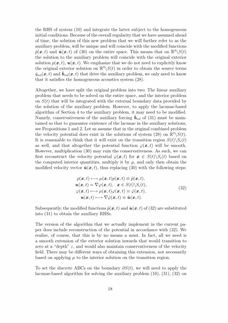
Fig. 2. Grid convergence study with lacunae-based ABCs, ε = 10∆r.

all three grids that we have employed. The total integration time was 100dc,

i.e., one hundred times the interval required for the waves to cross the domain.The error was evaluated in the maximum norm on the domain S(t). We seethat the algorithm provides for no long-term error buildup, and also that itdisplays the design second-order grid convergence. The oscillations in the errorprofiles on Figure 2 have the period of 10 time units, and apparently followthe acceleration/deceleration cycles of the source motion. Error profiles forthe velocity components u and w look similarly and we do not present them.

We should mention that the error curves on Figure 2 were obtained for a rela-tively wide transition region S(t)\Sε(t), on the order of ten grid cell sizes. Eventhough the actual width of this region decreases with the refinement of thegrid, the issue of how the width ε affects the algorithm performance deservesto be thoroughly addressed. From the numerical standpoint, the width of thetransition region determines how well the smooth function µ(x , t) is resolvedon the grid, and as such, how smooth the auxiliary RHSs will effectively be.The latter, in turn, affect the quality of the discrete lacunae, i.e., how sharpthe aft fronts of the waves really are in the discrete framework. This is im-portant because every time a retarded component is subtracted, see (27), weassume that what is being subtracted inside the lacuna, i.e., on the domainS(t), is zero, or more precisely, a small quantity that converges to zero withthe refinement of the grid; the convergence, however, hinges on the smoothnessof the source terms. Besides having a potential effect on the error behavior,

27

the width of the transition region also determines on how many grid nodes theauxiliary RHSs are supported. We remind that those RHSs basically controlthe extent of temporal nonlocality of the lacunae-based ABCs. The algorithmrequires keeping them on the interval of length Tint, and as such, the morenarrow the transition region is, the less additional storage is needed.

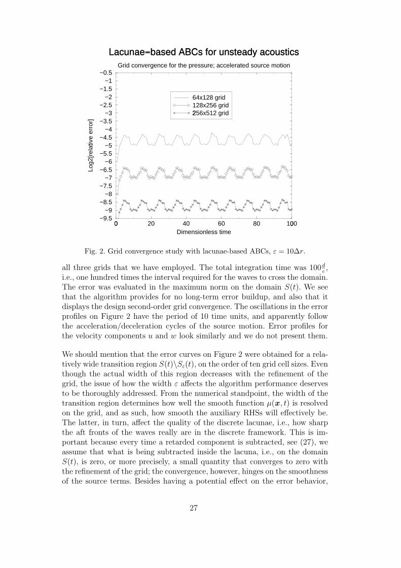
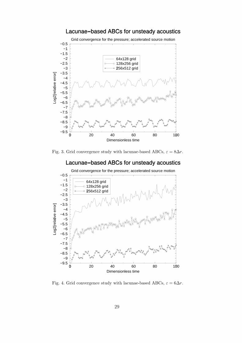
In Figures 3, 4, 5, and 6 we are showing similar pressure error profiles for thewidth of the transition region ε = 8, 6, 4, and 2 grid cell sizes, respectively.

We observe that with the decrease of ε the error behavior deteriorates, whichis natural to expect. We also notice, though, that the deterioration is morevisible on the coarser grids, whereas on the finest 256 × 512 grid it is muchslower. The 256×512 error profile is still practically flat for ε = 8, see Figure 3,and it loses only one binary order of magnitude for ε = 6 over the entire longinterval of integration, see Figure 4. Even for a rather narrow transition region,ε = 4, see Figure 5, the finest grid error only grows by less than a factor of2 over the first half of the integration interval, which is still fifty times thetime needed for the waves to cross the domain. The rates of error increasebecome practically equal on all grids only for the narrowest transition regionthat we have tried: ε = 2, see Figure 6. Having only two grid cells in thetransition region basically implies that there is no smoothing at all, rathera sharp truncation, and instead of µ(x , t) we are using an equivalent of theHeaviside function on the grid. But even in this case we can see that the initialjump of the error is much smaller on the fine grid than on the coarser grids.

As of yet, we cannot offer a rigorous theoretical explanation of why the algo-rithm appears more sensitive to the quality of the discrete lacunae on coarsergrids than on the fine grid. We can only qualitatively suggest that it has todo with the actual magnitude of those discrete “tails” behind the aft frontsof the waves that are due to the “imperfections” in the auxiliary sources, andthat apparently are still smaller on fine grids. Altogether, this phenomenonis certainly beneficial, because fine grids are needed for high overall accuracyanyway, and at the same time they will allow to maintain high accuracy ofthe boundary treatment for longer periods of time. We should also note thatfor many practical applications the actual integration times will likely be notas long as those that we have used for the current proof-of-concept. This willleave even less room for the error buildup due to the boundary treatment.

7 Conclusions

We have constructed and tested the algorithm for setting highly-accurateglobal artificial boundary conditions for the computation of time-dependentacoustic waves. This work is an extension of our previous approach that applied

28

0�

20 40 60 80 100�

Dimensionless time

−9.5−9

−8.5−8

−7.5−7

−6.5−6

−5.5−5

−4.5−4

−3.5−3

−2.5−2

−1.5−1

−0.5

Log2

[rel

ativ

e er

ror]

�

Lacunae−based ABCs for unsteady acousticsGrid convergence for the pressure; accelerated source motion

64x128 grid128x256 grid256x512 grid

�

Fig. 3. Grid convergence study with lacunae-based ABCs, ε = 8∆r.

0�

20 40 60 80 100�

Dimensionless time

−9.5−9

−8.5−8

−7.5−7

−6.5−6

−5.5−5

−4.5−4

−3.5−3

−2.5−2

−1.5−1

−0.5

Log2

[rel

ativ

e er

ror]

�

Lacunae−based ABCs for unsteady acousticsGrid convergence for the pressure; accelerated source motion

64x128 grid128x256 grid256x512 grid

�

Fig. 4. Grid convergence study with lacunae-based ABCs, ε = 6∆r.

29

0�

20 40 60 80 100�

Dimensionless time

−9.5−9

−8.5−8

−7.5−7

−6.5−6

−5.5−5

−4.5−4

−3.5−3

−2.5−2

−1.5−1

−0.5

Log2

[rel

ativ

e er

ror]

�

Lacunae−based ABCs for unsteady acousticsGrid convergence for the pressure; accelerated source motion

64x128 grid128x256 grid256x512 grid

�

Fig. 5. Grid convergence study with lacunae-based ABCs, ε = 4∆r.

0�

20 40 60 80 100�

Dimensionless time

−9.5−9

−8.5−8

−7.5−7

−6.5−6

−5.5−5

−4.5−4

−3.5−3

−2.5−2

−1.5−1

−0.5

Log2

[rel

ativ

e er

ror]

�

Lacunae−based ABCs for unsteady acousticsGrid convergence for the pressure; accelerated source motion

64x128 grid128x256 grid256x512 grid

�

Fig. 6. Grid convergence study with lacunae-based ABCs, ε = 2∆r.

30

to the scalar wave equation [13]. The algorithm is based on the presence of lacu-nae (aft fronts of the waves) in the three-dimensional wave-type solutions. TheABCs are obtained directly for the discrete formulation of the problem andcan complement any consistent and stable finite-difference scheme. In so doing,neither a rational approximation of non-reflecting kernels, nor discretization ofthe continuous boundary conditions is required. The extent of temporal non-locality of the new ABCs appears fixed and limited, and this is not a result ofany approximation but rather a direct consequence of the fundamental prop-erties of the solution. The proposed ABCs can handle artificial boundaries ofirregular shape on regular grids with no fitting/adaptation needed. Besides,they possess a unique capability of being able to handle boundaries of movingcomputational domains, including the case of accelerated motion.

For the case of an acoustic source engaged in an accelerated motion, we haveconducted numerical experiments that corroborate the theoretical design prop-erties of the algorithm. We are currently unaware of any other acoustic ABCs’algorithm in the literature with the capability of handling the acceleratedmotion. We have also shown experimentally that when a key parameter thatcharacterizes the algorithm changes so that to reduce the overall memory re-quirements, the performance of the ABCs suffers in an expected way. However,the deterioration of the long-term performance on fine grids is much slowerthan that on coarse grids.

Finally, we should mention that even though the full description of the algo-rithm provided in the paper does address a number of technical issues, its keyidea is most straightforward. In one sentence it can be formulated as follows:One should not continue the computation inside the lacuna once the solu-tion has become zero there due to “natural causes.” Otherwise the error mayunwarrantably build up on one hand, and on the other hand, the extent ofthe required temporal pre-history of the solution may grow un-justifiably high.The technical issues that we have discussed relate primarily to what to do withthe waves outside, and not inside, the domain of interest. In the framework ofthe previous analysis, we simply allow them to propagate a certain distanceaway till they get reflected, and then set up the auxiliary domain so that thereflected waves do not reach the domain of interest before it completely fallsinside the lacuna. This, however, is by no means the only possible option. Infact, any treatment of the outgoing waves that would prevent the reflectionsfrom re-entering the domain of interest before it falls into the lacuna will beappropriate. At the same time, introducing an alternative to the approachdescribed in the current paper may be beneficial from the standpoint of theoverall computational cost. For example, a treatment of the sponge layer typethat slows down the outgoing waves, see, e.g., [25,26], may allow to reduce thesize of the auxiliary domain. Alternatively, the lacunae-based approach canbe combined with a PML-based treatment for the waves outside the domainof interest, see, e.g., the survey papers [27, 28]. In any event, linearity has

31

to be maintained, otherwise it will not be possible to partition the problemsimilarly to (16), (18), (19). These combined approaches will be subject of afuture study.

Acknowledgements

The author is very thankful to the reviewers of the paper for their helpfulcomments.

References

[1] D. Givoli, Non-reflecting boundary conditions, J. Comput. Phys. 94 (1991) 1–29.

[2] T. Hagstrom, Radiation boundary conditions for the numerical simulation ofwaves, in: A. Iserlis (Ed.), Acta Numerica, Vol. 8, Cambridge University Press,Cambridge, 1999, pp. 47–106.

[3] S. V. Tsynkov, Numerical solution of problems on unbounded domains. Areview, Appl. Numer. Math. 27 (1998) 465–532.

[4] M. J. Grote, J. B. Keller, On nonreflecting boundary conditions, J. Comput.Phys. 122 (1995) 231–243.

[5] M. J. Grote, J. B. Keller, Exact nonreflecting boundary conditions for the time-dependent wave equation, SIAM J. Appl. Math. 55 (1995) 280–297.

[6] M. J. Grote, J. B. Keller, Nonreflecting boundary conditions for time-dependentscattering, J. Comput. Phys. 127 (1996) 52–65.

[7] I. L. Sofronov, Artificial boundary conditions of absolute transparency for two-and three-dimensional external time-dependent scattering problems, EuropeanJ. Appl. Math. 9 (1998) 561–588.

[8] I. L. Sofronov, Non-reflecting inflow and outflow in a wind tunnel for transonictime-accurate simulations, J. Math. Anal. Appl. 221 (1998) 92–115.

[9] B. Alpert, L. Greengard, T. Hagstrom, Rapid evaluation of nonreflectingboundary kernels for time-domain wave propagation, SIAM J. Numer. Anal.37 (2000) 1138–1164.

[10] B. Alpert, L. Greengard, T. Hagstrom, Nonreflecting boundary conditions forthe time-dependent wave equation, J. Comput. Phys. 180 (1) (2002) 270–296.

[11] E. Michielssen, A. Ergin, B. Shanker, D. Weile, The multilevel plane wave timedomain algorithm and its applications to the rapid solution of electromagnetic

32

scattering problems: A review, in: Mathematical and numerical aspects of wavepropagation (Santiago de Compostela, 2000), SIAM, Philadelphia, PA, 2000,pp. 24–33.

[12] V. S. Ryaben’kii, S. V. Tsynkov, V. I. Turchaninov, Long-time numericalcomputation of wave-type solutions driven by moving sources, Appl. Numer.Math. 38 (2001) 187–222.

[13] V. S. Ryaben’kii, S. V. Tsynkov, V. I. Turchaninov, Global discrete artificialboundary conditions for time-dependent wave propagation, J. Comput. Phys.174 (2) (2001) 712–758.

[14] V. S. Ryaben’kii, Nonreflecting time-dependent boundary conditions onartificial boundaries of varying location and shape, Appl. Numer. Math. 33(2000) 481–492.

[15] V. S. Vladimirov, Equations of Mathematical Physics, Dekker, New-York, 1971.

[16] I. Petrowsky, On the diffusion of waves and the lacunas for hyperbolic equations,Matematicheskii Sbornik (Recueil Mathematique) 17 (59) (3) (1945) 289–370.

[17] R. Courant, D. Hilbert, Methods of Mathematical Physics. Volume II, Wiley,New York, 1962.

[18] L. D. Landau, E. M. Lifshitz, Fluid Mechanics, Pergamon Press, Oxford, 1986.

[19] C. L. Morfey, Dictionary of Acoustics, Academic Press, San Diego, 2001.

[20] L. Ting, M. J. Miksis, Exact boundary conditions for scattering problems, J.Acoust. Soc. Am. 80 (1986) 1825–1827.

[21] D. Givoli, D. Cohen, Nonreflecting boundary conditions based on Kirchhoff-typeformulae, J. Comput. Phys. 117 (1995) 102–113.

[22] S. V. Tsynkov, External boundary conditions for three-dimensional problemsof computational aerodynamics, SIAM J. Sci. Comp. 21 (1999) 166–206.

[23] P. M. Morse, H. Feshbach, Methods of Theoretical Physics. Parts I and II,McGraw-Hill, Boston, 1953.

[24] K. S. Yee, Numerical solution of initial boundary value problem involvingMaxwell’s equations in isotropic media, IEEE Trans. Antennas Propagat. 14(1966) 302–307.

[25] M. Israeli, S. Orszag, Approximation of radiation boundary conditions, J.Comput. Phys 41 (1981) 115–135.

[26] S. Karni, Far-field filtering operators for suppression of reflections from artificialboundaries, SIAM J. Numer. Anal. 33 (1996) 1014–1047.

[27] S. Abarbanel, D. Gottlieb, On the construction and analysis of absorbing layersin CEM, Appl. Numer. Math. 27 (1998) 331–340.

[28] E. Turkel, A. Yefet, Absorbing PML boundary layers for wave-like equations,Appl. Numer. Math. 27 (1998) 533–557.

33