Numerical and Experimental Determination of Boundary Layer Thickness

MEHMET ARDICLIOGLU, OZGUR OZTURK Department of Civil Engineering,

Erciyes University Faculty of Engineering, 38039, Kayseri

TURKEY

Abstract: - In this paper, boundary layer development was investigated for smooth open channel flow. For this purpose ADV velocity measurements were made at 16 different distances along the channel mid section for four different flow conditions. Both experimental and theoretical methods implemented in the computation of boundary layer thickness. Boundary layer thicknesses were determined using Matlab codes which work based on the von Karman integral momentum method. Theoretical method gives high boundary layer thickness and small boundary layer development length values. The boundary layer development varies between 30 to 65 times of the water depth for all flow conditions. Key-Words: - Open channel flow, Boundary layer thickness and development, Power law 1 Introduction Boundary layer is the region near a solid where the fluid motion is affected by the solid boundary. The details of the flow within the boundary layer are very important for many problems in aerodynamics, including the development of a wing stall, the skin friction drag of an object, the heat transfer that occurs in high speed flight, and the performance of a high speed aircraft inlet [1]. The fluid in direct contact with the body surface adheres to the surface and has zero velocity. The fluid just above the surface is slowed by frictional forces associated with the viscosity of the fluid. The closer the fluid is to the surface, the more it is slowed. The result is a thin layer where the horizontal velocity, u, of the fluid increases from zero at the body surface to a velocity close to V. The shapes of the boundary layer profiles above a particular position on a surface depend on the shape of the body, surface roughness, the upstream history of the boundary layer, the surrounding flow field and Reynolds number. Flow in the boundary layer can be laminar or turbulent, resulting in radically different classes of profile shapes. Prandtl (1952), Schlichting (1979) and Batchelor (1967) provide thorough descriptions of the boundary layer concept [2].

In this study we try to determine boundary layer thickness and development length both experimentally and theoretically using von Karman integral momentum method. 2 Determination of Boundary Layer

Thickness Boundary layer thickness, δ, can be defined as that distance from the wall where the velocity differs by one percent from the free surface velocity. Boundary layer thickness and development length could be determined using both experimental and numerical methods. In the experimental method velocity distributions along the channel mid section are measured to determine the boundary layer thickness when velocity distribution reaches free surface velocity. The developed flow occurs when the velocity profile along the channel length is constant.

Boundary layer thickness could be determined using theoretically by the von Karman integral momentum method. Momentum equation for turbulence boundary layer flow over smooth surface could be given with Eq. (1) [1].

⎥⎦

⎤⎢⎣

⎡⎟⎠⎞

⎜⎝⎛ −ρ

∂∂

=τ ∫δ

0

20 dz

Vu1

VuV

x (1)

Proceedings of the 5th WSEAS International Conference on Applications of Electrical Engineering, Prague, Czech Republic, March 12-14, 2006 (pp167-170)

Prandtl [3] defined power law for velocity distribution using Blasius friction factors equation. Later on this equation is improved for the changing values of Reynolds number and expressed as given in Eq. (2).

n/1*

*

zuCuu

⎟⎠⎞

⎜⎝⎛υ

= (2)

in which u is the velocity in the longitudinal direction, u* is the friction velocity, z is the distance from the bed anf C, n are constants.

Kandula et all. [4] introduced that the Eq. (2) could be used for turbulent open channel flow. In the experimental measurements, the constants in the Eq. (2) are found as (C=8.3, n=7) and (C=8.41, n=6.8) by Kandula et all. and Ardiclioglu [5], respectively. In Eq. (2) boundary condition written as z=δ, u=V and

n/1*

*

uCuV

⎟⎠⎞

⎜⎝⎛υδ

= (3)

When Eq. (2) is divided to Eq. (3), velocity equation could be rewritten as given in Eq. (4).

n/1zVu

⎟⎠⎞

⎜⎝⎛δ

= (4)

Eq. (1) is solved using Eq. (4) and the following Eq. (5) is obtained as:

( )( ) dxdV

2n1nn 2

0δ

ρ++

=τ (5)

On the other hand, if shear velocity in Eq. (3) is written as ρτ= /u 0* , 0τ is obtained as given in Eq. (6).

( )

( )n1/22

1n/n20 VV

C1 +

+ ⎟⎠⎞

⎜⎝⎛

δυ

ρ=τ (6)

As can be seen, left sides of both Eq (5) and (6) refer to same 0τ value and, therefore, right sides of them are equal. This provides us the boundary layer thickness which is given in Eq. (7).

( )( )

( )( )( )

dxV2n1n/n

C/1dn1/21n/n2

1n/2++

+ ⎟⎠⎞

⎜⎝⎛ υ

++=δδ (7)

Eq. (7) could be solved using boundary condition to determine the boundary layer thickness.

3. Experiments Experiments were carried out at hydraulic laboratory of the Erciyes University, Kayseri, Turkey. The glass-walled laboratory channel was 9.0m long, 0.6m wide and 0.6m deep. The channel bed was covered with a glass layer, which was thought suitable for smooth-wall experiments. Flow rates were measured using a Krohne UL 600R type ultrasonic flowmeter and flow velocities were measured by a Acoustic Doppler Velocimeter (ADV) produced by Sontek which is a versatile, high-precision and measures all three flow velocity components. Experiments were conducted for 4 different subcritical uniform flow conditions. The details of the test conditions are given in Table 1 in which Q is the discharge, h is the flow depth, Re(=4VR/υ) is the Reynolds number, Fr(= gh/V ) is the Froude number, V is the average velocity of the flow, R is the hydraulic radius and υ is the kinematics viscosity of water. Flow velocities were measured at 16 mid verticals (x=0.5, 1.0, 1.5, 2.0, .....…, 8.0m). along the flow developing zone.

Table 1. Details of Experimental Conditions

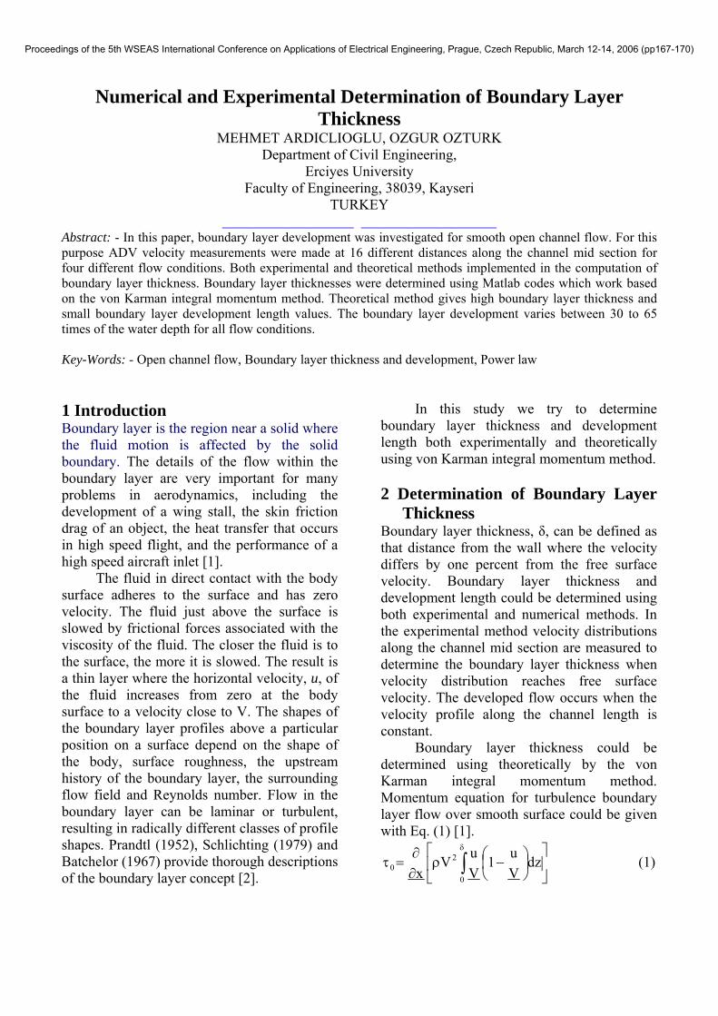
4. Results and Analysis All measured velocity profiles for four tests are determined. Fig.1 shows the measured velocity profiles for Test 2 and gives the velocity profiles along the centerline of the developing flow. By examining the velocity profiles in Fig.1, it may be seen that the vertical distribution of the velocities remains almost unchanged and consequently the flow can be assumed fully developed when x≥450 cm for Test 2. That is the length of the boundary layer development is L=450 cm for this particular case.

Test Q (lt/sn )

h (cm)

Re Fr Lmeas(cm)

Ltheo (cm)

1 10.08 6.19 48879 0.35 400 250 2 20.05 9.68 88648 0.35 450 350 3 30.19 11.64 127176 0.40 550 400 4 37.28 14.14 148173 0.37 600 450

Proceedings of the 5th WSEAS International Conference on Applications of Electrical Engineering, Prague, Czech Republic, March 12-14, 2006 (pp167-170)

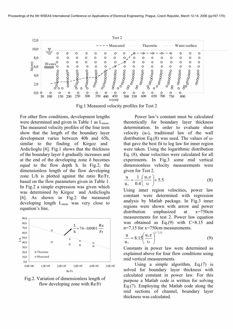
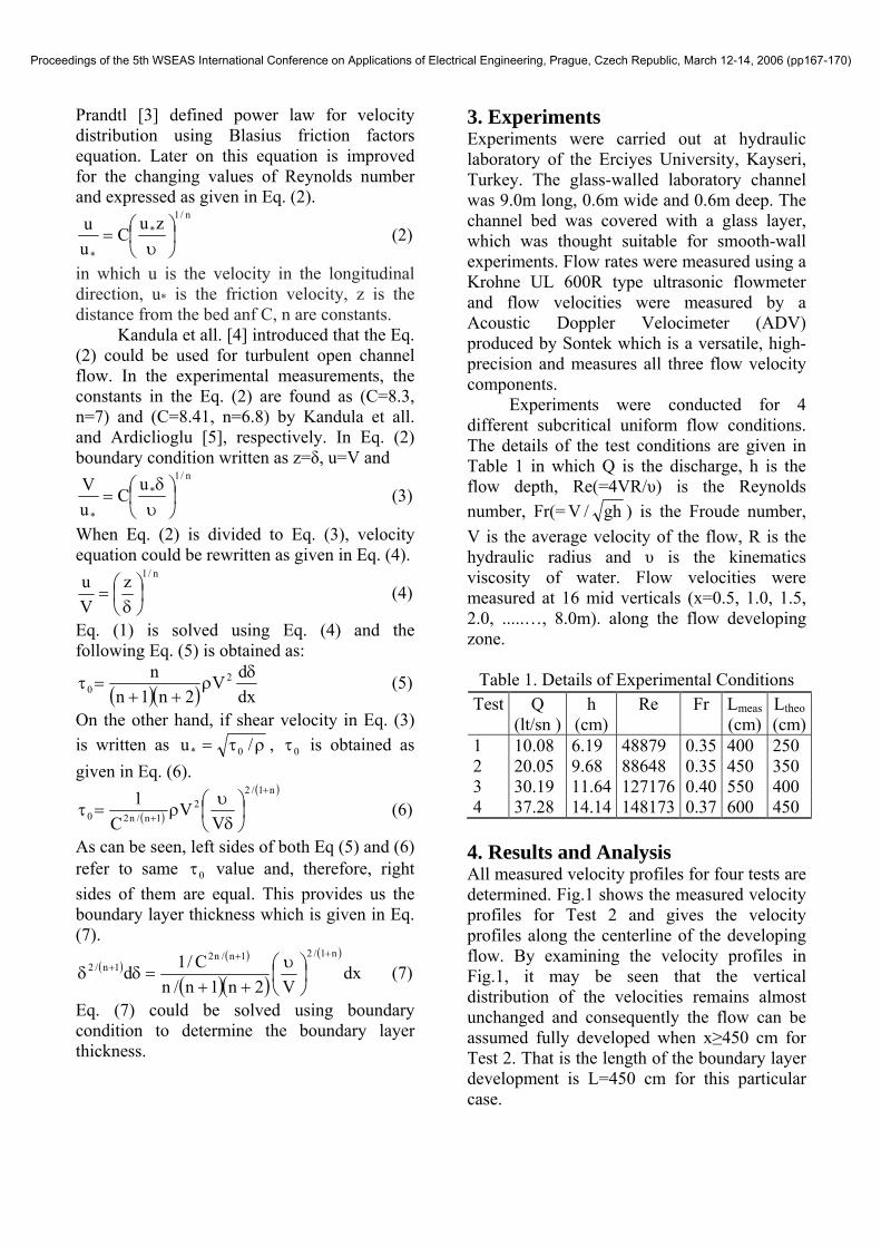
Fig.1 Measured velocity profiles for Test 2 For other flow conditions, development lengths were determined and given in Table 1 as Lmeas. The measured velocity profiles of the four tests show that the length of the boundary layer development varies between 40h and 65h, similar to the finding of Kirgoz and Ardiclioglu [6]. Fig.1 shows that the thickness of the boundary layer δ gradually increases and at the end of the developing zone δ becomes equal to the flow depth h. In Fig.2, the dimensionless length of the flow developing zone L/h is plotted against the ratio Re/Fr, based on the flow parameters given in Table 1. In Fig.2 a simple expression was given which was determined by Kirgoz and Ardiclioglu [6]. As shown in Fig.2 the measured developing length Lmeas was very close to equation’s line.

Fig.2. Variation of dimensionless length of flow developing zone with Re/Fr

Power law’s constant must be calculated theoretically for boundary layer thickness determination. In order to evaluate shear velocity (u*), traditional law of the wall distribution Eq.(8) was used. The values of u* that gave the best fit to log law for inner region were taken. Using the logarithmic distribution Eq. (8), shear velocities were calculated for all experiments. In Fig.3 some mid vertical dimensionless velocity measurements were given for Test 2.

5.5zu4.0

1uu *

*

+⎟⎠⎞

⎜⎝⎛υ

= (8)

Using inner region velocities, power law constant were determined with regression analysis by Matlab package. In Fig.3 inner regions were shown with arrow and power distribution emphasized at x=750cm measurements for test 2. Power law equation was obtained as Eq.(9) with C=8.15 and n=7.15 for x=750cm measurements.

15.7/1*

*

zu15.8uu

⎟⎠⎞

⎜⎝⎛υ

= (9)

Constants in power law were determined as explained above for four flow conditions using mid vertical measurements. Using a simple algorithm, Eq.(7) is solved for boundary layer thickness with calculated constant in power law. For this purpose a Matlab code is written for solving Eq.(7). Employing the Matlab code along the mid sections of channel, boundary layer thickness was calculated.

0,0

10,020,0

30,0

40,050,0

60,0

70,080,0

90,0

0,0E+00 1,0E+05 2,0E+05 3,0E+05 4,0E+05 5,0E+05

Re/Fr

L/h

TheoreticMeasured

FrRe

0001.076hL

−=

Test 2

0,0

2,0

4,0

6,0

8,0

10,0

12,0

x (cm)

h(cm

)

Measured Theoretic Water surface

50 600100 550150 200 250 800350300 500450400 750700650

20 cm/s

Proceedings of the 5th WSEAS International Conference on Applications of Electrical Engineering, Prague, Czech Republic, March 12-14, 2006 (pp167-170)

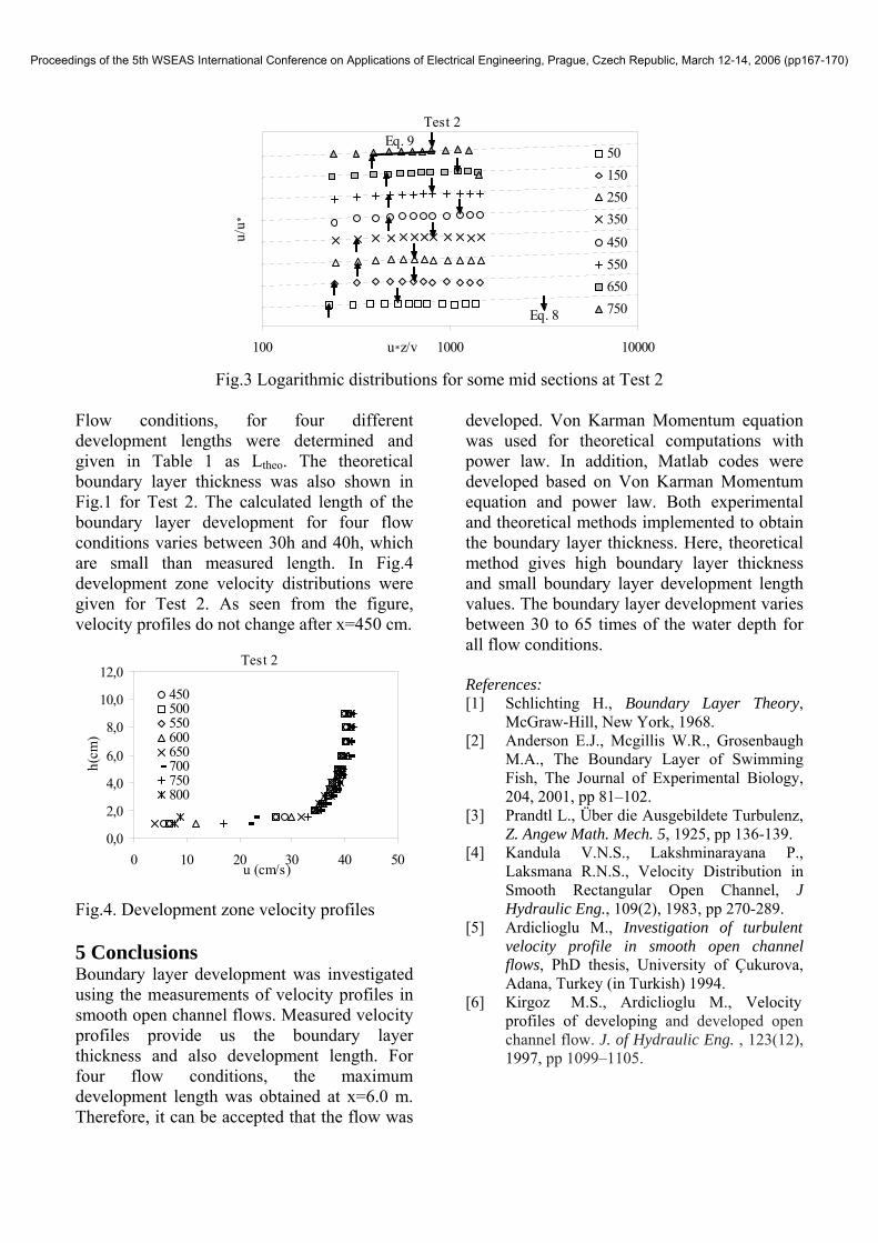
Fig.3 Logarithmic distributions for some mid sections at Test 2 Flow conditions, for four different development lengths were determined and given in Table 1 as Ltheo. The theoretical boundary layer thickness was also shown in Fig.1 for Test 2. The calculated length of the boundary layer development for four flow conditions varies between 30h and 40h, which are small than measured length. In Fig.4 development zone velocity distributions were given for Test 2. As seen from the figure, velocity profiles do not change after x=450 cm. Fig.4. Development zone velocity profiles 5 Conclusions Boundary layer development was investigated using the measurements of velocity profiles in smooth open channel flows. Measured velocity profiles provide us the boundary layer thickness and also development length. For four flow conditions, the maximum development length was obtained at x=6.0 m. Therefore, it can be accepted that the flow was

developed. Von Karman Momentum equation was used for theoretical computations with power law. In addition, Matlab codes were developed based on Von Karman Momentum equation and power law. Both experimental and theoretical methods implemented to obtain the boundary layer thickness. Here, theoretical method gives high boundary layer thickness and small boundary layer development length values. The boundary layer development varies between 30 to 65 times of the water depth for all flow conditions. References: [1] Schlichting H., Boundary Layer Theory,

McGraw-Hill, New York, 1968. [2] Anderson E.J., Mcgillis W.R., Grosenbaugh

M.A., The Boundary Layer of Swimming Fish, The Journal of Experimental Biology, 204, 2001, pp 81–102.

[3] Prandtl L., Über die Ausgebildete Turbulenz, Z. Angew Math. Mech. 5, 1925, pp 136-139.

[4] Kandula V.N.S., Lakshminarayana P., Laksmana R.N.S., Velocity Distribution in Smooth Rectangular Open Channel, J Hydraulic Eng., 109(2), 1983, pp 270-289.

[5] Ardiclioglu M., Investigation of turbulent velocity profile in smooth open channel flows, PhD thesis, University of Çukurova, Adana, Turkey (in Turkish) 1994.

[6] Kirgoz M.S., Ardiclioglu M., Velocity profiles of developing and developed open channel flow. J. of Hydraulic Eng. , 123(12), 1997, pp 1099–1105.

Test 2

0,0

2,0

4,0

6,0

8,0

10,0

12,0

0 10 20 30 40 50u (cm/s)

h(cm

)

450500550600650700750800

Test 2

100 1000 10000u*z/v

u/u*

50150250350450550650750Eq. 8

Eq. 9

Proceedings of the 5th WSEAS International Conference on Applications of Electrical Engineering, Prague, Czech Republic, March 12-14, 2006 (pp167-170)