numerical and reliability analysis of gravity …
TRANSCRIPT

Clemson UniversityTigerPrints
All Theses Theses
8-2012
NUMERICAL AND RELIABILITY ANALYSISOF GRAVITY CANTILEVER RETAININGWALLS BACKFILLED WITH SHREDDEDTIRES SUBJECTED TO SEISMIC LOADSEleanor HugginsClemson University, [email protected]
Follow this and additional works at: https://tigerprints.clemson.edu/all_theses
Part of the Civil Engineering Commons
This Thesis is brought to you for free and open access by the Theses at TigerPrints. It has been accepted for inclusion in All Theses by an authorizedadministrator of TigerPrints. For more information, please contact [email protected].
Recommended CitationHuggins, Eleanor, "NUMERICAL AND RELIABILITY ANALYSIS OF GRAVITY CANTILEVER RETAINING WALLSBACKFILLED WITH SHREDDED TIRES SUBJECTED TO SEISMIC LOADS" (2012). All Theses. 1437.https://tigerprints.clemson.edu/all_theses/1437

TITLE PAGE
NUMERICAL AND RELIABILITY ANALYSIS OF GRAVITY CANTI LEVER RETAINING WALLS BACKFILLED WITH SHREDDED
TIRES SUBJECTED TO SEISMIC LOADS
A Thesis Presented to
the Graduate School of Clemson University
In Partial Fulfillment of the Requirements for the Degree
Master of Science Civil Engineering
by Eleanor Lynn Huggins
August, 2012
Accepted by: Nadarajah Ravichandran, PhD, Committee Chair
Hsein Juang, PhD, PE Bradley Putman, PhD

ii
ABSTRACT
Shredded tires have been considered as a suitable alternative to conventional sand
and gravel backfill materials as they offer benefits from their significantly lower unit
weight, reductions in the cost of materials and construction, and because they utilize a
common and potentially hazardous waste material. This research addresses some gaps in
previous research in the implementation of shredded tires in this capacity by examining
variation in material properties through a reliability analysis, developing an improved
design technique for retaining walls tailored to shredded tire fills, and simulating how
shredded tire backfill behaves in conjunction with retaining walls when subject to seismic
loads. First, an in depth literature review was performed to determine previously defined
material properties of shredded tires based on a myriad of standard and specialized lab
tests performed for many sizes and types of shredded tires. Review of the literature also
served to identify additional design considerations that, along with geotechnical
properties and LRFD methods, were used to design a retaining wall that was optimized
for use with shredded tire fills. This wall was then modeled with the shredded tire fill in
the finite element software, PLAXIS, under seismic loadings and considering variations
in the material properties as defined by the literature as well as utilizing different
damping schemes at governing equation level and constitutive model for the materials.
The conclusion was that shredded tires can be a very beneficial alternative to
conventional fills and further benefit can be realized by designing walls specifically for
shredded tire use thus reducing wall size and changing wall dimensions for optimum
shredded tire fill performance.

iii
DEDICATION
I dedicate this thesis to my parents for teaching me everything I’ve ever known about life
and to all the people who have taught me everything else.

iv
ACKNOWLEDGEMENTS
I would first like to thank my advisor, Dr. Nadarajah Ravichandran for his
invaluable guidance and support throughout the research process. He taught me how to
be a successful researcher and the importance of quality and attention to detail in my
work as well as honing my skills as a geotechnical engineer in the process. He was in
many ways enough opposite of me in thinking so as to be a great catalyst for creative and
critical thought and I can only hope that this work reflects our collective efforts and all
that he taught me. I also want to thank my committee members, Dr. Bradley Putman and
Dr. Hsein Juang. Each has shaped my education both inside the classroom and out and
has shown me a great deal of support. They too brought some great and varied ideas to
the project and made the work more comprehensive and widely applicable through their
unique expertise and point of view.
I would also like to acknowledge the undergraduate students that took on the, at
times, thankless task of working on research. First is Andrew Brownlow, who worked on
PLAXIS with me and helped take the burden off of me in running simulations and
processing the mountains of data that sometimes accompanied the project. Second is
Daniel Kyser who helped with lab work on additional research fronts. All I can hope is
that these two learned a little something from me and I wish them great success in their
further ventures and educational exploits.
Finally this research and my graduate education as a whole would not have been
possible without the Aniket Shrikhande Memorial Assistantship. I thank the Shrikhande
family for their support and for making my work possible.

v
TABLE OF CONTENTS
TITLE PAGE ....................................................................................................................... i
ABSTRACT ........................................................................................................................ ii
DEDICATION ................................................................................................................... iii
ACKNOWLEDGEMENTS ............................................................................................... iv
TABLE OF CONTENTS .................................................................................................... v
LIST OF TABLES ........................................................................................................... viii
LIST OF FIGURES ........................................................................................................... ix
CHAPTER
I. INTRODUCTION ............................................................................................ 1
Thesis Organization .................................................................................... 2
II. LITERATURE REVIEW ................................................................................. 4
Shredded Tire Material Property Tests ....................................................... 4
Safety and Environmental Concerns ......................................................... 12
Economics ................................................................................................. 20
III. MODEL BASIS AND RETAINING WALL DESIGN ................................. 23
Problem Overview .................................................................................... 23
Retaining Wall Design Process ................................................................. 24

vi
IV. FINITE ELEMENT MODELING METHODS.............................................. 29
Selection of Appropriate Finite Element Mesh ........................................ 30
Selection of Appropriated Finite Element Domain .................................. 34
Final Finite Element Model ...................................................................... 36
V. DAMPING AND MATERIAL MODELING ................................................ 38
Rayleigh Damping .................................................................................... 39
The Mohr-Coulomb Material Model ........................................................ 41
The Hardening Soil Model........................................................................ 43
VI. DETERMINATION OF MODEL INPUT PARAMETERS .......................... 46
Determination of the Mohr-Coulomb Parameters .................................... 46
Calibration of the Hardening Soil Model.................................................. 48
Calibration to Available Experimental Data .......................................... 51
Calibration of Parametric Study Parameters .......................................... 55
Material Properties and Input Parameters ................................................. 57
VII. RESULTS AND DISCUSSION ..................................................................... 61
Comparison with Standard Backfill .......................................................... 61
Parametric Study on Variations in Shredded Tire Properties ................... 69
Reliability Analysis of Parametric Study Results ..................................... 74

vii
VIII. EFFECTS OF CONSTITUATIVE MODELS ON COMPUTED
RESPONSES .................................................................................................. 79
Variation in Response Due to Material Model and Damping ................... 79
Mohr-Coulomb Model without Rayleigh Damping ................................. 84
Mohr-Coulomb Model with Rayleigh Damping....................................... 89
IX. CONCLUSIONS AND FUTURE WORK ..................................................... 94
Conclusions ............................................................................................... 94
Practical Application of this Research ...................................................... 96
Recommendations for Future Work.......................................................... 96
APPENDICES .................................................................................................................. 99
A. Worksheets Demonstrating Static Wall Design Methods ................................... 100
B. Worksheets Demonstrating Seismic Wall Design Methods ............................... 105
C. Full Review of Shredded Tire Properties from the Literature ............................ 111
REFERENCES ............................................................................................................... 112

viii
LIST OF TABLES
Table Page
3.1 Comparison of Material Requirements for Shredded Tires
and Conventional Sand Backfills ........................................................... 26
3.2. Properties of the plates comprising the retaining
structure, per unit length ........................................................................ 28
6.1. Properties of shredded tires gained from the literature ................................ 47
6.2. Parameter Definitions for the Hardening Soil Model in PLAXIS ............... 49
6.3. Properties for all materials for use in the Hardening Soil Model ................ 58
6.4. Properties for all materials for use in the Mohr-Coulomb Model ............... 59
6.5. Rayleigh Damping Coefficients for Soils .................................................... 60
7.1. Comparison of Maximum Responses for Sand and Shredded
Tire Backfills ......................................................................................... 65
7.2. Summary of results from parametric study .................................................. 72
7.3. Reliability analysis of data from the parametric study ................................ 76
8.1. Summary of results from parametric study: Undamped
M-C Model............................................................................................. 87
8.2. Summary of results from parametric study: Damped
M-C Model............................................................................................. 91

ix
LIST OF FIGURES
Figure Page
3.1. A sketch of the problem being considered .................................................. 23
3.2. Finite element mesh used in all studies....................................................... 25
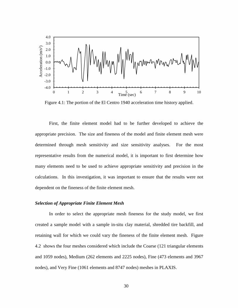
4.1. The portion of the El Centro 1940 acceleration time history
applied .................................................................................................... 30
4.2. Mesh fineness options observed in PLAXIS ............................................... 32
4.3. Displacement time history for the retaining wall tip for each
mesh fineness ........................................................................................ 33
4.4. The shear and bending moment distributions in the retaining
wall at the end of dynamic loading for each mesh fineness .................. 33
4.5. Mesh showing variation lengths A and B for size sensitivity study ............ 34
4.6. Displacement time history for the retaining wall tip for each
model size .............................................................................................. 35
4.7. The shear and bending moment distributions in the retaining wall at
the end of dynamic loading for each model size .................................... 36
4.8. Finite element mesh used in all studies........................................................ 37
5.1. Mohr-Coulomb Stress-Strain Criterion based on PLAXIS input
parameters .............................................................................................. 42

x
List of Figures (Continued) Figure Page
5.2. Hardening Soil Model Stress-Strain Criteria based on PLAXIS
input parameters ..................................................................................... 44
6.1. Graphical calibration of Hardening Soil Model to experimental
data and Mohr Coulomb criterion from two sources and
four confining pressures ......................................................................... 53
6.2. Calibration of Hardening Soil Model for the variations in the
Friction Angle ........................................................................................ 56
6.3. Calibration of Hardening Soil Model for the variations in the
Cohesion ................................................................................................ 57
7.1. Wall Deflection Time Histories for Sand and Shredded Tire
Backfills ................................................................................................. 62
7.2. Maximum Shear Envelopes for Sand and Shredded Tire Fills .................... 63
7.3. Maximum Shear Envelopes for Sand and Shredded Tire Fills .................. 64
7.4. Spectral Accelerations observed by location considering 5%
Damping ................................................................................................. 67
7.5. Deflection time histories of the wall stem for variation of
each tire material property: HS Model-Damped .................................... 70
7.6. Variation in maximum load from material property variations ................... 73

xi
List of Figures (Continued) Figure Page
8.1. Comparisons of Acceleration Responses for HS Model and
MC Models ............................................................................................ 80
8.2. Spectral Accelerations by location observed considering 5%
Damping ................................................................................................. 83
8.3. Deflection time histories of the wall stem for variation of each
tire material property: Undamped M-C Model ...................................... 84
8.4. Variation in maximum wall load based on material property
variations: Undamped M-C Model ........................................................ 88
8.5. Deflection time histories of the wall stem for variation of each
tire material property: Damped M-C Model .......................................... 90
8.6. Variation in maximum wall load based on material property
variations: Damped M-C Model ............................................................ 92

1
CHAPTER 1
INTRODUCTION
As resources become more and more scarce and waste becomes a more and more
pervasive problem, the reality of how the cradle-to-grave system can be destructive to
society becomes more and more glaring. One example of such a problem is in the
disposal of waste tires. In the United States alone, between 200 million and 300 million
waste tires are generated each year and disposing of these tires is becoming an
increasingly great burden on society. Whole tires when disposed of in dump sites or
dumped illegally provide a breeding ground for harmful mosquito populations, present a
highly volatile fire risk, and contain many harmful chemicals that can be released by
uncontrolled burning. This has brought about incentives, both moral and monetary, for
the shredding and processing of whole tires to produce a more manageable and safe form
for this waste material. This has also brought about many new applications for using
waste tires in recycling applications. It has been found that these tire shreds can be used
in civil engineering applications, often at a great benefit to engineers and society as a
whole. One popular application has been in the use of shredded tires, either alone or
mixed with soil, as a backfill material for retained slopes.
It has been shown through material tests and extensive study in practice that
shredded tires perform very well in static applications and that they provide benefits such
as reduced material costs, reductions in wall stresses and deflections, and increased
stability of sensitive slopes and soft in-situ soils. The purpose of this study is to further
extend the applications of shredded tires by investigating their performance in seismic

2
loading conditions, performing a reliability analysis to assess the effects of material
variation, and designing walls with shredded tire properties in mind to optimize the
performance of walls backfilled with shredded tires. The hypothesis is that shredded tires
will meet or exceed performance requirements in conjunction with retaining walls under
seismic loading. If this is the case, it will help to expand the markets in which shredded
tires can be utilized, ensure safe and effective performance in both static and dynamic
loading scenarios, and help guide design of retaining walls so that the maximum benefit
can be realized.
Thesis Organization
This thesis details the study performed starting with a Chapter 2, a literature
review which discusses the work performed previously in the field of shredded tire
backfills and their civil engineering applications. This review focuses on a number of
design and performance considerations of shredded tire fills including primarily material
properties, both geotechnical properties and those specific to shredded tires; safety and
environmental concerns associated with this alternative, man-made fill material; and
some of the economic pros and cons associated with shredded tire fills. Chapter 3
discusses the design problem being considered in this study and the design process
applied to all retaining walls that were designed and modeled in this study. Once the
retaining wall designs were determined for both static and seismic loads, they were
modeled in PLAXIS and the finite element mesh was created to best model the system as
described in Chapter 4. This includes determination of necessary mesh fineness and
domain. Chapter 5 describes in detail all of the material models and damping schemes

3
used to model the soils and shredded tire fills considered in this study. This section
outlines, from simplest to most complex, the material models considered as well as how
the damping parameters were determined and applied. Chapter 6 then expounds upon
information in Chapter 5 and how it applies to the model parameters developed and
utilized in this study. It contains information about how material properties were
collected from the literature and calibrated to define all input parameters necessary for
the material models that were outlined in Chapter 5. Finally this chapter provides a
summary of all material inputs that completes the information on the finite element
models used throughout the study. Following this, Chapter 7 discusses results gained
from the primary studies: comparison with conventional fills and parametric studies and
reliability analysis performed with the Hardening Soil model. Chapter 8 follows with
additional results comparing responses based on the constituative model and damping
scheme utilized for shredded tire backfill modeling and includes additional parametric
studies performed with the simpler Moh-Coulomb material model. Finally, Chapter 9
includes a summary of all results and conclusions from these results as well as
recommendations for future work. This thesis will step through all of the worked
performed throughout the study and serve to shed some light on the performance of
shredded tires as an alternative, sustainable, lightweight fill for retaining walls subject to
seismic loads.

4
CHAPTER 2
LITERATURE REVIEW
In the construction of a retaining wall, the backfill material has a great impact on
the behavior and proper functioning of the structure. In some areas, seismic loadings
may complicate the normal behavioral expectations of such structures, and the structure
and backfill must be designed to handle seismic loadings without compromising safety
and performance. Typically, a coarse-grained sand or gravel is used because these
materials have a high permeability even when compacted which alleviates excess pore
water pressure behind the wall. Shredded tires have been shown as an alternative to these
fills that offers lower costs for materials and construction, lower demands on wall
structures, and application for a common and hazardous waste material. The use of
shredded tires as a backfill material does require some scrutiny of their suitability in this
application based on material properties, material quality and variability, environmental
compatibility, and other factors. The following represents a review of the literature to
date assessing the properties of shredded tires and how they perform in static applications
and laboratory tests.
Shredded Tire Material Property Tests
The first set of criteria for backfill materials concerns the basic material properties
of the backfill. The primary properties that affect backfill performance are permeability
and shear strength parameters. Any material used for backfill must have a high enough
permeability to allow water to drain freely and dissipate the pore water pressure behind
5
the wall. The permeability is affected primarily by gradation in sand and gravel, but
when tire chips are considered compressibility also has an effect. Typically, coarse,
poorly-graded soil materials are desirable because they are characterized by large,
uniform particles that create large voids that are free of smaller particles. Such large
voids and clear pore space allow water to more freely pass through the material. Because
rubber particles can be compressed, their size and gradation may change when under a
load, which means they may no longer behave like the coarse, poorly-graded sand
previously described. In addition to high permeability, the material must have adequate
shear strength to resist applied static and dynamic loads. Again, because rubber chips are
not a typical soil material with rigid particles, the shearing behavior may not match that
of sand or gravel. This property must be evaluated and compared to parameters common
to conventional backfill in order for a wall design to be developed and failure
characteristics to be determined. Another factor in retaining wall design is the unit
weight of the material. This property is used to determine the horizontal earth pressures
applied to the wall as it contains the soil or tire chips. Before the dynamic response of
tire shreds as backfill can be considered, the material performance of tire shreds must be
determined as a replacement for conventional sand backfill in static conditions.
Cecich et al (1996) performed typical soil property tests on tire chips, one of
which was determining the gradation before and after loading. The gradation of small
sized tire chips (nominal size of 12.5 mm) was found to be similar to that of coarse sands
and gravels commonly accepted as backfill material for retaining walls (Cecich et al,
1996). Because gradation has an impact on permeability, the fact that the gradation of

6
the tires was similar to that of typical backfill sand is encouraging. In addition, the
gradation of the tire chips was evaluated after being compacted in a Proctor Mold, and
these values were compared to those from testing of chips before compression. Because
the results were nearly identical, it was determined that the gradation of tire chips was not
significantly impacted by compression (Cecich et al, 1996). However, the size and
gradation characteristics of available tire shreds vary. Eldin and Piekarski (1993)
surveyed tire processors, and found that the size range of the tire shreds was mainly
determined by the type of machine and the settings used which varied for each processor.
A study by Moo-Young et al (2003) showed that this variation in size affects hydraulic
conductivity, shear strength, and compressibility. Because these three properties are vital
to the performance of a backfill material, the suitability of tire chips may depend on the
gradation and size range available. An increase in shred size increased hydraulic
conductivity and shear strength, both of which are favorable, but also increased the
compressibility, which is less desirable (Moo-Young et al, 2003). An increase in
hydraulic conductivity means that the material will drain more effectively. Increased
shear strength means that the tire chips will carry a load more effectively when in place.
Higher compressibility could affect permeability and cause adverse settlement depending
on the amount of increased compressibility experienced. Because of this, selecting a size
that balances all these important parameters is crucial. In the same study, it was shown
that the tire shred size did not impact specific gravity or absorption of the backfill (Moo-
Young et al, 2003).
7
A major concern with tire chips is compressibility because, unlike typical soil
particles, rubber pieces can be compressed at the particle level. Though Cecich et al
(1996) determined that the gradation showed no significant change after a load was
applied and then removed; this does not adequately describe the behavior during the
loading application. As previously stated, increased compressibility can mean reduced
voids and thus decreased permeability when a load is crushing the particles. In a study of
tire chips as a drainage layer material for landfills, Warith et al (2004) tested the effects
of compressibility on hydraulic conductivity under varying stress and strain conditions.
Though this research was aimed towards landfill systems rather than backfill
applications, the purpose of investigating the effects of loading on compressibility and
the resulting hydraulic conductivity of tire chips is relevant to retaining structures as well.
In compressibility testing where the stress and strain were compared, the chips proved to
be highly compressible at low stress and compressibility decreased when the stress
exceeded 100 kPa (Warith et al, 2004). In each case, the maximum deformation was
approximately 50% of the original dimensions (Warith et al, 2004). The strains produced
in the compressibility testing were then duplicated during a modified constant head
permeability test. As stress was applied and strain levels produced in the sample, the
hydraulic conductivity reduced and the chips at the top of the cylinder, which received
more stress, had a lower hydraulic conductivity. The average hydraulic conductivity
across a sample of chips with a nominal size of 75mm was reduced from 13.4 cm/sec to
0.67 cm/sec for strains from 0.3 to 0.5 (Warith et al, 2004). In this case, even the
minimum value of 0.67 cm/sec is well above the typical specification of 0.01 cm/sec,

8
which shows that while compressibility does affect hydraulic conductivity, the tire chips
still maintained the required drainage under high strains. This indicates that any tire
chips used should be selected based on the ability to retain enough of their unloaded
permeability when the applied load is in place.
An option that can increase strength and improve the compressibility
characteristics of rubber chips is the addition of sand to form a mixture. A study by Lee
et al (1999) applied a hyperbolic model to the behavior of rubber chips and rubber-sand
with 40% tire chips by weight. During triaxial tests, the pure rubber chips compressed
significantly with no dilatant behavior and exhibited volumetric strains of up to roughly
6.5% (Lee et al, 1999). Sand typically has a low level of compressibility followed by
increased dilatancy as incompressible particles move around each other to adjust to the
load. Thus, this test showed that the response of the rubber-sand was a hybrid of the
response of sand and the response of the rubber chips (Lee et al, 1999). Like sand, the
rubber-sand contracted initially and then became dilative, but like rubber, the range of
contraction was larger than that of sand and dilation was reduced (Lee et al, 1999). The
resulting rubber-sand had a net volumetric strain of less than 1% in either direction (Lee
et al, 1999). A similar study performed by Youwai and Bergado (2003) was geared
toward describing the strength and deformation of rubber chips and rubber-sand mixtures
combined at different ratios by developing a constitutive model. The compressibility
calculations performed in this study included void reduction from compression of
particles and rearrangement of particles. The resulting constitutive model utilizes a value
known as the state parameter which describes the soil’s deviation from the critical void

9
ratio line. As stress is applied, the void ratio changes with respect to the critical void
ratio. This affects dilatancy such that void ratios below the critical line are dilatant while
those with void ratios above the critical void ratio line are contractive (Youwai &
Bergado, 2003). Adding rubber tires to a sand matrix reduced the dilatancy of the sand
while adding sand to the rubber chips reduced the compressibility of the tire chips such
that the shredded tire-sand mix had a lower compressibility compared to pure sand
(Youwai & Bergado, 2003). These findings were found to be well described by the
model based on the critical state framework and the state parameter described previously
(Youwai & Bergado, 2003). This is particularly helpful in the consideration of backfill
materials as it relates void ratio, compressibility, and rubber chip content which impact
unit weight and hydraulic conductivity. In addition, the complementary mix of properties
observed is consistent with the findings of Lee et al (1999), which shows the
supplementation of sand in rubber chip backfill as a viable option for enhancing the
properties of each material.
In addition to compressibility under loading, the shear strength and behavior of
tire chips must be evaluated and compared to the properties of typical backfill materials
such as sand. Soils, because they are a composite of many solid particles, air, and water,
will fail in shear along the interaction boundaries between particles. The angle of the
failure plane between particles is known as the friction angle and the force of attraction
between individual particles is the cohesion. Moo-Young et al (2003) performed
extensive ASTM specified tests on tire chip samples which included a large scale direct
shear test. The friction angle varied from 15 deg to 29 deg as the size of the chips
10
increased from less than 50 mm to 200-300 mm (Moo-Young et al, 2003). This was
compared to the results of the same direct shear test on a clean silica sand which
exhibited a friction angle of 34 deg (Moo-Young et al, 2003). This indicates that
generally the friction angle of tire chips is lower than that of conventional sand. This
coincides with the findings from a study by Cecich et al (1996) in which the properties of
tire chips were obtained for the purpose of a retaining wall design. The friction angle for
the tire chips (nominal size of 12.5 mm) was 27 deg and the cohesion was 120 psf
(Cecich et al, 1996). The design of three retaining walls of different heights based on
these parameters was then compared to the design of the walls based on a cohesionless
sand backfill with friction angle of 38 deg. The differences in properties proved
advantageous as the walls designed for tire chip backfill showed significantly greater
factors of safety for sliding and overturning than those designed for a typical sand
backfill (Cecich et al, 1996). This means that in this case, the properties of tire chips not
only maintained the safety of the retaining wall expected with conventional backfill but,
in fact, increased the stability of the design.
Another potential design benefit of replacing sand backfill with rubber chips is
their low unit weight. Unit weight of the backfill affects how much static load is applied
to the structure. Vertical stresses due to soil weight and applied load are transferred
through the material into horizontal loads on the wall itself. In addition, the underlying
soil at the site must support the vertical load of the soil above it, and if the in-situ soil is
soft this may limit the weight of the backfill material that can be accomodated. Cecich et
al (1996) found the unit weight of shredded tires to range from 35-38 pcf, which is less

11
than a third of the weight of comparable sand backfill. These findings are supported by
the findings of Lee et al (1999) which showed that shredded tires had a dry unit weight of
6.3 kN/m3 (40 pcf). Even the rubber-sand with 40% tires by weight had a unit weight of
12.5 kN/m3 (79.6 pcf) which is significantly lower than that of pure sand (Lee et al,
1999). In a study by Warith et al (2004), the values for unit weight were very similar
with compacted unit weights ranging from 650 kg/m3 (6.4 kN/m3 or 40.7 pcf) to 840
kg/m3 (8.2 kN/m3 or 52.5 pcf). These significantly lower unit weight values can translate
into significant design changes in retaining walls. In retaining walls designed for the
study by Cecich et al (1996), the use of shredded tires reduced the volume of backfill
required and reduced the dimensions of the retaining structures required to meet
structural and geotechnical standards. Because the structures were carrying less load
from the backfill, the risks of overturning, sliding, and strength failures were reduced and
a less intense design was required for the same criteria and application. In addition, the
reduced unit weight of tires is helpful in working with sensitive soil bases which are soft
or demonstrate excessive settlement. Shalaby and Khan (2005) investigated the use of
tire shreds as a replacement for conventional road embankment fill in an area with boggy
soil. The type of soil present in the area was expected to experience excessive settlement
if conventional backfill were used. Measures typically required to improve the soil
structure for road construction include applying a thick layer of base material capable of
reducing stress on underlying soil, but the weight of this layer would be sufficient to
produce undesirable settlement (Shalaby & Khan, 2005). This is an example of when tire
shreds were used to cope with problematic soil conditions that may be present in the field

12
instead of using ground improvement techniques or requiring the replacement of
subgrade material with borrow (Shalaby & Khan, 2005).
Safety and Environmental Concerns
Another impetus behind tire recycling and reuse applications is the reduction of
scrap tire stockpiles. Tire piles are known to be a hazard to the environment and the
health of individuals in the area. First, whole tires collect water and produce a warm,
moist environment that is an ideal breeding ground for disease carrying mosquito
populations. Whole tire piles also pose a fire hazard in that they are readily ignited by the
slightest source and trap air making them nearly impossible to extinguish. In addition, as
tires burn they produce liquid oil and toxic smoke that are damaging to the environment
and individuals living in the area. The shredding of whole tires and use of shreds in civil
engineering applications is one method for reducing tire stock piles and the risks
associated with that disposal technique. In order to implement this new disposal method,
it is important to evaluate the environmental and safety concerns and make design
adjustments as necessary. Because sand and gravel backfills are natural soil materials,
they are not considered harmful to the environment when in use. Tires contain a complex
mix of chemicals, some of which may negatively impact the environment if released, thus
this concern must be addressed before they can be widely used. These same chemicals
also make it possible for tire shreds to catch fire and burn much like whole tires if
conditions are right, so preventing chemical release and combustion is an important
consideration. Another consideration is the safety and health concerns associated with
the production and handling of shredded tires as opposed to sand or gravel backfill. Sand

13
and gravel are produced by mining or collected by digging whereas the production of tire
shreds is an industrial manufacturing process. Each production and handling process has
inherent risks that must be evaluated before either backfill material can be supported. As
such, some potential concerns about using shredded tires as a backfill material include
possibility for combustion, water quality after drainage through tire layers, and human
effects of the tire shredding process.
Because tire shreds retain the chemical makeup of whole tires, their
combustibility is still a concern when tire shreds are used in civil engineering
applications. In the event that sufficient heat is generated in a tire pile, combustion of the
tires has been observed. A study by Nightingale and Green (1997) was geared towards
explaining the source of two fires in shredded tire road embankments in the state of
Washington. These unusual but prominent cases of combustion in shredded tires used as
fill had a strong negative impact on the use of shredded tires in civil engineering
applications. Samples of gases collected at these sites were consistent with controlled
pyrolytic reactions in which tire compounds are broken down by the application of very
high heat with no oxygen (Nightingale & Green, 1997). Pyrolysis reactions are often
used in a controlled situation to extract usable chemicals including carbon black and fuel
oil from tires. Such a reaction appeared possible based on unique conditions at these
sites. Based on temperature readings taken from water before and after passing through
one of the tire embankments, heat generation and retention in the tire layer was shown by
a marked increase in water temperature (Nightingale & Green, 1997). The heating and
resulting pyrolysis was believed to be due to heat generation from the combination of

14
oxidation of steel belts, microbial digestion of carbon, chemical breakdown of any crumb
rubber, and heating due to layer thickness (Nightingale & Green, 1997). The oxidation of
steel belts and microbial digestion were both aided by the unusually high rainfall at both
sites and the trapped heat in the thick tire layers. This was believed to cause a cycle
where these reactions increased the temperature in the tire layer while the increased
temperature increased the reaction rate particularly in the oxidation of steel belts
(Nightingale & Green, 1997). Other factors conducive to microbial decomposition
included the presence of tire shreds with large surface area to volume ratio and the
presence of some agricultural runoff (Nightingale and Green, 1997). Carbon and
Nitrogen are key components of microbial digestion and the high surface area of some
tire shreds made more carbon available while agricultural runoff provided the necessary
nitrogen and moisture. In addition, the unusually thick layer of tires provided maximum
insulation and the conditions at these sites were believed to provide exceptionally good
conditions for tire heating, pyrolysis, and potential combustion. A study by Tandon et al
(2007) confirms the thermal insulation abilities of scrap tire layers. This study showed
that though the temperature of the tire layers in these cases remained only slightly higher
than ambient temperatures, temperatures in the embankment fluctuated less than that of
surrounding air suggesting that the tires acted as an insulator (Tandon et al, 2007). No
significant self-heating was noted in this study; however, these embankments were
located in the arid climate of El Paso, TX and contained a thinner layer of tires, both of
which suggest a lack of self-heating factors based on common theories. In air samples
taken from the embankments in this study, all organic compound levels were well below

15
the level necessary for combustion to take place (Tandon et al, 2007). This indicates that
pyrolysis was not taking place in the embankments observed in this study and that the
conditions made for a safe environment in regards to combustion concerns. A study by
Moo-Young et al (2003) showed that tire shreds were generally stable up to 392 ˚F (200
˚C) meaning that no significant breakdown or weight loss was shown due to applied heat
up to that temperature. This indicates that temperatures significantly above this point
would need to be reached for pyrolysis to take place and combustion to be made possible.
Based on these studies, it is apparent that tire shred combustion in fill applications is not
typical, but that it is a possibility when conditions are right making it an important design
concern. To reduce the opportunity for exothermic reactions and excessive heat
generation and trapping, Moo-Young et al (2003) notes the guidelines by the Rubber
Manufacturers Association that target conditions like those in the Washington
embankment fires. Mainly, these guidelines contain parameters for gradation of the tires
to eliminate crumb rubber, the elimination of any foreign matter such as organic materials
or fuels, and the limiting of exposed steel belts (Rubber Manufacturers Association,
1997). By identifying the sources of heating and fire in tire shreds and designing
according to guidelines intended to mitigate these hazards, studies show that tire shreds
can be a safe and inert fill material.
Many civil engineering applications also require that runoff water or groundwater
pass through a layer of shredded tires. Because tires contain potentially hazardous metals
and organic compounds, the risk is that these materials will enter groundwater in levels
significant enough to impact the environment and water quality. In a study by Shalaby
16
and Khan (2005), water samples were taken from road embankments that utilized large
tire shreds as a fill material. These samples were tested for harmful organic materials as
well as for inorganic metals over a short term test period. It was determined that based
on guidelines set by the Canadian Council of Ministers of the Environment (CCME) any
contaminants present in the water were below the mandatory limits for harm to humans
(Shalaby & Khan, 2005). Levels of aluminum, iron, and manganese were above
secondary levels set to control water aesthetics, but these secondary limits are based on
factors such as taste, odor, and color and are not an indication of health hazards. In
addition, levels of organic compounds in the test samples were below the detection limit
for the methods used, and thus of no concern based on this test (Shalaby & Khan, 2005).
These results demonstrate that though water quality may be affected somewhat by
drainage through a tire shred layer, the effects are not harmful to humans. In a lab
simulation by Moo-Young et al (2003), flow column tests were performed to assess the
effects on water quality both in flowing and pause flow conditions. In the flowing
condition, tire shreds placed above the water table were simulated by pumping water
through a column of shredded tires without ponding or extended exposure. The pause
flow condition simulated a condition where tire shreds are placed at or below the water
table without drainage by stopping the flow of water through the column and only
opening flow valves for the collection of samples. The results from the flowing test
showed that tires placed above the water table would not significantly impact the
environment (Moo-Young et al, 2003). It was even shown that with time the water
quality could be expected to improve as the tires are cleaned by the water and the tires

17
remove some of the water contaminants through filtration. In contrast, when drainage
was inhibited and ponding occurred as in the pause flow test, a potential for negative
environmental impacts were observed primarily due to the oxidation of steel belts (Moo-
Young et al, 2003). These results indicate that if tire shreds must be used below the
water table, proper drainage must be ensured in order to prevent ponding and the
resulting negative effects on water quality. Based on these two studies, however, it can
be determined that tire shreds do not have a significant harmful impact on water quality
when proper drainage systems are in place and water is allowed to flow through the
shreds.
To further understand the environmental impact of shredded tires on water
quality, Sheehan et al (2006) tested the effects of leachate from tire shred fills on aquatic
life. Rather than focusing on parameters for human consumption, this study investigated
the effects of known leachates on aquatic life as well as how groundwater systems
disperse and remediate contaminants. This study included detailed chemical analyses of
tire shred leachate, a test of the toxicity effects of leachate on freshwater minnows and
crustaceans, and groundwater modeling of chemical transport and removal. In agreement
with previous studies, Sheehan et al (2006) found that no toxic effects were associated
with the leachate from tire shreds placed above the water table. On the other hand, tire
shreds below the water table produced leachates that were significantly toxic to the
crustaceans, primarily hindering reproduction (Sheehan et al, 2006). Based on chemical
analyses, iron from exposed belts at the cut ends is primarily to blame for the toxicity.
Because geo-chemical modeling in this study showed that iron quickly forms a

18
precipitate in groundwater, it was determined that under normal conditions, the increase
in concentration of iron in the water would be a local effect only (Sheehan et al, 2006).
This means that though leachates are toxic to some freshwater crustaceans, the effects are
diminished by natural chemical reactions in the groundwater system and will only
negatively affect aquatic life in direct proximity to the tire shred layer. Based on
groundwater modeling, the buffer distances necessary to remove iron to safe levels
ranged between 3m and 11m for almost all cases, with only a specific case requiring a
buffer distance of 32m (Sheehan et al, 2006). In summary, this study indicates that the
use of tire shreds is only detrimental to aquatic life under specific conditions namely
placement below the water table, low dissolved oxygen levels, and acidic conditions.
Under typical groundwater scenarios, natural effects of dilution and chemical reactions
eliminate iron produced by tire shreds placed below the water table to form a stable
precipitate within only a short flow distance (Sheehan et al, 2006). This conclusion,
coupled with information from other water studies, indicates that tire shreds above the
water table are completely safe, and even tire shreds below the water table cause only
localized toxicity in groundwater and aquatic systems.
Aside from environmental impacts, the human effects in the production and
utilization of shredded tires must be compared to that of sand and gravel. Tires are
known to be made with chemicals that could be harmful to workers if released and
contacted, and most contain steel or fiberglass belts that could pose a risk to those
manufacturing or handling tire shreds. These risks must be evaluated before tire shreds
can be recommended as a backfill replacement for sand. Chien et al (2006) performed a

19
comprehensive study of the work environments in two tire shredding facilities in Taiwan.
The parameters were measured where workers tend to spend the most time and included
noise, volatile organic compounds, and production of particulate matter. Noise
throughout the factories was consistently higher than the regulation value of 85 dBA and
little reduction in noise was noted even when shredding was paused (Chien et al, 2003).
In addition, hearing tests for workers from one of the two plants showed a noticeable
hearing threshold shift from exposure to consistently high noise levels (Chien et al,
2003). This observation makes it clear that hearing protection must be implemented to
protect workers in shredding facilities, particularly if tire shreds are to be supported for
more widespread use. Although noise was the primary health hazard observed, some
airborne particles were also noted particularly in the production of crumbs and belt
removal. These particles were found to contain some mutagenic ingredients which may
be carcinogenic (Chien et al, 2003). Though measures were in place to help remove the
respirable particles and keep levels below nuisance standards, the potentially
carcinogenic nature of some tire particulates suggests they should be more strictly
regulated than a nuisance material (Chien et al, 2003). Ways to prevent such particulate
generation and contact include reducing the production of smaller chip sizes such as
crumb rubber and using respiratory protection or better air pollution control measures.
Because hearing and respiratory protection is relatively easy to implement in the form of
hearing protectors and respirator masks, tire shredding can be made safe for workers with
little investment and the ability to invest in such measures should increase with more
widespread tire shred use and awareness.
20
Economics
One of the main advantages of using shredded tires is that it makes use of a
widely available waste material and thus is very cost-effective. Sand and gravel often
have to be borrowed from other areas and hauled to the placement site or have to be
purchased for extra cost. In addition, shredded tires are much lighter weight than sand or
gravel, which may reduce structure cost. In a study by Cecich et al (1996) the properties
of shredded tires were obtained and used to design three retaining walls of varying
heights. The required dimensions, backfill volumes, and resulting costs of these designed
walls was then compared to that of walls designed based on the use of conventional sand
backfill. The cost analyses performed included labor, clearing and grubbing, excavation
efforts, and material costs so that the advantages and disadvantages were considered for
all areas where backfill material type may have an effect. Local average material costs
were used yielding a cost of $20 per cubic yard or $12 per ton for sand and $5 per cubic
yard or $10 per ton for shredded tires (Cecich et al, 1996). Since fill materials are often
assessed by volume, the shredded tires present the opportunity for significant cost
reduction based on material costs. The volume of excavation and resulting fill volume
required for shredded tires was also up to 40% less than the volume required when
conventional sand was used (Cecich et al, 1996). In fact, the shredded tires reduced the
volume of excavation and fill for all three wall heights with higher walls producing
greater benefits. Because backfill quantity was the most significant cost in this analysis
reduction in volume and material unit cost has a great impact on the overall cost (Cecich
et al, 1996). The characteristics of the shredded tires also reduced the structural

21
requirements of the wall which significantly reduced the heel length, quantity of
reinforcing steel, and size of steel bars required (Cecich et al, 1996). Because the costs of
reinforcing steel and concrete are significant costs of wall construction, this increases the
cost benefits of using shredded tires as a lightweight replacement for conventional sand.
For the three wall heights considered in this study, using shredded tires saved an average
estimated 83% on building materials and about an average of 60% on total building costs
(Cecich et al, 1996). Based on this study, it is apparent that shredded tires not only offer
the benefit of low unit cost but possess properties that can reduce the cost of retaining
wall construction by reducing structure size and material requirements as well as
reducing the volume of excavation and fill.
Though the previously cited study used maximum local unit costs for shredded
tires, legislation, production costs, and other factors affect tire shred markets, prices, and
availability based on the area. Eldin and Piekarski (1993) evaluated the tire shredding
industry and legislation in the state of Wisconsin in order to characterize the economic
situation and markets within the tire shred industry. Five possible disposal scenarios
were considered for the purpose of this study. The first three cases involve hauling and
disposal with the first involving only legal collection and dumping on site, the second
involving shredding and disposal on site, and the third involving shredding and hauling to
a landfill facility. The final two cases included reuse applications, the former a situation
where tire shreds are hauled and provided to the user free of charge and the latter relating
to the sale of tire shreds to an end user. In the state of Wisconsin and other states,
legislation is in place to regulate tire disposal and provide incentives for shredding and

22
responsible disposal or reuse (Eldin &Piekarski, 1993). The primary cost considerations
were escrow money, fees paid to the facility for taking tires, fees paid by the facility for
landfill disposal, and any value of tire shreds for sale. In Wisconsin, the recuperation of
escrow money was found to be the primary determinant of which scenario was most
favorable to producers (Eldin & Piekarski, 1993). Unfortunately findings indicated that
based on the combination of these factors present in Wisconsin at the time, the most
profitable scenario involved shredding tires and collecting them on site primarily because
it eliminates landfill fees and recuperates two thirds of the escrow money by shredding
the tires (Eldin & Piekarski, 1993). This indicates that in order for reuse to become more
profitable and attractive, a market must be developed to encourage reuse of tire shreds
rather than storing them on the shredding site (Eldin & Piekarski, 1993). In addition,
because profit margins for tire shredding facilities are generally small, quality can be
affected by seeking less expensive equipment and reducing level of processing care to
save money and increase profits to a practical level. Though time has passed since this
study and use of tire shreds has grown, this is evidence that more widespread use and
marketing of tire shreds can improve quality and quantity of material available by making
tire shred reuse scenarios more attractive and profitable than on-site storage. In addition,
government regulations and incentives should be designed so that tire shred
manufacturers find tire shred reuse attractive and that they are willing and able to invest
in equipment or practices that produce a high quality, useful product for reuse
applications.

23
CHAPTER 3
MODEL BASIS AND RETAINING WALL DESIGN
Once the literature review was complete, it was first necessary to identify the
problem domain to be modeled and to design the retaining wall that would be modeled.
Some dimensional requirements were determined to define the sample problem and a
retaining wall was designed according to the problem design criteria. The process for
design is described in detail below.
Problem Overview
The problem considered consists of a gravity cantilever retaining wall with a
design height of 20 ft. like the one shown in Figure 3.1. To assess the performance of
shredded tires in this application, a retaining structure was designed and analyzed in the
2-D finite element software, PLAXIS, where the system was subjected to static loads of
retained earth as well as dynamic loads from an earthquake.
Figure 3.1: A sketch of the problem being considered.

24
In the models, the backfill material consists generally of sand or shredded tires
and the in-situ material as outlined in the following sections. The wall was designed
according to the following criteria and methods and efforts were made to create a realistic
design and model it in a way that simulated real-world performance. The design process
outlined in the following sections can be extended to similar wall designs of different
heights and with different site characteristics and in-situ materials provided properties are
known.
Retaining Wall Design Process
In order to construct the finite element model for this study, the retaining structure
to be used in reliability studies was designed based on seismic provisions provided by
National Cooperative Highway Research Program (NCHRP) Report 611 and the mean
shredded tire properties (Anderson et al., 2008). Design began with a static design
following the American Association of State Highway Officials (AASHTO) Load and
Resistance Factor Design (LRFD) procedures. This encompassed three applicable load
cases and checks for eccentricity, bearing capacity, and sliding. Once the static design
had been established the NCHRP recommended method for seismic design was applied
to adjust the wall dimensions. Since the El Centro earthquake time history was being
applied to the model, the seismic design values for a site located in El Centro, CA, were
used in the design of the wall. This was intended to reproduce a scenario where a wall
designed using available design criteria is subjected to a particular ground motion that
may occur in the area. The result of this design process is the wall shown in Figure 3.2.
This figure also shows the mesh that was developed as outlined in the following sections.

25
Figure 3.2: Finite element mesh used in all studies.
As can be seen in the figure, the design resulted in an unorthodox wall design but
was determined to be most compatible with the use of the lightweight fill. Because the
shredded tires offered little resistance in the form of weight on the heel, the resistance to
overturning for both static and seismic requirements was achieved by extending the toe of
the wall. Also, sliding, particularly under seismic design criteria, was an issue due to low
anchoring weight so the length of the footing was designed accordingly. The weight of
the shredded tires did provide benefits in the seismic analysis by lowering overall inertial
loading when compared to conventional sand materials. In fact, a wall was similarly
designed with sand backfill properties, and a comparison of the wall dimensions and
material volume for the two backfill materials is shown in Table 3.1 below. Based on this
comparison, the potential benefits of using shredded tires as a backfill material from a
design perspective is evident. This initial inspection indicates that shredded tire fills can
benefit in most economical criteria pending their performance viability in practice.

26
Table 3.1: Comparison of Material Requirements for Shredded Tires and Conventional Sand Backfills
Material Item Sand Backfill Tire Backfill Percent Savings
Minimum Excavation (cf) 379 154 59.4%
Backfill Quantity (cf) 379 154 59.4%
Concrete Volume (cf) 70 61 12.9%
In addition to the wall designed for this study, spreadsheets were developed to
facilitate use of the LRFD design process. Sample calculations with these spreadsheets
are shown in Appendix A. One spreadsheet was developed for static analysis and
included checks for eccentricity, bearing capacity, and sliding. The earth pressure
calculations are performed according to the Rankine method by default in these
spreadsheets but it should be noted that earth pressure calculations can be performed
according to the Coulomb method as well in LRFD designs. Input locations are indicated
by the highlighted cells and primarily consist of material properties for in-situ soil and
backfill as well as the wall dimensions to be checked. Factors for the load cases
considered in this study are shown but more load cases can be added by adding a row
below the current load cases, dragging down the references, and changing the load factors
as needed. Backfill materials may have a non-zero cohesion (as is the case with shredded
tire fills). In addition, allowances are made for adjusting both the toe and the heel of the
retaining wall independently which is helpful in the use of lightweight fills.
For the seismic design, the process outlined in Section 7.7 of the NCHRP Report
611 was followed. This process combines force-based design techniques from the

27
Mononobe-Okabe method and Generalized Limit Equilibrium concepts to develop the
lateral earth pressure coefficients for seismic loads. A spreadsheet that encompasses this
step-by-step analysis was created. This set of Excel sheets (Appendix B) included a sheet
for calculation of pseudo-static loads based on the site characteristics. This sheet
includes inputs related to the synthetic response spectrum and the site class and will
calculate the factored forces applied to the wall accordingly. The lateral earth pressure
coefficients are typically calculated based on the Mononobe-Okabe method unless
significant cohesion is present or other criteria of the slope make this method invalid in
which the user may input a value based on Generalized Limit Equilibrium. These
factored load values are then used to check the wall against eccentricity, bearing capacity,
and allowable sliding. Additionally, in the event of a failure of wall in sliding, the
NCHRP provisions provide a method for remediating failure without increasing wall
dimensions according to allowable wall displacements. Essentially this procedure
involves adjusting the horizontal earthquake magnification factor (kh) until the structure
demonstrates acceptable sliding resistance. This new value for kh is put into the final
sheet to calculate the resulting sliding allowed. If this amount of sliding is deemed
acceptable, no redesign of the wall is necessary, provided the other criteria are still being
met. If the sliding amount is not acceptable, the wall dimensions must be changed and
then all criteria checked again. This design procedure is demonstrated by a sample
calculation on a sand backfill shown in Appendix B.
Once the retaining walls were designed accordingly, the finite element mesh and
simulation domain could be determined accordingly to test these designs. One model
28
consists of the wall designed for the mean shredded tire properties and was used to test all
variations of the shredded tire properties to simulate the effects of property variability on
a wall designed for mean values. Another model was also constructed which included a
wall designed following the same process for a sand backfill and served as a control case
for comparison of performance of shredded tires and conventional fills. Once the
dimensions of the retaining walls were determined, the properties for input into PLAXIS
were determined. The retaining structures were broken up into two linear elastic plates
with the input parameters shown in Table 3.2.
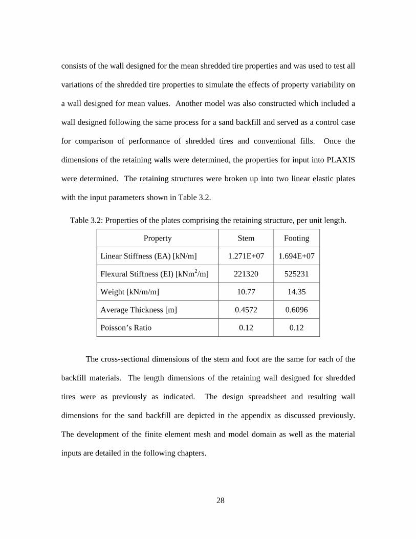
Table 3.2: Properties of the plates comprising the retaining structure, per unit length.
Property Stem Footing
Linear Stiffness (EA) [kN/m] 1.271E+07 1.694E+07
Flexural Stiffness (EI) [kNm2/m] 221320 525231
Weight [kN/m/m] 10.77 14.35
Average Thickness [m] 0.4572 0.6096
Poisson’s Ratio 0.12 0.12
The cross-sectional dimensions of the stem and foot are the same for each of the
backfill materials. The length dimensions of the retaining wall designed for shredded
tires were as previously as indicated. The design spreadsheet and resulting wall
dimensions for the sand backfill are depicted in the appendix as discussed previously.
The development of the finite element mesh and model domain as well as the material
inputs are detailed in the following chapters.

29
CHAPTER 4
FINITE ELEMENT MODELING METHODS
For this study, all modeling of the retaining structure and soil was performed
using the 2-D finite element software PLAXIS. This allows for the application of static
and dynamic loads and the analysis of both soil and wall responses. The model generally
consists of a gravity-cantilever retaining wall backfilled with shredded tires or sand. The
soils and shredded tire backfill were modeled using either the Mohr-Coulomb material
model or Hardening Soil model in PLAXIS as discussed further in following sections
while the structure was modeled using linear elastic plates.
For all of the study models, Standard Fixities and Standard Earthquake
Boundaries were applied. In PLAXIS, the Standard Fixities fix the sides of the model
against translation in the x-direction while fixing the base against translation in both the
x- and y-directions. The Standard Earthquake Boundaries include absorbent boundaries
on the vertical bounds of the soil body and apply a dynamic prescribed displacement to
the base of the model. The prescribed displacement is defined by the input of a
displacement, velocity, or acceleration time history, the latter two of which are converted,
using Newmark integration to a displacement time history. For all of the studies in this
research, the first 10 sec of the acceleration time history for the El Centro 1940
earthquake was applied to the base of the model using this prescribed displacement. El
Centro was used as the location for the wall design as well as is detailed in the previous
section. This acceleration time history is shown in Figure 4.1.
30
Figure 4.1: The portion of the El Centro 1940 acceleration time history applied.
First, the finite element model had to be further developed to achieve the
appropriate precision. The size and fineness of the model and finite element mesh were
determined through mesh sensitivity and size sensitivity analyses. For the most
representative results from the numerical model, it is important to first determine how
many elements need to be used to achieve appropriate sensitivity and precision in the
calculations. In this investigation, it was important to ensure that the results were not
dependent on the fineness of the finite element mesh.
Selection of Appropriate Finite Element Mesh
In order to select the appropriate mesh fineness for the study model, we first
created a sample model with a sample in-situ clay material, shredded tire backfill, and
retaining wall for which we could vary the fineness of the finite element mesh. Figure
4.2 shows the four meshes considered which include the Coarse (121 triangular elements
and 1059 nodes), Medium (262 elements and 2225 nodes), Fine (473 elements and 3967
nodes), and Very Fine (1061 elements and 8747 nodes) meshes in PLAXIS.
-4.0
-3.0
-2.0
-1.0
0.0
1.0
2.0
3.0
4.0
0 1 2 3 4 5 6 7 8 9 10
Acc
eler
atio
n (m
/s2 )
Time (sec)

31
(a) Coarse Mesh (121 triangular elements and 1059 nodes)
(b) Medium Mesh (262 elements and 2225 nodes)
(c) Fine Mesh (473 elements and 3967 nodes)

32
(d) Very Fine Mesh (1061 elements and 8747 nodes) Figure 4.2: Mesh fineness options observed in PLAXIS.
Because the movement of the wall tip was a major consideration in determining
the wall deflection, this was the first parameter to be observed. The deflection-time
history of the wall tip for each mesh was determined and the results of this test are shown
in Figure 4.3. The fineness of the mesh does not appear to greatly affect the displacement
of the wall tip. Additionally, in the model tests, the shear and moment behavior of the
wall were of interest so these were compared for each mesh. For consistency, the shear
and moment distributions on the wall stem were observed at the end of the dynamic
loading cycle for each of the meshes and these results are shown in Figure 4.4. Here the
mesh fineness caused little change in the wall response but the finer meshes do tend to
converge in both the shear and the bending moment distributions. Based on these results,
the Very Fine mesh, a term used in PLAXIS to denote highest level of mesh fineness,
was selected as the most appropriate mesh fineness for further studies.

33
Figure 4.3: Displacement time history for the retaining wall tip for each mesh fineness.
Figure 4.4: The shear and bending moment distributions in the retaining wall at the end of
dynamic loading for each mesh fineness.
0 2 4 6 8 10Dynamic Time [sec]
-0.1
0
0.1
0.2
0.3
0.4
Wal
l Tip
Dis
plac
emen
t [m
]
Very Fine MeshFine Mesh
Medium Mesh
Coarse Mesh
0 20 40 60Shear Force [kN/m]
0
1
2
3
4
5
6
7
Wal
l Hei
ght [
m]
Very Fine Mesh
Fine Mesh
Medium Mesh
Coarse Mesh
0 80 160Bending Moment [kNm/m]
0
1
2
3
4
5
6
7
Wal
l He
igh
t [m
]
Very Fine Mesh
Fine Mesh
Medium Mesh
Coarse Mesh

34
Selection of Appropriated Finite Element Domain
In addition to determining the necessary mesh fineness, it is important to
eliminate the effect of the location of boundaries as much as possible in order to get a
representative result. Although the boundary conditions recommended by the software
were used for the simulation, it is necessary to determine the size of the simulation
domain such that the computed responses are not affected by the selected boundary
condition. To do this, using the Very Fine mesh previously selected, the width of the
model was varied as shown in Figure 4.5.
Figure 4.5: Mesh showing variation lengths A and B for size sensitivity study.
Five cases were observed: Case 1 where A=7.62m (25’) and B=10.67m (35’),
Case 2 where A=9.14m (30’) and B=12.19m (40’), Case 3 where A=10.67m (35’) and
B=13.72m (45’), and Case 4 where A=12.19m (40’) and B=15.24m (50’). For each
model width the tip displacement time history and the shear and moment distribution in
the wall at the cessation of the dynamic loading were observed. The displacement time
history for the tip of the retaining wall is shown for all four cases in Figure 4.6.

35
Figure 4.6: Displacement time history for the retaining wall tip for each model size.
Based on these results it was clear that the model width affected the tip
displacement behavior but that as the model size increased, some convergence was
observed. The three largest sizes converged best but showed some variation between
Case 2 and Cases 3 and 4 early in the dynamic load and between Case 3 and Cases 2 and
4 later in the loading. Because a larger model will only serve to reduce misleading
effects of the boundary conditions, and because Case 4 most consistently converged with
other results throughout the test, it was considered most appropriate based on wall tip
displacement. Next the shear and moment distributions in the wall were observed
following the dynamic loading sequence for all of the cases. Shown in Figure 4.7, these
results again show how the size used in Case 4 allows for differences in the wall
behavior. Here the Case 4 model displayed a less restricted response in the shear and
bending moment of the wall. This decrease in boundary based restriction and the better
0 2 4 6 8 10Dynamic Time [sec]
-0.1
0
0.1
0.2
0.3
0.4
Wal
l Tip
Dis
plac
emen
t [m
]
Case 1Case 2
Case 3
Case 4

36
convergence in the wall tip displacement indicated that Case 4 was a suitable model
geometry for future study.
Figure 4.7: The shear and bending moment distributions in the retaining wall at the end of
dynamic loading for each model size.
Final Finite Element Model
Based on this mesh sensitivity and size sensitivity study, the mesh fineness and
model size were determined. This, combined with the selected boundary conditions and
retaining wall design dimensions, was used to create the basic finite element model that
would be used for all studies. This configuration is depicted for shredded tire backfill in
Figure 4.8. For conventional sand fills, the wall and backfill zone dimensions were
adjusted but the model domain and mesh fineness remained the same.
0 20 40 60Shear Force [kN/m]
0
1
2
3
4
5
6
7W
all H
eigh
t [m
]Case 1
Case 2
Case 3
Case 4
-200 -100 0 100 200Bending Moment [kNm/m]
0
1
2
3
4
5
6
7
Wal
l He
igh
t [m
]
Case 1
Case 2
Case 3
Case 4

37
Figure 4.8: Finite element mesh used in all studies.
As shown in the final model configuration, the model generally consists of the
retaining wall, backfill material, and some in-situ material. The wall is as designed in the
previous section and the material properties assigned to the plates are as previously
described . The backfill material and in-situ material properties are defined based on the
material model and property variation being considered for each of the studies in this
research. All of the soil material input parameters used in this model are detailed in later
chapters.
38
CHAPTER 5
DAMPING AND MATERIAL MODELING
In general dynamic behavior, the equation of motion shown below is used to
describe the system behavior in terms of its mass, stiffness, and damping characteristics
as well as the forcing function.
��� + ��� + �� = �� (1)
In this equation, M is the mass matrix, C is the viscous damping matrix, and K is
the stiffness matrix and F(t) represents the forcing function if applicable. These
characteristics are based on the physical properties and boundary conditions of the system
and can describe the vibration and dynamic response of the system.
When the material being considered is a soil, the stiffness matrix and damping
matrix are not necessarily constant with shear strain, neither spatially nor throughout the
loading application time. Both damping and shear modulus vary with the strain induced
in the soil at the different locations in the model. Thus, in the dynamic modeling of soils,
two main considerations primarily govern the precision with which the model describes
the behavior of the system: damping and modulus reduction with shear strain. Damping
includes viscous damping, that due to movement of the pore fluid and particle friction,
and hysteretic damping, that due to energy lost during plastic deformation in cyclic
loading. The modulus reduction refers to the loss of soil stiffness with increasing strain
induced in the soil which is indicated by a reduction in the shear modulus of the soil at a
higher strains. This is typically depicted by a non-linear stress-strain curve such as the
hyperbolic Hardening Soil Model described later. Different material models can be

39
compared primarily by how each describes this behavior and fits the realistic curve for
the material.
For this study, the problem statement and reliability study scenarios were modeled
considering three different combinations of damping and material model. The primary
results were obtained using the Hardening Soil Model, the most advanced of the material
models considered, and Rayleigh damping. In addition, parametric studies were
performed utilizing the Mohr-Coulomb Model with Rayleigh damping and using the
Mohr-Coulomb model with no external damping applied. The combinations of damping
and material model were selected based on their varying abilities to handle modulus
reduction and damping as well as the availability of material information. Damping and
material behavior based on the combinations of the material models and external
damping are described in detail below.
Rayleigh Damping
In order to model the damping in the system due to fluid motion and friction
(viscous damping), an external damping in the form of Rayleigh damping is implemented
in PLAXIS. This Rayleigh damping is used in most of the site response analysis tools
such as D-MOD, DeepSoil and OpenSees. The stiffness and mass proportional (full)
Rayleigh damping formulation is shown in equation 2.
�� = ��� + ��� (2)
where M is the mass matrix, K is the stiffness matrix, and CR is the Rayleigh
damping matrix. The input of these parameters (α and β) allows for the formulation of the
external damping matrix for the soils regardless of the material model and resulting

40
material damping being considered. The formulation of these parameters is given by the
following equations:
�� = ����� � �
���� (3)
�� = ���� � �
���� (4)
where T is the predominant period of the soil body, is the target damping and n
is an odd integer related to the mode numbers at which the target damping is matched.
The odd integer n is a constant that corresponds to the mode by the following equation:
� = 2� − 1 (5)
where m is the mode being considered. For geotechnical problems, the third
mode is often used because much of the dynamic energy is condensed to the third mode
and it is a commonly used measuring point for dynamic properties. This indicated a
mode number (n) of 5 for the study being conducted. Also the target damping had to be
selected. As this value cannot be determined with certainty without direct testing of the
system, a reasonable and commonly used value of 5% was used for the target damping
(Phillip and Hashash, 2009).
Based on soil properties it is possible to determine the predominant period of the
soil body by the following equation.
� =��
�,��� (6)
where H is the thickness of the soil layer and Vs,ave is the average soil shear wave
velocity. The shear wave velocity of the soils and shredded tires in this case were

41
calculated in PLAXIS based on modulus and Poisson’s Ratio inputs corresponding to the
material definition.
Based on these parameters, the Rayleigh Damping values were determined for
each material (in-situ clay and shredded tires). These values can be directly input into
PLAXIS to apply an external viscous damping to the system. The equation of motion for
the system with the external damping can then be described as
��� + ���� + �� = �() (7)
where u is the nodal displacement, F(t) is the forcing function, and all other
variables are as previously defined.
The Mohr-Coulomb Material Model
The simpler of the two material models applied was the Mohr-Coulomb model.
This model is a two-part model consisting of an elastic portion and a perfectly plastic
portion. In PLAXIS, the elastic portion is described by the input of the Young’s Modulus
at reference confining pressure and Poisson’s ratio for the soil while the plastic portion is
governed by the Mohr-Coulomb criteria of the friction angle (φ) and cohesion (c). The
stress-strain model used in PLAXIS is depicted in Figure 5.1. This model is familiarly
used in geotechnical engineering practice and provides an over-simplified description of
soil behavior but uses commonly available input parameters for soils.

42
Figure 5.1: Mohr-Coulomb Stress-Strain Criterion based on PLAXIS input parameters
Due to the elastic-perfectly plastic model, this material model has some
limitations; however, this model was attractive because the properties of shredded tires
and soils that were readily available were compatible with this commonly used model.
Because of this, the advantage of this model lies in the wide range of lab tests available to
provide input parameter values. Specific experimental values for all Mohr-Coulomb
input parameters were able to be obtained from the literature and statistical analysis could
be performed for the range of values provided. The more advanced Hardening Soil
model described in the following subsection requires multiple modulus values that are not
commonly tested for in practical applications and require calibration if the soil or
shredded tires are going to be modeled accurately. This fact added validity to the use of
the Mohr-Coulomb material model.

43
The primary limitations to this model were lack of ability to model modulus
reduction and hysteretic damping during cyclic loading. The Mohr-Coulomb material
model models all behavior with stresses below the plastic point as a linear elastic
material. This means that as loading and unloading is applied, the soil is elastic up until
the plastic point, where it begins to exhibit perfectly plastic behavior, and when
unloading begins, it returns along a linear elastic path parallel to the original loading
curve. This means two things: elastic-perfectly plastic modeling does not account for
modulus reduction with increasing shear strain and hysteresis behavior typical for soil
and other geotechnical engineering materials. Because of this, the main strength of the
model was the accuracy of the inputs based on multiple different lab test results on a wide
range of materials, and external viscous damping was applied in the second case
considered to help give more realistic dynamic characteristics to the model in the absence
of hysteretic damping in the material model.
The Hardening Soil Model
The more advanced material model applied was the Hardening Soil model. This
model is an advanced multi-part hyperbolic model that improves upon conventional
elastic-perfectly plastic models and simpler hyperbolic models by including parameters to
encompass the modulus reduction of soil and include better approximations of plastic
strain and dilatancy. The main components of this model are stress dependent stiffness,
plastic strain due to multiple types of loading, unloading and reloading characteristics,
and Mohr-Coulomb failure criterion. These criteria are shown in Figure 5.2 which
depicts the stress-strain curve for the Hardening Soil Model in PLAXIS.

44
Figure 5.2: Hardening Soil Model Stress-Strain Criteria based on PLAXIS input
parameters
First this model allows for exponential stiffness changes with applied stress and
strain using the input of the fitting parameter “m.” The “m” parameter dictates how
much influence the applied stress has over the modulus. This coupled with the input of
the modulus of elasticity at 50% of the yield stress at reference pressure (E50,ref) creates a
hyperbolic shear stress-strain curve that depicts a continuous modulus reduction for each
strain value. Other modulus inputs dictate loading and unloading behavior and the secant
modulus to further complete the hyperbolic curve. This curve, in conjunction with the
Mohr-Coulomb parameters dictating the failure envelope, allow for a much more precise
characterization of the soil behavior particularly through loading and unloading cycles
imposed by seismic loading. The use of these modulus values fills in the problems with
the Mohr Coulomb model by acknowledging that the behavior below the plastic failure

45
point is not linear elastic and thus providing a more accurate representation of soil
behavior in that range. In addition, this and the use of specific loading and unloading
modulus values more accurately represent the stress-strain characteristics of the soil
under cyclic loads.
The only hurdle with the use of the Hardening-Soil model to model the shredded
tires was a lack of detailed modulus information. This required a combination of
calibration procedures that used Mohr-Coulomb data that was known from the literature
and a select few sets of experimental results which depicted the hyperbolic behavior of
the shredded tires and from which some modulus information could be inferred. Based
on some modulus information, the established Mohr-Coulomb failure criterion, and curve
fitting between the Hardening Soil Model and experimental data and the Mohr-Coulomb
model, reasonable input values were selected. The selection of some input parameters
were also based on default relationships recommended for the proper function of
PLAXIS. A detailed account of the calibration procedures and resulting inputs follows.
In terms of damping, though this model can encompass loading and unloading
modulus characteristics, it does not incorporate hysteretic damping. That being said, it
was still necessary to apply the external Rayleigh Damping to these models to attempt to
get a realistic response. The Rayleigh Damping parameters were computed as previously
described. In order to even more accurately model the damping characteristics of
shredded tires, however, it is necessary to use an appropriate material model that includes
hysteresis in the formulation as well as viscous damping provisions.

46
CHAPTER 6
DETERMINATION OF MODEL INPUT PARAMETERS
As discussed in the previous chapter, modeling accuracy and robustness varies
based on how much is known about the material in terms of available input parameters as
well as the ability of the modeling technique to capture all behavioral aspects. For this
research many variations in the input parameters were considered to observe the effects
of variation in the material properties through parametric study as well as to identify the
most robust and effective way to model the system with different material models and
damping schemes. This meant that the study was broken down into components
including three parametric studies, one using the Mohr-Coulomb material model and no
damping, one using the Mohr-Coulomb model and Rayleigh damping, and one using the
Hardening-Soil model an Rayleigh damping; a comparison of systems with and without
Rayleigh damping; and a comparison of using the Mohr-Coulomb material model and the
Hardening-Soil material model. In the following sections, the methods for determining
the material input parameters for all models are described in the order in which they were
implemented and the resulting values are provided in summary.
Determination of the Mohr-Coulomb Parameters
The input parameters for all models using the Mohr-Coulomb material model
were gained from the literature. The studies from which these properties were obtained
consisted of many types of tests on many different types and sizes of shredded tires. This
included primarily lab tests, either standard geotechnical tests or modified tests. The full
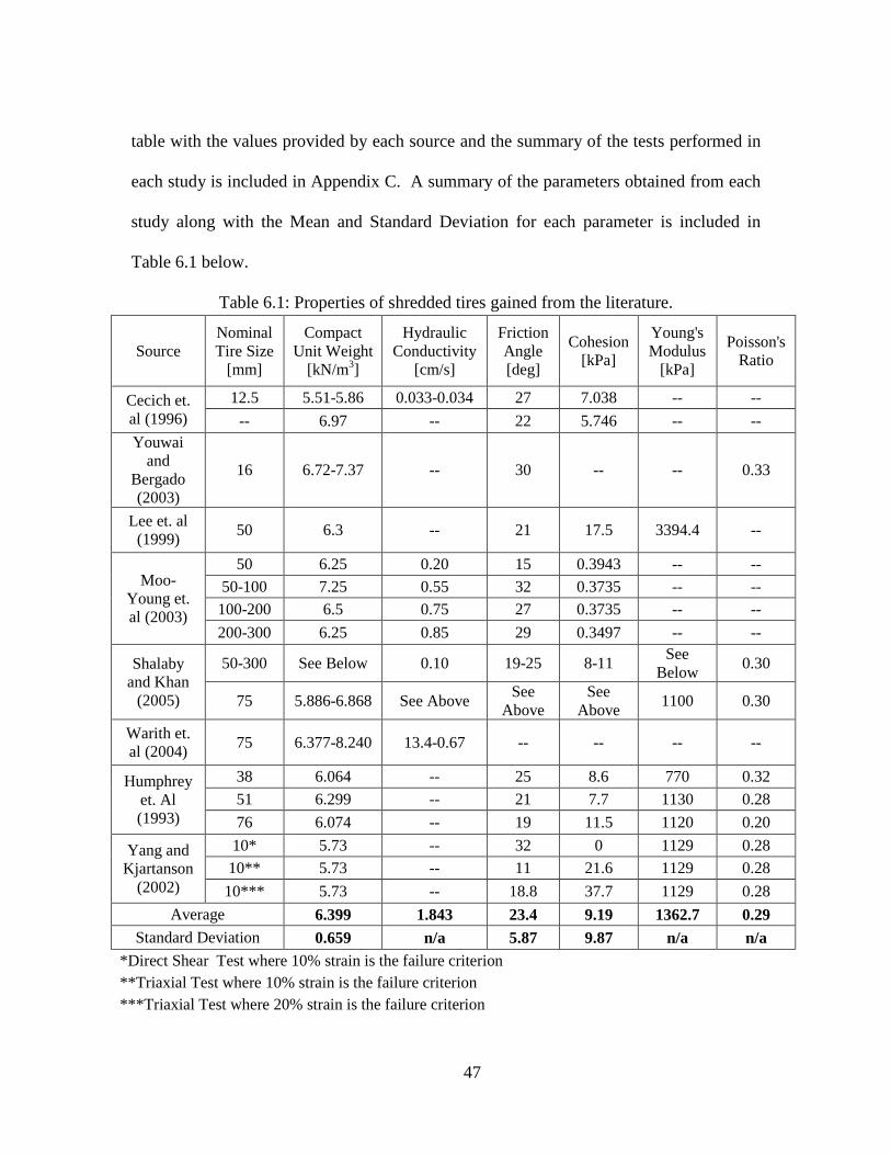
47
table with the values provided by each source and the summary of the tests performed in
each study is included in Appendix C. A summary of the parameters obtained from each
study along with the Mean and Standard Deviation for each parameter is included in
Table 6.1 below.
Table 6.1: Properties of shredded tires gained from the literature.
Source Nominal Tire Size
[mm]
Compact Unit Weight
[kN/m3]
Hydraulic Conductivity
[cm/s]
Friction Angle [deg]
Cohesion [kPa]
Young's Modulus
[kPa]
Poisson's Ratio
Cecich et. al (1996)
12.5 5.51-5.86 0.033-0.034 27 7.038 -- --
-- 6.97 -- 22 5.746 -- -- Youwai
and Bergado (2003)
16 6.72-7.37 -- 30 -- -- 0.33
Lee et. al (1999)
50 6.3 -- 21 17.5 3394.4 --
Moo-Young et. al (2003)
50 6.25 0.20 15 0.3943 -- --
50-100 7.25 0.55 32 0.3735 -- --
100-200 6.5 0.75 27 0.3735 -- --
200-300 6.25 0.85 29 0.3497 -- --
Shalaby and Khan
(2005)
50-300 See Below 0.10 19-25 8-11 See
Below 0.30
75 5.886-6.868 See Above See
Above See
Above 1100 0.30
Warith et. al (2004)
75 6.377-8.240 13.4-0.67 -- -- -- --
Humphrey et. Al (1993)
38 6.064 -- 25 8.6 770 0.32
51 6.299 -- 21 7.7 1130 0.28
76 6.074 -- 19 11.5 1120 0.20
Yang and Kjartanson
(2002)
10* 5.73 -- 32 0 1129 0.28
10** 5.73 -- 11 21.6 1129 0.28
10*** 5.73 -- 18.8 37.7 1129 0.28
Average 6.399 1.843 23.4 9.19 1362.7 0.29 Standard Deviation 0.659 n/a 5.87 9.87 n/a n/a
*Direct Shear Test where 10% strain is the failure criterion **Triaxial Test where 10% strain is the failure criterion ***Triaxial Test where 20% strain is the failure criterion

48
These mean and standard deviation values were used to construct variations in
material properties that were used for the parametric study and were used to determine
the statistical relationships considered in the subsequent reliability analysis. The friction
angle, cohesion, and unit weight of the shredded tire fill were the parameters of interest in
this study and the ones for which the most statistical information was available. Each of
these material properties were varied with respect to the mean value by one, two, and
three standard deviations above and below, and the resulting variations are summarized at
the end of this chapter. Once all the variation had been determined, they could be used
both in the PLAXIS model and then be extrapolated to the calibration of the hardening
soil parameters. The process for determining the Hardening Soil model parameters based
on the Mohr-Coulomb properties is described in the following section.
Calibration of the Hardening Soil Model
As previously described, the Hardening Soil Model, while giving a better
representation of shredded tire material behavior, requires a number of specific
parameters to do so and these parameters have not been experimentally determined in
past studies. This required graphical calibration of Hardening Soil parameters to
experimental data and Mohr-Coulomb parameters if input values were to be determined
for the PLAXIS inputs. The first step in this process involved identifying all necessary
input parameters and what they mean as well as how they are connected in explaining the
soil behavior. Table 6.2 shows a list of the parameters required by the Hardening Soil
model in PLAXIS with what each represents. Many of these parameters are represented
graphically in the previous section.

49
Table 6.2: Parameter Definitions for the Hardening Soil Model in PLAXIS
Behavior Below Failure Envelope
��� � Secant modulus at 50% of the failure stress at the Reference Confining Pressure
�� �� � Initial tangent modulus for the oedometer loading
���� � Unloading and Reloading modulus at Reference Confining Pressure
� Power dictating the stress-modulus dependency
Failure Parameters
� Mohr- Coulomb Cohesion
� Mohr-Coulomb Friction Angle
Each of these calibration parameters is used in conjunction with formulas in
PLAXIS that define the asymptote, failure line, and curvature of the graph of the material
behavior. By applying the formulas used by PLAXIS in a spreadsheet, it was easy to
compare graphically the curve created for the Hardening Soil model with experimental
data and eventually the Mohr-Coulomb curves for the known cases being modeled.
During calibration it was first important to note what each parameter dictates in
the construction of the curve and the resulting representation of soil behavior both at the
reference pressure and at other confining pressures. First, the Mohr-Coulomb parameters
define the failure criterion based on the friction angle and cohesion according to the
following equation.
�� = (� cot�� − ���) ����(�)
�������� (8)

50
where σ3’ is the confining pressure being observed, and qf is the failure deviator
stress. Once the Hardening Soil curve intersects this envelope, it assumes perfectly
plastic behavior. This equation also shows how the magnitude of the failure stress varies
with the confining stress. In addition to a defined failure envelope, the Hardening Soil
model uses an asymptote as discussed in the previous sections. The asymptotic deviator
stress is defined in terms of the failure deviator stress as follows where Rf has a default
value of 0.9.
�� =��
�� (9)
In all cases, these equations reflect sign conventions where compression is
negative for confining stresses. These equations dictate the “height” of the curve as it
approaches the failure stress as well as the strain at which the material becomes perfectly
plastic. It is important to note that these characteristics are determined based on the
friction angle and cohesion which are known values for shredded tires based on lab test
data and are the same as those used in simulations using the Mohr-Coulomb material
model. These values were thus considered “fixed” in the calibration process.
In dictating the shape of the initial loading curve, the ��changes the steepness of
the initial curvature of the curve by indicating the slope at 50% of the failure deviator
stress. The value of this parameter is provided at the reference pressure but it is related
at varying confining stress by the following equation.
�� = ��� � ��∗ !�����"�
� ������
� !�����#��� �������$
(10)

51
This equation also shows how the m parameter dictates the dependency of the
modulus on the confining stress. Thus, the effects of m are seen in calibrations at other
confining pressures and it is noted that it primarily changes the curvature of the initial
loading curve with higher values of m increasing curvature for the same ��� � .
Once these parameters for the initial loading curve are determined, the
corresponding strain values are determined based on the following relationship.
� =�
%∗
�
��
�
(11)
�ℎ���:�& =2��
2 − ��
This allowed for the plotting of the initial loading curve and the resulting
calibration, achieved by changing the ��� � and the m values as described in detail in the
following sections.
In order to define the parameters for the loading-unloading behavior, no
information was known to compare to and calibrate to so some correlations
recommended by PLAXIS were utilized. First, the �� �� � given by PLAXIS for the known
Young’s Modulus and Mohr Coulomb Criterion was used. Second, the ���� � was taken
as 3��� �as recommended for use in PLAXIS.
Calibration to Available Experimental Data
The first step in the calibration process was to calibrate the Hardening Soil Model
to the experimental data and to observe the resulting graphical correlation between the
Hardening Soil Model and the Mohr Coulomb Model to be used to calibrate cases where

52
only Mohr-Coulomb data was available. The correlation between the Mohr Coulomb and
Hardening Soil models that resulted would be used as a basis for calibration of the
Hardening Soil Parameters to meet the Mohr Coulomb behavior in the cases being
considered in the simulations.
In calibrating to the experimental data, the first step was to determine the Mohr
Coulomb failure criterion that is indicated by the experimental data. The failure deviator
stress was determined based on that which produced a 25% strain. This seemed
reasonable both based on the nature of the problem and the observed experimental
behavior that plateaus at approximately that point in general. The resulting friction angle
and cohesion values were used in the graphing of both the Mohr Coulomb and Hardening
Soil Models. From there it was necessary to calibrate the two other parameters for the
Hardening Soil Model: the ��� �and m.
For the determination of the ��� �value, the graph experimental data from Youwai
and Bergado (2003) was used as shown in Figure 6.1(a). Because this data was collected
at reference confining pressure, the modulus at 50% of the failure deviator stress
indicated the ��� � value for shredded tires and could be calculated directly. Using this
value and the friction angle and cohesion values computed based on the failure deviator
stress were used to plot the Mohr-Coulomb and Hardening Soil models alongside the
experimental data.

53
(a) Youwai and Bergado (2003) (b) Youwai and Bergado (2003)
(c) Yang and Kjartanson (2002) (d) Yang and Kjartanson (2002)
Figure 6.1: Graphical calibration of Hardening Soil Model to experimental data and Mohr Coulomb criterion from two sources and four confining pressures.
Once this value had been determined for experimental calibrations, it was
necessary to calibrate the m value, which is only observed at confining pressures other
than the reference pressure. For this, the ��� �parameter was kept constant and

54
experimental data from Youwai and Bergado (2003) and Yang and Kjartanson (2002) at
varying confining pressures were plotted. The Mohr-Coulomb and Hardening Soil
models were plotted as before based on the calculated friction angle and cohesion for
each data set and the ��� �value determined at the reference pressure. Then the m value
was adjusted to fit most approximately the experimental data with the Hardening Soil
model. This process and the resulting Mohr-Coulomb and Hardening Soil graphical
relationships are shown in Figure 6.1(b)-(d).
The quality of fit between the Hardening Soil model and the Mohr-Coulomb
model and experimental data was somewhat limited by the restraints of the friction angle
and cohesion which define the asymptote for the Hardening Soil model. It should also be
noted that the flexibility of the Hardening Soil model is limited by its formulation. Except
the parameter m, all the other variables in the Hardening Soil model need to be
determined from experimental data. Also, this model was developed to represent the
shear stress-strain behavior of soil, which is different from shredded tire. Because of the
low initial modulus of the shredded tires, the amount of adjustment to the fit from ��� � is
limited and thus, the modulus computed by the Hardening Soil model is less than that of
the Mohr-Coulomb and even the experimental data. For the variations in shredded tire
material properties previously considered, Mohr-Coulomb parameters were available, and
thus, the graph of the Mohr-Coulomb behavior was the point of comparison for
calibrating the Hardening Soil Model parameters. Because of this, the fit observed
between the Mohr-Coulomb model and the Hardening Soil model that best fit the
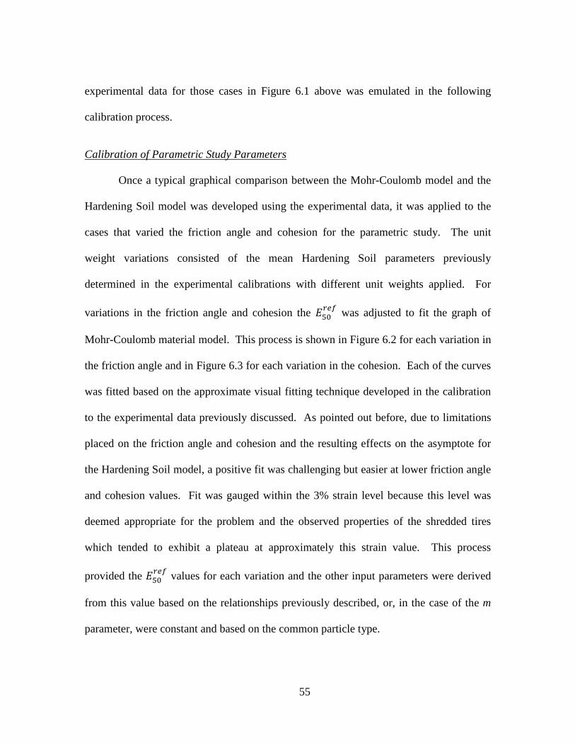
55
experimental data for those cases in Figure 6.1 above was emulated in the following
calibration process.
Calibration of Parametric Study Parameters
Once a typical graphical comparison between the Mohr-Coulomb model and the
Hardening Soil model was developed using the experimental data, it was applied to the
cases that varied the friction angle and cohesion for the parametric study. The unit
weight variations consisted of the mean Hardening Soil parameters previously
determined in the experimental calibrations with different unit weights applied. For
variations in the friction angle and cohesion the ��� � was adjusted to fit the graph of
Mohr-Coulomb material model. This process is shown in Figure 6.2 for each variation in
the friction angle and in Figure 6.3 for each variation in the cohesion. Each of the curves
was fitted based on the approximate visual fitting technique developed in the calibration
to the experimental data previously discussed. As pointed out before, due to limitations
placed on the friction angle and cohesion and the resulting effects on the asymptote for
the Hardening Soil model, a positive fit was challenging but easier at lower friction angle
and cohesion values. Fit was gauged within the 3% strain level because this level was
deemed appropriate for the problem and the observed properties of the shredded tires
which tended to exhibit a plateau at approximately this strain value. This process
provided the ��� � values for each variation and the other input parameters were derived
from this value based on the relationships previously described, or, in the case of the m
parameter, were constant and based on the common particle type.

56
0 0.1 0.2 0.3Strain
0
80
160
240
320
400
480D
evi
ator
Str
ess
(kP
a)
Mohr Coulomb
Hardening Soil
Mean + 3σ
0 0.1 0.2 0.3
Strain
0
80
160
240
320
400
Devi
ator
Str
ess
(kP
a)
Mohr Coulomb
Hardening Soil
Mean + 2σ
0 0.1 0.2 0.3Strain
0
40
80
120
160
200
240
Dev
iato
r S
tres
s (k
Pa)
Mohr CoulombHardening Soil
Mean + 1σ
0 0.1 0.2 0.3Strain
0
20
40
60
80
Dev
iato
r S
tres
s (k
Pa)
Mohr Coulomb
Hardening Soil
Mean - 2σ
Figure 6.2: Calibration of Hardening Soil Model for the variations in the Friction Angle.
0 0.1 0.2 0.3Strain
0
20
40
60
Dev
iato
r S
tres
s (k
Pa)
Mohr Coulomb
Hardening Soil
Mean - 3σ

57
0 0.1 0.2 0.3Strain
0
40
80
120
160
200
240
280D
evia
tor
Stre
ss (
kPa)
Mohr Coulomb
Hardening Soil
Mean + 3σ
0 0.1 0.2 0.3
Strain
0
40
80
120
160
200
240
Dev
iato
r S
tres
s (k
Pa)
Mohr Coulomb
Hardening Soil
Mean + 2σ
0 0.1 0.2 0.3Strain
0
40
80
120
160
200
Dev
iato
r St
ress
(kP
a)
Mohr Coulomb
Hardening Soil
Mean + 1σ
0 0.1 0.2 0.3
Strain
0
40
80
120
160D
evia
tor
Stre
ss (
kPa)
Mohr Coulomb
Hardening Soil
Mean - 1σ
Figure 6.3: Calibration of Hardening Soil Model for the variations in the Cohesion.
Material Properties and Input Parameters
This process combined with the default values and correlations in PLAXIS
previously discussed allow for the determination of all the input parameters for variations
utilizing the Hardening Soil model. Once the hardening soil parameters had been
generated, this completed the set of input parameters for all of the studies to be
performed.
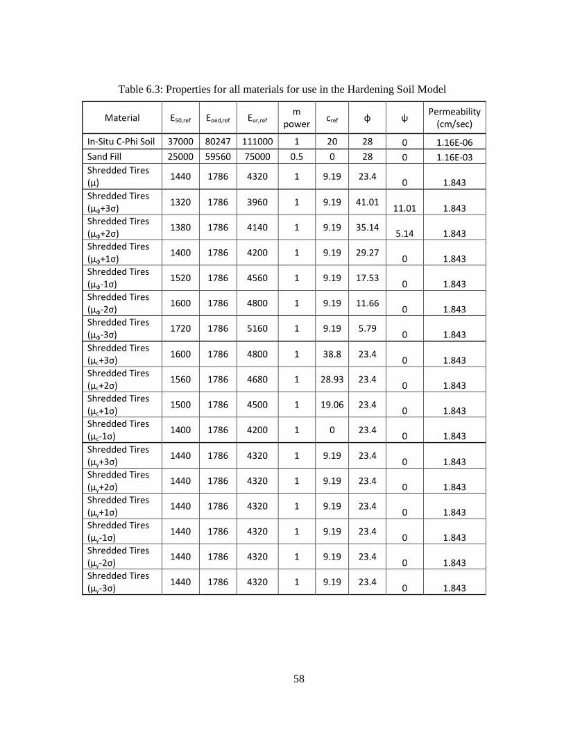
58
Table 6.3: Properties for all materials for use in the Hardening Soil Model
Material E50,ref Eoed,ref Eur,ref m
power cref φ ψ
Permeability
(cm/sec)
In-Situ C-Phi Soil 37000 80247 111000 1 20 28 0 1.16E-06
Sand Fill 25000 59560 75000 0.5 0 28 0 1.16E-03
Shredded Tires
(µ) 1440 1786 4320 1 9.19 23.4
0 1.843
Shredded Tires
(µφ+3σ) 1320 1786 3960 1 9.19 41.01
11.01 1.843
Shredded Tires
(µφ+2σ) 1380 1786 4140 1 9.19 35.14
5.14 1.843
Shredded Tires
(µφ+1σ) 1400 1786 4200 1 9.19 29.27
0 1.843
Shredded Tires
(µφ-1σ) 1520 1786 4560 1 9.19 17.53
0 1.843
Shredded Tires
(µφ-2σ) 1600 1786 4800 1 9.19 11.66
0 1.843
Shredded Tires
(µφ-3σ) 1720 1786 5160 1 9.19 5.79
0 1.843
Shredded Tires
(µc+3σ) 1600 1786 4800 1 38.8 23.4
0 1.843
Shredded Tires
(µc+2σ) 1560 1786 4680 1 28.93 23.4
0 1.843
Shredded Tires
(µc+1σ) 1500 1786 4500 1 19.06 23.4
0 1.843
Shredded Tires
(µc-1σ) 1400 1786 4200 1 0 23.4
0 1.843
Shredded Tires
(µγ+3σ) 1440 1786 4320 1 9.19 23.4
0 1.843
Shredded Tires
(µγ+2σ) 1440 1786 4320 1 9.19 23.4
0 1.843
Shredded Tires
(µγ+1σ) 1440 1786 4320 1 9.19 23.4
0 1.843
Shredded Tires
(µγ-1σ) 1440 1786 4320 1 9.19 23.4
0 1.843
Shredded Tires
(µγ-2σ) 1440 1786 4320 1 9.19 23.4
0 1.843
Shredded Tires
(µγ-3σ) 1440 1786 4320 1 9.19 23.4
0 1.843
59
Table 6.3 shows the input parameters for all soils and shredded tire material
variations for use in the Hardening soil model. The Mohr-Coulomb parameters that were
used for calibrating the Hardening Soil model parameters as well as in simulations that
utilized the Mohr-Coulomb material model are shown in Table 6.4 below. These
material properties were combined with properties of the linear elastic plates that make
up the retaining structure as well as the finite element mesh and domain developed (both
discussed previously) to complete the set of finite element models used in the studies.
Table 6.4: Properties for all materials for use in the Mohr-Coulomb Model
Material
Young's
Modulus
(kPa)
Poisson's
Ratio
Permeability
(cm/sec)
Unit
Weight
(kN/m3)
Cohesion
(kPa)
Friction
Angle
(deg)
In-Situ C-Phi Soil 50000 0.35 1.16E-06 18.07 20 28
In-Situ Clay 85992.5 0.35 1.16E-06 18.07 110.67 0
Shredded Tires (µ) 1362.7 0.29 1.843 6.399 9.19 23.4
Shredded Tires (µφ+3σ) 1362.7 0.29 1.843 6.399 9.19 41.01
Shredded Tires (µφ+2σ) 1362.7 0.29 1.843 6.399 9.19 35.14
Shredded Tires (µφ+1σ) 1362.7 0.29 1.843 6.399 9.19 29.27
Shredded Tires (µφ-1σ) 1362.7 0.29 1.843 6.399 9.19 17.53
Shredded Tires (µφ-2σ) 1362.7 0.29 1.843 6.399 9.19 11.66
Shredded Tires (µφ-3σ) 1362.7 0.29 1.843 6.399 9.19 5.79
Shredded Tires (µc+3σ) 1362.7 0.29 1.843 6.399 38.8 23.4
Shredded Tires (µc+2σ) 1362.7 0.29 1.843 6.399 28.93 23.4
Shredded Tires (µc+1σ) 1362.7 0.29 1.843 6.399 19.06 23.4
Shredded Tires (µc-1σ) 1362.7 0.29 1.843 6.399 0 23.4
Shredded Tires (µγ+3σ) 1362.7 0.29 1.843 8.376 9.19 23.4
Shredded Tires (µγ+2σ) 1362.7 0.29 1.843 7.717 9.19 23.4
Shredded Tires (µγ+1σ) 1362.7 0.29 1.843 7.058 9.19 23.4
Shredded Tires (µγ-1σ) 1362.7 0.29 1.843 5.74 9.19 23.4
Shredded Tires (µγ-2σ) 1362.7 0.29 1.843 5.081 9.19 23.4
Shredded Tires (µγ-3σ) 1362.7 0.29 1.843 4.422 9.19 23.4

60
In addition to defining the material properties for each soil, some cases included
an applied viscous Rayleigh damping as previously described. These parameters were
developed according to the previously described equations to get the coefficients
displayed in Table 6.5. These coefficients were used in all cases where damping was
considered regardless of material model and are independent inputs from the model-
based inputs in PLAXIS.
Table 6.5: Rayleigh Damping Coefficients for Soils.
Soil Thickness (H) [m]
Shear Wave Velocity (Vs) [m/s]
Period (T) [sec]
αR
βR
Shredded Tires 9.6 28.44 0.8579 0.6103 0.002276
In-Situ Soils 6.1 131.40 0.292 1.793 0.000775
Sand Backfill 6.1 97.85 0.249 2.103 0.00066

61
CHAPTER 7
RESULTS AND DISCUSSION
The studies as discussed previously are broken up in three main cases based on
the material model and damping scheme used: Mohr-Coulomb (M-C) material model
without damping, Mohr-Coulomb material model with Rayleigh damping, and the
Hardening Soil material model with Rayleigh damping. This section highlights the
results from the most in depth model: the Hardening Soil material model with Rayleigh
damping. This included a comparison of wall performance with shredded tire backfill
and sand backfill as well as a parametric study utilizing the previously described
calibrated input parameters for shredded tire fill and a subsequent comparison of
maximum wall deflection, shear force, and bending moment for the wall.
Comparison with Standard Backfill
As discussed in the design section of this study, walls designed for use with
shredded tire fills provide an initial cost cutting benefit in terms of wall and backfill
materials as well as excavation and construction costs. These initial benefits make
shredded tire fill appear to be a good alternative to sand fills. In this portion of the study,
the two retaining walls with two different backfill materials were modeled and the
performance of the retaining wall in terms of wall deflections, shear forces, and bending
moments was observed based on conventional vs. alternative fills. The first performance
characteristic of interest was the deflection time history of the retaining wall. This is
depicted for both shredded tires and sand backfill in Figure 7.1.

62
Figure 7.1: Wall Deflection Time Histories for Sand and Shredded Tire Backfills
This graph represents the relative displacement of the wall tip to the base of the
stem throughout the dynamic loading application. It is apparent from this graph that the
shredded tires produced a lower deflection in the wall stem than the conventional sand
backfill in terms of deflection amplitude and total maximum deflection experienced
during the loading progression. The wall backfilled with conventional sand also
sustained more permanent wall deflection at the end of the dynamic loading indicating
that shredded tires may also offer benefits of resiliency. This is likely due to both the
lower deflections produced overall and the lower modulus but comparable limit strength
of the two fill materials.
Though these walls were designed for the retention of the fill they were modeled
with, the wall backfilled with the shredded tires still showed better deflection control than
0 2 4 6 8 10Dynamic Time (sec)
-2
-1
0
1
2
3W
all D
efle
ctio
n (c
m)
Conventional Sand
Shredded Tires
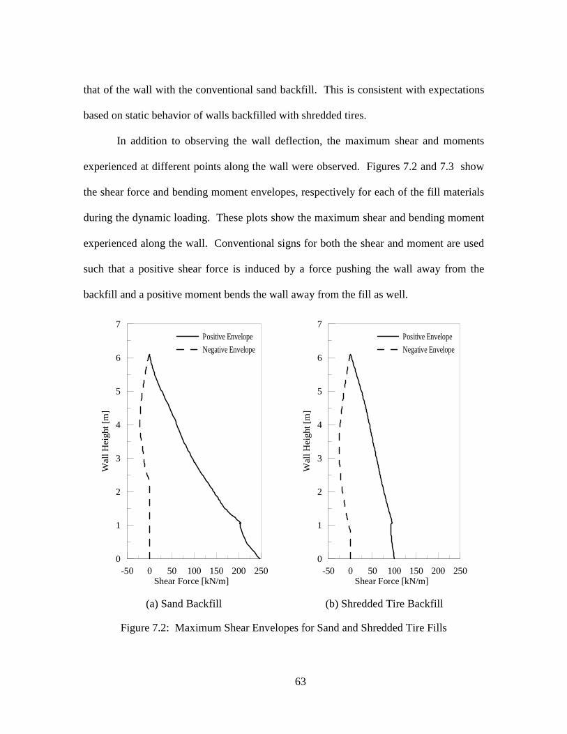
63
that of the wall with the conventional sand backfill. This is consistent with expectations
based on static behavior of walls backfilled with shredded tires.
In addition to observing the wall deflection, the maximum shear and moments
experienced at different points along the wall were observed. Figures 7.2 and 7.3 show
the shear force and bending moment envelopes, respectively for each of the fill materials
during the dynamic loading. These plots show the maximum shear and bending moment
experienced along the wall. Conventional signs for both the shear and moment are used
such that a positive shear force is induced by a force pushing the wall away from the
backfill and a positive moment bends the wall away from the fill as well.
-50 0 50 100 150 200 250Shear Force [kN/m]
0
1
2
3
4
5
6
7
Wal
l Hei
ght [
m]
Positive Envelope
Negative Envelope
-50 0 50 100 150 200 250
Shear Force [kN/m]
0
1
2
3
4
5
6
7
Wal
l Hei
ght [
m]
Positive Envelope
Negative Envelope
(a) Sand Backfill (b) Shredded Tire Backfill
Figure 7.2: Maximum Shear Envelopes for Sand and Shredded Tire Fills

64
-100 0 100 200 300 400 500 600Bending Moment [kNm/m]
0
1
2
3
4
5
6
7
Wal
l Hei
ght [
m]
Positive Envelope
Negative Envelope
-100 0 100 200 300 400 500 600
Bending Moment [kNm/m]
0
1
2
3
4
5
6
7
Wal
l Hei
ght [
m]
Positive Envelope
Negative Envelope
(a) Sand Backfill (b) Shredded Tire Backfill
Figure 7.3: Maximum Shear Envelopes for Sand and Shredded Tire Fills
At first glance, it is clear the shear force and bending moment induced in the wall
are less throughout the wall height when shredded tires are used in place of conventional
sand fill. More important to note in these comparisons though is the distribution and
shapes of the envelopes. The shredded tires tend to induce negative shear forces across
more of the wall height than the sand backfill. This can be attributed to the cohesion of
shredded tire fills, which is not typically present in conventional sand backfills. Because
shear strength in retaining wall design is accommodated based on maximum absolute
values of shear not dependent on whether these values are positive or negative, there
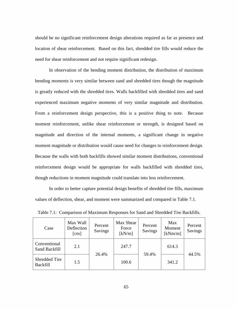
65
should be no significant reinforcement design alterations required as far as presence and
location of shear reinforcement. Based on this fact, shredded tire fills would reduce the
need for shear reinforcement and not require significant redesign.
In observation of the bending moment distribution, the distribution of maximum
bending moments is very similar between sand and shredded tires though the magnitude
is greatly reduced with the shredded tires. Walls backfilled with shredded tires and sand
experienced maximum negative moments of very similar magnitude and distribution.
From a reinforcement design perspective, this is a positive thing to note. Because
moment reinforcement, unlike shear reinforcement or strength, is designed based on
magnitude and direction of the internal moments, a significant change in negative
moment magnitude or distribution would cause need for changes to reinforcement design.
Because the walls with both backfills showed similar moment distributions, conventional
reinforcement design would be appropriate for walls backfilled with shredded tires,
though reductions in moment magnitude could translate into less reinforcement.
In order to better capture potential design benefits of shredded tire fills, maximum
values of deflection, shear, and moment were summarized and compared in Table 7.1.
Table 7.1: Comparison of Maximum Responses for Sand and Shredded Tire Backfills.
Case Max Wall Deflection
[cm]
Percent Savings
Max Shear Force
[kN/m]
Percent Savings
Max Moment [kNm/m]
Percent Savings
Conventional Sand Backfill
2.1
26.4%
247.7
59.4%
614.3
44.5% Shredded Tire Backfill
1.5 100.6 341.2

66
Here it can be seen that the reduction in maximum deflection for shredded tire
backfill was more than 25%. Reductions in shear force and moment induced in the wall
stem were even greater than the deflection reduction. This definitively shows that
shredded tire backfills, when the wall geometry is designed for them appropriately, can
not only reduce costs and amounts of materials for wall construction, fill, and excavation,
but can reduce demands on the retaining wall itself. As previously stated, this could
provide benefits in steel reinforcement requirements as well as creating less deflection
where sensitive structures may be affected.
In addition to comparing the behavior and performance of the wall, it is important
to note how shredded tire fills may affect ground responses and, as a result, structures
built on and near retained slopes that utilize shredded tire fills. A reduction in wall
deflection is a positive aspect from a settlement perspective, but base acceleration of
nearby structures or those associated with the wall itself is another important
consideration. To assess this, the spectral acceleration was observed for the top of the
backfill zone, top of the in-situ soil behind the backfill zone, and at the wall tip. These
acceleration spectra would be applied to design of structures that would be constructed in
these zones or be affected by the acceleration of the ground or wall structure. Plots of the
predicted accelerations are shown in Figure 7.4.
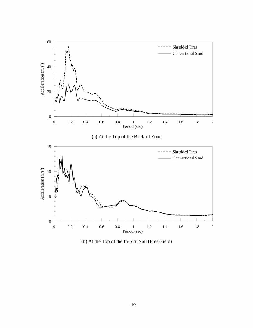
67
0 0.2 0.4 0.6 0.8 1 1.2 1.4 1.6 1.8 2Period (sec)
0
20
40
60A
ccel
erat
ion
(m/s
2 )Shredded Tires
Conventional Sand
(a) At the Top of the Backfill Zone
0 0.2 0.4 0.6 0.8 1 1.2 1.4 1.6 1.8 2Period (sec)
0
5
10
15
Acc
eler
atio
n (m
/s2 )
Shredded Tires
Conventional Sand
(b) At the Top of the In-Situ Soil (Free-Field)

68
0 0.2 0.4 0.6 0.8 1 1.2 1.4 1.6 1.8 2Period (sec)
0
10
20
30
40
50A
ccel
erat
ion
(m/s
2 )Shredded Tires
Conventional Sand
(c) At the Tip of the Wall
Figure 7.4: Spectral Accelerations Observed by Location Considering 5% Damping.
The first of these response spectra is applicable for structures with foundations
located within the backfill zone. Here we see that the amplitude of accelerations within
the backfill zone are greatly amplified by the shredded tire fills. This is most likely
attributed to the significantly lower modulus of shredded tire fills when compared to the
conventional sand fill. This could present a design complication if structures are to be
constructed in immediate proximity to the retaining structure. It is important to note,
however, that the backfill zone for the shredded tire fills is significantly smaller than that
of sand fills. This brings attention to the next graph, which shows the response spectra
for the “free-field” zone located within the in-situ material beyond the backfill zone.
Here the shredded tire fill did not greatly affect the amplitude of the accelerations and
only slightly affected the frequency content when compared with sand backfill. This

69
indicates that amplification of the acceleration response due to the use of shredded tire
backfill is largely isolated to the backfill zone near the wall. This is confirmed by
observation of the final plot of the spectral acceleration of the wall tip. Similar to the
response of the backfill zone, the acceleration response of the wall tip is amplified by the
use of shredded tire fill. These amplifications are important to note in the event that a
structure is expected to be located at these points, but do not pose a significant problem
anywhere beyond immediate proximity the wall.
Parametric Study on Variations in Shredded Tire Properties
In addition to evaluating the performance of shredded tires compared to
conventional fills, it was important to note that shredded tire properties tend to vary
greatly, specifically the friction angle, cohesion, and unit weight. These properties can
affect wall performance so it is important to evaluate how much effect on wall
performance is observed. Using the calibrated variations of the material properties and
the Hardening Soil model, wall tip deflections, shear forces, and bending moments were
observed for variations in shredded tire properties.
The first of these performance criteria was the deflection of the wall stem
throughout the dynamic loading. Deflection time histories are shown based on the
material property being varied in Figure 7.5. Shown for the friction angle is ±2σ because
the soil body collapsed in simulations where the friction angle was -3σ below the mean.
In addition, the cohesion value for -1σ was zero, forming the lower limit for this
variation.

70
0 2 4 6 8 10Dynamic Time (sec)
-2
-1
0
1
2
3W
all D
efle
ctio
n (c
m)
µφ+2σMean
µφ−2σ
(a) Effect of Variation of the Friction Angle
0 2 4 6 8 10Dynamic Time (sec)
-2
0
2
Wal
l Def
lect
ion
(cm
)
µc+3σMean
µc−1σ
(b) Effect of Variation of Cohesion

71
0 2 4 6 8 10Dynamic Time (sec)
-2
0
2W
all D
efle
ctio
n (c
m)
µγ+3σMean
µγ−3σ
(c) Effect of Variation of the Unit Weight
Figure 7.5: Deflection time histories of the wall stem for variation of each tire material property: HS Model-Damped
It can be seen from these graphs that variations in the material properties even as
much as three standard deviations above and below the mean had little effect on the
amplitude and frequency characteristics of the deflection. Generally, both increases and
decreases in the friction angle produced slightly higher deflections though generally by
only a small amount. Changes in the friction angle represent the greatest change in the
stiffness characteristics of the backfill and thus demonstrate the greatest apparent change
in the frequency characteristics of the deflection. A similar effect on the frequency of
deflection was noted in the variation of the cohesion properties of the backfill. Increases
in unit weigh appear to increase very slightly the amplitude of the wall deflection.
To understand better effects of material variation, the maximum values for
deflection, wall shear, and bending moment were determined for each variation and are

72
summarized in Table 7.2. Trends in maximum shear and moment values are also
represented graphically in the bar graphs in Figure 7.6.
Table 7.2: Summary of results from parametric study
Variable Case Max Wall
Deflection [cm] Max Shear
Force [kN/m] Max Moment
[kNm/m] Tires µ 1.23 100.66 341.20
Fric
tion
Ang
le µφ+3σ 2.24 122.25 444.90
µφ+2σ 1.40 98.16 338.69
µφ+1σ 1.38 99.78 342.18
µφ-1σ 1.32 94.56 347.41
µφ-2σ 1.34 108.47 366.70
µφ-3σ N/A N/A N/A
Coh
esio
n µc+3σ 1.28 109.85 359.65
µc+2σ 1.30 107.00 358.80
µc+1σ 1.33 103.55 357.54
µc-1σ 1.38 111.19 372.02
Uni
t Wei
ght
µγ+3σ 1.30 121.29 371.47
µγ+2σ 1.27 115.60 358.42
µγ+1σ 1.22 108.51 347.41
µγ-1σ 1.25 92.76 334.99
µγ-2σ 1.29 91.05 332.45
µγ-3σ 1.34 89.90 330.64
This maximum wall deflection represents the maximum deflection of the wall
away from the backfill material for consistency. Increases in wall deflection due to
increases in the friction angle can be attributed partially to the wall design. The extended
wall toe tends to put the backfill into more of a passive pressure situation, at least during
static loading which can mean that a higher friction angle would effectively increase the
wall pressure. Generally, however, changes in wall deflections with changes to the

73
material properties are minimal, even for changes in unit weight. Small and inconsistent
changes in the deflection response can likely be attributed to small changes in stiffness
and frequency characteristics and do not appear to present a great performance concern in
this case even the most extreme values are still less than 3 cm of deflection.
(a) Variation in the Max Shear Force
(b) Variation in the Max Bending Moment
Figure 7.6: Variation in maximum load from material property variations
0
20
40
60
80
100
120
140
+3σ +2σ +1σ µ -1σ -2σ -3σ
Max
She
ar F
orc
e (k
N/m
)
Case
Friction Angle Variation
Unit Weight Variation
Cohesion Variation
250
275
300
325
350
375
400
425
450
+3σ +2σ +1σ µ -1σ -2σ -3σ
Max
Ben
din
g M
om
ent
(kN
n/m
)
Case
Friction Angle Variation
Unit Weight Variation
Cohesion Variation

74
When observing trends in the shear and bending moment responses, there is
greater difference in the values for different variations in material properties. Similar to
the deflection response, the friction angle when at three standard deviations above the
mean showed the most dramatic increase in the shear force and bending moments. An
absence of cohesion also showed a more marked increase in both shear force and bending
moments in the wall. Otherwise, all shear force and bending moments hover around the
same value for both the friction angle and cohesion variations. Generally, increases in
unit weight induced greater forces and moments in the wall as was to be expected.
Generally variations in the three shredded tire properties being considered did not
cause significant changes in the wall response and on initial inspection seem to be well
within acceptable ranges for variations. In the following section, a reliability analysis is
performed to determine how variations in the friction angle, cohesion, and unit weight
manifest in changes in wall responses. The results of this analysis are detailed in the
following section.
Reliability Analysis of Parametric Study Results
In order to quantify the effects of the variations in shredded tire properties on wall
performance, the results from the parametric study were considered in a reliability
analysis. For this analysis, a simplified version of the First Order Second Moment
(FOSM) Method was used. This method allows for the determination of the mean and
standard deviation of responses to be determined when the function used to calculate the
response values is unknown or complex, as is the case with finite element analysis (Dang
et. al 2012, Juang et. al. 2009). Equations 12 and 13 are the two full equations used in the

75
FOSM Method to describe the mean (µd) and variance (σd2) of the response based on the
parameters being varied.
�� = ���� , ��� , ��, ������ (12)
�� = �������� + ���
������� + 2 ������ �
������ (�����) (13)
Here d = the wall tip deflection, γ = the unit weight of the shredded tires, ϕ = the
friction angle of the shredded tires, c’ = the cohesion of the shredded tires, xother = other
shredded tire input parameters, and ρ = the correlation coefficient between the two
variables being considered, here c’ and ϕ. Equation 12 describes the mean response as a
function of the properties of the shredded tires being varied in the parametric study.
Equation 13 gives the standard deviation of the response, here deflection, in terms of
variations in two of the properties, here friction angle and cohesion. In this study, the
mean response was evaluated using PLAXIS with the input of the mean shredded tire
properties. This equation can be simplified to achieve Equation 14, the one used in this
reliability study.
�� = ���� + ���� + 2�������� (14)
Here each of the d = the wall deflection and ∆� = ������������ �� ��������� �� �����������
�� . As
before, this shows the equation for the wall deflection in terms of the variation in the
cohesion and the friction angle of the shredded tire backfill, but this equation was
similarly used for other variable pairs and wall response criterion. The deflection
gradient (∆d), shear force gradient (∆V), and bending moment gradient (∆M) were
calculated according to the recorded responses from each of the variables considered. In

76
order to determine the correlation coefficient for each variable pair, the covariance
between the unit weight and cohesion, between the friction angle and the cohesion, and
between the unit weight and the cohesion were determined based on the values of these
variables obtained from the literature (see Chapter 6). Once the covariance values had
been determined for each pairing, the correlation coefficient for each pair was calculated
using the following equation.
=���,����� (15)
where v[x,y] = the covariance of the two variables in question and the σx,σy = the
standard deviation of each variable in the pair. The values for the covariance and
correlation for each pair of variables is shown in Table 7.3. This table also shows the
summary of all reliability values obtained from the reliability analysis of the results
obtained from PLAXIS simulations in the parametric study.
Table 7.3: Reliability analysis of data from the parametric study
Unit Weight and Friction Angle
Friction Angle and Cohesion
Unit Weight and Cohesion
Covariance ρ-value Covariance ρ-value Covariance ρ-value 1.274 0.329 -31.849 -0.550 -1.738 -0.267
Variation in Maximum Wall Deflection [cm] µd 1.228 µd 1.228 µd 1.228
σd 0.026 σd 0.022 σd 0.025
Variation in Maximum Shear Force[kN/m] µV 100.66 µV 100.66 µV 100.66
σV 7.670 σV 2.208 σV 6.183
Variation in Maximum Moment [kNm/m] µM 341.20 µM 341.20 µM 341.20
σM 9.274 σM 4.792 σM 6.494

77
Here, the values of the friction angle, cohesion, and unit weight were considered
since the variation of these parameters was known from the samples in the literature, but
it is important to note that though these values are correlated to the hardening soil
parameters being varied, they do not explicitly quantify all of the variations in the
properties in this study. Even so, since variations in the friction angle, cohesion, and unit
weight were used in the calibration of the other parameters, they are considered to be
perfectly correlated for the purpose of this reliability analysis.
The unit weight and friction angle tend to vary primarily with size and particle
shape and thus maintain a high correlation coefficient, greater than would probably be
expected for soils. Cohesion tends to vary with exposed metal content in shredded tire
chips which is often related to the size and because of this and the fact that both are shear
strength properties, is correlated with the friction angle. These values are also typically
highly correlated in soils so this correlation makes sense. Unit weight and cohesion are
not highly correlated because the only potential correlating factor between these two is
chip size relationships with exposed metal content.
As was observed in the viewing of the data from PLAXIS, the wall deflection has
a small variation with respect to all of the property variations and thus demonstrates a
very small standard deviation for this response parameter. Joint variation of the friction
angle and unit weight have the greatest effect on the shear force and bending moment
induced in the wall followed by unit weight and cohesion. This indicates that both
friction angle and unit weight have higher influences on the shear forces and moments
induced in the wall despite the fact that cohesion tends to be the most varied of the three

78
properties in shredded tire samples. Because these two parameters are primarily
governed by tire chip size and shape, both dependent on processing techniques, they
should be reasonably easy to control in construction. Based on these results, engineers
should be able to make decisions based on the friction angle, cohesion, and unit weight
characteristics, all of which are relatively to test, in order to select materials that will fit
within the allowable variations for their designs.

79
CHAPTER 8
EFFECTS OF CONSTITUATIVE MODELS ON COMPUTED RESPONSES
In addition to studies completed with the Hardening Soil model, similar
parametric studies were conducted to investigate the effect of different constitutive
models and the viscous damping. These parametric studies include Mohr-Coulomb
material model with no viscous damping and the Mohr-Coulomb material model with
viscous damping. These cases utilize the simpler Mohr-Coulomb material model, which,
while it is a less comprehensive material model, particularly for dynamic analysis,
provided the benefits of experimentally determined material properties from a wide range
of studies. In this chapter, the two material models are first compared for the mean
properties of the shredded tire backfill. Second, comparisons are made between the
damped and undamped site responses produced in the models that utilize the Mohr-
Coulomb material model. Lastly, a parametric study for the two Mohr-Coulomb cases is
considered and a reliability analysis is performed for each.
Variation in Response Due to Material Model and Damping
Because the behavior of shredded tires does differ from soils, it is important to
consider which material model is best for the modeling of shredded tires in finite element
analysis and, more importantly, in dynamic simulations. The Hardening Soil model is the
most robust and complex of the models considered in this study, particularly in the ability
to model loading and unloading and higher strains, but it is important to compare the
effects of using this model in comparison to the simpler Mohr-Coulomb Model. Though
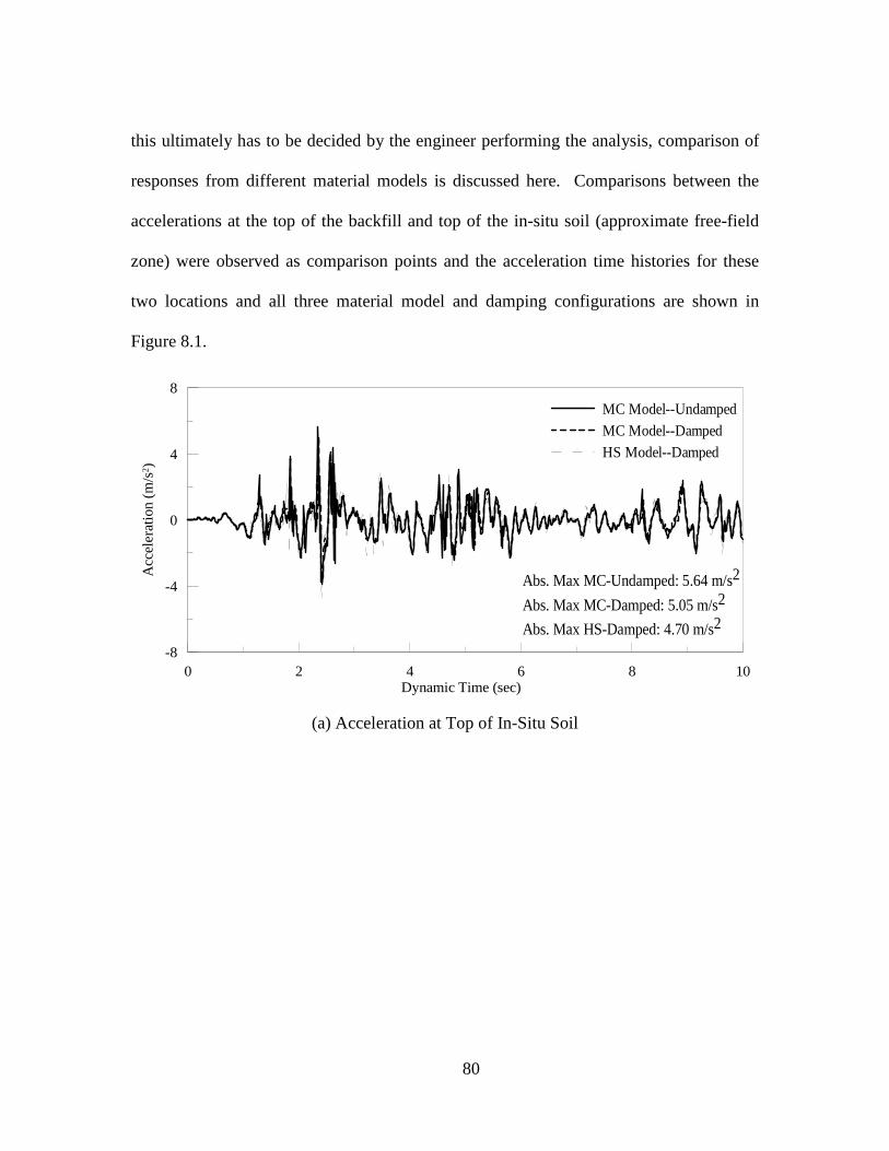
80
this ultimately has to be decided by the engineer performing the analysis, comparison of
responses from different material models is discussed here. Comparisons between the
accelerations at the top of the backfill and top of the in-situ soil (approximate free-field
zone) were observed as comparison points and the acceleration time histories for these
two locations and all three material model and damping configurations are shown in
Figure 8.1.
0 2 4 6 8 10Dynamic Time (sec)
-8
-4
0
4
8
Acc
eler
atio
n (m
/s2 )
MC Model--Undamped
MC Model--Damped
HS Model--Damped
Abs. Max MC-Undamped: 5.64 m/s2
Abs. Max MC-Damped: 5.05 m/s2
Abs. Max HS-Damped: 4.70 m/s2
(a) Acceleration at Top of In-Situ Soil

81
0 2 4 6 8 10Dynamic Time (sec)
-20
-10
0
10
20
Acc
eler
atio
n (m
/s2 )
MC Model--Undamped
MC Model--DampedHS Model--Damped
Abs. Max MC-Undamped: 17.60 m/s2
Abs. Max MC-Damped: 15.50 m/s2
Abs. Max HS-Damped: 12.95 m/s2
(b) Acceleration at Top of Shredded Tire Backfill
Figure 8.1: Comparisons of Acceleration Responses for HS Model and MC Models
Two main items can be noted from the acceleration results: first, the shredded tire
fills tend to amplify the accelerations somewhat more than the in-situ soil and second that
the addition of damping to the Mohr-Coulomb model and the addition of modulus
reduction with strain in the Hardening Soil model both decrease the acceleration
responses at both locations. Reductions in maximum acceleration caused by application
of damping the Mohr-Coulomb model was approximately 10-12% whereas reductions
from moving to the Hardening Soil model from the Mohr-Coulomb model varied more
between the locations. Based on realistic modeling criteria, damping is deemed
necessary as the system does experience some damping from particle friction as well as
hysteretic damping, which is not accounted for. It can also be acknowledged that
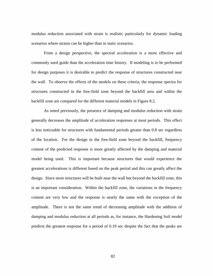
82
modulus reduction associated with strain is realistic particularly for dynamic loading
scenarios where strains can be higher than in static scenarios.
From a design perspective, the spectral acceleration is a more effective and
commonly used guide than the acceleration time history. If modeling is to be performed
for design purposes it is desirable to predict the response of structures constructed near
the wall. To observe the effects of the models on these criteria, the response spectra for
structures constructed in the free-field zone beyond the backfill area and within the
backfill zone are compared for the different material models in Figure 8.2.
As noted previously, the presence of damping and modulus reduction with strain
generally decreases the amplitude of acceleration responses at most periods. This effect
is less noticeable for structures with fundamental periods greater than 0.8 sec regardless
of the location. For the design in the free-field zone beyond the backfill, frequency
content of the predicted response is more greatly affected by the damping and material
model being used. This is important because structures that would experience the
greatest accelerations is different based on the peak period and this can greatly affect the
design. Since most structures will be built near the wall but beyond the backfill zone, this
is an important consideration. Within the backfill zone, the variations in the frequency
content are very low and the response is nearly the same with the exception of the
amplitude. There is not the same trend of decreasing amplitude with the addition of
damping and modulus reduction at all periods as, for instance, the Hardening Soil model
predicts the greatest response for a period of 0.19 sec despite the fact that the peaks are
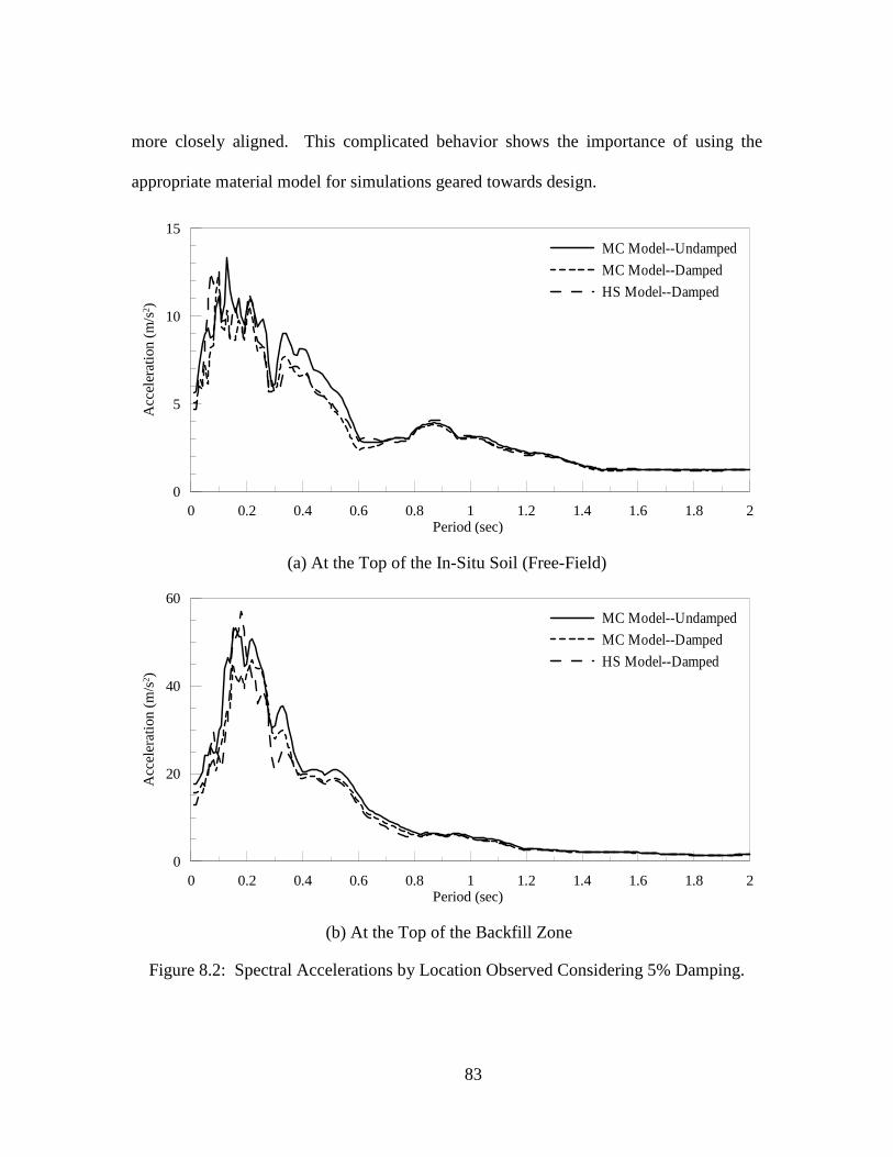
83
more closely aligned. This complicated behavior shows the importance of using the
appropriate material model for simulations geared towards design.
0 0.2 0.4 0.6 0.8 1 1.2 1.4 1.6 1.8 2Period (sec)
0
5
10
15
Acc
eler
atio
n (m
/s2 )
MC Model--Undamped
MC Model--Damped
HS Model--Damped
(a) At the Top of the In-Situ Soil (Free-Field)
0 0.2 0.4 0.6 0.8 1 1.2 1.4 1.6 1.8 2Period (sec)
0
20
40
60
Acc
eler
atio
n (m
/s2 )
MC Model--Undamped
MC Model--Damped
HS Model--Damped
(b) At the Top of the Backfill Zone
Figure 8.2: Spectral Accelerations by Location Observed Considering 5% Damping.

84
It is important to keep in mind that these comparisons merely compare the
material models to each other and note the effects of damping on the response but do not
compare any of the models to actual measurements. In order to determine which model
is most appropriate, the material model needs to be compared to experimental results and
damping must be estimated as best as possible.
Mohr-Coulomb Model without Rayleigh Damping
To investigate the effects of constitutive models and damping on the response,
parametric studies similar to those described in Chapter 7 for the Hardening Soil model
were similarly performed using the Mohr-Coulomb material model. The first study
utilized the Mohr-Coulomb material model with no external damping applied. The first
output of interest was the wall deflection time history, which is computed by observing
relative displacements of the wall tip and the wall base. The wall deflection time
histories for each property variation are shown in Figure 8.3.
(a) Effect of Variation of the Friction Angle
0 2 4 6 8 10Dynamic Time (sec)
-2
0
2
4
Wal
l Def
lect
ion
(cm
)
µφ+3σMean
µφ−3σ

85
(b) Effect of Variation of Cohesion
(c) Effect of Variation of the Unit Weight
Figure 8.3: Deflection time histories of the wall stem for variation of each tire material property: Undamped M-C Model
First, Figure 8.3(a) shows the deflection time histories for the mean shredded tires
compared to that for shredded tires with varying friction angles at three standard
deviations above and below the mean. This plot shows that the friction angle variation
produces only a small variation in the response, which is difficult to distinguish
graphically during much of the dynamic loading, but that the shredded tires with higher
friction angle produce a greater deflection in a wall than shredded tires with a lower
0 2 4 6 8 10Dynamic Time (sec)
-2
0
2
4W
all D
efle
ctio
n (c
m) µc+3σ
Mean
µc−1σ
0 2 4 6 8 10Dynamic Time (sec)
-2
0
2
4
Wal
l Def
lect
ion
(cm
)
µφ+3σMean
µφ−3σ

86
friction angle. Figure 8.3(b) similarly shows the variation in the wall deflection time
history as the cohesion of the shredded tire backfill is varied. Because the µc’-1σ case has
a cohesion value of 0, it is the lowest cohesion tested and is included in Figure 8.3(b).
Again, the cohesion of the shredded tires does not cause a dramatic change in the wall
behavior except in the µc’-1σ case where the cohesion is 0. It is noted that a lack of
cohesion reduces the amount of deflection in the wall for almost the entire loading cycle,
whereas the increased cohesion slightly increases the wall deflection. Next, Figure 8.3(c)
shows the effect on the wall deflection time history as the unit weight of the tires is
varied. Again, this shows no dramatic change in the wall response based on variation in
the unit weight, but shredded tires with a lower unit weight do produce slightly lower
wall deflections.
To get a better idea of trends in the wall response, quantitative maximums for the
criteria of interest were obtained as shown in Table 8.1. In addition, in order to see the
trends in the maximum shear and moment on the wall for each case and to compare the
effects of the variables, the bar charts in Figure 8.4 were plotted for in the information in
Table 8.1. This analysis shows a consistent trend in all of the response criteria for
variations in the fiction angle and cohesion: reductions in the shear strength parameters
produce less deflection, lower shear force, and lower bending moments in the wall stem.
This is probably due to the unorthodox wall dimensions necessary to accommodate the
shredded tire properties in seismic design particularly the long toe and short heel that
result from the lightweight of the shredded tires. The resulting eccentricity of such a wall
is on the heel side of the center, unlike in conventional walls, causing the wall to tend to
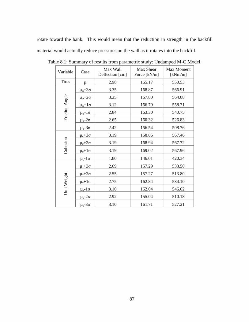
87
rotate toward the bank. This would mean that the reduction in strength in the backfill
material would actually reduce pressures on the wall as it rotates into the backfill.
Table 8.1: Summary of results from parametric study: Undamped M-C Model.
Variable Case Max Wall
Deflection [cm] Max Shear
Force [kN/m] Max Moment
[kNm/m]
Tires µ 2.98 165.17 550.53
Fri
ctio
n A
ngle
µφ+3σ 3.35 168.87 566.91
µφ+2σ 3.25 167.80 564.08
µφ+1σ 3.12 166.70 558.71
µφ-1σ 2.84 163.30 540.75
µφ-2σ 2.65 160.32 526.83
µφ-3σ 2.42 156.54 508.76
Coh
esio
n µc+3σ 3.19 168.86 567.46
µc+2σ 3.19 168.94 567.72
µc+1σ 3.19 169.02 567.96
µc-1σ 1.80 146.01 420.34
Uni
t Wei
ght
µγ+3σ 2.69 157.29 533.50
µγ+2σ 2.55 157.27 513.80
µγ+1σ 2.75 162.84 534.10
µγ-1σ 3.10 162.04 546.62
µγ-2σ 2.92 155.04 510.18
µγ-3σ 3.10 161.71 527.21

88
(a) Variation in the Max Shear Force
(b) Variation in the Max Bending Moment
Figure 8.4: Variation in maximum wall load based on material property variations: Undamped M-C Model
130
135
140
145
150
155
160
165
170
175
+3σ +2σ +1σ µ -1σ -2σ -3σ
Max
She
ar F
orc
e (k
N/m
)
Case
Friction Angle Variation
Unit Weight Variation
Cohesion Variation
400
425
450
475
500
525
550
575
600
+3σ +2σ +1σ µ -1σ -2σ -3σ
Max
Mo
men
t (k
Nn/
m)
Case
Friction Angle Variation
Unit Weight Variation
Cohesion Variation

89
Mohr-Coulomb Model with Rayleigh Damping
In the next parametric study, the shredded tire properties were varied as before
using the Mohr-Coulomb material model, but in this case, external Rayleigh damping
was utilized in the modeling of the shredded tires and the in-situ soil. The values for the
Rayleigh damping parameters were determined as previously described, and the addition
of damping was believed to give a more realistic response. In addition to being used in a
parametric comparison, these results can be compared to the results from the undamped
case and the Hardening Soil model study to see the effects of the constitutive model and
damping schemes. As with the previous parametric study, the wall deflection time
history, maximum wall deflection, maximum shear force in the wall, and the maximum
bending moment in the wall were observed for each of the variations in the shredded tire
friction angle, cohesion, and unit weight.
First, Figure 8.5 shows the wall deflection time histories for variations in the
shredded tire properties. As noted in other studies, wall deflection amplitude and
frequency content are not greatly affected by the variation of these parameters. Upon
inspection of these graphs and cases, changes in the unit weight of the shredded tire
backfill seemed to make the most profound difference in the deflection response of the
wall. As noted previously, increases in the unit weight generally increase the amplitude
of the wall deflection though still only very slightly. It can generally be said that the wall
stem is sufficiently stiff as to not be greatly impacted by the shredded tire property
variations.

90
(a) Effect of Variation of the Friction Angle
(b) Effect of Variation of Cohesion
(c) Effect of Variation of the Unit Weight
Figure 8.5: Deflection time histories of the wall stem for variation of each tire material property: Damped M-C Model
0 2 4 6 8 10Dynamic Time (sec)
-2
-1
0
1
2
3W
all D
efle
ctio
n (c
m)
µφ+3σMean
µφ−3σ
0 2 4 6 8 10Dynamic Time (sec)
-2
0
2
4
Wal
l Def
lect
ion
(cm
) µc+3σMean
µc−1σ
0 2 4 6 8 10Dynamic Time (sec)
-2
0
2
4
Wal
l Def
lect
ion
(cm
) µγ+3σMean
µγ−3σ
91
In addition to the graphical representation above, the maximum wall deflections,
shear forces, and bending moments in the wall for the dynamic loading are summarized
in Table 8.2. This summary confirms that there is very little if any apparent effect on the
wall deflection due to variations in the shredded tire properties. The primary difference
in the results from this model and others is that the shear and moment are generally
decreased by increases in shear strength parameters. Trends in the shear and bending
moments in the wall can be seen more clearly in the bar graphs in Figure 8.6.
Table 8.2: Summary of results from parametric study: Damped M-C Model.
Variable Case Max Wall
Deflection [cm] Max Shear
Force [kN/m] Max Moment
[kNm/m]
Tires µ 2.39 152.18 488.20
Fri
ctio
n A
ngle
µφ+3σ 2.32 134.99 456.60
µφ+2σ 2.34 140.51 466.38
µφ+1σ 2.36 146.31 477.01
µφ-1σ 2.42 157.71 499.78
µφ-2σ 2.45 162.39 511.51
µφ-3σ 2.49 166.94 522.70
Coh
esio
n µc+3σ 2.38 153.38 489.20
µc+2σ 2.38 153.38 489.20
µc+1σ 2.38 153.19 489.08
µc-1σ 2.04 148.34 426.53
Uni
t Wei
ght
µγ+3σ 2.64 164.97 509.01
µγ+2σ 2.37 160.83 488.69
µγ+1σ 2.38 155.05 486.45
µγ-1σ 2.39 148.15 490.94
µγ-2σ 2.32 137.26 481.81
µγ-3σ 2.54 128.92 457.54

92
(a) Variation in the Max Shear Force
(b) Variation in the Max Bending Moment
Figure 8.6: Variation in maximum wall load based on material property variations: Damped M-C Model
These graphs show very little variation in the shear force values for variations in
shear strength parameters except that increasing the cohesion and friction angle generally
decrease demand on the wall, even if only slightly. Unit weight shows somewhat more
0
25
50
75
100
125
150
175
200
225
+3σ +2σ +1σ µ -1σ -2σ -3σ
Max
She
ar F
orc
e (k
N/m
)
Case
Friction Angle Variation
Unit Weight Variation
Cohesion Variation
300
325
350
375
400
425
450
475
500
525
550
575
+3σ +2σ +1σ µ -1σ -2σ -3σ
Max
Ben
din
g M
om
ent
(kN
n/m
)
Case
Friction Angle Variation
Unit Weight Variation
Cohesion Variation
93
influence on the shear and bending moments, with increases in the unit weight generally
increasing the shear and moment in the wall as is to be expected. These results show
more concrete trends in how the parametric variation affects the wall response than the
undamped case, which generally agrees with the idea that the addition of damping is
necessary to get a realistic response. The trends in the response are simpler than those
observed for the Hardening Soil model, as the Mohr-Coulomb model is a more simplistic
method in general for modeling soil behavior. Determination of the best material model
and damping scheme for use with shredded tire fills warrants further study.
94
CHAPTER 9
CONCLUSIONS AND FUTURE WORK
At the conclusion of such intensive modeling of the retaining wall with varying
backfill materials, many observations can be made and many questions have been
clarified and raised as a result. This section serves as a summary of the conclusions
drawn from the results and outlines what future work needs to be completed to
understand better how shredded tires perform as a retaining wall backfill in seismic
zones.
Conclusions
Generally, shredded tire fills showed excellent performance benefits when
compared to conventional sand fills. Shredded tires are low-cost, lightweight, recycled,
and sustainable and this research combined with previous studies and field trials shows
that they are a viable alternative fill in this application. In design, they reduce wall size,
heel length, and resulting excavation and fill quantities. These all can present an upfront
cost savings in addition to the fact that shredded tires generally have a lower unit cost
than conventional fills when borrow is required. In performance analyses, both materials
were testing in conjunction with walls specifically designed for implementation with a
particular fill material and shredded tires presented great reductions in wall deflection
(both dynamic and permanent static) and decreases in the maximum shear and moment
demands on the wall structure. Additionally it was shown that shredded tires do not
significantly change the distribution of maximum positive and negative shears and

95
moments in ways that would require changes to conventional structural design methods.
This positive performance indicates that shredded tires appear to be a viable alternative to
conventional sand fills for many retaining wall applications in seismic zones.
Parametric studies of shredded tire backfill performance and subsequent
reliability study showed that variations in shredded tire properties generally caused little
variation in wall performance in terms of deflection, shear force, and bending moment.
Friction angle and unit weight variations seemed to cause the greatest variation in the
shear and bending moment in particular. This observation was extended to say that
because these properties vary primarily with the size and shape of tire shreds, that
variation in these properties and the resulting variations in wall demands could largely be
controlled by monitoring of tire shred size and manufacturing processes in construction
processes. Other methods for keeping consistent and expected values for friction angle
and unit weight could include methods of compaction and other construction controls.
Regarding the effects of constitutive modeling of shredded tire and soil systems,
the minimum requirement is the application of reasonable Rayleigh damping to all
models. Ideally, this would be accompanied by a material model, such as the Hardening
Soil model, that can describe the behavior of shredded tires. Because soil models may
not be ideal for modeling shredded tires due to elastic particle behavior and other
considerations, it is best to base material model effectiveness on experimental lab testing
(both dynamic and static in ideal cases) to determine the best model and input parameters
to get realistic results. The Hardening Soil model seems like a reasonable model that
improves on the more simplistic Mohr-Coulomb material model and takes into account

96
the modulus reduction of shredded tires and soils. Ultimately, this brings up the question
of the best material model to use, which requires more comprehensive study and
correlation between experimentally observed behaviors and fit of different material
models.
Practical Application of this Research
The research performed here is ideally helpful in real-world design applications.
If shredded tires are to be used as a fill material, their benefits can most ideally be
realized by designing the wall to optimize the different properties of shredded tire fills.
This study identified some features that can improve wall performance and economy with
the use of shredded tire fills with specific design modifications such as a lengthened wall
toe and shortened wall heel. On the other hand, these design modifications are a
consideration for some projects where excavation or clearance in front of the wall could
be a concern, so it is important to note this. With the designs in this study as a guide,
however, it is possible to get the most benefit from the use of shredded tire fills.
Recommendations for Future Work
The first recommendation for further study stems from the difficulties and
uncertainties associated with material modeling. In order to gain more in-depth modulus
characteristics for shredded tires, cyclic triaxial tests are warranted. These tests should be
performed for a large but reasonable range of shredded tire sizes and types and care
should be taken to accommodate the increased particle size by using a larger triaxial cell.
These types of tests could provide the loading and unloading modulus values and better

97
characterize the modulus reduction associated with high strains. Due to compressibility
of rubber particles, moduli must also take into account the deformation of these particles
and material models must satisfactorily consider this. Soil material models generally
only consider interactions between particles but do not allow for particle deformation.
This could be dealt with by determining shear moduli and elastic moduli through
independent tests and allowing each to encompass the effects of particle moduli. The
elastic range of the shredded tires is already known to be larger than that of soils due to
the elasticity of rubber particles. This characteristic could have great effects on the
response, particularly in dynamic response, and should be accounted for in the modulus
and failure criterion provided for any material model.
Outside of material lab tests, full-scale tests are also recommended both static and
dynamic. Some static full-scale applications have been studied and could be augmented
by the addition of dynamic loads. This would best be approximated by use of a shake
table with a full-scale retaining wall model. Comparison of the response observed in
scale models should be compared to responses predicted using the material modeling
techniques based on material properties previously described. Instrumentation of the
scale models should include observations of the wall response as well as settlement of the
surface and within the shredded tire fill. All studies should also be extended to include
surcharge loads and/or sloped backfills if possible.
In terms of reliability analysis, further study is recommended to improve upon the
FOSM methods used here. Though FOSM estimations were most practical given the
amount of information available, Monte Carlo simulation would be ideal and could be

98
made even more effective when based on information gained from further material
testing. Only through Monte Carlo simulation could the effects of material variation be
fully understood.

99
APPENDICES

112
REFERENCES
American Society for Testing and Materials (2008). ASTM D6270-08: Standard Practice for Use of Scrap Tires in Civil Engineering Applications.
Anderson, D.G., Martin, G.R., Lam, I.P., & Wang, J.N. (2008) NCHRP Report: 611:
Seismic Analysis and Design of Retaining Walls, Buried Structures, Slopes, and Embankments. Transportation Research Board Project 12-70.
Byung Sik, C., Kyung Min, K., & Ki Deok, M. (2004). A Study on Reliability Analysis
for Reinforced Earth Retaining Walls. 3rd Asian Regional Conference on Geosynthetics, 248-254. GeoAsia.
Cecich, V., Gonzales, L., Hoisaeter, A., Williams, J., & Reddy, K. (1996). Use of
Shredded Tires as Lightweight Backfill Material for Retaining Structures. Waste Management & Research, 14, 433-451.
Chien, Y.-C., Ton S., Lee, M.-H., Chia, T., Shu, H.-Y., & Wu, Y.-S. (2003). Assessment
of occupational health hazards in scrap-tire shredding facilities. The Science of the Total Environment, 309 (1-3), 35-46. doi: 10.1016/S0048-9697(03)00009-3
Dang, H-P., Lin, H-D., & Juang, C.H. (2012). Evaluation of Soil Variability Influence on
Deep Excavation Analysis—Simplified Approach. GeoCongress 2012, 2895-2903.
Eldin, N.N., & Piekarski, J.A. (1993). Scrap Tires: Management and Economics.
Journal of Environmental Engineering, 119 (6), 1217-1232. Humphrey, D.N., Sandford, T.C., Cribbs, M.M., & Manion, W.P. (1993). Shear Strength
and Compressibility of Tire Chips for Use as Retaining Wall Backfill. Transportation Research Record, 1422, 29-35.
Juang, C.H., Sunny Y.F., Tang, H.T., Khor, E.H., Kung, G.T-C., & Zhang, J. (2009).
Evaluating Model Uncertainty of an SPT-Based Simplified Method for Reliability Analysis for Probability of Liquefaction. Soils and Foundations, 49(1), 135-152.
Kaggwa, W.S. (2005). Probability-Based Diagnosis of Defective Geotechnical
Engineering Structures. Journal of Performance of Constructed Facilities, 19(4), 308-315. doi: 10.1061/(ASCE)0887-3828(2005)19:4(308).

113
Khan, A. A., Karanfil, T., & Grayson, J. M. (2010). Septic Tank Tire Chip Study: The Feasibility of Tire Chips as a Substitute for Stone Aggregate in Septic Tank Leach Fields.
Lee, J.H., Salgado, R., Bernal, A., & Lovell, C.W. (1999). Shredded Tires and Rubber Sand as Lightweight Backfill. Journal of Geotechnical and Geoenvironmental Engineering, 125 (2), 132-141.
Lee, H.J. & Roh, H.S. (2007). The use of tire chips to minimize dynamic earth pressure
during compaction of backfill. Construction and Building Materials, 21, 1016-1026. doi: 10.1016/j.conbuildmat.2006.02.003.
Moo-Young, H., Sellasie, K., Zeroka, D., & Sabnis, G. (2003). Physical and Chemical
Properties of Recycled Tire Shreds for Use in Construction. Journal of Environmental Engineering, 129 (10), 921-929. doi: 10.1061/(ASCE)0733-9372(2003)129:10(921)
Nevada Department of Transportation (2001). Standard Specifications. Nevada Department of Transportation (2007). Types 1A & 1B Cantilever Concrete
Retaining Walls. Standard Plans. Nightingale, D.E.B., & Green, W.P. (1997). An Unsolved Riddle: Tire Chips, Two
Roadbeds, and Spontaneous Reations. ASTM Special Technical Publication, 1275 (Sept. 1997), 265-285.
Regional Transportation Commission of Southern Nevada (2010). Section 207: Structure
Backfill. Uniform Standard Specifications for Public Works Construction Off-Site Improvements (3rd ed.), 105-108. Las Vegas, Nevada: Uniform Standard Specifications Subcommittee.
S&ME (2010). Subsurface Exploration: West Abutment Replacement Saluda Drive at
Big Brushy Creek, Anderson County, SC. S&ME Project No. 1261-10-069. Report Prepared by Michael Revis, P.E. & David Swoap, P.E. (April 9, 2010).
Shalaby, A., & Khan, R.A. (2005). Design of unsurfaced roads constructed with large-
size shredded rubber tires: a case study. Resources, Conservation and Recycling, 44, 318-332. Doi: 10.1016/j.resconrec.2004.12.004
Sheehan, P.J., Warmerdam, J.M., Ogle S., Humphrey, D.N., & Patenaude, S.M. (2006).
Evaluating the Risk to Aquatic Ecosystems Posed by Leachate from Tire Shred Fill in Roads Using Toxicity Tests, Toxicity Identification Evaluations, and Groundwater Modeling. Environmental Toxicology and Chemistry, 25 (2), 400-411.

114
Tandon, V., Velazco, D.A., Nazarian, S., & Picornell, M. (2007). Performance Monitoring of Embankments Containing Tire Chips: Case Study. Journal of Performance of Constructed Facilities, 21 (3), 207-214. doi: 10.1061/(ASCE)0887-3828(2007)21:3(207)
Tawfik, E.F., Tariq, B.H., & Aggour, M.S. (2007). Design of Cantilever Retaining Walls
in Unsaturated Soils Using AASHTO Load and Resistance Factor Design (LRFD) Method. Proceedings of Sessions of Geo-Denver 2007 Congress: Probabilistic Applications in Geotechnical Engineering. Geotechnical Special Publication, 170, 57-66. Denver, CO: American Society of Civil Engineers. doi: 10.1061/40914(233)6
Visone, C., & Santucci de Magistris, F. (2008). A review of design methods for retaining structures under seismic loadings. Strategies for reduction of seismic risk (G. Fabbrocino & F. Santucci de Magistris eds.) pp. 51-64.
Warith, M.A., Evgin, E., & Benson, P.A.S. (2004). Suitability of shredded tires for use
in landfill leachate collection systems. Waste Management, 24, 967-979. doi: 10.1016/j.wasman.2004.08.004
Yang, S., Lohnes, R.A., & Kjartanson, B.H. (2002). Mechanical Properties of Shredded
Tires. Geotechnical Testing Journal, 25 (1), 44-52. Youwai, S., & Bergado, D.T. (2003). Strength and deformation characteristics of
shredded rubber tire-sand mixtures. Canadian Geotechnical Journal, 40, 254-264. doi: 10.1139/T02-104