notes on 22.76/3.s75 ionics and its applications
TRANSCRIPT
Notes on 22.76/3.S75 Ionics and Its
Applications
Ju Li, MIT, December 21, 2021
1 Electrostatics and Electrochemical Potential 3
1.1 Coulomb Explosion argument: bulk electroneutrality principle . . . . . . . . 6
1.2 Parallel Capacitor . . . . . . . . . . . . . . . . . . . . . . . . . . . . . . . . . 7
1.3 Equalization of Price: electronic versus ion/atom pair . . . . . . . . . . . . . 9
1.4 Electrocapillarity and Point-of-zero-charge (PZC) . . . . . . . . . . . . . . . 16
2 Electrons and Valence 20
3 Solvation Model and Debye–Huckel Equation 27
4 Electrode Kinetics 33
4.1 Butler-Volmer and Exchange Current Density . . . . . . . . . . . . . . . . . 34
4.2 Tafel Approximation . . . . . . . . . . . . . . . . . . . . . . . . . . . . . . . 38
4.3 Exchange current density and limiting curent density . . . . . . . . . . . . . 38
5 Long-range Mass Transport 39
1
5.1 Binary-Salt Liquid Electrolyte . . . . . . . . . . . . . . . . . . . . . . . . . . 42
5.2 Electrorefinning Example . . . . . . . . . . . . . . . . . . . . . . . . . . . . . 44
5.3 1D Cation Transport without Convection . . . . . . . . . . . . . . . . . . . . 47
5.4 Supporting Electrolyte . . . . . . . . . . . . . . . . . . . . . . . . . . . . . . 52
5.5 Convective Mass Transfer . . . . . . . . . . . . . . . . . . . . . . . . . . . . 53
5.6 Concentration Overpotential . . . . . . . . . . . . . . . . . . . . . . . . . . . 56
A Review of Bulk Thermodynamics 58
B Interfaces 84
B.1 Interfacial Segregation . . . . . . . . . . . . . . . . . . . . . . . . . . . . . . 84
B.1.1 McLean Isotherm for Interfacial Segregation . . . . . . . . . . . . . . 93
B.2 Wulff stability analysis . . . . . . . . . . . . . . . . . . . . . . . . . . . . . . 96
B.3 Gradient Thermodynamics Description of the Interface . . . . . . . . . . . . 101
C Neuromorphic equivalent circuit - Mantao model 106
C.1 Variable resistor solution . . . . . . . . . . . . . . . . . . . . . . . . . . . . . 110
2
Chapter 1
Electrostatics and Electrochemical
Potential
In this course we will examine the consequences of mobile ions and their valence changes
in liquids and solids. Ionics defined as such are crucial for various energy technologies (ET),
such as corrosion, batteries, fuel cells, electrolyzers, etc., with electrolytes ranging from liquid
water, organics, molten salts to solid electrolytes. Ionics are essential in biology, and may
even have information technology (IT) applications. [1]
Liquids and solids belong to so-called condensed-matter phases. In terms of thermodynamic
formulation, once solid-state diffusion is feasible at high enough temperature (T > TMelt/2
where TMelt is the bulk melting point of the solid), the treatment of ions in liquids and solids
are surprisingly similar in some aspects, as well as between mobile ions and electrons.
Also, solid grain boundaries and surfaces can often be thought of as “2D liquids” at such
temperatures. In terms of kinetics, liquids are generally faster than solids, but not always.
For example, Li+ cation moves surprisingly rapidly in some solid oxide or sulfide “superionic”
conductors [2], even faster than in liquid organics, because the Li+-sublattice is effectly
molten.
Electronics, namely mobile free electrons in metals and semiconductors, is driving the electri-
cal grid, TV and massaging chair, and computer farms. Ion is basically a nuclide surrounded
by some electrons (how many determines the valence of the ion). Therefore Ionics and
Electronics can be intimately related.
3
The electrons associated with an ion are bound, unless the ion undergoes a valence change,
or “redox” reaction (reduction/oxidation in chemistry lingo). It might be confusing that
sometimes “redox” reaction happens without any oxygen participating or even present. So
the word “oxidation” is a semantic overload and has double meaning depending on the
context.
The narrow meaning, as in “oxidation of my tin roof”, is the reaction of O2(g) and Sn(solid)
– but you might be surprised how often metals, especially at high temperatures, react with
H2O as well, as H2O can be a powerful oxidant, shown by the Ellingham diagram. In this
narrow definition of oxidation, we are talking about a standard chemical reaction, where
there is short-range electron transfer.
The broad meaning, as in “oxidation of my electrolyte”, is the molecules of my electrolyte
losing their bound electron. This electron can go to a metal current collector, and through
metal wiring, transferred to somewhere far away. Losing orignally-bound electrons is
the essence of oxidation. Gaining bound electrons is the essence of reduction.
In the nomenclature above, we need a criterion to distinguish between “free” and “bound”,
and “short-range” versus “long-range” transport. In this course, “short-range” and “bound”
means Angstrom-level. For example, in a pure dielectric material, under external electric
displacement field D, the bound charges in a molecule like H2O can shift sub-Angstrom
distance, but they cannot separate, and therefore D = ε0E + P = ε0(1 + χ)E = εrε0E,
where εr ≥ 1 is the dielectric constant, and ε0 = 8.8541878128E − 12 Farad/meter is the
vacuum permittivity. Since P screens D by a finite ratio, the response of the material tries to
cancel the external influence, but can only be successful to a finite factor. This is very
different when there are free electrons/ions in the medium (finite ionic strength). Free
electrons/ions can move an indefinite distance: given enough time, it can move centimeters or
even km, and they will inexorably try to not only screen the field, but to kill the field.
So external electric field cannot penetrate a semi-infinite metal or electrolyte indefintiely.
An electrolyte is a liquid or solid that can conduct certain kinds of free ions, but not free
electrons (naked). In contrast, a metal or semiconductor can conduct naked free electrons.
Since the effective mass of naked free electrons in a metal or semiconductor crystal:
m∗ ≡ h2/(∂2En(k)/∂k2) (1.1)
is often on the order of me, which is much smaller than the mass of ions (more on what is the
structure of an ion later), ionics will generally be slower than electronics. On the triangle of
4
dieletric - electrolyte - metal: deionized (DI) water is closer to the dieletric corner since
the ionic strength is on the order of 10−7M, 1M KOH solution is closer to the electrolyte
corner. Incidentally, water can indeed absorb electron, forming so-called “solvated electron”
[3], but the wavefunction of this electron will be localized, surrounded by water molecules,
and can be aptly called a polaron. This is unlike the band electron in semiconductor or
metallic crystals, with delocalized wavefunctions (think of a wavepack with 100nm extent).
So electronic conduction can either be ballistic (band-like delocalized electron) or hopping
(localized electron) that requires thermal activation. The latter kind of electron-conduction
mode is called polaron hopping mechanism.
Since we will be dealing with charges in Ionics, we need to talk about some peculiarities
about electrostatics
∇2φ(x, t) = −ρtotal(x, t)
ε0(1.2)
where φ(x) is the electrostatic potential,
ρtotal(x, t) = ρfree(x, t) + ρbound(x, t) (1.3)
where in the case of a water-solvent solution, ρbound(x, t) would be the charge distribution
due to undissociated water molecule, and ρfree(x, t) would be from the hydronium [H+],
the hydroxide [OH−], other cations and anions like [Na+], bicarbonate [HCO−3 ], and even
solvated electrons [e−]. ρtotal(x) is just a bunch of delta functions:
ρtotal(x, t) =∑
zkeδ(x− xk(t)) (1.4)
where k covers both nuclide and electrons, and e ≡ 1.60217662E−19 Coulomb. The “naked”
Poisson’s equation (1.2) is always true, at least in our class of Ionics (where one ignored the
magnetic induction term that gives ∂2t φ(x, t) and the speed of light, so Poisson’s equation is
instantaneous and thus all-covering spatially, an effect we will come to appreciate soon).
It turns out that one can sometime coarse-grain away the response the bound-charge solvent
(undissociated water molecules) and write down:
∇2φ(x, t) = −ρfree(x, t)
εrε0(1.5)
where εr = 78.4 for undissociated water solvent, and thus one only needs to regard the
free species. The caveat is that x should be “smeared out” and a few Angstroms away
5
from the details of the free charge location, and one needs to give enough time for the
undissociated water molecule to adjust, so the εr = 78.4 is actally so-called zero-frequency
dielectric constant. Then, both 1.2 and 1.5 can be formally written as
∇2φ = −ρε
(1.6)
One just need to be aware that things not written down do exist, and it’s important to keep
in mind the context and the approximations behind.
Let us put in some numbers. With 1 Angstrom distance, two elementary charges in vacuum
would incur
e2
4π × 8.8541878128E − 12× 1E − 10= 2.307077552341736E− 18J = 14.4eV (1.7)
interaction energy. If the same two charges are inside liquid water, with dielectric screening,
the interaction energy would be 18.37 meV across 1 nm distance.
1.1 Coulomb Explosion argument: bulk electroneutral-
ity principle
We next show that the coarse-grained free-charge density ρfree(x, t) cannot accumulate in an
infinte volume at finite uniform density
ρfree(x, t) = ρ0 6= 0, (1.8)
In other words, one cannot be in an infinite cloud of net-monopoles. This is because the
total electrostatic energy is
Etotal =1
2
∫ρ0dx
∫ρ0dx
′ 1
4πε(|x′ − x|)(1.9)
If we fix x, the inner integral is still divergent, as
∫ ∞0
dr4πr2 1
4πr(1.10)
6
is OK for the lower radial cutoff, but would diverge at upper cutoff. So the electrostatic
energy per volume would be +∞, and in such case, would lead to so-called Coulomb
Explosion. This actually happens when laser shines on a material and evaporates its
electrons very quickly.
The above means one cannot have k = 0 component to the total charge density. On the
other hand, other finite k components are OK, as one can Fourier transform ρfree(x, t) into
ρfree(x, t) =∑k 6=0
ρkeik·x (1.11)
but the smaller |k| is, the energetically more expensive this will be. This leads to the following
Parallel Capacitor model.
1.2 Parallel Capacitor
How about a wall of same-signed charges, separated by a wall of counter-charges across
distance d, like in the classic parallel-plate capacitor? Suppose each plate has area A = L2,
with L d, and the total charge in one wall is Q (the areal charge density is Q/A). The
classic electrostatics says that
∇ · E =ρ
ε(1.12)
since E ≡ −∇φ, and so the electric inside the capacitor would be Q/Aε. The + wall would
therefore has a higher electrostatic potential than the - wall, by
U =Qd
Aε(1.13)
and one can define capacitance as
C ≡ Q
U=Aε
d(1.14)
and so the larger the A, the larger the capacitance. On the other hand, the smaller the d, the
larger the capacitance also, according to 1.14. But this needs some careful understanding.
First, the medium in between cannot leak charge, i.e. it has to be a perfect dielectric (at
least resisting the range of U we will put on the capacitor). Secondly, this is only if the
coarse-graining of ε = εrε0 works, and this means d cannot be too small. With a very small
7
d both assumptions would come into severe trouble. The contiuum coarse-graining would
break down if d is a few angstroms (water O-H bond length is 0.96 A). Furthermore, the
small the d and the larger the E, the closer one would be near the dielectric breakdown
field strength Eds, and the more likely the “dam” would leak. If the “dam” does not leak,
this is called “ideally polarizable ”, and one can indefinitely store energy
E =CU2
2=AεU2
2d(1.15)
with this separated charges. Again let us put in some numbers, assuming “1 monolayer”
(ML) coverage, which is like e per 2.3A× 2.3A (the atomic volume of metal is on the order
of Ω = 12A3 ≈ (2.3A)3), then the areal charge density is like e/5A
2= 3.2 Coulomb/m2.
Assuming d = 1A, then if separated by vacuum, this would lead to C/A = ε0/d = 0.08854
Farad/m2, and so
U =Q/A
C/A=
3.2043Coulomb/m2
0.08854Farad/m2= 36.19V. (1.16)
That is a lot of voltage! (considering the typical band gap of Si is only 1.1 eV, and even LiF
is only 13.6 eV bandgap) If we make d = 10nm instead of d = 1A, we get 3619 Volt! And
even if we fill that 10 nm gap with deionized water, we will still get 46 Volt! This is just
telling us that e/5A2
is a large areal charge density (if net), and unlikely to exist in nature.
Something that is like 0.01e/5A2
= 0.032 Coulomb/m2 could be more reasonable, because
that induces a voltage jump of 0.3619 Volt across a d = 1A gap.
The fact that E(x) ≡ −∇φ responds infinitely fast (in the case where magentic inductance
is considered, with speed of light c = 2.99792458E8) to charge disturbances, means that,
regardless of in metals or electrolytes, a local current can be induced almost instantaneously
due to some far-away action. Imagine a DC battery in New York generator, connected to
your house in Boston, via a very thick copper wire to reduce resistance. When the operator
in New York close the electrical switch in New York, how quickly will the carbon wire in your
lamp get heated up? You are not waiting for the literal electron from New York to arrive in
Boston. In fact, the electron mobility in copper is Me = 30–50cm2/V/s, and even if the DC
electric field is 1 V/cm, you see that the electron speed in copper wire is only 30–50 cm/s,
and it would take the New York electron a week to get to Boston! In reality, the moment
the metal switch is connected in New York, all the electrons from Boston to New York start
to move right away because they will be driven by nearly the same electric field everywhere
(to have nearly uniform current). How do the different copper segments know to use the
8
same electric field? This is because
∂tρe = −∇ · Je = −∇ · ρeMe(−eE) = e∇ · ρeMe∇φ, (1.17)
but because of bulk Coulomb explosion, ρe can’t really change, and the only solution to
above is if E is a constant everywhere along the wire. This is a good solution, because the two
electrodes of the battery are “giving electrons” in the NY anode, and “accepting electrons” in
the NY cathode (more on how batteries work later), and so this is self-consistent arrangement.
The metallic free electron in the wire therefore acts as “bulk incompressible fluid”, and pres-
sure (voltage) transmission is instantaneous. Once magentic inductance is considered, this
won’t be instantaneous, the so-called telegrapher’s equations need to be solved where one con-
siders distributed inductances and capacitance. The outcome is that the speed of electricity
is at about 50%–99% of the speed of light https://en.wikipedia.org/wiki/Speed of electricity.
Also, if there are electron-blocking interfaces inside the battery (so the battery is not ideal),
there will also be time-dependent changes in the battery impedance when the metallic swtich
is connected.
1.3 Equalization of Price: electronic versus ion/atom
pair
The fact that (1.6) is 2nd order in space has profound consequences. On one hand, we
acknowledge that the “Happiness” or “Price” of ions or electrons should have a dependence
on the electrostatic potential zkeφ, in addition to other terms also (material dependence or
chemical/quantum + entropic/thermal dependence). On the other hand, φ(x) has a highly
nonlocal dependence on ρ(x′), that is, even when x and x′ are separately infinitely far away.
To consider this, imagine a sphercial dual metal shell (“dual Faraday cage”) separated by
small distance d. If we moves some electrons from the metals of the outer cage (R1) to
metals of the outer cage (R0 = R1 − d), we would establishe a potential for all r < R0 of
the amount
∆U =∆Need
4πR21ε
(1.18)
where ∆Ne is the number of “anodic” electrons that we take out of the outer metal elec-
trode - thus having positive charge, and put into the inner metal electrode (“cathodic”) - thus
having negative charge. The point is, no matter how large R0 is, the price of ions/electrons
9
inside would vary. So a Mg2+ cation inside would find its price increase by
∆pMg2+ = (∆U)(2e) (1.19)
and the price of free electron inside would find its price decrease as
∆pe− = (∆U)(−e) (1.20)
with respect to vacuum. The thermodynamic “price” or “happiness” of a species is the most
important quantity in Ionics (or semiconductor device physics). Gradients in net “price”
drives diffusion/migration, and total “price” sums drives the direction of a chemical reaction.
So how to define “price” is of fundamental significance. But it has this “dual Faraday cage”
sensitivity due to long-range nature of electrostatics. The questions is, given that ions and
electrons are surrounded by phase boundaries with known electrical double layers (EDL)
that are just like “dual Faraday cages” in semiconductors and electrolytes, how to properly
define the electrochemical potential (the net price) of ions/electrons/holes? (the equivalent
of “How do we know we are not already living inside a dual Dyson sphere?”)
From solution thermodynamics for metals, we know there is a concentration dependence on
the chemical potential µi that is written as
µi = µi + kBT ln ai(X, T, P ) (1.21)
where X is the chemical composition of that phase, P is the pressure, kB = 1.38064852e−23
J/K is the Boltzmann constant, and ai is the activity. The µi is a reference state for element
i in that phase. Now transitioning to ions, it is natural to write down something like
pi = zieφ+ µi + kBT ln ai(X, T, P ) (1.22)
that describes both thermochemical and electrostatic dependences. We can call pi the
electrochemical potential. Suppose the phase is liquid, then φ is actually spacetime-
averaged electrostatic potential 〈φ〉 inside the liquid phase. This is because quantities
like kBT ln ai are also post-time-averaging. It can be shown that 〈φ〉 is a well-defined quan-
tity despite of the zke/4πε|x−xk| singularities around the other nuclides/electrons. We can
use the vacuum level (outside the phase) to define φ.
10
Similarly, for electrons in metals or semiconductors, we can say that
pe = −eφ+ quantum + thermal (1.23)
The quantum is because electron is not just feeling the electrostatics, there are quantum
kinetic energy operator −h2∇2/2me, the exchange-correlation quantum many-body effect,
etc. The thermal is because in addition to quantum uncertainty, the electrons also have
thermal uncertainty to the thermal occupation 0 < f < 1.
Let us consider the following half-cell reaction:
Mg(HCP) = Mg2+(aq) + 2e−(M) (1.24)
where the HCP phase may have Zn and other elements. The M phase can be HCP phase,
but it can be other metals on the anodic metallic pathway. We can write down:
pMg(HCP) = µMg(HCP) = µMg(HCP) + kBT ln aMg(HCP), (1.25)
this is because a Mg(HCP) atom living inside HCP phase is overall charge neutral, and does
not care about “dual Faraday cage”.
pMg2+(aq) = 2eφ(aq) + µMg2+(aq) + kBT ln aMg2+(aq)(X(aq), T, P ) (1.26)
and also
pe−(M) = −eφ(M) + quantum + thermal (1.27)
So the driving force for dissolution (anodic) is
∆p = 2(−e(φ(M)−φ(aq))+quantum+thermal)+(µMg2+(aq)−µMg(HCP))+kBT ln
aMg2+(aq)
aMg(HCP)
(1.28)
The above is nicely partitioned and lends itself to definitions:
−eU ≡ −e(φ(M)− φ(aq)) + quantum + thermal (1.29)
can be defined as the electron’s effective price. Note that the φ(M)− φ(aq) dependence is
because (1.24) is an ionization reaction, where two products of the ionization, Mg2+(aq)
and e−(M), are left on two sides of the interface that can support EDL and “dual Faraday
cages”. If everything happens within the same “dual Faraday cages”, then we don’t need to
11
consider this. But now one escapes out of the cage, and so it matters.
We can also define
∆G(T, P ) ≡ 1× µMg2+(aq) − 1× µMg(HCP) =∑
νiµi (1.30)
where νi > 0 for product and νi < 0 for reactant ions or atoms or molecular fragements.
Finally, the reaction quotient
Q ≡∏
(ai)νi (1.31)
can be defined for all molecular fragements (charged or uncharged).
The benefit of this notation system is that at equilibrium, there must be
0 = ∆G(T, P ) + kBT lnQ− 2eU eq (1.32)
and this is so automatic, that we can almost identify −eU as the “price” of the electrons.
It is important to recognized that, however, U not only include electrostatic effect but
also quantum/thermal uncertainties. As for the electrostatic part, it is taking the average
electrostatic potential inside the bulk liquid that the HCP phase is in contact with, as the
baseline. So imagine a strange “classical” electron that has the same mass and charge, but
does not need to satisfy quantum mechanics and can be at zero temperature, then that
“classical” electron (c-electron) living in the liquid phase would be living in U = 0. As for
M in contact with HCP phase, and M’ in the voltmeter etc, they must all have the same
−eU , so −eU can also be identified as the µe in Fermi-Dirac statistics:
f(ε) =1
1 + eε−µekBT
(1.33)
where the quantum-mechanical electron energy level ε is defined using the spacetime-averaged
liquid electrostatic potential as the zero point (if the c-electron is living there).
(1.32) works in any liquid electrolyte, not just water based. For H2O-dominant electrolyte,
however, there is an easy-to-use reference electrode called standard hydrogen electrode
(SHE), due to the reaction
1
2H2(gas@PH2 = 1atm) = H+(aq@pH = 0) + e−(M) (1.34)
12
so we can write down near the M=Pt electrode
0 = ∆G(T )SHE + kBT ln 1− 2eU eqSHE (1.35)
Now it turns out that there is something called liquid junction potential between aq@pH=0
and whatever aq is near the aq/HCP interface. But we will justify later that because every-
thing pretty much is still dominated by H2O (a dilute solution everywhere), and one is in the
same single phase - the liquid, the liquid junction potential is often small, on the order of
0.01 Volt. This often allows one to ignore the spatial variation in spacetime-averaged liquid
electrostatic potential, and thus peform the subtraction:
0 = (∆G(T, P )−∆G(T )SHE) + kBT lnQ− 2e(U eq − U eqSHE) (1.36)
This is used so often, that one often does the symbol overload
U − U eqSHE → U, ∆G(T, P )−∆G(T )SHE → ∆G(T, P ) (1.37)
and directly write down something like (1.32) but with the newly overloaded symbols ∆G(T, P )
and U eq for the (1.34) reaction both zero. The way to tell which system is used is to check
the values for the (1.34) reaction. Now, if the SHE system is used, the ε in (1.33) would
all be measured with respect to the Fermi level inside the Pt FCC metal phase in contact
with water@pH=0 and gas@PH2 = 1atm. One can keep the water@pH=0 because only a
capillary (Luggin capillary) is used to connect with the bulk liquid in question, which leaks
acid very slowly in total quantity, and also the solution is often buffered.
The values of µi for T = 298.15K, P = 1atm (standard condition), adapted for SHE baseline,
for ions and compounds, are given in Appendix C of [4]. These values match well with the U θ
listed in Appendix A of [4], as one can easily verify. The “θ” superscript stands for “standard
condition” (T = 298.15K, P = 105Pa) and at equilibrium. When one wants non-standard
condition values, one use the Nernst equation approach, which is modifying the price balance
by
kBT lnQ = kBT ln∏aνii (1.38)
where in liquid solution,
ai = γi[i]
1Molar(1.39)
where [i] is the concentration of the molecular fragment i (could be charged ion or charge-
13
neutral) in unit of Molar (mol per Liter of solvent), and γi is the activity coefficient. In
gas,
ai ≈Pi
1atm(1.40)
where Pi is the partial pressure of this species. In solid,
ai = γiXi (1.41)
where Xi is the dimensionless mole fraction in the solid solution, and γi is the activity
coefficient. These cover most of the compositional and pressure devitation from standard
conditions.
For the temperature devitation from standard conditions, one needs to use the thermo-
dynamic relations, by taking temperature derivatives of (1.32) for Q = 1 compositionally
standard conditions:
0 = ∆G(T, P )− 2eU (1.42)
where U ≡ U eq(X = X), i.e. the reactants and products are all in their composition
standarad states for defining their respective activity (could be real or virtual reference
states). Then, taking d/dT of the Gibbs free energy balance, one gets
0 = −∆S(T, P )− 2edU
dT. (1.43)
Since
∆G(T, P ) = ∆H(T, P )− T∆S(T, P ), (1.44)
we also have
∆S(T, P ) =∆H(T, P )−∆G(T, P )
T(1.45)
and ∆H(T, P ) for molecular fragments are also given in Appendix C of [4], allowing
∆S(T, P ) to be computed, and thus one can get the linearized change in U as
dU
dT=
∆G(T, P )−∆H(T, P )
2eT. (1.46)
Once U(T ) is estimated as
U(T ) = U θ +T − 298.15
298.15
∆G(T, P )−∆H(T, P )
2F(1.47)
where F ≡ 6.02214E23× e = 96485.3329 Coulomb/mol is the Faraday constant, one can
14
use U(T ) and Nernst equation kBT ln∏aνii to estimate the chemical composition and fugac-
ity dependence. Thus, if ∆G(T, P ) > ∆H(T, P ) for a cation (say Mg2+ or Fe2+), we will
have its potential versus SHE raising (becoming more noble) with increasing temperature.
So the colder Mg would dissolve (anodic), and plate out on the hotter Mg metal.
The heat balance aspect of (1.32) can be further elaborated a bit, as
0 = ∆H(T, P )− T∆S(T, P ) + kBT lnQ− 2eU eq (1.48)
We know that while kBT ln ai ≡ kBT ln γiXi can contain enthalpic as well as entropic contri-
butions, for most situations, the entropic contribution dominate (especially for ideal solution
where γi = 1). So we could rewrite it as
T∆S(T, P )− kBT lnQ = ∆H(T, P )− 2eU eq (1.49)
which is quite instructive. The left-hand side is the heat absorbed after the dissolution (both
in standard chemical states, as well as heat of mixing) – the incoherent energy. The right-
hand side is the enthapy change and electrical work done – the coherent energy, if everything
occurs at thermodynamic equilibrium. The LHS can be positive (endothermic dissolution,
think of the chemical balance between a vapor and a solid) or negative (exothermic dissolu-
tion), even if at Gibbs free energy balance.
Suppose we have an endothermic dissolution (akin to vapor versus solid, or O2 on Mt Everst
verus at sea level), with the LHS ¿ 0. Then for such constant-T, P ensemble where everything
is actually Gibbs free energy, the environment would need to feed heat (as well as current)
to the system. If the environment does not feed heat, then the temperature would drop, and
there is no way to continue the reaction at U = U eq. But suppose we have overpotential
η ≡ U − U eq applied for the anodic dissolution, and this overpotential dissipation is exactly
T∆S(T, P )− kBT lnQ = 2eη (1.50)
then the interfacial charge transfer resistance and the Joule heating would be sufficient to
provide the heat needed to maintain the temperature, and so no external heat input would
be needed. Thus
2eη = 2e(U thermoneutral − U eq) = ∆H(T, P )− 2eU eq (1.51)
15
and we can identify that
0 = ∆H(T, P )− 2eU thermoneutral (1.52)
where U thermoneutral is the so-called thermoneutral potential, where no external heat flux is
needed and only the Joule heating dissipation would be sufficient.
On the other hand, if LHS < 0, then the equilibirum reaction is endothermic, and cooling of
the system is required to maintain steady-state quasi-static operation at T . In other words,
we need to move heat out, as well as accomodate the anodic current (electrons out). In this
case, increasing the η > 0 does not help the system to maintain temperature homeostasis.
We can also not reduce η < 0 because then the Gibbs free energy driving force would not
be able to drive the reaction. So in such equilibrium exothermic case, we cannot reach
thermoneutrality.
Some time we can also use the Gibbs-Helmholtz relation:
∂(G/T )
∂(1/T )= H (1.53)
so when we have a reference T0, we can do
G
T− G0
T0
≈ H0(1
T− 1
T0
) =H0
T− H0
T0
(1.54)
and thus
G(T ) ≈ H0 +T (G0 −H0)
T0
= H0 + TS0 (1.55)
1.4 Electrocapillarity and Point-of-zero-charge (PZC)
In Chap. B we have seen that for liquid/liquid interfaces, surface tension is equal to surface
free energy γ (unit J/m2). Furthermore, the famous Gibbs adsorption equation [5] is
dγ = −Sγ
AdT −
∑i
Nγi
Adµi (1.56)
16
where Sγ and Nγi are the interfacial excess entropy and particle number, respectively, and
A is the interfacial area. In particular, when T is constant, one can define
Γi ≡Nγi
A(1.57)
and get
−dγ =∑i
Γidµi (1.58)
and (1.58) is called the Gibbs adsorption isotherm.
(1.58) can be straightforwardly extended to electrified interfaces, to include the excess
electrons segregated on the surface of metal electrodes (within Thomas-Fermi screening
distance from the surface):
Γe ≡qM
−e(1.59)
where qM is the metal-side areal charge density. Then we can write
−dγ = Γedµe +∑k
Γkdµk =qM
−ed(−eU) +
∑k
Γkdµk = qMdU +∑k
Γkdµk (1.60)
where k includes ions and neutral solvents. We also recognize that there is −qM charge inside
the IHP+OHP+Debye layers outside the metal surface. If say, these charges come from a
particular ion zj, then we should have
−dγ = qMdU +−qM
zjedµj +
∑k 6=j
Γkdµk (1.61)
This equation agrees with page 537-538 of ([6]), but differs in the minus sign on RHS second
term from page 858 of ([7]).
Clearly, qM is the electrostatic charge that is controlling the
U ≡ 〈φ〉M − 〈φ〉aq + quantumM + thermalM (1.62)
and qM and U should be positively correlated. That is, if qM ↓ by accumulating more excess
electrons on the surface, then (〈φ〉M−〈φ〉aq) ↓ and U ↓. We can express such proportionality
by the differential capacitance:Cd
A≡ dqM
dU(1.63)
17
and one can reasonably expect that
Cd
A=
ε
λd
> 0 (1.64)
where λd is a molecular scale distance. And while Cd is not a true constant with U , within
certain ranges of U , it could be a good working assumption to approximate it as a constant.
So we have the following differential relations:
qM = − ∂γ
∂U
∣∣∣∣∣T,µk
(1.65)
andCd
A= − ∂2γ
∂U2
∣∣∣∣∣T,µk
> 0 (1.66)
This then means the γ(U) curve must be convex everywhere (curving down), and there will
be a maximum-γ U :
γmax ≡ γ(UPZC) (1.67)
where
qM(UPZC) = − ∂γ∂U
(U = UPZC) = 0. (1.68)
Just like any interfacial segregation problem, qM(U) function is very dependent on both the
details of the metal surface, and the ions present in the liquid solution that could be adsorbed
onto the surface. But for a fixed set of such chemical and microstructural conditions, there
will be an “electronic price” which leads to no “electronic segregation” or “electronic excess”.
This is also the point of maximum surface tension, which can be easily measured if the metal-
electrode is a liquid like the liquid mercury electrode.
This means then, while for example the SHE is driven by the equilbirum of a chemical
reaction:1
2H2(g) = H+(aq) + e−(U) (1.69)
and it is immaterial whether the electron is living in Pt or Ru (since neither Pt or Ru are
active combatants in this chemical reaction, and only serve as “orphanage” for the electrons):
〈φ〉Pt− 〈φ〉aq + quantumPt + thermalPt = 〈φ〉Ru− 〈φ〉aq + quantumRu + thermalRu, (1.70)
Pt and Ru does have different PZCs (generally there is almost linear relationship between
18
the workfunction W of a noncrystalline metal with its PZC). And so we will have
〈φ〉Pt − 〈φ〉aq 6= 〈φ〉Ru − 〈φ〉aq (1.71)
and qM(Pt) 6= qM(Ru), due to, say different preference for Cl− adsorption on the surface.
While the treatment above was specific to electrons, it can be generalized to the sweepage
of any thermodynamic potential for ions or neutrals. The PZC is also similar to the zeta-
potential in colloidal science. What people find is that as one tunes the pH of the solution,
the colloidal particles could turn from positively charged at low pH, to negatively charged at
high pH. One could think of the H+ in solution as “electrons” that’s strongly attached to the
colloid, and the rest of the ions as the compensation. In this case, pH is like the potential
U here, and there will be a charge-neutral pH where colloidal particles are the easiest to
aggregate and lead to flocculation.
If we think of EDL capacitors as energy-storage device, then it might be curious why the
free-energy γ is turning downward as −Cd(U−UPZC)2
2instead of turning upward, since we
usually think of capacitor as accumulating positive potential energy. This have to do with
the particular way Gibbs free energy is defined
G = F − work (1.72)
For example, in a mechanical system, if the external pressure is P ext,
G = F + P extV = F0 +B(V − V0)2
2V0
+ P ext(V − V0) (1.73)
and so while at equilibriumB(V − V0)
V0
+ P ext = 0 (1.74)
we have F − F0 = B(V−V0)2
2V0= (P ext)2V0
2B, the Gibbs free energy is actually going down by the
same amount:
G = F0 −(P ext)2V0
2B. (1.75)
So in fact, the energy stored in the supercapacitor is really +Cd(U−UPZC)2
2.
19
Chapter 2
Electrons and Valence
The electronic structure theory makes chemistry a much deeper science. For example, the
notion of acid and base has three famous, gradually more inclusive but mutually consistent
definitions: by Arrhenius in 1884 (won Arrhenius the Nobel Prize in Chemistry in 1903)
with the help of Ostwald, by Brønsted and Lowry, and by Lewis (1923). The Arrhenius
scale is obsessed with liquid water as the solvent, the Brønsted-Lowry scale is obsessed with
proton transfer and both Arrhenius and Brønsted-Lowry are “proton cults”, but the Lewis
acidity/basicity is much more general. The Lewis octet rule for sp-bonded main-group ele-
ments (s-block: groups 1 and 2, p-block: groups 13 to 18), and the Lewis acid/base concept
have direct electronic frontier orbital correspondences, which can be readily generalized to
group 3 to 12 d-block transition metals as well. Frontier moleular orbitals (MO) are those
that control a molecular fragment (could be anion/cation or charge neutral)’s reactivty. The
most famous frontier orbitals are the highest occupied molecular orbital (HOMO) and lowest
unoccupied molecular orbital (LUMO). An electron lone pair (LP) is quite often HOMO,
doubly occupied (if singly occupied, it’s called a radical, and can’t be called lone pair), and
sterically unhindered. Reactivity derived from this is called Lewis base / nucleophile, be-
cause it attracts other molecular fragments with LUMO of similar electronic energy (Lewis
acid / electrophiles) to overlap and bond with it. This kind of quantum-mechanical res-
onance and overlap between HOMO(Lewis base) and LUMO(Lewis acid) can be so strong,
that pieces of the original Lewis acid or the original Lewis base could be torn off after
the reaction, causing ionization (although it does not necessarily have to, to be a Lewis
acid/Lewis base pair). And this auto-ionization often happens inside liquid solutions, im-
parting mobile ions (ionic strength), and controlling solubilities and electrolyte transference
20
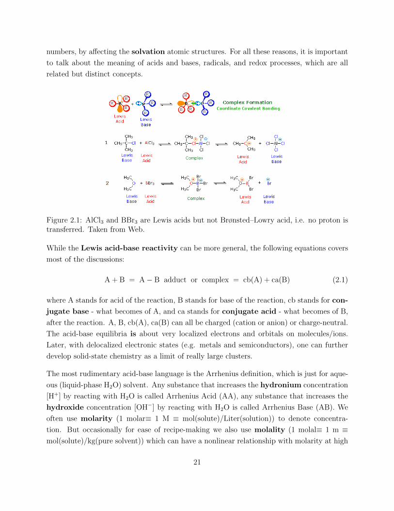
numbers, by affecting the solvation atomic structures. For all these reasons, it is important
to talk about the meaning of acids and bases, radicals, and redox processes, which are all
related but distinct concepts.
Figure 2.1: AlCl3 and BBr3 are Lewis acids but not Brønsted–Lowry acid, i.e. no proton istransferred. Taken from Web.
While the Lewis acid-base reactivity can be more general, the following equations covers
most of the discussions:
A + B = A− B adduct or complex = cb(A) + ca(B) (2.1)
where A stands for acid of the reaction, B stands for base of the reaction, cb stands for con-
jugate base - what becomes of A, and ca stands for conjugate acid - what becomes of B,
after the reaction. A, B, cb(A), ca(B) can all be charged (cation or anion) or charge-neutral.
The acid-base equilibria is about very localized electrons and orbitals on molecules/ions.
Later, with delocalized electronic states (e.g. metals and semiconductors), one can further
develop solid-state chemistry as a limit of really large clusters.
The most rudimentary acid-base language is the Arrhenius definition, which is just for aque-
ous (liquid-phase H2O) solvent. Any substance that increases the hydronium concentration
[H+] by reacting with H2O is called Arrhenius Acid (AA), any substance that increases the
hydroxide concentration [OH−] by reacting with H2O is called Arrhenius Base (AB). We
often use molarity (1 molar≡ 1 M ≡ mol(solute)/Liter(solution)) to denote concentra-
tion. But occasionally for ease of recipe-making we also use molality (1 molal≡ 1 m ≡mol(solute)/kg(pure solvent)) which can have a nonlinear relationship with molarity at high
21
concentrations. Since 1 kg(pure H2O solvent) corresponds to 1000/(2 × 1.008 + 15.999) =
55.5093 mol(H2O), assuming the addition of AA/AB and perhaps even some metal salts
does not change the volume (this is indeed a big if), then 1 M of [H+] (pH=0) roughly
corresponds to 1 H+ per 55 unsplit H2O molecules. Even if the proton grabs one H2O to
form H3O+ (the actual hydronium - this is also a Lewis adduct), and also has three water
molecules surrounding the H3O+ to form the solvation shell, there are still 51 free water
molecules left! So 1 M is not very high concentration yet, and one can certainly go to negative
pH≡ − log10([H+(aq)]/M) if one wants! But on the other hand, something like 10M should
be quite high concentration aqueous solution, since one may start to run out of relatively
free H2O solvent molecules. Also, the equilibrium constant Keq of the auto-ionization:
H2O(aq) = H+(aq) + OH−(aq) (2.2)
is a temperature dependent quantity
a[H+(aq)]a[OH−(aq)]
a[H2O(aq)]= Keq(T ) (2.3)
where a stands for activity - a proxy function of the chemical potential of the species in the
bracket - and in the dilute limit a for the solutes can be substituted for by the mole fraction.
So [H+(aq)] and [OH−(aq)] are constrained. AB would increase [OH−(aq)] and pH, while
AA would increase [H+(aq)] and decrease pH. However, [H+(aq)][OH−(aq)] ≈ 10−14M2 is
only approximately true near room temperature (indeed the concept of “room temperature”
varies from 300K=26.85 Celsius to 25 Celsius to 20 Celsius, and generally means “not very
well controlled experimental temperature” condition).
Brønsted-Lowry acid (BLA) and Brønsted-Lowry base (BLB) also talk about the proton H+
and is part of the “proton cult”, but not necessarily in liquid H2O solvent:
BLA + BLB = cb(BLA) + ca(BLB) (2.4)
where BLA donates a H+ to BLB. For example, acetic acid CH3COOH is a polar solvent,
and can dissolve oils. Methylamine CH3NH2 is a gas. The two can react like
CH3COOH(L) + CH3NH2(g) = CH3COO−(L) + CH3NH3+(L) (2.5)
where CH3COOH is the Brønsted-Lowry acid (proton donor), CH3COO+(L) solvated in the
liquid phase is the conjugate base; CH3NH2 is the Brønsted-Lowry base (proton acceptor),
22

and CH3NH3+(L) solvated in the liquid phase is the conjugate acid. The conjugate acid/base
terminology is because reactions like (2.5) are always reversible in principle, and those that
accept a gift can always give the gift back.
The fixation on proton in Arrhenius acid/base (aqueous, OH−) and Brønsted-Lowry acid/base
(not necessarily aqueous, not necessarily OH−) is justified because of the special “electron-
free” nature of H+ among all atoms on the periodic table. One can also say, there is only
LUMO(H+) which is just the 1s orbital, but there is no HOMO(H+) for the obvious reason
that H+ has no electrons at all. Therefore, H+ can only be Lewis acid, and a hard Lewis
acid since the LUMO is 1 Bohr radius = 0.529 AA in extent (see below). Anything that
offers LP to bond with H+ will be the Lewis base. One may argue that He,Ne,Ar,Kr,Xe,Rn
have no valence electrons to offer either, but KrF2, XeF6, XeO4, etc. make such absolute
noble gas claims a bit suspicious. Indeed the formation of KrF2, XeF6 suggests HOMO(Kr),
HOMO(Xe) can participate in the interaction with LUMO(F) (although LUMO(F) has a
radical situation, so the Lewis acid/base reactivity does not apply).
A proton is a ne’er-do-well, wondering adult male character, and is a true nucleus that
nucleophiles (i.e. HOMO-LP offering molecular fragments) like, because electron lone pair
(“children”) looks forward to be shared with another adult besides its original owner to
form a bond. The spatial extent and electronic polarizability of the said LP “children”
defines the hardness/softness of the Lewis base. Hard base has spatially small/tight LUMO
and low polarizability (“not impressionable”), for example F−, hydroxide OH− anions, and
ammonia NH3. All these satisfy the octet rules (no radicals), but the LP centered on F,
O, N are small because of low-Z. Soft base has spatially larger/diffuse LUMO and large
polarizability, for example iodide anion I− (because of high-Z), benzene C6H6 (because of
aromatic delocalization).
The same definition also for Lewis acids: Hard acid has LUMO that are small/tight in
spatial extent and not easy to polarize under electric field, for example H+, Li+, H3O+,
boron trifluoride BF3, and U4+. In the case of BF3, recall that boron element has 3 valence
electrons (electronic shell B=2.3), and these 3 valence electrons would be stripped pretty far
away from boron nucleus, and so the LUMO would see more the “bare B nuclide” and will
shrink in size, making it hard. In contrast, soft acid has LUMO that are large/diffuse in
spatial extent and easy to polarize under electric field, for example Ag+ (because of high-Z),
BH3 (because the electrons from the hydrogens are further screening the positive charge of
the “bare B nuclide” and thus push out the LUMO orbital size), and bulk metal M0 (the
LUMO of bulk metal is no different from its HOMO – both very large).
23
Borderline-hardness Lewis acids are Fe2+ (Fe=2.8.14.2), Co2+ (Co=2.8.15.2), Cs+, Pb2+
(Pb=2.8.18.32.18.4), that offer intermediate-sized LUMO. Borderline-hardness Lewis bases
are chloride Cl−, bromide Br−, nitrate NO3−, sulfate SO4
2− anions with HOMO-LP on Cl,
Br, N, S. The sizes of these HOMO-LP (“children under the care of single parent”) are
intermediate because these are quite a number of valence electrons, and also the screening
within polyanions is intermediate.
Ralph Pearson’s Hard-Soft Acid-Base (HSAB) theory (1963) says that “Hard Acid reacts
strongly with Hard Bases, and Soft Acid reacts strongly with Soft Bases”. Strong/weak
interaction (measured in eV or kJ/mol) is a different metric from hardness/softness, which
is about spatial extent of frontier orbitals. The HSAB theory has been widely verified in
chemistry.
http://li.mit.edu/A/Reference/Modeling/Papers/AcidBase/Lecture23HardSoftAcidBaseTheory.pdf
Here comes the electronic-structure story of chemistry, which addresses where the electrons
are now (the electronic configuration) and how they can be rearranged. Here are some
broad types of electronic transformations:
1. EA (electron affinity) versus IP (ionization potential), when an electron deciding to
join a cluster or leave a cluster, changing the total number of electrons this cluster
can call “its own”, which the essense of redox, valence, defect charge state, etc.
If the cluster is large enough to become a condensed phase, this gives rise to band
structure εn(k), electronic density of states (DOS) g(ε), the Fermi-Dirac distribution
0 < F (ε) < 1 at thermal equilibrium, the Fermi energy which is actually a chemical
potential EF ≡ µe ≡ −eU and is also related to the workfunction in surface science
and the equilibrium potential U that one reads out in a voltmeter in electrochemical
measurements. These are terminologies we will develop in detail later. This is also
related to the electropositive elements (like Li, Na, H) versus electronegative
elements (like F, Cl, O) on the electronegativity scale.
2. Lone pair (total spin 0, diamagnetic) versus radical (spin 1/2, paramagnetic). Since for
a given electronic spatial wavefunction (if localized, this will be called an orbital φ(x)),
an electron can occupy φ(x)| ↑〉 while another electron can occupy φ(x)| ↓〉. It turns
out that most often in chemistry, a doubly occupied φ(x) provide extra stabilization.
But there are plenty of examples of radicals also, for example, a lot of charge-neutral
isolated atoms can be considered radicals. See also for example the charge-neutral
hydroxyl radical (·OH), which is after taking one electron away from (i.e. oxidizing)
24
the three-LPs hydroxide anion (OH−). The charge-neutral ·OH is the second most
oxidative species in nature after fluorine, and can be generated by electrochemical
means to remove organic wastes in water [8]. So radicals can be associated with
EA/IP operations, but not always, for example the breakup of Cl2 molecule (with 6
LPs) into Cl2 = Cl· + ·Cl, each with 3 LPs and 1 radical, does not involve redox.
In the interaction of radiation with matter, plasma chemistry, etc., there is a lot of
radicalization also.
3. Promotion, hybridization: an isolated atom has spherical symmetry, and s-orbital
φl=0(x) = s(x) has lower energy than p-orbitals φl=1(x) = px(x), py(x), pz(x). Hy-
bridization means some linear combination of atomic orbitals (LCAO) into
h1(x) = s(x) + px(x) + py(x) + pz(x) (2.6)
h2(x) = s(x) + px(x)− py(x)− pz(x) (2.7)
h3(x) = s(x)− px(x) + py(x)− pz(x) (2.8)
h4(x) = s(x)− px(x)− py(x) + pz(x) (2.9)
These sp3 hybridized orbtials are higher-energy mixed states, and are thus called pro-
moted. For example, a carbon atom = 2.4 (1s22s22p2), when promoting its own 4
electrons to h1(x), h2(x), h3(x), h4(x) would have four radicals and quite high energy
(the promotion energy), but when forming CH4 would satisfy the octet rule for carbon
(and doublet rule for hydrogen), in a tetrahedral geometry. Resonance
4. Resonance, delocalization/localization:
5. Lone pair to bond transition, which is the essence of the Lewis acid/base concept.
In the Lewis perspective, we should focus on what happens to the electronic LP, in-
stead of on the proton, because the story of the electronic LP (who provided it, who
accepts it) is a main storyline of chemistry. A Lewis Acid (LA) is a cluster that will
increase/accept #LPs (note, not increasing #radicals, as most chemical reactions we
are familiar with do not involve radicals), because LA loves electronic LP (electrophile
before the reaction). A Lewis Base (LB) is a cluster that will decrease/donate #LPs,
because LB loves electron-barren proton or other LP-barren entities (at least in the
spatial direction of bonding), and thus is called nucleophile before the reaction. Lewis
base is most often also a BLB, but a Lewis acid (such as AlCl3, BBr3) does not have
to be a Brønsted–Lowry acid as it does not necessarily eject protons.
25
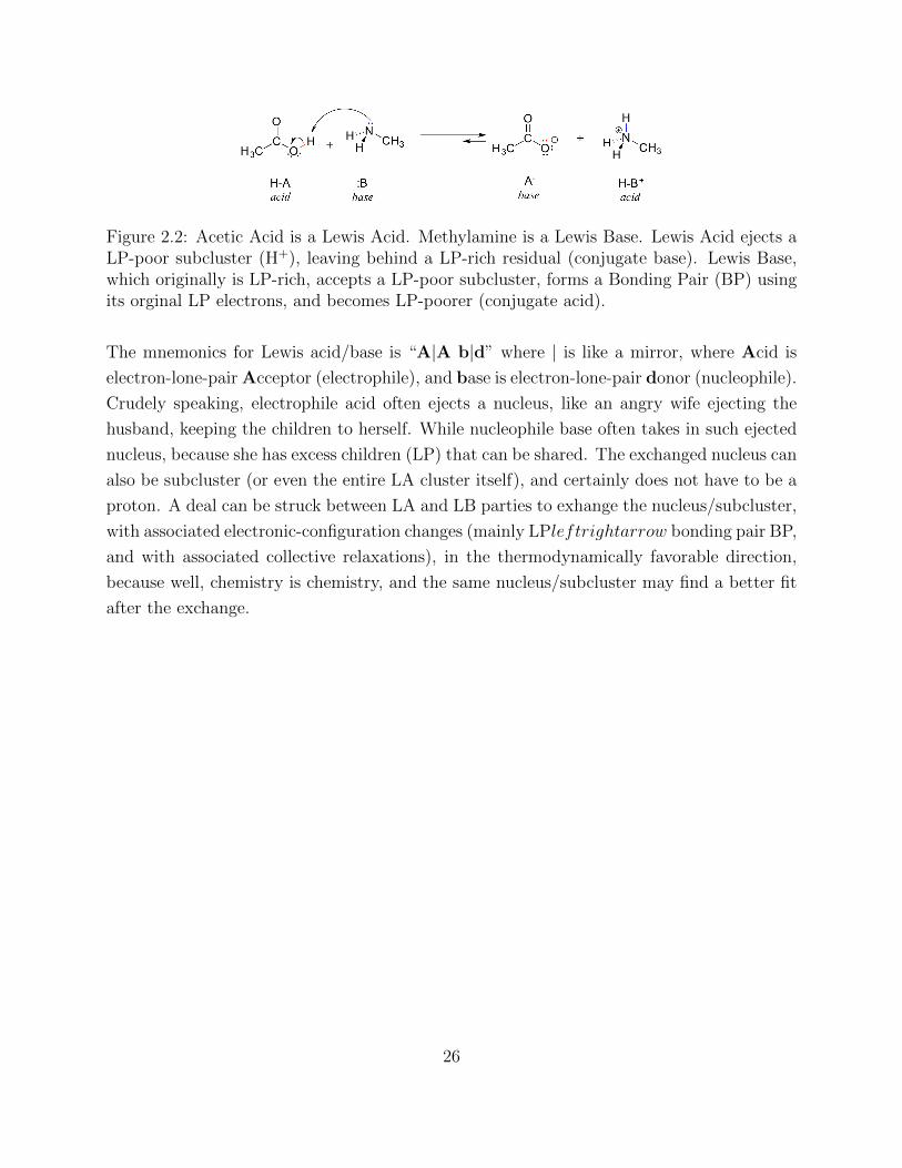
Figure 2.2: Acetic Acid is a Lewis Acid. Methylamine is a Lewis Base. Lewis Acid ejects aLP-poor subcluster (H+), leaving behind a LP-rich residual (conjugate base). Lewis Base,which originally is LP-rich, accepts a LP-poor subcluster, forms a Bonding Pair (BP) usingits orginal LP electrons, and becomes LP-poorer (conjugate acid).
The mnemonics for Lewis acid/base is “A|A b|d” where | is like a mirror, where Acid is
electron-lone-pair Acceptor (electrophile), and base is electron-lone-pair donor (nucleophile).
Crudely speaking, electrophile acid often ejects a nucleus, like an angry wife ejecting the
husband, keeping the children to herself. While nucleophile base often takes in such ejected
nucleus, because she has excess children (LP) that can be shared. The exchanged nucleus can
also be subcluster (or even the entire LA cluster itself), and certainly does not have to be a
proton. A deal can be struck between LA and LB parties to exhange the nucleus/subcluster,
with associated electronic-configuration changes (mainly LPleftrightarrow bonding pair BP,
and with associated collective relaxations), in the thermodynamically favorable direction,
because well, chemistry is chemistry, and the same nucleus/subcluster may find a better fit
after the exchange.
26
Chapter 3
Solvation Model and Debye–Huckel
Equation
At equilibrium, all the free agents are seeking maximum marginal happiness (or minimum
price). Given
pi = zieφ+ µi + kBT ln ai (3.1)
and in dilute solution, we have
pi ≈ zieφ+ µi + kBT ln ci/1M (3.2)
we see that if there is meso-scale φ(x) variation, we need to have
ci = c∞i e−zieφ/kBT . (3.3)
which is the same as distribution of O2 molecules on Earth surface despite mO2gh gravita-
tional potential energy.
But this would surely violate electroneutrality! (cation concentrations increase, while anion
concentrations decrease)
The total charge density therefore would vary as
ρfree(x) =∑i
ziec∞i e−zieφ/kBT , (3.4)
27
and the equation
∇2φ(x) = −∑i ziec
∞i e−zieφ(x)/kBT
ε(3.5)
where c∞i is the far-field concentration at φ = 0 (electrostatic potential reference) that must
also satisfy bulk charge neutrality.
(3.5) is called the Poisson-Boltzmann equation. It is a nonlinear PDE and generally requires
a numerical solver. But assuming
eφ(x) kBT (3.6)
we can linearize the equation, and get
∇2φ(x) =e2∑
i z2i c∞i
kBTεφ(x) (3.7)
The ionic strength is defined as
I ≡ 1
2
∑i
z2i c∞i (3.8)
Thus 0.1M MgCl2 would have
I =1
2(0.1× 4 + 0.2× 1) = 0.3M (3.9)
and we can define Debye length
λ ≡√kBTε
2Ie2=
3.04A√I
(3.10)
So, for 0.1M MgCl2 in water, we have λ = 5.55A.
Truly, 5.55A is very short and it is not clear that the continuum approximation would work
well. However, there are more extreme examples than this, which is a metal! A metal can be
thought as a high density soup of electrons and holes. The carrier concentration in copper is
1e/11.81E-30 = 141 M, and the equivalent I = 70.3M (partly thanks to the atomic density
of copper). Thus, λ = 0.36A. Because λ a0 the lattice constant, this is just saying that
electronic screening is so strong that it probably does not even make sense to talk
about ions in good metals like Cu. Now actually since pe include quantum effects also,
one should really use the Thomas–Fermi screening model instead of Debye–Huckel screening
that uses Boltzmann statistics, but the basic conclusion holds, which is that a metal is
too good an “electrolyte” (for electrons, not ions) to even talk about ionization. Now in a
28
semiconductor, where the free carrier density is much lower, it still makes sense to talk about
ionization, e.g. a Boron dopant capturing a valence band edge electron and becomes an
anion B−Si (with paired electron) embedded in Silicon lattice, while leaving a free hole [h] in
Bloch state inside the silicon.
So
∇2φ(x) =φ(x)
λ2, x 6= 0 (3.11)
can be solved for the parallel-plate and point-charge situations also.
First imagine a flat electrode at x = 0, and electrolyte in x > 0:
d2φ
dx2=
φ(x)
λ2, x = (0,+∞) (3.12)
the stable solution is obviously
φ(x) = φ0e−x/λ, E(x) =
φ0
λφ0e
−x/λ, (3.13)
with areal charge densityρ
A= ε∇ · E =
εφ0
λ(3.14)
at x = 0, and volumetric screening charge density
ρfree = −ε∇2φ = −εφ0
λ2e−x/λ (3.15)
It is clear that this is effectively a double-layer capacitor, with equal and opposite charge
− ρA
at the mean distance
d = λ. (3.16)
Thus, the effective capacitance would be
C
A=
ε
d=
ε
λ=
√2Iεe2
kBT(3.17)
that fully screens out whatever surface charge density we put into the electrode.
In the point-charge case, we have
∇2φ(x) = −zeδ(x)
ε+φ(x)
λ2, x 6= 0 (3.18)
29
φ(x) =zee−r/λ
4πεr(3.19)
since
∇2φ = r−2∂r(r2∂rφ) =
ze
4πεr−2∂r(r
2(−r−2e−r/λ − r−1e−r/λ/λ))
= − ze
4πεr−2∂r(e
−r/λ + re−r/λ/λ)
= − ze
4πεr−2(−e−r/λ/λ+ e−r/λ/λ− re−r/λ/λ2)
=ze
4πεr−1e−r/λ/λ2
=φ
λ2. (3.20)
However, just like in the solvation-shell theory, in reality there is excluded volume that
counter-ions cannot get into. Imagine we have a cation z+e at r = 0, and the closest that
the anion can get to is rcut = r+ + r−, where r+, r− are the cation and anion ionic radius, so
rcut is a hard core. In this case, the solution needs to be modified, as,
φ(r) =
A−z+e4πεrcut
+ z+e4πεr
, r < rcut
A exp((rcut−r)/λ)4πεr
, r > rcut
(3.21)
where the total screening charge must still be −z+e:
−z+e =∫ ∞rcut
4πr2dr(−ε)A exp((rcut − r)/λ)
4πεrλ2= −
∫ ∞rcut/λ
Ardr exp(rcut/λ− r)
= −A(rcut/λ+ 1), (3.22)
and so
A =z+e
rcut/λ+ 1(3.23)
so we get the excess stablization electrostatic potential due to screening charge is
A− z+e
4πεrcut
= − z+e
4πεrcut
(1− 1
rcut/λ+ 1) = − z+e
4πεrcut
rcut
rcut + λ= −z+e
4πε
1
rcut + λ, (3.24)
which is an eminently sensible result after such laborious derivations.
But remember this stabilization energy is equally shared between the central cation and
surrounding anions, so there is a factor of 1/2, and the excess stablization energy can be
30
identified as
kBT ln γ+ = −z2
+e2
8πε(rcut + λ)(3.25)
We also have, complimentarily for the anion,
kBT ln γ− = −z2−e
2
8πε(rcut + λ)(3.26)
Generally speaking suppose the binary salt formula looks like Z+ν+Z−ν− , we have
ν+z+ + ν−z− = 0 (3.27)
(note that ν+, ν− > 0, while z− < 0) and we can define
ν ≡ ν+ + ν− (3.28)
with mean activity a± defined as
νkBT ln a± ≡ ν+kBT ln a+ + ν−kBT ln a− (3.29)
aν± ≡ aν++ a
ν−− . (3.30)
Given c M of Z+ν+Z−ν− , we will have
c+ = ν+c, c− = ν−c (3.31)
and so
a+ = γ+ν+c, a− = γ−ν−c (3.32)
so
aν± = (γ+ν+c)ν+(γ−ν−c)
ν− = (γ+ν+)ν+(γ−ν−)ν−Xν (3.33)
so we can also define mean activity coefficient
γν± ≡ γν++ γ
ν−− , (3.34)
to get
aν± = (γ±c)νν
ν++ ν
ν−− . (3.35)
31

Finally, given the Debye–Huckel result, we will have
ln γ± =ν+ ln γ+ + ν− ln γ−
ν= −
ν+z2+e
2 + ν−z2−e
2
8πεkBT (rcut + λ)ν= −ν−z−z+e
2 + ν+z+z−e2
8πεkBT (rcut + λ)ν
= − z+z−e2
8πεkBT (rcut + λ)(3.36)
where λ ∝ I−1/2.
The Debye–Huckel model works quite well for binary electrolyte in the dilute limit.
32
Chapter 4
Electrode Kinetics
In Chap. 1 we have shown the basic thermodynamic relation between a free electron in
the metal (or semiconductor) electrode of µe ≡ EFermi ≡ −eU ,
f(ε) =1
1 + eε−µekBT
=1
1 + eε+eUkBT
(4.1)
and ion/atom pair ∆G(T, P ) + kBT lnQ. The gist is: the electron (“child”) abandoned
behind in the metal is the outcome of an ionization reaction of the atom (living in some
phase) and jumping into perhaps another phase as an ion, resulting often in the ion in
phase and the electron child in another phase (unless auto-ionization like dopant in silicon).
This involves a change in the chemical identity of the atom. Such change in chemical
identity, specifically the chemical valence of some elements, causes a Faradaic current.
More generally, we can replace the word atom by any molecular fragment.
The definition of U thus must be covariant with the definition of ∆G(T, P ) for the
ion/atom pair. If U = 0 is taken to be the vaccuum (4.44 eV above SHE with aqueous
electrolyte), then the definition of ∆G(T, P ) ≡ price(ion)−price(atom), when talking about
price(ion), need to talk about the true electrochemical price of the ion living in the liquid, and
thus would have to include the electrostatic potential average of the liquid. (price(atom) does
not care, but price(electron) does care about what its environmental electrostatic potential
average is).
If U = 0 is taken to be the average electrostatic potential of the liquid phase, then ∆G(T, P )
just contains the chemical part of the ion’s price in standard condition. This is a nice sim-
33
plification conceptually, because then the entire ∆G(T, P ) + kBT lnQ is chemical (local)
and free of electrostatics. Then, under this definition, the environmental electrostatic po-
tential average of the metal electrode with respect to the liquid it is in contact with need to
be added to the price(electron) (but the quantum and the thermal are also there inside the
price(electron), which are also local). This is the most “physical” definition, because then
the equilibriating process (when the price does not match) by a small change in the EDL
can shift this environmental electrostatic potential difference, without significant change in
the bulk composition. This occurs because 1ML of Mg dissolving can cause 36.19×2 =72.38
Volt shift, if all the electrons left behind stays on the metal surface (which they are likely to
do). 0.01ML of anything dissolving is not observable at bulk scale, and thus the equilibra-
tion process can establish the equilibrium (and the open-circuit potential) with “barely any
visible” change.
If U = 0 is taken to be the SHE, then the electron energy ε is in reference to the Fermi
level of the bubbling Pt (but could be any other metal, because the ion/atom pair we are
actually talking about is H+/H2
2, not Pt - Pt is just a host, although a kinetically facile
one) in contact with the same liquid electrolyte, and ∆G(T, P ) would actually have the
µH+ −µH subtracted off, for every electron left behind that we are counting. So you can say
the ∆G(T, P ) in this metric to be not “pure”. But measurement wise, it is the most easy
thing to do.
4.1 Butler-Volmer and Exchange Current Density
Once the thermodynamic picture is clear, the kinetics is easy. Some atoms strips the electrons
and jump into ocean (anodic), and some ions climb out of the electrolyte onto the metal and
recombine with the electron (cathodic). The total curent density on electrode surface can
be net anodic (by convention, this give positive i [Amp/m2] – in other words, if the current
vector (which is oppostite to the electron flow vector) is pointing into the electrode), or
net cathodic (by convention, this gives negative i – in other words, if the the current vector
(which is oppostite to the electron flow vector) is pointing out of the electrode). Consider
the following paradigm:
R = O + e− (4.2)
where in this example, both R and O are living inside the liquid electrolyte. (this does not
have to be case, but we are using this as pedagogical example).
34
The actual microscopic ionization process could be very complicated. To get close enough
to the metal electrode, R may need to break up its solvation shell, to get onto the inner
Helmholtz plane (IHP) (see Fig. 3.2 of [4]) and be directly adsorbed. Such ad-ion configura-
tion could be labelled Rs where superscript s is a surface site. The same for Os, so generally
the process could be R → Rs → Os → O. It turns out that anions, because of weaker
interaction with its solvation shell (larger), are preferentially found in IHP than cations.
Or, perhaps electron transfer could happen when R is in the outer Helmholtz plane (OHP),
which is the distance of closest approach for a solvated ion that keeps its solvation number
intact.
For simplicity, let us take dilute liquid solution with known concentrations cR, cO near
the surface, and assuming the redox is happening for OHP situation, we have
ia = kacRe−Qa/kBT , ic = kccOe
−Qc/kBT (4.3)
where Qa ≡ E∗ − ER and Qc ≡ E∗ − EO+e are the microscopic energy barriers. Note
that EO+e contains the energy of both O and e−, separated by the EDL, and thus EO+e
will depend on U . If we take the liquid environmental electrostatic background to be zero,
then ER, being living fully in the liquid phase, does not depend on U . The saddle point
configuration in between, as the nuclide crosses the EDL, will have energy E∗ that depends
partially on U , but not as much as EO+e. So we can say that
∂ER
∂U= 0,
∂E∗
∂U= −e(1− β),
∂EO+e
∂U= −e, (4.4)
where 0 < β < 1 is called the symmetry factor.
At equilibrium potential U eq (for the known and fixed cR, cO), we have zero net current, so
kacRe−Qeq
a /kBT = kccOe−Qeq
c /kBT (4.5)
from our micro-kinetics model, or
Qeqa = Qeq
c − kBT lnkccO
kacR
. (4.6)
and so
E∗ − ER = E∗ − EO+e − kBT lnkccO
kacR
. (4.7)
The activated state cancel from both sides, and we see that at electronic equilibrium, we
35
have
0 = ER − EO+e − kBT lnkccO
kacR
, (4.8)
This is equivalent to our stated thermodynamic principle for dilute solution
0 = ∆G = ER − EO+e − kBT lnkccO
kacR
, (4.9)
if we recognize that the Gibbs free energy driving force ∆G contains configurational entropy
contributions kBT ln cO − kBT ln cR, similar to our stated thermodynamic driving force of
∆G = pR − (pO − eU) (4.10)
for net-anodic reaction. This is called detailed balance principle, or thermodynamics-
kinetics equivalence. The kinetic constants kBT ln kc, kBT ln ka, can be absorbed into ER,
EO+e as some kind of “vibrational free energy”, by normalizing with the constant prefactor
k0cref , in other words if we identify
pR ≡ ER + kBT ln kacR/k0cref , pO ≡ EO + kBT ln kccO/k0cref , Ee ≡ −eU (4.11)
so the prices include vibrational and configuratinal entropy terms, and by definition of U eq,
we have
0 = ∆G = pR − (pO − eU eq), (4.12)
that we have asserted in Chapter 1 without detailing.
We can therefore define the exchange current as
i0 = kacRe−Qeq
a /kBT = k0crefe−(E∗−pR)/kBT , (4.13)
i0 = kccOe−Qeq
c /kBT = k0crefe−(E∗−pO+eUeq)/kBT (4.14)
Note that E∗ above is right at U = U eq for the given cR, cO.
For U 6= U eq for the given cR, cO, there will be
η ≡ U − U eq, (4.15)
which is defined as surface polarization overpotential, and so
ia = i0ee(1−β)η/kBT , ic = i0e
e(−β)η/kBT (4.16)
36
so we derived the famous Butler–Volmer equation
i = i0[ee(1−β)η/kBT − e−eβη/kBT ] (4.17)
for electronic (voltage) out-of-equilibrium situations.
It is important to recognize that i0 is defined at U = U eq(cR, cO) and thus depends on both
cR and cO. For example, even though (4.13) appears to depend on cR only on first look,
through the
∆E∗ = −e(1− β)∆U eq = (1− β)∆kBT lncR
cO
(4.18)
dependence, one ends up having
i0 ∝ c1−βO cβR (4.19)
This turns out to be important in discussing polarization voltage partition between long-
range transport and short-range charge-transfer reaction in mass-transport limited corrosion
(page 386 in [4]).
For multi-electron transfer reactions, such as
R = O + ne− (4.20)
we will generally have
i = i0[eeαaη/kBT − e−eαcη/kBT ] (4.21)
with the anodic transfer coefficient αa and cathodic transfer coefficient αc:
αa + αc = n, αa ≡ n(1− β), αc ≡ nβ (4.22)
and the exchange current density would scale as
i0 ∝ cαaO c
αcR . (4.23)
Note that the above is not cαaR c
αcO that one might be confused about!
37
4.2 Tafel Approximation
There are three regimes in (4.21): exponential, linear, and somewhere in between. The
exponential regime occurs when eαη kBT , where one can ignore one of the two terms,
and get
log10 |i| ≈ log10 i0 +eα|η|
2.3026kBT(4.24)
(4.24) is called the Tafel Approximation. Since 2.3026kBT = 59.16 meV, this means if
α = 0.5, every 118 mV increase in surface overpotential would cause 10× the current density.
This approximation is generally only valid when |η| 100mV. This calls for semi-log plot,
where the voltage is linear, but the current is plotted in log10-scale.
When |η| 10mV, we can also approximate (4.21) as
i = i0neη
kBT, (4.25)
this calls for linear-linear plot, but in linear-log plot would appear as a deep cusp at η = 0
or U = U eq, since log is unbounded in the negative value side.
4.3 Exchange current density and limiting curent den-
sity
Butler–Volmer is very “near-sighted” and describes electron transfer across nm distance,
and associated chemical indentiy change. The fact that η is defined based on local chemistry
(at so-called x=0)
38
Chapter 5
Long-range Mass Transport
Electrode kinetics, aka, charge-transfer (CT) reaction at phase boundaries, is very short
ranged, as electron can only tunnel a short distance. After some reactions have happened,
the products need to be transported away, and the reactants are exhausted and need to be
resupplied, otherwise U eq would shift and the net reaction would stop. How the reactants
are resupplied and products transported away is the topic of this chapter.
In a fluid electrolyte, ion/molecule would generally have flux
Ji = ci(vi + vCM) (5.1)
where vCM is center-of-mass translation of the fluid, and vi is the average velocity of species
i with respect to the center-of-mass frame. Thus, by definition
∑i
micivi = 0. (5.2)
Note that ci has unit #/m3, Ji has unit #/m2/s.
Solving for vCM (such as by solving Navier-Stokes equation with knowledge of viscosity) is
the business of fluid mechanics,
ρ
(∂tvCM
∂t+ vCM · ∇vCM
)= ρg −∇p+ η∇2vCM (5.3)
39
while modeling vi requires chemical solution thermodynamics. We generally model
vi = Mi(−∇pi) (5.4)
note that Mi has the unit m/s/N, and
pi = zieφ+ µi + kBT ln ai (5.5)
is the electrochemical potential, and so in the dilute solution limit, there is
pi = zieφ+ µi + kBT ln ci/1M (5.6)
and
−∇pi = −zie∇φ− kBT∇cici
(5.7)
and so
Ji = −Micizie∇φ−MikBT∇ci + civCM. (5.8)
The first term is called migration (or drift), which is driven by the electrostatic part of the
price. The second term is called diffusion, where we identify
Di = MikBT (5.9)
as the Einstein relation, and the third term is called convective term.
Without chemical reaction,
∂tci = −∇ · Ji (5.10)
and so the RHS consists of
∇ · (Micizie∇φ) +MikBT∇2ci = Mizie∇ · (ci∇φ) +Di∇2ci (5.11)
and
−∇ · civCM = −ci∇ · vCM − vCM · ∇ci. (5.12)
For incompressible fluid, ∇ · vCM ≈ 0, and so the conservation equation can be written as
∂tci + vCM · ∇ci = Mizie∇ · (ci∇φ) +Di∇2ci. (5.13)
The LHS is also called “Material derivative”.
40
The charge flux is
i =∑i
zieJi =∑i
−ciMizie(zie∇φ+ kBT∇ci) + vCM
∑i
zieci (5.14)
Away from EDL, we can use bulk electroneutrality
ρtotal =∑i
zieci = 0 (5.15)
to eliminate the convective contribution. Also, when there is no concentration gradient
(homogeneous liquid), we will have
i = κ(−∇φ) (5.16)
where the electrical conductivity is
κ =∑i
ciMiz2i e
2 (5.17)
The unit of κ is
1/m3 ×m/s/N× C2 = C2/s/m/J = C/s/V = C/s/m/V = (Amp/m2)/(V/m) (5.18)
Since
Ohm ≡ V/Amp, Siemen ≡ Amp/V (5.19)
The unit of κ is also Siemen/m, or 1/Ohm/m. We use the symbol κ instead of σ for metal and
semiconductors to distinguish between ionic conduction of charge, and electronic conduction
of charge.
One can define the transference number
ti ≡ciMiz
2i e
2∑k ckMkz2
ke2
(5.20)
and in mixed ionic-electronic conductor (MIEC), k can include the electron/hole as well.
In the treatment above, we have ignored so-called Onsager off-diagonal coupling, where force
on species k, can induce motion and flux of species k′. A case in point is undissociated H2O.
According to (5.20) its transference number is zero. In other words, under electric field,
neutral water (or other charge-neutral molecules) would not be transported. But in fact,
41
because of hydration number (aka solvation number), H2O can be strongly bound to some
ions, and these ions when moving under electric field would drag the water with it. This
effect is especially true in hydrogen PEM fuel cells, where in addition to the new water
formed on the ORR electrode, the proton flux also brings additional water, so the cathode
tends to be flooded by excess water, while the anode tends to be dry, so constant water
management is needed (see page 208, [4]).
5.1 Binary-Salt Liquid Electrolyte
Now consider a salt Z+ν+Z−ν− with
z+ν+ + z−ν− = 0 (5.21)
and we can define salt concentration as
c ≡ c+
ν+
=c−ν−
(5.22)
Plugging into (5.13), since all terms are linear in c, we get
∂tc+ vCM · ∇c = M+z+e∇ · (c∇φ) +D+∇2c, (5.23)
∂tc+ vCM · ∇c = M−z−e∇ · (c∇φ) +D−∇2c, (5.24)
and we get
(M+z+ −M−z−)e∇ · (c∇φ) + (D+ −D−)∇2c = 0. (5.25)
The above is actually the condition to maintain (5.22) absolutely true, so it is an equality
to the degree that (5.22) is absolutely true (ie. away from phase boundary).
So in the bulk of the fluid, we can multiply M+z+ on the second equation and substract off
M−z− multiplying on the first equation:
(M+z+ −M−z−)(∂tc+ vCM · ∇c) = (M+z+D− −M−z−D+)∇2c, (5.26)
and get
∂tc+ vCM · ∇c = D∇2c, (5.27)
42
where the equivalent diffusion coefficient is
D =M+z+D− −M−z−D+
M+z+ −M−z−=
(z+ − z−)D+D−z+D+ − z−D−
. (5.28)
So even though (5.27) looks like a diffusion equation for the salt concentration, it actually
contains electric field and migration effects.
From the discussion on liquid junction potential, we know that when
M+ 6= M− (5.29)
a salt concentration gradient will slightly disturb bulk electroneutrality, and build up ∇φ,
a possibilty which is expressed in (5.25) also. So it seems rigorous bulk electroneutrality
cannot be true. Yet, derivations from (5.22) to (??) are used as bible everywhere, so it must
be a good approximation. So it means there must be a small dimensionless parameter
somewhere. How small is this small parameter?
In Section 1.1, the procedure was fixing ρ0, while extending the system size L and volume
L3, which led to the explosion as L → ∞. However, other types of taking limits could
also be considered. For example, keeping ∆φ to be a fixed value, while taking large L. In
this procedure, the system energy per volume does not explode. This is because the system
areal capacitance ε/d ∝ ε/L, so the areal charge density is actually decreasing as 1/L, and
multiplying with a finite ∆φ does not lead to any problem. This is the situation with the
liquid-junction potential. The amount of ρ0 is scaling with the salt-diffusional zone width L
as 1/L or faster. In Section 1.2, we have seen that two monolayers of charge e/5A2
separated
by 10 nm deionized water gap still gives 46 Volt. Thus a 1-Volt scale ∆φ spread over distance
L means an areal charge density e/5A2
4610nmL
= 1ML/(L/2A).
This is the samll parameter we are looking for. Given that L is macroscopic, like mm, we
get 1ML of charge spread over 106 “layers” of liquid. Thus, the degree of charge imbalance
is only 10−6, much smaller than the most c we are covering. (Indeed, 10−6 M is often the
smallest value one cares about in Pourbaix diagrams to be considered “present”). So one
can say, the error one makes in (??) is on the order of 10−6.
43
5.2 Electrorefinning Example
Now consider a pedagogical example of electrorefinning of copper in 1D, where at x = 0 one
has the anodic dissolution:
Cu(FCC99%pure) = Cu2+ + 2e−(Ua) (5.30)
and on the cathode at x = L, there is cathodic deposition:
Cu2+ + 2e−(Uc) = Cu(FCC99.99%pure) (5.31)
Based on the anode and cathode purity, and aCu2+ at x = 0 and x = L, there are two OCVs:
U eqa =
∆µ + kBT lnQa
2e, Qa ≈
cCu2+(x = 0)
aCu(FCC99%pure)
(5.32)
U eqc =
∆µ + kBT lnQc
2eQc ≈
cCu2+(x = L)
aCu(FCC99.99%pure)
(5.33)
and two over-potentials
ηa = Ua − U eqa > 0, ηc = Uc − U eq
c < 0, (5.34)
with
Ia = i0(x = 0)Aa[ee(1−β)ηa/kBT − e−eβηa/kBT ] (5.35)
and
Ic = −Ia = i0(x = L)Ac[ee(1−β)ηc/kBT − e−eβηc/kBT ] (5.36)
where Aa, Ac are the true surface areas. There is a power source U ext
U ≡ Ua − Uc = U eqa − U eq
c + ηa − ηc (5.37)
driving this ia current in the external circuit, that should be rated as
U ext − IaRext = U eq
a − U eqc + ηa − ηc (5.38)
where Rext is the external electronic resistance. We note that
U eqa − U eq
c =kBT
2elncCu2+(x = 0)aCu(FCC99.99%pure)
cCu2+(x = L)aCu(FCC99%pure)
, (5.39)
44
so the energy balance can be written as
U ext =kBT
2elnaCu(FCC99.99%pure)
aCu(FCC99%pure)
+kBT
2elncCu2+(x = 0)
cCu2+(x = L)+ IaR
ext + ηa − ηc. (5.40)
The first term is the OCV voltage, when there is no external current in the outer circuit and
no ion transport inside. The second term is the “ionic IR” drop, which can be merged with
the external circuit electronic IR drop to give the total IR drop:
RΩ = Rext +Rint, (5.41)
where
Rint ≡ kBT
2eIa
lncCu2+(x = 0)
cCu2+(x = L), (5.42)
and then ηa > 0, ηc < 0 drives the local electrodic processes.
The way we can think about kBT2e
ln cCu2+(x) as a potential is that suppose we use FCC 99%
pure as a zero-current probe electrode, then
Uprobe(x) ≡∆µ + kBT ln
cCu2+ (x)
aCu(FCC99%pure)
2e(5.43)
would have been the read-out at that liquid spot 0 < x < L. We would have
Uprobe(x→ 0) = U eqa , Uprobe(x) = U eq
a +kBT ln
cCu2+ (x)
cCu2+ (x=0)
2e(5.44)
Uprobe(x→ L) = U eqc +
kBT
2elnaCu(FCC99.99%pure)
aCu(FCC99%pure)
. (5.45)
So about the transport boundary conditions, we note that both electrodes are blocking to
anions, and so
J−(x = 0) = J−(x = L) = 0 (5.46)
Furthermore, if we assume no convection, then
−M−c−z−e∇φ−M−kBT∇c− = 0 (5.47)
45
on both borders. This often means that this is also true in the interior, so
dφ
dx= − kBT
c−z−e
dc−dx
(5.48)
and since
J+ = −M+c+z+edφ
dx−M+kBT
dc+
dx(5.49)
we get
J+ = −M+c+z+kBT
c−z−
dc−dx−M+kBT
dc+
dx(5.50)
Given that
c+z+ ≈ c−z− (5.51)
J+ = −M+kBT (dc−dx
+dc+
dx) = −M+kBT (ν+ + ν−)
dc
dx(5.52)
But we have
D =(z+ − z−)D+D−z+D+ − z−D−
. (5.53)
and
t− ≡c−M−z
2−
c+M+z2+ + c−M−z2
−= − c+M−z+z−
c+M+z2+ − c+M−z+z−
= − D−z−D+z+ −D−z−
(5.54)
soD
t−=
z+ − z−−z−
D+ = (1− z+
z−)D+ = (1 +
ν−ν+
)D+ (5.55)
therefore we have a simplified form:
J+ = −ν+D
t−
dc
dx= −ν+
D
1− t+dc
dx(5.56)
where the physics of −D dcdx
is the salt flux, and −ν+Ddcdx
is the associated cation flux with the
salt concentration diffusion equation (5.27). However, the actual J+ flux is bigger than that
by a factor of 1/(1 − t+). This is because the anode and cathode are both non-blocking to
z+, and so one can build up a current even without concentration gradient. Vice versa, even
if there is a finite salt concentration gradient, and a concentration-gradient driven −ν−D dcdx
term, the total J− can be zero, because of a countering electric field.
The point is that even with vCM = 0, there can be three kinds of processes simultaneously
going on within a binary electrolyte:
46
1. Neutral salt diffusion as represented by ∂tc = D∇2c. The wavelength of c(x, t), is say,
on the order of L, that can be varying on the order of L(t) ∝ (Dt)1/2 for transient
problems, or it may reach steady-state after L(t) has hit the boundaries of the system.
But generally speaking, L(t) is on the order of µm or above.
2. Establishment of liquid junction potential ∇φ. The derivations from (5.23),(5.24)
show that in transient conditions, if M+ 6= M− and there is an evolving concentration
gradient; or in steady-state conditions with blocking electrode for ion, like (5.47),
then we will build up ∇φ. The details actually does not matter for the ∂tc = D∇2c
neutral salt diffusion problem, because the “salt polarization” (center-of-mass of cations
devitating from the center-of-mass of anions) which gives∇φ, is on the order of ∆φ/IL,
and this distance is so minuscule:
d ∝ (∆φ)ε
IeL∼ 1Volt× ε
1M× 1µm× e= 7.194547702197474E − 12m (5.57)
and so
d L(t) (5.58)
by at least 6 orders of magnitude, such that such offset
c+(x, t) = ν+c(x− d/2, t), c−(x, t) = ν−c(x+ d/2, t) (5.59)
would cause very weak breaking of bulk electroneutrality, that it does not matter for
∂tc = D∇2c. Nontheless, such “salt polarization” orthogonal to the salt-diffusion is
a higher-order physical process that can be (and is in fact likely) going on inside the
system.
3. At steady-state, the boundary condition obviously matters. The fact that we have
J− = 0 in this 1D problem, while J+ is boosted by 1/(1− t+) is caused by the ∇φ, or
we can say, ∇φ evolved to be this way to satisfy the anion-stagant, cation-moving BC.
5.3 1D Cation Transport without Convection
Section 5.2 for electrorefinning is applicable to problem like Lithium-ion Batteries, which is
blocking to anions but non-blocking to the working cation. Consider ν+ = 1, z+ = 1, ν− = 1,
z− = −1, κ = 1.3 Siemens/m, t+ = 0.4, and salt concentration 0.8 M. The 1D gap distance
47
is L = 200E − 6 m.
We have
c+z2+e
2M+ = 1.3×0.4, c+ = ν+c = 0.8×AV O/1E−3 → M+ = 4.2047644E+10m/s/N
(5.60)
c−z2−e
2M− = 1.3×0.6, c− = ν−c = 0.8×AV O/1E−3 → M− = 6.3071466E+10m/s/N
(5.61)
The salt diffusivity is then
D =2D+D−D+ +D−
= 2.077E − 10m2/s (5.62)
So the timescale for two electrodes to communicate with each other through diffusion in
liquid electrolyte is
L2/D = 192.58s (5.63)
This is quite a bit faster than the typical battery charging and discharging timescale (graphite-
anode batteries are typically limited at 2C, or 30min charging time).
We see that at steady state, the Li+ cation flux is
J+ = −ν+D
1− t+dc
dx(5.64)
This means that the steady-state solution must be linear profile. And since the total cation
number is conserved in the liquid electrolyte, we have c(x = 100E−6) = 0.8×AV O/1E−3,
and it looks like a symmetric seesaw.
The limiting current is the maximum current that can be supported by long-range transport
in the system, and therefore
ilim = z+emax J+ = e× D
0.6max
dc
dx= e× D
0.6
1.6× AV O/1E − 3− 0
L= 267.21Amp/m2 = 26.7mA/cm2.
(5.65)
Say we are charging, and x = 0 is the graphite with cathodic current (Li+ cation coming
toward it in the electrolyte), and x = L is the LCO positive electrode with anodic current
(Li+ cation leaving it in the electrolyte)
When c(x = 0)→ 0, the electrodic exchange current would be so low that the overpotential
48
ηc would need to be so negative, that one could have Li-metal precipitation on the electroide.
Also, if c(x = L) is too high, it may exceed the solubility limit of the salt (say it is LiFSI)
in the electrolyte, that solid salt could precipitate out. Both are catastrphes that one need
to avoid, so ilim is the physical upper bound, and may not be attainable.
So even if there is no electrodic limitation on either anode or cathode side, the maximum
charging time to charge a standard 3mAh/cm2 electrode would take
3mAh/cm2/26.7mA/cm2 = 0.112h, (5.66)
or in other words, limited to 9 C. To increase this rate, one needs to reduce L. Current
separators are as thin as 10 micron, raising the rate capability from limiting current to 180
C, but there will be electrodic limitation as well as we will see next.
At the limiting current, we will have, from (5.48),
dφ
dx= − kBT
c−z−e
dc−dx
(5.67)
so there is actually a problem as c→ 0, since we will have divergence in dφdx
. Indeed, we can
see that
∆φ = −∆(kBT ln c−)
z−e(5.68)
so it is not possible for c− to be actually 0. Thus the (5.65) transport-limited current is
only an approximation, and a slight overestimate.
Q: Suppose from an open-circuit condition, the external circuit suddenly imposes
electronic current ilim/2 = 13.36mA/cm2 at t = 0, what would be the voltage drop
inside the electrolyte?
A: This is a tricky question. The areal capacitance between the two electrodes is very low:
C/A =ε
L= 3.470841622617600e− 06Farad/m2 = 3.470841622617600e− 10Farad/cm2
(5.69)
thus, within C/A/(ilim/2) = 2.597935346270658e − 08 s, if there is no ionic currents, the
voltage would have risen by 1 Volt across the two electrodes. Within such short time, there
is no time for the homogeneous salt concentration to redistribute (since we see the diffusional
49
time is few hundred seconds). Thus, an ionic charge current will be induced as
iionic = ∆φ× 1.3S/m/200E − 6 (5.70)
and to stop the meteoric rise in φ, there needs to be
iionic = ilim/2 (5.71)
and so ∆φ = 133.6× 200E − 6/1.3 = 0.02055V inside the electrolyte.
Note that this ∆φ is only inside the electrolyte, and not between the two metallic electrodes.
Between the metallic electrode and the liquid electrolyte this is EDL, and when ∆φ is small
the electrodic current is small (small leakage), and most of the electronic current in the metal
and ionic current in the electrolyte just accumulate across the EDL, and this will build up
the ∆interfaceφ which contriutes to η, so such interface, even if not ideally polarizable, is quite
polarizable. But as η gets larger and larger, the leakage current (Faradaic current) gets
exponentially larger, and eventually η stops growing. This will be turned in the effective
circuit model in the next Chapter.
But regardless of the partition inside the Angstrom-level EDL into Faradaic leakage current
or double-layer charging current, it is immaterial to the voltage drop inside the few-hundred-
micron-thick liquid electrolyte, which is 20.55 mV, due to separation of length and timescales.
It is only after a few hundred seconds that this will change due to concentration polarization.
Q: What is the steady-state voltage drop inside the liquid electrolyte?
A: For ilim/2, we have half of the “limiting slope”
c(x = 0) = 0.4M, c(x = L) = 1.2M (5.72)
at steady-state, and so
∆φ = −∆(kBT ln c−)
z−e= kBT (ln 3)/e = 28.226mV. (5.73)
In charging, the electrostatic background inside the liquid electrolyte must be such that it
repels the anions from coming toward the x = 0 graphite electrode. Thus φ(x→ 0) must be
smaller than φ(x→ L). The sign does work out.
Page 75 of [4] seems to get the sign wrong. It said “Once sufficient time elapses, a
50
concentration gradient will develop and the modified form of Ohm’s law is used, Equation
4.5, which is integrated to give...”. However, when we look at Equation 4.5 of [4], i is negative
on the LHS of Equation 4.5 for charging of the battery, the first term on RHS is also negative,
while the second term on the RHS should be positive because D− > D+. Then
− eκ
(D+ −D−)∆c = − e(D+ −D−)∆c
(e2M+c0 + e2M−c0)> 0 (5.74)
Furthermore, this term can be recognized as approximating
−kBT∆ ln c
e
M+ −M−M+ +M−
(5.75)
locally. The plain Ohmic term in Page 75 of [4], is on the other hand, for half the limiting
current,
1
2(z+e)ν+
D
1− t+2c0 − 0
L
L
e2M+c0 + e2M−c0
=(z+ − z−)D+D−z+D+ − z−D−
1
eM−=
kBT
e
2M+
M+ +M−(5.76)
so if we approximate
1 ≈ ln 3 = ∆ ln c (5.77)
then the final result would be
kBT (∆ ln c)
e
2M+
M+ +M−− kBT∆ ln c
e
M+ −M−M+ +M−
=kBT (∆ ln c)
e(5.78)
which is the same as what we obtained before.
The physical reason that one needs a larger transport loss is because of the depletion of ionic
strength near the x = 0 electrode. Of course, one gets enriched electrolyte near the x = L
electrode, but because they are connected in serial, this causes a net loss. Just consider the
comparison of 12
+ 12
with 11
+ 13, if one shifts ionic strength from the left part to the right
part. In the worst-case scenario, if one is reaching complete depletion on one side, one would
have 10
+ 14
ionic resistance, wouldn’t one? That is one of the nightmarish scenarios in Ionics,
when the Clock Struck 12, when the so-called Sand’s limit has arrived.[9]
51
5.4 Supporting Electrolyte
So far we have focused on binary-salt electrolyte, where at least one of the two ion species
can be non-blocking at the electrodes and be Faradaic. The so-called Supporting Electrolyte
adds ionic strength:
I = Ireaction + Isupport (5.79)
but does not participate in the reaction. For example in liquid water, one can add KCl,
NaCl, Na2SO4, etc., which at least within the voltage range one is using, is non-reactive.
These are also called inactive/inert electrolyte.
Suppose the eletrical conductivity due to Isupport is much greater than that in Ireaction, then
∇φ would elicit a much stronger charge-current from Isupport than from Ireaction. Furthermore,
these accumulated ionic charge at electrode/liquid interface cannot be leaked by Faradaic
processes (unlike the ionic charge accumulated by Ireaction). Thus, they would quickly elim-
inate ∇φ inside the liquid electrolyte. In some sense, the Supporting Electrolyte shed
∆φ from inside the liquid electrolyte to within the EDL. If one adds so much Isupport that
∆φ term can be neglected for the transport of the reactive ion inside the liquid electrolyte,
then this situation will be called with excess supporting electrolyte. In this situation,
the migration term can be neglected, and one only needs to worry about the diffusion
term and the convective term:
J+ = −M+c+z+e∇φ−D+∇c+ + c+vCM ≈ −D+∇c+ + c+vCM (5.80)
and then the cation is also then freed from the anion equation. In this scenario, one can
think of the electrolyte as a superconductor, where everywere inside the liquid has the same
electrostatic background potential. This reactive cation is consumed/injected at different
electrode interfaces, so there is a concentration variation, and the equilibrium potential
would vary as a function of this liquid concentration right at the interface, that affects the
electrodic Faradaic process still. The mathematical treatment would certainly be simplier
with such excess supporting electrolyte.
52
5.5 Convective Mass Transfer
In reality, it is quite difficult to get rid of convection completely, even in 102µm spaces. The
ion flux at interface is often expressed as:
J · n′ ≡ Ji = k(c∞i − cinterfacei ) (5.81)
where k is the mass-transfer coefficient, with unit of m/s (i.e. velocity unit), and n′ is
the interfacial normal pointing from inside-the-electrolyte toward the electrode. Note that
cinterfacei is still ion concentration inside the liquid, but limiting toward the interface, and c∞i
is the ion concentration inside the liquid far away from the interface.
When there is no convection, the mass-transfer coefficient is of the form
k =D
L(5.82)
where L is the distance from c∞i to cinterfacei . So we see ∞ is not really infinity, just L!
When convection is turned on, there will be an enhancement of mass transfer,
k = ShD
L(5.83)
where Sh is the dimensionless Sherwood number, which is the enhancement over diffusive
transport.
This enhancement factor is generally a function of the Reynolds number (Re) and Schmidt
number (Sc):
Sh = f(Re, Sc) (5.84)
where
Re =ρvCML
η(5.85)
where ρ is fluid mass density [kg/m3], η is fluid viscosity [Pa · s], and v∞CM is the characteristic
fluid velocity away from the interface. Re is the ratio of the nonlinear inertial term in the
Navier–Stokes equation to the linear viscous term in fluid velocity. The larger Re is, the
more turbulent the flow is, and the more dominant the convective transport becomes.
53
The Schmidt number is
Sc =η/ρ
D(5.86)
It is the ratio of momentum diffusivity (by viscosity) to mass diffusivity. If the Stokes–Einstein
relation is correct, then
Di = MikBT =1
6πriηkBT (5.87)
where ri is the hydrodynamic (Stokes) radius of ion (this would include some tightly bound
solvent molecules in the solvation shell), then we can see that
Sc =6πrη2
ρkBT(5.88)
where for binary salt electrolyte:
r−1 =(z+ − z−)r−1
+ r−1−
z+r−1+ − z−r−1
−. (5.89)
and in the case of ν+ = ν−, just
r =r+ + r−
2. (5.90)
With a large Schmidt number, the momentum would diffuse faster than the mass, and this
also will boost the convective mixing. So generally there is scaling relation
Sh ∝ ReaScb (5.91)
where a, b typically ranges between 0.2 and 0.6. (5.91) is for forced convection, for example
in a flow battery where there is external pumping.
There is also natural convection driven by buoyancy due to temperature change or other
reasons. This happens in weather patterns and ocean streams. In electrochemical systems
with liquid electrolytes, electrodic processes could also alter the liquid mass density directly
(for instance if some heavy ion like Pb2+ is electroplated, and also the electrodic process can
also release or absorb heat, causing a net liquid mass density change (∆ρ). This leads to the
Grashof number (Gr):
Gr =gL3∆ρ
ρ(η/ρ)2(5.92)
which is the ratio of buoyancy inertia to viscosity. In natural convection, we will have
Sh ∝ GraScb (5.93)
54
So in the end we would get
Ji = ShDi
L(c∞i − cinterface
i ) (5.94)
when convection is dominant (more significant than migration and diffusion). The limiting
current is defined as
J limiti = Sh
Di
Lc∞i (5.95)
Consider the electrorefining of Cu. An impure copper alloy may have Ni, Ag, etc. inside.
Ag is more noble than Cu, while Ni is less noble. If we control the anodic voltage to be
just slightly higher than 0.337 V, the equilibrium voltage of pure Cu, then only Cu and less
noble metals may be dissolved into the solution. But if we make the cathodic voltage to
be only slightly lower than 0.337 V, then only Cu and metals more noble than that can be
deposited. Then, we can refine Cu from 99% to 99.99% pure.
Liquid water has kinematic viscosity η/ρ = (1mPa · s/1e3kg/m3) = 1e − 6m2/s, which is
faster than mass diffusivities. After adding 0.25 M CuSO4 and supporting electrolyte, the
density changed to ρ = 1094kg/m3 (Illustration 4.7 of [4]), and η/ρ = 1.27e−6m2/s. For the
electrodic current we are considering, ∆ρ = 32kg/m3, L = 0.96m, so the Grashof number
Gr =9.8× 0.963 × 32
1094× 1.27e− 62= 1.5724e+ 11 (5.96)
so the buoyancy inertia is truly quite large compared to viscous term in Navier-Stokes equa-
tion. The effective mass diffusivity is
D =kBT
6πrη= 5.33e− 10m2/s (5.97)
if we take r = 4.1A. So the Schmidt number is
Sc =1.27e− 6
5.33e− 10= 2383 (5.98)
The following correlation is recommended:
Sh = 0.31(GrSc)0.28 = 3732 (5.99)
This means we have 3732× amplification over the diffusive-migrative limiting current!
55
So we have
J limiti = Sh
5.33e− 10
0.96
0.25× AV O1e− 3
= 3.1198e+ 20/m2/s (5.100)
and because it is Cu2+ that is transported, the limiting current is
J limitq = 99.97A/m2. (5.101)
In order to produce 1000 tons of Cu per day, we would still require 3.5158e+ 05m2 of area.
This sounds like a lot, and indeed copper electrorefinning plant is usually a huge-footprint
operation.
The above is about solid-electrode/liquid electrolyte interface. For gas-evolving electrode, the
gas bubbles that detach from the solid surface can assist convective mass transfer. Stephak
and Vogt developed a correlation for gas-evolving electrode,
Sh = 0.93Re0.5Sc0.487 (5.102)
where Re is computed using the break-off diameter of the gas bubble (usually ∼ 50µm) and
steady-state velocity of these gas bubbles.
5.6 Concentration Overpotential
Convective mixing flattens the concentration profile in the bulk, and accelerates mass transfer
by Sh× amplification of the flux in the bulk, almost like a “superconductor” (this is an
advantage of liquid electrolyte versus solid electrolyte). However, near the electrode surface
there is a “boundary layer” of thickness δ µm, within which convective transport is not
dominant, and significant concentration variation can build up. Within this boundary layer,
the price
pi = zieφ+ kBT ln ci (5.103)
gradient −∇pi still drives the transport.
In
The treatment of φ and ci will follow our previous “purely diffusive” treatment in Sec. 5.3.
In particular, we note that certain ion species n are consumed/ejected by the electrode
56
(“non-blocking” or “Faradaic”), while others i 6= n are inert (“blocking” or “non-Faradaic”
or “polarizable”). As the electrode is consuming n, it still needs to be transported across
δ, at the expense of pn. Indeed, if the electrodic process is very efficient (i0 is large), it
will deplete cn(x = 0) more severely, and cause bigger driving force pn(x = δ) − pn(x = 0)
to increase the across-boundary-layer flux. The situation is quite like on-land fishermen
depleting a particular fish stock (say “tuna”) near the shore.
The other fishes are not consumed by the fishermen on the shore, but to maintain elec-
troneutrality they have to make some adjustments in concetration to match with that of
cn(x).
If certain ion species are not
57
Appendix A
Review of Bulk Thermodynamics
Equilibrium: given the constraints, the condition of the system that will eventually be
approached if one waits long enough.
Example: gas-in-box. Box is the constraint (volume, heat: isothermal/adiabatic, permeable/non-
permeable). One initialize the atoms any way one likes, for example all to the left half side,
and suddenly remove the partition: BANG! one gets a non-equilibrium state. But after a
while, everything settles down.
Atoms in solids, liquids or gases at equilibrium satisfy Maxwellian velocity distribution:
dP ∝ exp
(−m(vx − vx)2
2kBT
)dvx, 〈v2
x〉 =kBT
m. (A.1)
kB = 1.38× 10⁻²³ J/K is the Boltzmann constant, it is the gas constant divided by 6.022×10²³. If I give you a material at equilibrium without telling you the temperature, you could
use the above relation to measure the temperature.
But in high-energy Tokamak plasma, or dilute interstellar gas, the velocity distribution could
be non-Gaussian, bimodal for example. Then T is ill-defined. Since entropy is conjugate
variable to T , entropy is also ill-defined for such far-from-equilibrium states.
Equilibrium is however yet a bit more subtle: it is possible to reach equilibrium among a
subset of the degrees of freedom (all atoms in a shot) or subsystem, while this subsystem is
not in equilibrium with the rest of the system.
58
This is why engineering and material thermodynamics is useful for cars and airplanes. Imag-
ine a car going 80 mph on highway: the car is not in equilibrium with the road, the axel
is not in equilibrium with the body, the piston is not in equilibrium with the engine block.
Yet, most often, we can define temperature (local temperature) for rubber in the tire, steel
in the piston, hydrogen in the fuel tank, and apply equilibrium materials thermodynamics
to analyze these components individually.
This is because of separation of timescales. The atoms in condensed phases collide
much more frequently (1012/second) than car components collide with each other. Thus,
it is possible for atoms to reach equilibrium with adjacent atoms, before components reach
equilibrium with each other.
Define “Type A non-equilibrium”, or “local equilibrium”: atoms reach equilibrium with
each other within each representative volume element (RVE); the RVE may not be in
equilibrium with other RVEs.
For “Type A non-equilibrium”, we can define local temperature: T (x), and local entropy.
In this course, we will be mainly investigating “Type A non-equilibrium”, and study how the
RVEs reach equilibrium with each other across large distances compared to RVE size. Type
B non-equilibrium, such as in Tokamak plasma, or radiation knockout in radiation damage,
can be of interest, but is not the main focus of this course.
Consider a binary solid solution composed of two types of atoms, N1, N2 in absolute numbers
(we prefer to use absolute number of atoms instead of moles in this class). Helmholtz free
energy F ≡ E − TS = F (T, V,N1, N2): dF = dE − TdS − SdT is a complete differential.
For closed system dN1 = dN2 = 0, the first law says dE = δQ − PdV , where PdV is work
(coherent energy transfer) and δQ is heat (incoherent energy transfer via random noise).
For open system, dE = δQ− PdV needs to be modified as
dE = δQ− PdV + µ1dN1 + µ2dN2 (A.2)
µ1, µ2 are the chemical potentials of type-1 and type-2 atoms, respectively. To motivate
the additional terms µ1dN1 +µ2dN2 for open systems, consider a process of atom attachment
at P = 0, T = 0. And for simplicity assume for a moment N2 = 0 (just type-1 atoms).
In this case, before and after attaching an additional atom, kinetic energies K are zero.
E = U + K = U(x1,x2, ...,x3N1). U(x1,x2, ...,x3N1) is called the interatomic potential
59
function, a function of 3N1 arguments. For some materials, such as rare-gas solids, it is
a good approximation to expand U(x1,x2, ...,x3N1) ≈∑i<j uij(|xj − xi|), where i, j label
the atoms and run from 1..N1, and uij(r) is called the pair potential (energy=0 reference
state is an isolated atom infinitely far away). Clearly then, E will change, since there is
one more atom in the sum, within interaction range from the previous set of atoms. Since
P = 0, PdV = 0. In order to maintain T = 0, δQ = 0. To do this there must be an
“intelligent magic hand” to drag on the atom to have a “soft landing”. The energy input by
the “intelligent magic hand” is coherent energy transfer, δQ = 0 (if not convinced, consider
a layer of atoms adding on top of solid by a “forklift” - the added layer will move like a
piston - no heat is needed). Also, the “intelligent magic hand” or “forklift” accomplishes
so-called “mass action” (addition or removal of atoms), and is different from traditional PdV
work, which describes a process of changing volume without changing the number of atoms.
And thus µ1 is motivated. In fact, from this microscopic idea experiment we have derived
µ1(T = 0, P = 0) =∑j uij(|xj − xi|)/2 when xj runs over lattice sites.
A well-known pair potential is the Lennard-Jones potential:
uij(r) = 4εij
[(σijr
)12
−(σijr
)6], (A.3)
which achieves minimum potential energy −εij when r = 21/6σij = 1.122σij. For an atom
inside a perfect crystal lattice, its number of nearest neighbors (aka coordination number) is
denoted by Z. For instance, in BCC lattice Z = 8, in FCC lattice Z = 12. To further simplify
the discussion, we can assume the pair interaction occurs only between nearest-neighbor
atoms, and the Lennard-Jones potential is approximated by expansion uij(r) = −εij +
kij(r− 21/6σij)2/2 (perform a Taylor expansion on Lennard-Jones potential and truncate at
u = 0).
The simplest model for a crystal is a simple cubic crystal with nearest neighbor springs
uij(r) = −εij + kij(r− a0)2/2 (Kossel crystal), where a0 is the lattice constant of this simple
cubic crystal. With Z nearest neighbors (Z = 4 in 2D and 6 in 3D), µ(T = 0, P = 0) =
−Zε/2.
From dimensional argument, we see µ is some kind of energy per atom, thus on the order of
minus a few eV (eV=1.602 × 10⁻¹⁹J), in reference to isolated atom. To compare, at room
temperature, thermal fluctuation on average gives kBTroom = 4.14 × 10⁻²¹J ≈ 0.0259 eV =
eV/40 per degree of freedom.
60
Second law says TdS = δQ when comparing two adjacent equilibrium states (integral form
is S2 − S1 =∫
any quasi−static path connecting 1−2 δQ/T ). Thus
dF (T, V,N1, N2) = −PdV − SdT + µ1dN1 + µ2dN2 (A.4)
We thus have:
P = −∂F∂V
∣∣∣∣∣T,N1,N2
, S = −∂F∂T
∣∣∣∣∣V,N1,N2
, µ1 =∂F
∂N1
∣∣∣∣∣T,V,N2
, µ2 =∂F
∂N2
∣∣∣∣∣T,V,N1
. (A.5)
(T, V,N1, N2) describes the outer characteristics of (or outer constraints on) the system, and
(A.4) describes how F would change when these outer constraints are changed, and could
go up or down. But there are also inner degrees of freedom inside the system (for example,
precipitate/matrix microstructure, which you cannot see or fix from the outside, and can
only observe when you open up the material and take to a TEM). When the inner degrees
of freedom change under fixed (T, V,N1, N2), the 2nd law states that F must decrease with
time.
From theory of statistical mechanics it is convenient to start from F , since there is a direct
microscopic expression for F , F = −kBT lnZ, where Z is so-called partition function [10,
11]. Plugging into (A.5), one then obtains direct microscopic expressions for P , the so-called
internal pressure (or its generalization in 6-dimensional strain space, the stress tensor σ, in
so-called Virial formula), as well as S, µ1, µ2. This then allows atomistic simulation people to
calculate so-called equation-of-state P (T, V,N1, N2) and thermochemistry µi(T, V,N1, N2), if
only the correct interatomic potential U(x3(N1+N2)) is provided. The so-called first-principles
CALPHAD (CALculation of PHAse Diagrams) [12] is based on this approach, and is now a
major source of phase diagram and thermochemistry information for alloy designers (metal
hydrides for hydrogen storage, battery electrodes where you need to put in and pull out
lithium ions, and catalysts). Since atomistic simulation can access metastable states and
even saddle-points, there is also first-principles calculations of mobilities, such as diffusivities,
interfacial mobilities, chemical reaction activation energies, etc. So F is important quantity
computationally.
For experimentalist, however, most experiments are done under constant external pressure
instead of constant volume (imagine melting of ice cube on the table, there is a natu-
ral tendency for volume change, illustrating the concept of transformation volume). For
discussing phase change under constant external pressure, we define Gibbs free energy
61
G ≡ F + PV = E − TS + PV . The full differential of G is
dG = V dP − SdT + µ1dN1 + µ2dN2 (A.6)
so
V =∂G
∂P
∣∣∣∣∣T,N1,N2
, S = −∂G∂T
∣∣∣∣∣P,N1,N2
, µ1 =∂G
∂N1
∣∣∣∣∣T,P,N2
, µ2 =∂G
∂N2
∣∣∣∣∣T,P,N1
. (A.7)
The above describes how a homogeneous material’s G would change when its T, P,N1, N2
are changed, which could go up or down. If the system has internal inhomogeneities that
are evolving under constant T, P,N1, N2, however, then G must decrease with time. Internal
microstructural changes under constant T, P,N1, N2 that increase G are forbidden.
Also,
d(E + PV ) = δQ+ V dP + µ1dN1 + µ2dN1 (A.8)
so if a closed system is under constant pressure, the heat it absorbs is the change in the
enthalpy H ≡ E + PV = G + TS. H is also related to G through the so-called Gibbs-
Helmholtz relation:
H =∂(G/T )
∂(1/T )
∣∣∣∣∣N1,N2,P
. (A.9)
Putting ∆ before both sides of (A.9), the heat of transformation ∆H is related to the free-
energy driving force of transformation as
∆H =∂(∆G/T )
∂(1/T )
∣∣∣∣∣N1,N2,P
. (A.10)
Now we formally introduce the concept of thermodynamic driving force for phase transfor-
mation. Consider two possible phases φ = α, β that the system could be in. Both phases
have the same numbers of atoms N1, N2, the same T and P . Consider pressure-driven phase
transformation, dGα = V αdP , dGβ = V βdP . Suppose V α > V β, when we plot Gα and Gβ
graphically on the same plot, we see that at low pressure, the high-volume phase α may win;
but at high pressure, the low-volume (denser phase) β will win. As a general rule, when P
is increased keeping T fixed, the denser phase will win. So liquid phase will win over gas,
and typically solid phase will win over liquid. Consider for example Fig. A.1(a). Density
ranking: ε > γ > α. For fixed T,N1, N2, there exists an equilibrium pressure Peq where the
62
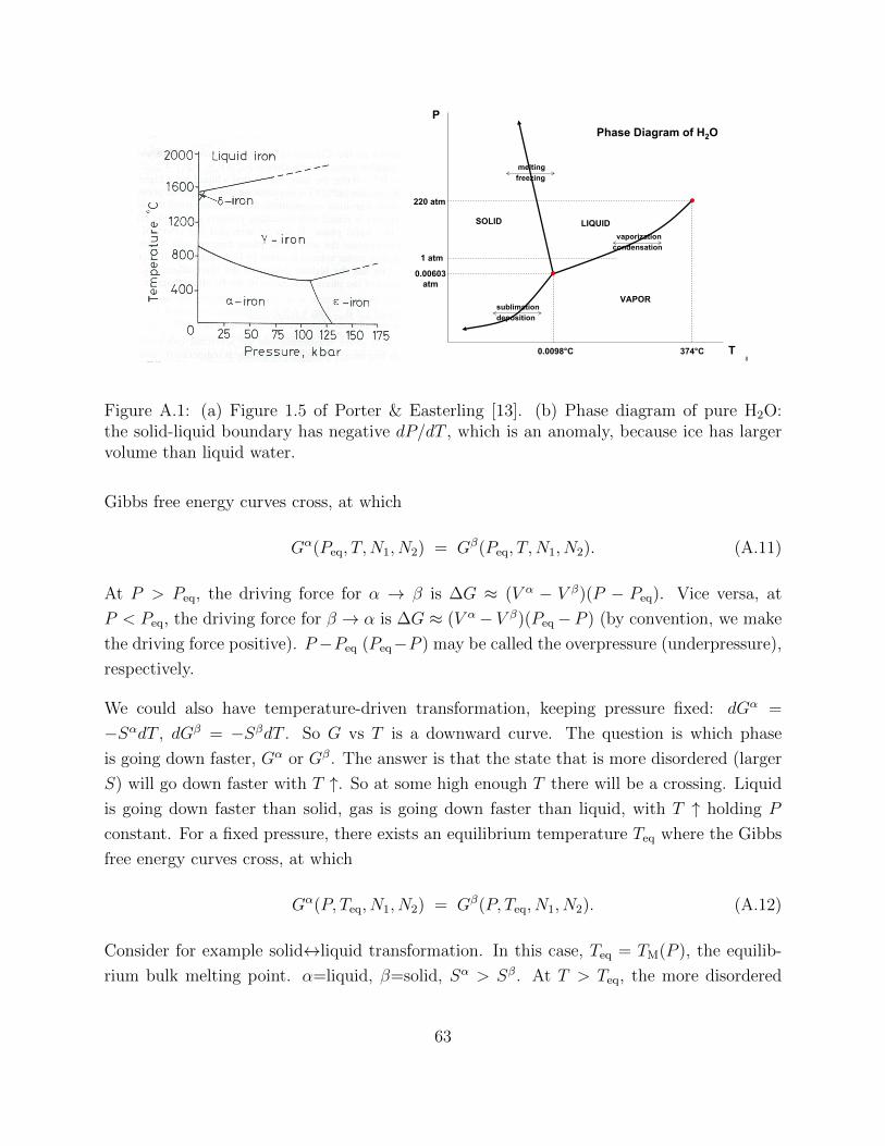
8
P
T0.0098°C
0.00603atm
SOLID
VAPOR
LIQUID
1 atm
220 atm
374°C
Phase Diagram of H2O
sublimationdeposition
vaporizationcondensation
meltingfreezing
Figure A.1: (a) Figure 1.5 of Porter & Easterling [13]. (b) Phase diagram of pure H2O:the solid-liquid boundary has negative dP/dT , which is an anomaly, because ice has largervolume than liquid water.
Gibbs free energy curves cross, at which
Gα(Peq, T,N1, N2) = Gβ(Peq, T,N1, N2). (A.11)
At P > Peq, the driving force for α → β is ∆G ≈ (V α − V β)(P − Peq). Vice versa, at
P < Peq, the driving force for β → α is ∆G ≈ (V α− V β)(Peq−P ) (by convention, we make
the driving force positive). P−Peq (Peq−P ) may be called the overpressure (underpressure),
respectively.
We could also have temperature-driven transformation, keeping pressure fixed: dGα =
−SαdT , dGβ = −SβdT . So G vs T is a downward curve. The question is which phase
is going down faster, Gα or Gβ. The answer is that the state that is more disordered (larger
S) will go down faster with T ↑. So at some high enough T there will be a crossing. Liquid
is going down faster than solid, gas is going down faster than liquid, with T ↑ holding P
constant. For a fixed pressure, there exists an equilibrium temperature Teq where the Gibbs
free energy curves cross, at which
Gα(P, Teq, N1, N2) = Gβ(P, Teq, N1, N2). (A.12)
Consider for example solid↔liquid transformation. In this case, Teq = TM(P ), the equilib-
rium bulk melting point. α=liquid, β=solid, Sα > Sβ. At T > Teq, the more disordered
63
phase is favored, and the driving force for β → α transformation, which is melting, is
∆G ≈ (Sα − Sβ)(T − TM). Vice versa at T < Teq, the more ordered phase is favored, which
is solidification, and the driving force for α → β is ∆G ≈ (Sα − Sβ)(TM − T ). Because we
are doing first-order expansion, it is OK to take Sα−Sβ to be the value at TM. However, at
TM we have Eα + PV α − TMSα = Hα − TMS
α = Hβ − TMSβ = Eβ + PV β − TMS
β, we have
Sα − Sβ = (Hα −Hβ)/TM. Hα −Hβ is in fact the heat released during phase change under
constant pressure, and is called the latent heat L. So we have
∆G ≈ L
TM
|TM − T |. (A.13)
|TM − T | is called undercooling / superheating for solidification / melting. We see that the
thermodynamic driving force for phase change is proportional to the amount of undercooling
/ superheating (in Kelvin), with proportionality factor LTM
= ∆S. Later we will see later
why a finite thermodynamic driving force is needed, in order to observe phase change within
a finite amount of time. (If you are extremely leisurely and have infinite amount of time,
you can observe phase change right at Teq).
solid/liquid: melting, freezing or solidification. liquid/vapor: vaporization, condensation.
solid/vapor: sublimation, deposition. At low enough pressure, the gas phase is going to
come down in free energy significantly, that the solid goes directly to gas, without going
through the liquid phase.
Thus, typically, high pressure / low temperature stabilizes solid phase, low pressure / high
temperature stabilizes gas phase. The tradeoff relation can be described by the Clausius-
Clapeyron relation for polymorphic phase transformation (single-component) in T − P
plane. The question we ask is that suppose you are already sitting on a particular (T, P )
point that reaches perfect equilibrium between α, β,
Gα(N1, N2, T, P ) = Gβ(N1, N2, T, P ) (A.14)
in which direction on the (T, P ) plane should one go, (T, P )→ (T+dT, P+dP ), to maintain
that equilibrium, i.e.:
Gα(N1, N2, T + dT, P + dP ) = Gβ(N1, N2, T + dT, P + dP ) (A.15)
Gα(N1, N2, T, P )− SαdT + V αdP = Gβ(N1, N2, T, P )− SβdT + V βdP. (A.16)
64
So:
−SαdT + V αdP = −SβdT + V βdP. (A.17)
and the direction is given by
dP
dT=
Sα − Sβ
V α − V β=
L
T (V α − V β). (A.18)
The above equation keeps one “on track” on the T − P phase diagram. It’s like in pitch
darkness, if you happen to stumble upon a rail, you can follow the rail to map out the whole
US railroad system. The Clausius-Clapeyron relation tells you how to follow that rail. L is
called “latent heat”. V α − V β is the volume of melting/vaporization/sublimation, you may
call it the “latent volume”.
In above we have only considered the scenario of so-called congruent transformation α↔ β,
where α and β are single phases with the same composition. We have not considered the
possibility of for example α ↔ β + γ, where γ has different composition or even structure
from β. To understand the driving force for such transformations which are indeed possible
in binary solutions, we need to further develop the language of chemical potential.
The total number of particles is N ≡ N1 + N2. Define mole fractions X1 ≡ N1/N , X2 ≡N2/N . Since there is always X1 + X2 = 1, we cannot regard X1 and X2 as independent
variables. Usually by convention one takes X2 to be the independent variable, so-called
composition. Composition is dimensionless, but it could be a multi-dimensional vector if
the number of species C > 2. For instance, in a ternary solution, C = 3, and composition
is a 2-dimensional vector X ≡ [X2, X3]. Composition can spatially vary in inhomogeneous
systems, for instance in an inhomogeneous binary solution, X2 = X2(x, t). In order for
α↔ β+γ to happen kinetically, for instance changing from X2(x) = 0.3 uniformly (initially
α phase) to some region with X2(x) = 0.5 (in β phase, “solute sink”) and some region with
X2(x) = 0.1 (in γ phase, ‘solute source”). This requires would require long-range diffusion
of type-2 solutes over distances on the order of the sizescale of the inhomogeneities, which
is called solute partitioning.
We can define the particle average Gibbs free energy to be g ≡ G/N = G(T, P,N1, N2)/(N1 +
N2). Like the chemical potentials, g will be minus a few eV in reference to isolated atoms
ensemble. It can be rigorously proven, but is indeed quite intuitively obvious, that g =
g(X2, T, P ), which is to say the particle average Gibbs free energy depends on chemistry
but not quantity (think of (N1, N2) ↔ (N,X2) as a variable transform that decomposes
65
dependent variables into quantity and chemistry). It is customary to plot g versus X2 at
constant T, P . It can be mathematically proven that µ1, µ2 are the tangent extrapolations
of g(X2) to X2 = 0 and X2 = 1, respectively. Algebraically this means
µ1(X2, T, P ) = g(X2, T, P ) +∂g
∂X2
∣∣∣∣∣T,P
(0−X2)
µ2(X2, T, P ) = g(X2, T, P ) +∂g
∂X2
∣∣∣∣∣T,P
(1−X2). (A.19)
It is also clear from the above that g(X2, T, P ) = X1µ1 +X2µ2, so
G(T, P,N1, N2) = N1µ1 +N1µ2 = N1∂G
∂N1
∣∣∣∣∣T,P,N2
+N2∂G
∂N2
∣∣∣∣∣T,P,N1
(A.20)
On first look, the above seems to imply that particle 1 and particle 2 do not interact. But
this is very far from true! In fact, µ1 = µ1(X2, T, P ), µ2 = µ2(X2, T, P ).
For pure systems: X2 = 0, g(X2 = 0, T, P ) = µ1(X2 = 0, T, P ) ≡ µ1(T, P ); or X2 = 1,
g(X2 = 1, T, P ) = µ2(X2 = 1, T, P ) ≡ µ2(T, P ). µ1(T, P ), µ2(T, P ) are called Raoultian
reference-state chemical potentials (they are not the isolated-atoms-in-vaccuum reference
states, but already as interacting-atoms). In this class we take the µ1, µ2 reference states to
the same structure as the solution, but in pure compositions (so-called Raoultian reference
states).
When plotted graphically, it is seen that g(X2) is typically convex up with µ1(X2, T, P ) <
µ1(T, P ) and µ2(X2, T, P ) < µ2(T, P ) (if not, what would happen?) This negative difference
is defined as the mixing chemical potential
µmixi ≡ µi(X2, T, P )− µi(T, P ), i = 1, 2 (A.21)
and mixing free energy
gmix ≡ X1µmix1 +X2µ
mix2 = g −X1µ1(T, P )−X2µ2(T, P ), Gmix = Ngmix (A.22)
respectively. Clearly, by definition, Gmix = 0 at pure competitions. gmix(X2, T, P ) can be
interpreted as the driving force to react pure 1 and pure 2 of the same structure as the
solution to obtain a solution of non-pure composition, per particle in the mixed solution.
∆G = −Ngmix(X2, T, P ) is in fact the chemical driving force to make a solution by mixing
66
pure constituents.
It turns out there exists “partial” version of the full differential (A.6):
dg(X2, T, P ) = vdP − sdT +∂g
∂X2
∣∣∣∣∣T,P
dX2 (A.23)
dµi(X2, T, P ) = vidP − sidT +∂µi∂X2
∣∣∣∣∣T,P
dX2 (A.24)
where
v1 ≡∂V
∂N1
∣∣∣∣∣T,P,N2
, v2 ≡∂V
∂N2
∣∣∣∣∣T,P,N1
, s1 ≡∂S
∂N1
∣∣∣∣∣T,P,N2
, s2 ≡∂S
∂N2
∣∣∣∣∣T,P,N1
,
e1 ≡∂E
∂N1
∣∣∣∣∣T,P,N2
, e2 ≡∂E
∂N2
∣∣∣∣∣T,P,N1
, h1 ≡∂H
∂N1
∣∣∣∣∣T,P,N2
, h2 ≡∂H
∂N2
∣∣∣∣∣T,P,N1
, ... (A.25)
Generally speaking, for arbitrary extensive quantity A (volume, energy, entropy, enthalpy,
Helmholtz free energy, Gibbs free energy), “particle partial A” is defined as:
ai ≡∂A
∂Ni
∣∣∣∣∣Nj 6=i,T,P
. (A.26)
The meaning of ai is the increase in energy, enthalpy, volume, entropy, etc. when an ad-
ditional type-i atom is added into the system, keeping the temperature and pressure fixed.
The particle-average a is simply
a ≡ A
N=
C∑i=1
Xiai. (A.27)
For instance, the particle average volume and particle average entropy
v ≡ V
N= X1v1 +X2v2, s ≡ S
N= X1s1 +X2s2, (A.28)
is simply the composition-weighted sum of particle partial volumes and partial entropies
of different-species atoms, respectively. While (A.27) relates all ai(X2, ..., XC , T, P )s to
a(X2, ..., XC , T, P ), it is also possible to obtain individual ai(X2, ..., XC , T, P ) from a(X2, ..., XC , T, P )
67
by the tangent extrapolation formula:
ai(X2, ..., XC , T, P ) = a(X2, ..., XC , T, P ) +C∑k=2
(δik −Xk)∂a(X2, ..., XC , T, P )
∂Xk
, (A.29)
where δik is the Kronecker delta: δik = 1 if i = k, and δik = 0 if i 6= k. Note in (A.29),
although the k-sum runs from 2 to C, i can take values 1 to C. (A.19) is a special case of
(A.29): for historical reason the particle partial Gibbs free energy is denoted by µi instead
of gi.
The so-called Gibbs-Duhem relation imposes constraint on the partial quantities when com-
position is varied while holding T, P fixed:
0 =C∑i=1
Xidai|T,P , (A.30)
For binary solution, this means
0 = X1dµ1|T,P +X2dµ2|T,P = X1dv1|T,P +X2dv2|T,P = X1ds1|T,P +X2ds2|T,P = ... (A.31)
The above can be proven, but we will not do it here.
The above is the general solution thermodynamics framework. To proceed further, we need
some detailed models of how g depends on X2. In so-called ideal solution:
µideal−mix1 (X2, T, P ) = kBT lnX1, µideal−mix
2 (X2, T, P ) = kBT lnX2. (A.32)
And so
gideal−mix(X2, T, P ) ≡ kBT (X1 lnX1 +X2 lnX2), (A.33)
which is a symmetric function that is always negative (that is to say it always prefer mixing),
with −∞ slope on both sides. Ideal solution is realized nearly exactly in isotopic solutions
such as 235U - 238U. In such case, there is no chemical difference between the two species
(εAA = εBB = εAB), so the enthalpy of mixing is zero. The driving force for mixing is
entirely entropic in origin, because there would be many ways to arrange 235U and 238U
atoms on a lattice, whereas there is just one in pure 235U or pure 238U crystal (235U atoms
are indistinguishable among themselves, and so are 238U atoms). This can be verified from
the formula smix = −∂gmix/∂T , hmix = ∂(gmix/T )/∂(1/T ).
68
We define excess as difference between the actual mix and the ideal-mix functions:
gexcess ≡ gmix(X2, T, P )− gideal−mix(X2, T, P ), µexcessi ≡ µmix
i − kBT lnXi. (A.34)
Clearly, excess quantities for ideal solution is zero.
In so-called regular solution model,
gexcess(X2, T, P ) = ωX1X2, (A.35)
where ω is X2,T ,P independent constant. Using (A.19), we get
µexcess1 = ωX2
2 , µexcess2 = ωX2
1 . (A.36)
And so
µ1(X2) = µ1 + kBT lnX1 + ωX22 , µ2(X2) = µ2 + kBT lnX2 + ωX2
1 . (A.37)
It is also customary to define activity coefficient γi, so that
µi(X2, T ) ≡ µi(T ) + kBT ln γiXi. (A.38)
Contrasting with (A.37), we see that in the regular solution model, the activity coefficients
are γ2(X2, T ) = eωX21/kBT , γ1(X2, T ) = eωX
22/kBT .
When ω < 0, the driving force for mixing is greater than in ideal solution. When one uses
the formula s = −∂g/∂T , h = ∂(g/T )/∂(1/T ), we can see that the ideal-mixing contribution
is entirely entropic, whereas the excess contribution is entirely enthalpic if ω is independent
of temperature. In fact, it can be shown from statistical mechanics that
ω = Z ((εAA + εBB)/2− εAB) , (A.39)
where εAB is the Kossel spring binding energy between A-B (“heteropolar bond”), and εAA
and εBB are the Kossel spring binding energy between A-A and B-B (homopolar bonds).
Derivation of the regular solution model (this has been shown in MSE530 Thermody-
namics of Materials): arrange XAN A atoms and XBN B atoms on a lattice. The number
69
of choices:
Ω =N !
(XAN)!(XBN !)(A.40)
Assume all these choices (microstates) have the same enthalpy:
H = −Z(XAN(XBεAB +XAεAA) +XBN(XBεBB +XAεAB))/2
= −NZ(2XAXBεAB +X2AεAA +X2
BεBB)/2 (A.41)
in contrast to reference state of pure A and pure B
Href = −NZ(XAεAA +XBεBB)/2 (A.42)
so the excess is:
Hexcess = −NZ(2XAXBεAB +X2AεAA −XAεAA +X2
BεBB −XBεBB)/2
= −NZ(2XAXBεAB −XAXBεAA −XBXAεBB)/2
= NZXAXB ((εAA + εBB)/2− εAB) = NωXAXB. (A.43)
According to the Boltzmann formula S = kB ln Ω, the entropy is
S = kB lnN !
(XAN)!(XBN !)≈ kB(N lnN −XAN lnXAN −XBN lnXBN)
= −NkB(XA lnXA +XB lnXB), (A.44)
using the Stirling formula: lnN ! ≈ N lnN − N for large N . S is the same as that in ideal
solution, because the regular solution model takes the “mean-field” view that all possible
configurations are iso-energetic. The regular solution model in the form of (A.35) is a well-
posed model with algebraic simplicity, but it may not reflect reality very well.
For positive ω, spinodal decomposition will happen below a critical temperature TC: a
random 50%-50% A-B solution α would separate into A-rich solution α1 and B-rich solution
α2 - see plots of g(X2, T ) at different T . We have studied this model in detail in MSE530.
For negative ω, although nothing will happen as seen from the regular solution model, in
reality order-disorder transition will happen below a critical temperature TC, where the
A-B solution starts to posses chemical long-range order (CLRO). A good example is β-
brass, a Cu-Zn alloy in BCC structure (Z = 8). See Chap. 17 of [14]. Cu and Zn atoms like
each other energetically, more than Cu-Cu, and Zn-Zn. Suppose XZn = 0.5, at T = 0, what
70
would be the optimal microscopic configuration? Since F = E−TS, at T = 0 minimization
of F is the same as minimization of E = U , the system will try to maximize the number of Cu-
Zn bonds. Indeed, so-called long-range chemical order, that is, Cu occupying one sub-lattice
(’) and Zn occupying another sub-lattice (”), or Cu occupying sub-lattice ” and Zn occupying
sub-lattice ’ would give the maximum number of Cu-Zn bonds. The regular solution model
did not distinguish between the two sub-lattices, statistically speaking. In order to be able
to distinguish, let us define sub-lattice compositions X ′A + X ′B = 1, X ′′A + X ′′B = 1. Clearly
the overall composition
XA =1
2(X ′A +X ′′A), XB =
1
2(X ′B +X ′′B). (A.45)
By defining sub-lattice compositions, we have effectively added one more “coarse” degree of
freedom to describe our alloy, the so-called η order parameter:
η ≡ 1
2(X ′′B −X ′B). (A.46)
Cu50Zn50 taking the CsCl structure at T = 0 would have η = 0.5 or η = −0.5. Previously, the
regular solution model constrains η = 0 (because it does not entertain an η order parameter).
Now, with η, we would have
X ′′B = XB + η, X ′B = XB − η, X ′′A = 1−XB − η, X ′A = 1−XB + η. (A.47)
Still under the mean-field approximation (so called Bragg-Williams approach [15, 16] in
alloy thermochemistry), as the regular solution model, we can estimate the proportion of
A(’)-A(”) bonds:
pAA = X ′′AX′A = (1−XB − η)(1−XB + η), (A.48)
the proportion of B(’)-B(”) bonds:
pBB = X ′′BX′B = (XB + η)(XB − η), (A.49)
the proportion of A(’)-B(”) bonds:
pAB = X ′AX′′B = (1−XB + η)(XB + η), (A.50)
71
the proportion of A(”)-B(’) bonds:
pBA = X ′BX′′A = (XB − η)(1−XB − η) (A.51)
among all the nearest-neighbor bonds in the alloy. Clearly, the above Bragg-Williams esti-
mation satisfies the sum rule constraint:
pAA + pBB + pAB + pBA = 1. (A.52)
The particle-average energy is thus just
h = −Z2
(pAAεAA + pBBεBB + (pAB + pBA)εAB) (A.53)
From derivations of the regular solution model and discussions in the last semester, we
see that if we chose our reference state appropriately, then we can say εAA = 0, εBB = 0,
εAB = −ω/Z, to simplify the algebra:
h(XB, η) = ω(XAXB + η2). (A.54)
which we see is the same as the regular solution model if η = 0. The physics of the above
expression is that, if with CLRO and solute partitioning onto the two sub-lattices, one can
increase the number of A-B bonds from XAXB to XAXB + η2.
The entropy is just the sum of the entropies of the two sub-lattices (in other words, the total
number of possible microstates is the product of the numbers of microstates on ’ sublattice
and that on ” sublattice). Therefore:
s(XB, η) = −kB
2(X ′A lnX ′A +X ′B lnX ′B +X ′′A lnX ′′A +X ′′B lnX ′′B). (A.55)
The free energy (of mixing) per particle is thus
g(XB, η) = ω(XAXB + η2) +kBT
2(X ′A lnX ′A +X ′B lnX ′B +X ′′A lnX ′′A +X ′′B lnX ′′B) (A.56)
with∂g
∂η= 2ωη +
kBT
2
(− ln
X ′BX ′A
+ lnX ′′BX ′′A
), (A.57)
72
∂2g
∂η2= 2ω +
kBT
2
(1
X ′BX′A
+1
X ′′BX′′A
). (A.58)
In a real material, both XB and η are fields: g(XB(x, t), η(x, t)). However, we note there is
a fundamental difference between XB and η. XB(x, t) is conserved:∫dxXB(x, t) = const (A.59)
if integration is carried out in the entire space. Thus, when optimizing
G =1
Ω
∫dxg(XB(x), η(x)) (A.60)
we can not do an unconstrained optimization on g(XB): there has to be a Lagrange mul-
tiplier (the chemical potential) on the total free energy minimization. On the other hand,
there is no such constraint on η: we can do an unconstrained optimization with respect to η
(and indeed that is what Nature does). More involved discussions [14] show that XB is so-
called conserved order parameter, and evolve according to the so-called Cahn-Hilliard
evolution equation [17] (basically diffusion equation), whereas non-conserved order pa-
rameter like the CLRO evolve according to the so-called Allen-Cahn equation [18], in the
linear response regime.
For a given T,XB, we thus have
g(XB) = minηg(XB, η) (A.61)
at thermodynamic equilibrium. So:
ln(XB − η)(1−XB − η)
(XB + η)(1−XB + η)=
4ωη
kBT(A.62)
We note that η = 0 is always a solution to above, i.e. it is always a stationary point in the
variational problem. But is η = 0 a minimum or a maximum? From (A.58) we note that at
high enough T , η = 0 would always be a free energy minimum. But as T cools down, at
TC(XB) =−2ωXB(1−XB)
kB
(A.63)
g(XB, η) would lose stability with respect to η at η = 0, in a manner of 2nd order phase trans-
formation (for example, magnetization at Curie temperature). This is called order-disorder
73
transformation, where chemical long-range order emerges at a low enough temperature. In
particular, the highest temperature where chemical order may emerge is at XB = 0.5, where
the enthalpic driving force for two sub-lattice partition is especially strong:
T ∗C = − ω
2kB
. (A.64)
We also note that T ∗C exists only for ω < 0. If ω > 0, ∂2g∂η2
> 0 always and η = 0 stays stable
global minimum. Thus the Bragg-Williams model is the same as the regular solution model
for ω > 0. The Bragg-Williams model gives only different results from the regular solution
model for ω < 0, and in that case for
T < TC(XB) = 4T ∗CXB(1−XB) (A.65)
only. At T < TC(XB), we have the CLRO at equilibrium:
ln(XB + η)(1−XB + η)
(XB − η)(1−XB − η)=
8ηT ∗CT
, (A.66)
from which we can solve for η.
The above is called the Bragg-Williams approach, which is at the same level of theory (mean-
field approximation) as the regular solution model, and only gives different results (η 6= 0)
if ω < 0 and T < TC. There are certain solid-state chemistries where ω is very negative,
in which case CLRO is close to the maximum possible value for a large temperature range.
These are so-called line compounds (because off-stoichiometry solubility range is so low,
these phases appear as lines in T − X2 phase diagrams) or ordered phases, with formulas
like AmBn where m and n are integers. Many crystalline ceramics (oxides, nitrides, carbides
etc.) are line compounds, as the solubility range is typically very narrow besides the ideal
stoichiometry. In metallic alloys, these would be called intermetallics compound phases.
These phases are typically very strong mechanically (stability due to very negative ω), and
are used as strengthening phases (precipitates) to impede dislocation motion. There are
special symbols to denote these phases with long-range chemical order, such as L20 (bcc
based), L12 (fcc based), L10 (fcc based), D03, D019, Laves phases, etc.
There is still a higher-level of theory called the quasi-chemical approximation [5, 19],
originating from a series of approximations by Edward A. Guggenheim [10]. It proposes the
concept of chemical short-range order (CSRO): even in so-called random solid solution
(ω > 0, or ω < 0 but T > TC) which has no long-range chemical order, η = 0, the atomic
74
arrangements may not be random as in the mean-field sense, and manifest “correlations”. For
example, a pair “correlation” means the probability of finding a particular kind of A-B bond
is larger than the product of average probabilities of finding A in a particular sublattice and
B in another sublattice. Beyond pair correlations, there are also triplet correlations, quartet
correlations, ..., in a so-called cluster expansion approach [12], each addressing an excess
probability beyond the last level of theory. Specifically, in the quasi-chemical approximation
one uses the pair probabilities pAA, pBB, pAB, pBA as coarse degrees of freedom. These are
valid order parameters, because at least in principle one could count the fraction of A(’)-
A(”), B(’)-B(”), A(’)-B(”), A(”)-B(’) bonds in a given RVE. These coarse-grained statistical
descriptors will take certain values, and one can formulate a variational problem based on
them.
pAA, pBB, pAB, pBA must satisfy sum rule (A.52). Therefore, in addition to XB, η, the
quasi-chemical approximation introduces three more degrees of freedom. In systems where
CLRO vanish, there is no statistical distinction between the two sub-lattices, so pAB = pBA,
in which case only two additional degrees of freedom from the quasi-chemical approach. The
quasi-chemical free energy reads:
g(XB, η, pAB, pBA, pBB) =ω(pAB + pBA)
2+
kBT
2(X ′A lnX ′A +X ′B lnX ′B +X ′′A lnX ′′A +X ′′B lnX ′′B) +
ZkBT
2(pBB ln
pBB
X ′BX′′B
+ pAB lnpAB
X ′AX′′B
+ pBA lnpBA
X ′BX′′A
+
(1− pBB − pAB − pBA) ln1− pBB − pAB − pBA
X ′AX′′A
) (A.67)
with sub-lattice compositions X ′A, X ′′A, X ′B, X ′′B taken from (A.47) The actual chemical free
energy at local equilibrium is
g(XB) = minη,pAB,pBA,pBB
g(XB, η, pAB, pBA, pBB) (A.68)
As a general remark, a compound phase would tend to manifest as sharp “needle” in g(XB),
which means small deviation from the ideal stoichiometry AmBn would cause large “pain”
or increase in g(XB), since A-A and B-B bonds must be formed (due to the host lattice
structure) which are much more energetically costly than A-B bonds.
Both spinodal decomposition and order-disorder transformation are 2nd-order phase trans-
75
formations, defined by a vanishingly small jump in the order parameter, as one crosses the
transition temperature TC. In contrast, 1st-order phase transition are characterized by a
finite jump in order parameter. For instance, in melting, we can use the local density as
order parameter to distinguish between liquid and solid, or some feature of the selected area
electron diffraction (SAED) pattern. In either case, before and after melting, there is a finite
jump in this order parameter field (ρ(x, T−melt) = ρs but ρ(x, T+melt) = ρl for some x). Thus,
melting is a 1st-order phase transitions. Also, consider an eutectic decomposition reaction:
l→ α+β, defined by (TE, X lE2 , X
αE2 , XβE
2 ). If one uses the local composition as the order pa-
rameter: then there is also a finite change (X2(x, TE+) = X lE2 but X2(x, TE−) = XαE
2 or XβE2 ,
for some x). In contrast, in the case of ω > 0 and spinodal decomposition α→ α1 +α2 which
is 2nd-order phase transformations, Xα22 −Xα1
2 ∝√TC − T . Whereas X2(x, T−C ) = Xα
2 uni-
formly T+C , one sees only infinitesimal compositional modulations at T−C : X2(x, T−C ) = Xα1
2
or Xα22 . The amplitude of the concentration wave (concentration is our order parameter
here) is infinitesimal.
Common tangent construction: µα2 (Xα2 , T ) = µβ2 (Xβ
2 , T ), µα1 (Xα2 , T ) = µβ1 (Xβ
2 , T ) manifest
as common tangent between gα(X2) and gβ(X2) curves. This equation has two unknowns,
Xα2 and Xβ
2 , and we need to solve two joint equations which are generally nonlinear (thus nu-
merical solution by computer may be needed). Show graphically how this may be established
for two phases α, β, rich in A and B, respectively, by diffusion. Since
dG = V dP − SdT +C∑i=1
µidNi, (A.69)
atoms/molecules will always migrate from high chemical potential phase/condition to low
chemical potential phase/condition.
Let us now investigate situations where a large-solubility phase (α) is in contact with a
line compound phase (β). The common tangent construction can be simplified in these
situations. Let us consider two limiting cases (a) and (b), where the gβ(X2, T ) needle is
“around” (a) X2 ≈ 0 and (b) X2 ≈ 1, respectively. (a) corresponds to an example of adding
antifreeze to water, where the liquid solution delays freezing due to addition of solutes. (b)
corresponds to an unknown solubility problem, which is to say how much can be dissolved
in α for a given temperature when it is interfaced with a precipitate β phase that is nearly
pure 2.
(a): people add antifreeze to say liquid water, to suppress the freezing temperature. How
76
does that work?
In this case, gβ(X2, T ) is a needle “around” X2 ≈ 0 (the ice phase), whereas α is the liquid
phase. The first thing to realize is the solubility of B is typically lower in solids than in
liquids. Energetic interaction between atoms is more important in solids than liquids, since
atoms in solids are bit closer in distance, and also put a premium on periodic packing.
“Misfit” molecules B would feel much more comfortable living in a chaotic environment
like liquid, than in a crystal (think about societal analogies). To first approximation, we
can assume the ice crystals that first precipitates out as temperature is cooled is pure ice:
µiceH2O(X ice
B , T, P ) ≈ µiceH2O(T, P ).
The second thing to realize is that
µliquidH2O ≈ µliquid
H2O (T, P ) + kBT lnX liquidH2O (A.70)
If the ≈ in above is =, then it is an ideal solution. Raoult’s law says that no matter what
kind of solution (solid,liquid,gas), as long as the solutes become dilute enough, the solvent
molecule’s chemical potential approaches that in an ideal solution. This is in fact also true
for the ice crystals, but X iceB is so small that it’s not going to have any effect on H2O in ice.
For the liquid, we have
lnX liquidH2O = ln(1−X liquid
B ) ≈ −X liquidB . (A.71)
So the chemical potential of water in liquid solution is lowered by X liquidB kBT due to the
presence of B in liquid. How much does that lower the melting point? (compared to what?)
µliquidH2O (T, P )− kBTX
liquidB = µice
H2O(T, P ) (A.72)
Remember that T puremelt is defined by
µliquidH2O (T pure
melt , P ) = µiceH2O(T pure
melt , P ). (A.73)
Perform Taylor expansion with respect to T :
−∆spuremelt(T − T
puremelt ) = kBTX
liquidB , (A.74)
we get
T puremelt − T ≈
kBTpuremelt
∆spuremelt
X liquidB . (A.75)
77
The pure liquid with larger entropy of melting will have less relative melting point suppression
(essentially steeper µi(T ) will be less sensitive). What is interesting about (A.75) is that the
potency of an antifreeze is independent of the chemical type of the antifreeze, at least when
only a tiny amount of antifreeze is added. When the solution is very dilute, the stabilization
of the solvent is entirely entropic.
Richard’s rule: simple metals have ∆spuremelt ≈ 1− 2kB. Water has ∆spure
melt ≈ 2.65kB.
Trouton’s rule: ∆spureevap ≈ 10.5kB, for various kinds of liquids. Water has ∆spure
evap ≈ 13.1kB.
Now consider the opposite limit (b): in this case, gβ(X2, T ) is a needle around X2 ≈ 1. Then
for a given T , gβ(Xβ2 , T ) ≈ µβ2 (Xβ
2 , T ) ≈ µβ2 (T ), and we just need to solve
µα2 (Xα2 , T ) = µβ2 (T ) (A.76)
It can be shown mathematically, but is quite obvious visually, that the second equation
µα1 (Xα2 , T ) = µβ1 (Xβ
2 , T ) for the solvent atoms becomes “unimportant” (still rigorously true,
just that whether we solve it or not has little bearing on what we care about - one can draw
a bunch of tangent extrapolations on gβ(Xβ2 ) with slight differences in Xβ
2 , we can see huge
changes in µβ1 but little changes in µβ2 , due to the vast difference in extrapolation distances -
such equations are called “stiff” - stiff equations can make analytical approaches easier, but
general numerical approaches more difficult). So we have effectively reduced to 1 unknown
and 1 equation (or rather, we have decoupled a previously 2-unknowns-and-2-equations into
two nearly indepedent 1-unknown-and-1-equations).
Suppose α=simple cubic, β=BCC. Suppose α phase can be described by regular solution
with ω > 0 (see Fig. 1.36 of [13], there is an eutectic phase diagram and gα(Xβ2 ) bulges out
in the middle):
µα2 (T ) + kBT lnXα2 + ω(1−Xα
2 )2 = µβ2 (T ) (A.77)
Rearranging the terms we get
Xα2 = exp
(− µ
α2 (T )− µβ2 (T ) + ω(1−Xα
2 )2
kBT
)(A.78)
The above can be solved iteratively. We first plug in Xα2 = 0 on RHS, get a finite Xα
2 on the
LHS, then plug this new Xα2 to RHS and iterate. From the very first iteration, however, we
78
get
Xα2 = exp
(− µ
α2 (T )− µβ2 (T ) + ω
kBT
)(A.79)
and if Q(T ) ≡ µα2 (T ) − µβ2 (T ) + ω kBT , Xα2 would be small and then the first iteration
would be close enough to convergence. µα2 (T )− µβ2 (T ) is how much more uncomfortable it is
for a type-2 atom to be living in pure-2 α structure compared to pure-2 β structure. ω is still
how much more uncomfortable it is for type-2 atom to be living among a vast sea of type-1
atoms rather than among its own kind (at 0K, µα2 = −Zαε22/2, ω = Zα(−ε12 +(ε11 + ε22)/2),
so µα2 + ω = Zα(−ε12) − (−Zαε11/2), which corresponds to the process of squeezing out
a type-1 atom and placing it on a ridge, then inserting a type-2 atom into this sea of 1).
Thus Q(T ) is an energy that can be interpreted as how much more uncomfortable it is to
transfer a B atom from pure β phase to dilute α phase, excluding the configurational entropy
of B in α phase. Exponential forms of the kind e−Q/kBT are called Boltzmann distribution
in thermodynamics, and Arrhenius expression when one talks about rates in kinetics. It
says that even though some places are (very) uncomfortable to be at or somethings are
(very) difficult to do, there will always be some fraction of the population who will do those,
because thermal fluctuations reward disorder and risk-taking. A prominent feature of these
Boltzmann/Arrhenius forms, especially at low temperatures, is that kBT in the denominator
is a very violent term. A change in T by 100C can conceivably cause many orders of
magnitude change in the solubility.
The above train of thought can be extended to vacancies. A monatomic crystal made of
type-A atoms, but with the possibility of “porosity” inside (non-occupancy of lattice sites),
can be regarded as a fully dense A-B crystal with B identified as “Vacadium”. In this case,
εBB = εAB = 0, so ω = ZεAA/2, i.e. it is enthalpically costly to mix Vacadium with A, and
they would prefer to segregate if based entirely from enthalpy standpoint or at T = 0 K.
However, entropically A and Vacadium would prefer to mix. When you mix a block of pure
Vacadium (in β phase) with pure A in α (fully dense), the solubility of Vacadium in α would
be XV = e−Q/kBT . Also, when you are 100% Vacadium it does not matter what structure the
Vacadium atoms are arranged, so µα2 (T )− µβ2 (T ) = 0 thus Q = ω = ZεAA/2. Q is called the
vacancy formation energy in this context. Physically, Q is identified as the energy cost to
extract an atom from lattice (break Z bonds) and attach it to an ledge on surface (form Z/2
bonds), in a Kossel crystal. In this class the above process is called the canonical vacancy
creation process. The canonical vacancy creation process creates porosity inside the solid,
making the solid appear larger than the fully dense state (social analogy would be “hype”).
Note that the canonical vacancy creation process is not an atomization process, where one
79
extracts an atom and put it away to infinity.
An abstract view of phase transformation. Define order parameter η, which could be density,
structure factor, magnetic moment, electric polarization, etc. η is a scalar of your choice
that best reflects the nature of the problem (phase transition). The Gibbs free energy is
defined as G(N1, N2, ..., NC , T, P ; η). There are global minimum, metastable minima, and
saddle point. For example, at low temperature, for pure iron, both G(ηFCC) and G(ηBCC) are
local minima of G(η), but G(ηFCC) > G(ηBCC). To go from η1 = ηFCC to η2 = ηBCC, G(η)
must first go even higher than G(η1). This energy penalty is called the activation energy,
and η ∈ (η1, η2) is called the reaction coordinate. Define η∗ to be the position of saddle
point, we have
Q1→2 = G(η∗)−G(η1), Q2→1 = G(η∗)−G(η2). (A.80)
According to statistical mechanics, all possible states of η can exist, just with different
probability. The rate of transition, if one is at η1, to η2, is given by:
R1→2 = ν0 exp(−Q1→2
kBT), (A.81)
where ν0 is some attempt frequency (unit 1/s), corresponding to the oscillation frequency
around η1 (imagine a harmonic oscillator coupled to heat bath). The rate of transition, if
one is already at η2, to η1, is given by:
R2→1 = ν0 exp(−Q2→1
kBT
). (A.82)
If G(η1) > G(η2), then Q1→2 < Q2→1, and R1→2 R2→1 since Q’s are in the exponential,
and Q2→1 −Q1→2 = G(η1)−G(η2) is proportional to the sample size.
One can also express η as function of position, η(x), to represent an interface. Consider
the condition when FCC is in equilibrium with BCC: G(ηFCC) = G(ηBCC), and there is an
interface that separates them. η(x) is then a sigmoid-like curve, with characteristic width
defined as interfacial width. The interfacial energy arises because atoms in the interface are
neither FCC or BCC, and have energy density higher than either of them. This would lead
to a positive interfacial energy (Chap. 3)
The common tangent construction gives unique solution in composition when T, P is fixed.
If T, P come into play, however, then the game is richer. The single-component Clausius-
Clapeyron relation (A.18) can be generalized to C-component solutions. If we consider i in
80
α of composition Xα ≡ [Xα2 , ..., X
αC ], or in β of composition Xβ ≡ [Xβ
2 , ..., XβC ], there needs
to be
µαi (Xα, T, P ) = µβi (Xβ, T, P ) (A.83)
to maintain mass action equilibrium (chemical equilibrium), to make sure atom i is “equally
happy” in α as in β. Let us investigate what dP/dT needs to be in order to maintain that
way, if Xα and Xβ are fixed (for instance two “compound” phases, or one compound phase
in contact with a large constant-composition reservoir): because we have
dµαi = vαi dP − sαi dT, dµβi = vβi dP − sβi dT. (A.84)
To maintain (A.83), we need
dP
dT=
sαi − sβi
vαi − vβi
=hαi − h
βi
T (vαi − vβi ), (A.85)
the latter equality is because if α, β are already at chemical equilibrium for i at a certain
(T, P ), there is:
µαi = hαi − Tsαi = µβi = hβi − Tsβi . (A.86)
Consider for example, the equilibria between pure liquid water (β) and air (α): air is a
solution. Then one has:dP
dT≈ hαi − h
βi
T (vαi )(A.87)
since vαi is larger than vβi by a factor of 103. For the air solution N = (N1, N2, N3, ...Nc), we
have
V ≈ NkBT
P→ vi ≡
∂V
∂Ni
∣∣∣∣∣Nj 6=i,T,P
=kBT
P. (A.88)
ThusdP
dT≈ hαi − h
βi
T (kBT/P ),
d lnP
d(1/T 2)≈ −∆hi
kB
. (A.89)
So:
lnP eq
P eqref
≈ ∆hikB
(1
Tref
− 1
T
), (A.90)
when temperature is raised, the equilibrium vapor pressure goes up.
Notice that the gas phase always beats all condensed phases at low enough (but still positive)
pressure. One can thus draw a lnP -T diagram, and down under it is always the gas phase.
81
This is because chemical potential in the gas phase goes as
µgasi (Xgas, T, P ) ≈ kBT lnXiP + µgas
i (T, 1atm), (A.91)
which goes to −∞ as P → 0, whereas chemical potentials in condensed phases are bounded.
(The physical reason for going to −∞ as P → 0 is that the entropy of gas blows up as
kB ln v). Thus, all condensed phases (liquid,solid) become metastable at low enough pressure
(see water phase diagram, Fig. A.1 (b)). Another way of saying it is that there always exists
an equilibrium vapor pressure for any temperature and composition, which may be small but
always positive, below which components in the liquid or solid solution would rather prefer
to come out into the gas phase (volatility).
However, they are two manners by which vapor can come out. When you heat up a pot
of water, at say 80C, you can already feel vapor coming out if you stand over the pot,
and maybe see some steam, but it’s very peaceful evaporation process. However, when the
temperature reaches 100C, there is a very sharp transition. Suddenly there is a lot of
commotion, and there is boiling. What defines the boiling transition?
The commotion is caused by the presence of gas bubbles, not present before T reaches Tboil.
The boiling transition is defined by P eq = 1 atm, the atmospheric pressure. Before T < Tboil,
there may be P eq > P ambientH2O , so the water molecules would like to come out. But they can
only come out from the gas-liquid interface, not inside the liquid, so the evaporation action is
limited only to the water molecules in the narrow interfacial region < 1nm. This is because
any pure H2O gas bubbles formed inside would be crushed by the hydrostatic pressure AND
surface tension. But when P eq > 1 atm, pure H2O gas bubbles can now nucleate inside the
liquid. These bubbles nucleate, grow, and eventually rise up and break. At T > Tboil the
whole body of liquid can join the action of phase transformation, not just the lucky few near
the gas-liquid interface. Thermodynamically, there is nothing very special about the boiling
transition, but if you look at the rate of water vapor coming out, there is a drastic upturn at
T = Tboil. So the boiling transition is a transition in kinetics. The availability of nucleation
sites is important for such kinetic transitions. In the case of boiling, the nucleation sites
are likely to be the container wall (watch a bottle of coke). Without the heterogeneous
nucleation sites, it is possible to significantly superheat the liquid past its boiling point,
without seeing the bubbles.
One can have superheating/supercooling because of the barriers to transformation. The
82
amount of thermodynamic driving force in a temperature-driven phase transformation is:
∆G ≡ µαi − µβi ≡ ∆µi ≈ ∆seq
i ∆T =∆heq
i
T eq∆T (A.92)
if the reaction coordinate is identified as mass transfer from one phase to another (η1 state:
Nαi + 1 in α, Nβ
i in β; η2 state: Nαi in α, Nβ
i + 1 in β). To drive kinetics at a finite speed,
the driving force (thermodynamic potential loss or dissipation) must be finite.
83
Appendix B
Interfaces
Interfaces such as grain boundaries, phase boundaries (free surface is the phase boundary
between condensed and vapor phase), stacking faults, domain walls are locations where 3D
order parameter field (phase field) sustains a finite jump. They are extended defects like
the dislocations, and therefore do not have an equilibrium distribution. In other words,
they must be produced as a cause of dissipative processes (mechanical work done, radiation,
thermal quench) that gives rise to emergent behavior.
B.1 Interfacial Segregation
Gibbs developed the theory of chemical potential for homogeneous 3D phases in 1870s at
Yale, but he also thought about the problem of interfaces very carefully. At his time there
was no instrument that could directly visualize the atoms in the interface. But by the power
of imagination Gibbs developed the concept of interfacial excesses and Gibbs Adsorption
Equation.
Gibbs developed the theory for interface between α, β phases under the following assump-
tions: (a) spatial inhomogeneity only exists near the physical interface region, which is very
thin; away from the interfaces, both phases are homogeneous with particle concentrations
cα and cβ, respectively. (b) both α and β are fluid phases that can only sustain hydrostatic
pressures. Away from the physical interface region, the hydrostatic pressures are Pα and
P β, respectively.
84
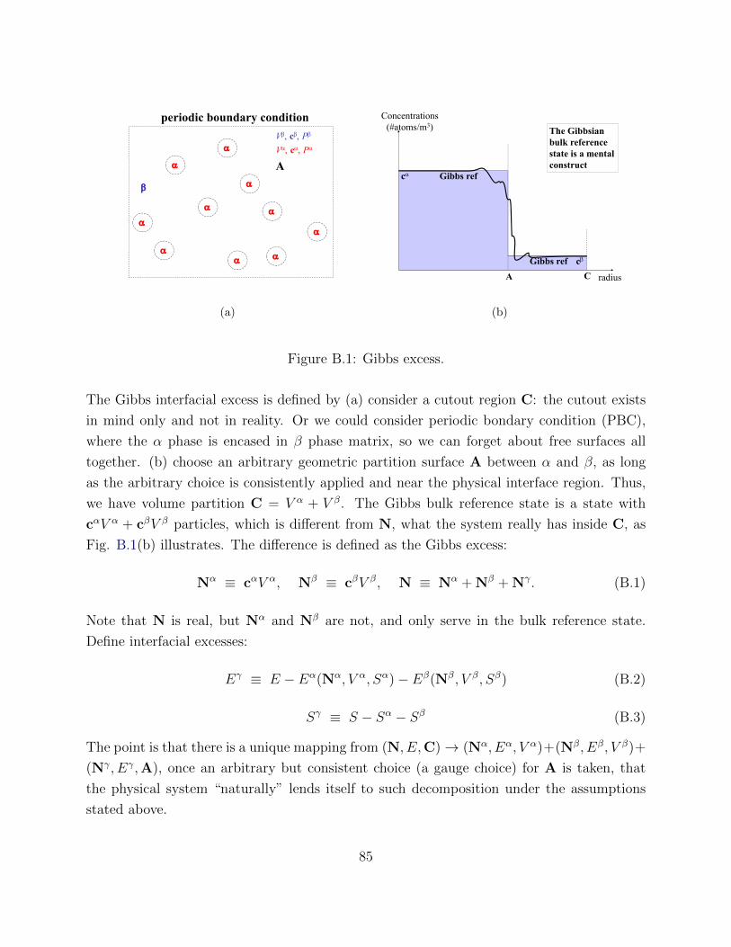
periodic boundary condition
VcPVcP
A
(a)
radius
Concentrations(#atoms/m3)
A
c
c
Gibbs ref
Gibbs refC
The Gibbsianbulk reference state is a mental construct
(b)
Figure B.1: Gibbs excess.
The Gibbs interfacial excess is defined by (a) consider a cutout region C: the cutout exists
in mind only and not in reality. Or we could consider periodic bondary condition (PBC),
where the α phase is encased in β phase matrix, so we can forget about free surfaces all
together. (b) choose an arbitrary geometric partition surface A between α and β, as long
as the arbitrary choice is consistently applied and near the physical interface region. Thus,
we have volume partition C = V α + V β. The Gibbs bulk reference state is a state with
cαV α + cβV β particles, which is different from N, what the system really has inside C, as
Fig. B.1(b) illustrates. The difference is defined as the Gibbs excess:
Nα ≡ cαV α, Nβ ≡ cβV β, N ≡ Nα + Nβ + Nγ. (B.1)
Note that N is real, but Nα and Nβ are not, and only serve in the bulk reference state.
Define interfacial excesses:
Eγ ≡ E − Eα(Nα, V α, Sα)− Eβ(Nβ, V β, Sβ) (B.2)
Sγ ≡ S − Sα − Sβ (B.3)
The point is that there is a unique mapping from (N, E,C)→ (Nα, Eα, V α)+(Nβ, Eβ, V β)+
(Nγ, Eγ,A), once an arbitrary but consistent choice (a gauge choice) for A is taken, that
the physical system “naturally” lends itself to such decomposition under the assumptions
stated above.
85
For the physical system, when C and A is fixed,
dE = TdS +∑i
µidNi, (B.4)
for the injection of heat and particles into C. Let them equilibrate inside C, and remeasure
(Sα,Nα), (Sβ,Nβ), and recalculate the tracking reference quantities:
dEα = TdSα +∑i
µidNαi , dEβ = TdSβ +
∑i
µidNβi (B.5)
recognizing the intensive quantities T and µi are the same everywhere in the physical system,
and that the reference system and the physical system agree in these intensive quantities.
So we have:
dEγ = TdSγ +∑i
µidNγi . (B.6)
In essence, the perspective is to map the physical system, which has small but finite interfacial
thickness, to a fictitious system of three phases α, β, γ, where γ has zero volume but finite
particle number and energy as well as entropy.
The γ phase does have finite area A, which can vary as shown in Fig. B.1(a). Drawing
analogy to isotropic PdV term for α, β phases, one can propose γdA term for A variations:
dEγ = TdSγ +∑i
µidNγi + γdA, (B.7)
where γ is called the interfacial tension [5], and like P has the connotation of force.
The above allows A to change. If we also allow C to change, we should have:
dEα = TdSα +∑i
µidNαi − PαdV α, dEβ = TdSβ +
∑i
µidNβi − P βdV β (B.8)
Thus, the total differential in C is:
dE = TdS +∑i
µidNi − PαdV α − P βdV β + γdA. (B.9)
For fixed C, but dV α = −dV β, it is then easy to show the Young-Laplace relation:
Pα = P β + γdA
dV α= P β + γ(κ1 + κ2) = P β + γ
(1
R1
+1
R2
), (B.10)
86
where κ1 and κ2 are the two principal curvatures.
Consider a 2-phase emulsion illustrated in Fig. B.1(a), imagine instead of 1 liter of such
emulsion, we create λ liters of such emulsion, we will have
E(λS, λN, λV α, λV β, λA) = λE(S,N, V α, V β, A). (B.11)
In other words, we keep the same microstructure (denoted by vector A ≡ A/A) and the
same interfacial-area-to-volume ratio, and just make more quantity of this composite
materials, then we have:
E = TS +∑i
µiNi − PαV α − P βV β + γA. (B.12)
The grand potential for the system is:
Ω(T, µi,C,A) ≡ F −∑i
µiNi = γA− PαV α − P βV β, (B.13)
whereas for the Gibbs bulk reference states:
Ωα ≡ Fα −∑i
µiNαi = −PαV α, Ωα ≡ Fα −
∑i
µiNαi = −PαV α (B.14)
so γ, the tension, can be understood as the excess grand potential per unit area:
Ωγ ≡ F γ −∑i
µiNγi = Ω− Ωα − Ωβ = γA. (B.15)
It is clear that the V α → Aαβ and −Pα → γαβ analogy holds exactly between 3D bulk and
2D interfacial area in the free energy expression. Thus, we can simply regard the interface
between αβ as zero-volume, finite-area 2D phase, and γ as the “minus pressure” of this
infinitely thin 2D phase. The interpretation of the Gibbs isotherm is that it is exactly
the same analog to the Gibbs-Duhem relation in 3D bulk system.
γ is also an excess Helmholtz free energy density, but one must take a homogeneous bulk
reference state (JL ref) that has the same number of atoms as N, as illustrated in Fig.
B.1(a), instead of the Gibbs bulk reference state that has different number of atoms. This is
only reasonable, since to obtain a measurable energy difference/change one should compare
two systems with the same number of atoms, so the Einstein E = mc2 does not come into
87
play. It is clear from Fig. B.1(a) that
FαJL = Fα +
∑i
Nγαi µi, (B.16)
since∂Fα
∂Ni
∣∣∣∣∣Nαj 6=i,T,V
α
= µi (B.17)
for a homogeneous bulk phase, where Nγαi is the Gibbs particle excess to the left of the
geometric cut A, so FαJL has the same number of atoms as the physical system to the left of
A. Similarly
F βJL = F β +
∑i
Nγβi µi, (B.18)
so the JL ref state is different from the Gibbs ref state
FJL = FαJL + F β
JL = Fα + F β +∑i
Nγi µi, (B.19)
by∑iN
γi µi. Thus,
F − FJL = F γ −∑i
Nγi µi = Ωγ = γA. (B.20)
In the context of the JL reference state, then, interfacial tension is also understood as the
interfacial free energy (excess Helmholtz free energy).
Differentiating (B.12) and subtracting off (B.9):
0 = SdT +∑i
Nidµi − V αdPα − V βdP β + Adγ. (B.21)
We also have Gibbs-Duhem relations for the Gibbs ref states:
0 = SαdT +∑i
Nαi dµi − V αdPα, 0 = SβdT +
∑i
Nβi dµi − V βdP β, (B.22)
so the “Gibbs-Duhem analog” relation for the infinitely thin 2D γ phase is just:
0 = SγdT +∑i
Nγi dµi + Adγ, (B.23)
thus
dγ = −Sγ
AdT −
∑i
Nγi
Adµi (B.24)
88
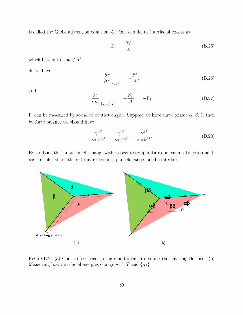
is called the Gibbs adsorption equation [5]. One can define interfacial excess as
Γi ≡Nγi
A(B.25)
which has unit of mol/m2.
So we have∂γ
∂T
∣∣∣∣∣µj
= −Sγ
A, (B.26)
and∂γ
∂µi
∣∣∣∣∣µj 6=i,T
= −Nγi
A= −Γi. (B.27)
Γi can be measured by so-called contact angles. Suppose we have three phases α, β, δ, then
by force balance we should have
γαβ
sin θαβ=
γαδ
sin θαδ=
γβδ
sin θβδ. (B.28)
By studying the contact-angle change with respect to temperature and chemical environment,
we can infer about the entropy excess and particle excess on the interface.
4
dividing surface
(a) 5
(b)
Figure B.2: (a) Consistency needs to be maintained in defining the Dividing Surface. (b)Measuring how interfacial energies change with T and µj
89
We note that in the original definition, Γi depends on the exact location of the dividing
surface (a gauge freedom). In the contact angle experiment, say between α, β, δ, with αβ,
αδ, βδ interfaces, this depth has to be consistent though across different phase boundaries.
In other words, if we retreat the dividing surface location with respect to the actual cαβi (x)
toward the α side, then it has to retreat by the same distance with respect to cαδi (x) toward
the α side as well, otherwise there will be a gap left at the triple junction. Indeed, while inter-
facial excess entropy Sγ/A, excess energy Eγ/A, and excess masses Γi are gauge-dependent,
macro-measurables like the liquid-air surface tensions γαβ, γαδ, γβδ and dihedral angles are
gauge-independent (and this have to do with the fact that when changing the dividing
surface by a few Angstroms, the former atomistic-scale quantities change a lot and can go
from positive to negative, while the numerical value of A will change relatively little, and γ,
which is like a “pressure”-conjugate to A in the free energy, won’t change much with respect
to the definition of the dividing surface).
To remove this uncertainty in the dividing surface location, one can define relative surface
excess:
Γ1i ≡ Γi − Γ1
cαi − cβi
cα1 − cβ1
(B.29)
When there is shift in the dividing surface toward α by ∆, the actual number of atoms
does not change, but the reference state changes, with (cβ1 − cα1 )∆ more type-1 atoms in the
reference state, and (cβi − cαi )∆ more type-i atoms in the reference state, so we will get:
Γ1 → Γ1 + (cαi − cβi )∆, Γi → Γi + (cαi − c
βi )∆, γβδ → γβδ +
C∑i=1
(cαi − cβi )∆µi (B.30)
and it is easy to see that Γ1i is independent of ∆. Type-1 is usually chosen to the solvent
molecule. Alternatively, we can just define the dividing surface so that
Γ1 = 0 (B.31)
so there is no solvent-molecule excess at the interface. When we take a dividing surface so
(B.31) is true, we can directly read off the dividing-surface-independent Γ1i by Γi (which is
dividing-surface-dependent) at that particular dividing surface. This is the dividing surface
we will choose next.
Soap molecules like sodium dodecyl sulfate (SDS) has a hydrophilic head and a fatty hy-
drophobic tail. It dissolves in water, but prefers to segregate to the water-air interface, to
90
reduce the pain of loss of hydrogen bonds, thus
ΓSDS > 0 (B.32)
From the Gibbs adsorption equation, we see that
dγ ≈ −ΓSDSdkBT ln aSDS(aq) (B.33)
where aSDS(aq) is the activity of the SDS molecule solvated in the water, which is close to
the mole fraction when dilute. Then
dγ ≈ −ΓSDSkBT
cSDS(aq)dcSDS(aq). (B.34)
Experimentally, the surface tension of the aqueous phase can be reduced by as much as 70%
from that of plain water. This allows the aqueous solution to wet solids and spread on solid
surfaces more easily. Also, because the soap water has lower surface tension, it delays the
Rayleigh-Plateau instability, and cause soap bubble to be more stable (it also reduces the
rate of water evaporation kinetically).
Also, by varying the temperature or composition spatially, the surface tension γ(T (x),X(x))
can change, and this gradient in γ induces so-called Gibbs-Marangoni flow or convection
of the fluid:
∇γ = −sγ∇T −∑i
Γi∇µi (B.35)
since ∇γ causes direct imbalance of force per length. The first term above is called thermo-
capillary force, while the rest are called chemo-capillary force. Such transient imbalance
imposes a calming effect on the surface wave, which is used by spear fisherman: they throw
grease into the water, and this calm the water (transiently) so they could see inside the ocean.
According to Franklin’s 1774 paper, “not more than a tea spoonful produced an instant calm
over a space of several yards square, . . . , making all that quarter of the pond, perhaps half
an acre, as smooth as a looking-glass.” [20] This effect can be explained by greatly increased
shear-dissipation due to Gibbs-Marangoni flow.[21]
To explain Franklin’s and other experiments, let us define α ≡ oil phase, β ≡ water phase,
α′ ≡ vapor phase, and solutes like SDS can dissolve in β as well as segregate into αβ interface.
Oil phase wets water, meaning:
γβα′> γβα + γαα
′(B.36)
91
So there is an effective reduction of surface energy after the oil wetting. However, with SDS
dissolved in β (soap water), γβα can drop even more, as the polar head of SDS likes water,
and the non-polar tail of SDS likes oil. This further reduced γβα would make it even easier
for water solvent (β phase) to surround oil phase (α phase) under washing conditions. Thus
SDS is a detergent, that helps to remove oil patches on cloth.
When there is a sinusoidal water (β) wave, even when the α phase is very thin, the density of
oil molecules in flat interfacial region and the curved interfacial region will be different. This
difference in oil molecule density will cause ∇µi, and will actuate the chemo-capillary force
gradient in (B.35), which will then drag the oil film and shear the water beneath it. The
sliding and slippage of β beneath α film will induce a much larger dissipation rate than a
bare γαα′
interface would - it is like a moving solid on top of fluid[21] Only about 15% of the
enhanced water wave damping comes directly from reduced surface tension value. In other
words, the gradient in surface tension is more important than the value of surface tension in
this problem.
The above discussions all assume the interfacial excess free energy (if we take (B.12) to
be definition of γ and think∑i µidNi as the “free energy”). What if the excess energy
is a function of inclination angle φ? Consider the following classic problem of optimizing∫dlγ(φ):
F [φ(x)] ≡∫ xf
xidxγ(φ)
cosφ(B.37)
subjected to the constraint that the curve must pass through (xi, yi) and (xf , yf ):
yf − yi =∫ xf
xidy =
∫ xf
xidx
sinφ
cosφ(B.38)
Imagine any arbitrary change φ(x)→ φ(x) + δφ(x) that satisfies the constraint:
0 =∫ xf
xidx
[cosφ
cosφ− sinφ
cos2 φ(− sinφ)
]δφ(x) =
∫ xf
xidxδφ(x)
cos2 φ(B.39)
which will cause
0 =∫ xf
xidx
[γ′(φ)
cosφ+γ(φ) sinφ
cos2 φ
]δφ(x). (B.40)
The above can only be correct, if
γ′(φ)
cosφ+γ(φ) sinφ
cos2 φ=
λ
cos2 φ(B.41)
92
where λ is a position-independent Lagrange multiplier. Therefore, mechanical equilibrium is
achieved only if
γ′(φ) cosφ+ γ(φ) sinφ = λ (B.42)
for all x. Since in this example, the interface is just a line, force equilibrium along a line
suggest λ is exactly this force. γ(φ) sinφ is the traditional line tension, projected in the
y-direction. If γ′(φ) ≡ dγdφ
= 0, then solving (B.42) as an ODE would give us
sinφ(x) =λ
γ→ φ(x) = const (B.43)
e.g. a straight line. But if γ(φ) then generally it will be a curved, or even kinked line. The
γ′(φ) cosφ is easily explained as torque term. So the surface tension is just
t =dγ
dφm + γξ (B.44)
for a 1D line, where ξ is the line direction and m ⊥ ξ.
B.1.1 McLean Isotherm for Interfacial Segregation
The interfacial excess of a solute Γi usually takes a “Fermi-Dirac” shape when µi is varied
(kBT ln γiXi). That is, for very small or very large µi, there is vanishing slope:
dΓid ln γiXi
→ 0 (B.45)
indicating there is a fixed number of sites in the solid interface that is either all empty (“0”)
or all occupied (“1”). Thus there is a peak slope location:
maxdΓi
d ln γiXi
(B.46)
Imagine a dilute 1-2 solid solution in the bulk lattice:
X2 1 (B.47)
and a grain boundary. Suppose the GB has a site density Γ (mole/area, or #/area), forming
93
a monolayer. So at most, we have occupancy:
max Γ2 = Γ (B.48)
(In above, we ignore the dividing plane choice, since X2 is very small in either side of the
interface). We can define interfacial composition to be
Xγ2 ≡
Γ2
Γ. (B.49)
We can also define solute enrichment factor s to be
s ≡ Γ2
ΓX2
=Xγ
2
X2
(B.50)
Suppose these sites are either occupied by 1 or 2, and cannot be vacant (e.g. the energy
penalty is too high, or the barrier is too sluggish since this requires long-range transport).
In other words, we should only consider 1-2 exchanges with the bulk. The equilibrium of
this facile exchange requires:
µγ2 − µγ1 = µ2 − µ1 (B.51)
We model the right-hand side by an ideal solution:
µ2 − µ1 =∂g
∂X2
∣∣∣∣∣T
= a(T ) + kBT lnγ2X2
γ1(1−X2)(B.52)
with γ2 = γ1 = 1. We will model the left hand side by a regular solution. Basically, let us
assume the interfacial site lattice has coordination number Z (Z = 4 if simple cubic, and 6
if close packed), and suppose only NN interaction on the interfacial site layer is important,
then
gγ(Xγ2 ) = Xγ
2 gγ(1)+(1−Xγ
2 )gγ(0)+kBT [Xγ2 lnXγ
2 + (1−Xγ2 ) ln(1−Xγ
2 )]+f excess (B.53)
where
f excess = ZθXγ2 (1−Xγ
2 ) =Z
2× θ × 2Xγ
2 (1−Xγ2 ), (B.54)
in which θ is the excess bonding energy between 1-2:
θ ≡ −ε12 +ε11 + ε22
2. (B.55)
94
where −ε12 is the amount of energy stablization gained by a 1-2 bond, and 2Xγ2 (1−Xγ
2 ) is
the probability that a certain bond is a 1-2 bond in the mean-field approximation.
If θ < 0, then the system prefers to mix in 2D inside the interface layer. If θ > 0, it prefers
to 2D phase separate (inside the interface layer). Then
∂gγ
∂Xγ2
∣∣∣∣∣T
= gγ(1)− gγ(0) + kBT lnXγ
2
1−Xγ2
+ (1− 2Xγ2 )Zθ (B.56)
therefore we get the isotherm:
X2
1−X2
e− b(T )kBT =
Xγ2
1−Xγ2
e−
2ZθXγ2
kBT (B.57)
with
b(T ) ≡ gγ(1)− gγ(0) + Zθ − a(T ) (B.58)
If we define
α ≡ −2Zθ
kBT, w ≡ X2
1−X2
e− b(T )kBT (B.59)
then
lnXγ2 − ln(1−Xγ
2 ) + αXγ2 = lnw (B.60)
so
dXγ2
(1
Xγ2
+1
1−Xγ2
+ α
)= d lnw (B.61)
sodXγ
2
d lnw=
11Xγ
2+ 1
1−Xγ2
+ α. (B.62)
We see from above that indeed when Xγ2 → 0,
dXγ2
d lnw→ 0+ (B.63)
and when Xγ2 → 1,
dXγ2
d lnw→ 0+ (B.64)
which are saturation behaviors. The peak slope is always reached at Xγ2 = 0.5. We see that
if
α > −4 (B.65)
95
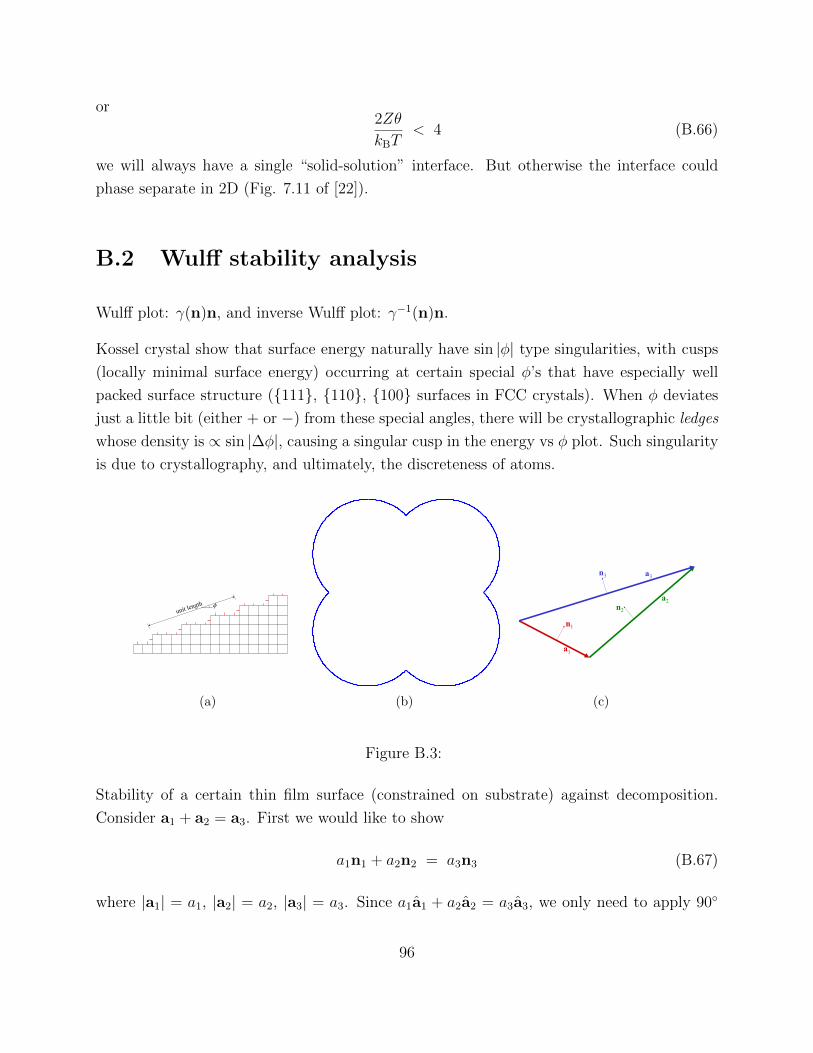
or2Zθ
kBT< 4 (B.66)
we will always have a single “solid-solution” interface. But otherwise the interface could
phase separate in 2D (Fig. 7.11 of [22]).
B.2 Wulff stability analysis
Wulff plot: γ(n)n, and inverse Wulff plot: γ−1(n)n.
Kossel crystal show that surface energy naturally have sin |φ| type singularities, with cusps
(locally minimal surface energy) occurring at certain special φ’s that have especially well
packed surface structure (111, 110, 100 surfaces in FCC crystals). When φ deviates
just a little bit (either + or −) from these special angles, there will be crystallographic ledges
whose density is ∝ sin |∆φ|, causing a singular cusp in the energy vs φ plot. Such singularity
is due to crystallography, and ultimately, the discreteness of atoms.
unit length φ
(a) (b)
n3
n1
n2
a1
a2
a3
(c)
Figure B.3:
Stability of a certain thin film surface (constrained on substrate) against decomposition.
Consider a1 + a2 = a3. First we would like to show
a1n1 + a2n2 = a3n3 (B.67)
where |a1| = a1, |a2| = a2, |a3| = a3. Since a1a1 + a2a2 = a3a3, we only need to apply 90
96
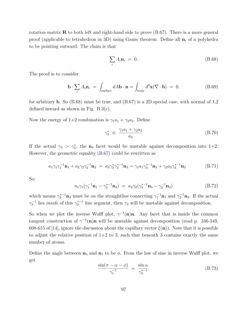
rotation matrix R to both left and right-hand side to prove (B.67). There is a more general
proof (applicable to tetrahedron in 3D) using Gauss theorem. Define all ni of a polyhedra
to be pointing outward. The claim is that
∑i
Aini = 0. (B.68)
The proof is to consider
b ·∑i
Aini =∫
surfacedAb · n =
∫body
d3x(∇ · b) = 0. (B.69)
for arbitrary b. So (B.68) must be true, and (B.67) is a 2D special case, with normal of 1,2
defined inward as shown in Fig. B.3(c).
Now the energy of 1+2 combination is γ1a1 + γ2a2. Define
γ∗3 ≡γ1a1 + γ2a2
a3
(B.70)
If the actual γ3 > γ∗3 , the n3 facet would be unstable against decomposition into 1+2.
However, the geometric equality (B.67) could be rewritten as
a1γ1γ−11 n1 + a2γ2γ
−12 n2 = a3γ
∗3γ∗−13 n3 = γ1a1γ
∗−13 n3 + γ2a2γ
∗−13 n3 (B.71)
So:
a1γ1(γ−11 n1 − γ∗−1
3 n3) = a2γ2(γ∗−13 n3 − γ−1
2 n2) (B.72)
which means γ∗−13 n3 must be on the straightline connecting γ−1
1 n1 and γ−12 n2. If the actual
γ−13 lies inside of this γ∗−1
3 line segment, then γ3 will be unstable against decomposition.
So when we plot the inverse Wulff plot, γ−1(n)n. Any facet that is inside the common
tangent construction of γ−1(n)n will be unstable against decomposition (read p. 346-349,
608-615 of [14], ignore the discussion about the capillary vector ξ(n)). Note that it is possible
to adjust the relative position of 1+2 to 3, such that beneath 3 contains exactly the same
number of atoms.
Define the angle between n3 and n1 to be φ. From the law of sine in inverse Wulff plot, we
getsin(π − α− φ)
γ−11
=sinα
γ∗−13
. (B.73)
97
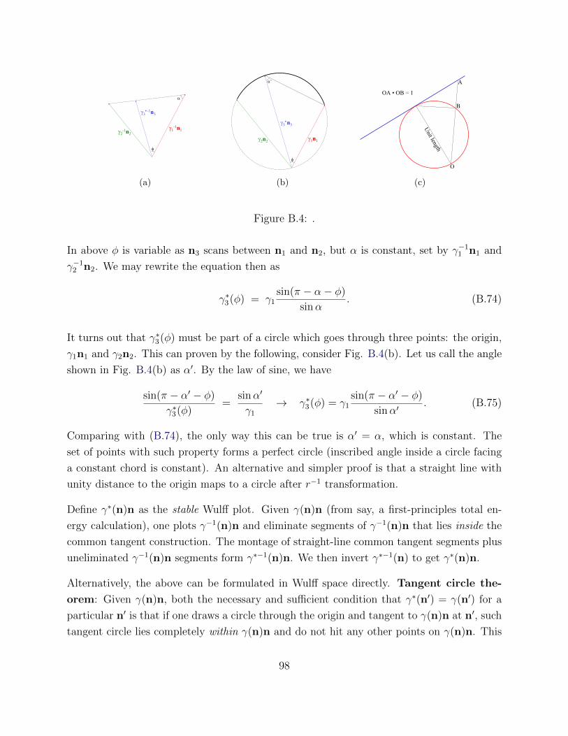
γ3∗-1n3
γ1-1n1γ2-1n2
φ
α
(a)
γ3∗n3
γ1n1γ2n2
φ
α’
(b)
Unit length
O
A
B
OA • OB = 1
(c)
Figure B.4: .
In above φ is variable as n3 scans between n1 and n2, but α is constant, set by γ−11 n1 and
γ−12 n2. We may rewrite the equation then as
γ∗3(φ) = γ1sin(π − α− φ)
sinα. (B.74)
It turns out that γ∗3(φ) must be part of a circle which goes through three points: the origin,
γ1n1 and γ2n2. This can proven by the following, consider Fig. B.4(b). Let us call the angle
shown in Fig. B.4(b) as α′. By the law of sine, we have
sin(π − α′ − φ)
γ∗3(φ)=
sinα′
γ1
→ γ∗3(φ) = γ1sin(π − α′ − φ)
sinα′. (B.75)
Comparing with (B.74), the only way this can be true is α′ = α, which is constant. The
set of points with such property forms a perfect circle (inscribed angle inside a circle facing
a constant chord is constant). An alternative and simpler proof is that a straight line with
unity distance to the origin maps to a circle after r−1 transformation.
Define γ∗(n)n as the stable Wulff plot. Given γ(n)n (from say, a first-principles total en-
ergy calculation), one plots γ−1(n)n and eliminate segments of γ−1(n)n that lies inside the
common tangent construction. The montage of straight-line common tangent segments plus
uneliminated γ−1(n)n segments form γ∗−1(n)n. We then invert γ∗−1(n) to get γ∗(n)n.
Alternatively, the above can be formulated in Wulff space directly. Tangent circle the-
orem: Given γ(n)n, both the necessary and sufficient condition that γ∗(n′) = γ(n′) for a
particular n′ is that if one draws a circle through the origin and tangent to γ(n)n at n′, such
tangent circle lies completely within γ(n)n and do not hit any other points on γ(n)n. This
98
is because a tangent line of γ−1(n)n that does not hit γ−1(n)n at any other point maps to
a tangent circle inside γ(n)n.
The tangent circle theorem and decomposition test is useful for thin-film surface on substrate.
For free-standing crystallite such as formed in deposition, where surface energy dominates the
shape, we need Wulff construction: consider a crystal with f possible surface orientations
ni. Denote their distance to the center as hi. Then the exposed length is ai. Clearly,
ai = ai(hi−1, hi, hi+1). (B.76)
We also have the following reciprocal relation:
∂ai∂hi−1
=∂ai−1
∂hi=
1
sin θi,i−1
, (B.77)
which can be proven from inspecting the geometry, where θi,i−1 is the angle between ni and
ni−1.
Now consider a free-standing particle of fixed volume V . We seek the shape that minimizes
its surface energy:
Fsurface =∑i
γiai, (B.78)
with the shape completely determined by the hi. Change in volume must be constrained
to zero:
0 =∑i
aidhi, (B.79)
and
dFsurface =∑i
(γi−1
∂ai−1
∂hi+ γi
∂ai∂hi
+ γi+1∂ai+1
∂hi
)dhi, (B.80)
so there must be
γi−1∂ai−1
∂hi+ γi
∂ai∂hi
+ γi+1∂ai+1
∂hi= βai, (B.81)
where ai is the Lagrange multiplier. Using the reciprocal relation:
γi−1∂ai∂hi−1
+ γi∂ai∂hi
+ γi+1∂ai∂hi+1
= βai. (B.82)
99
On the other hand, ai(hi−1, hi, hi+1) is a homogeneous function of degree 1 (in 2D):
ai(lhi−1, lhi, lhi+1) = lai(hi−1, hi, hi+1) (B.83)
So by taking derivative against l on both sides, and then setting l = 1, there is
hi−1∂ai∂hi−1
+ hi∂ai∂hi
+ hi+1∂ai∂hi+1
= ai. (B.84)
In 3D, there is ai(lhi−1, lhi, lhi+1) = l2ai(hi−1, hi, hi+1) and hi−1∂ai∂hi−1
+hi∂ai∂hi
+hi+1∂ai∂hi+1
= 2ai.
Comparing the two equations, we see that
... =γi−1
hi−1
=γihi
=γi+1
hi+1
= ... = β (B.85)
for all i, will be a variational extremum. In fact, dFsurface = dFbulk = (Pint − Pext)dV
is the original Young-Laplace pressure argument (Fig. ??(a)), and the facet-independent
Lagrange multiplier β can be identified to be simply the Young-Laplace pressure difference
∆P = Pint − Pext. So in 2D, we have ∆P = γihi
.
The above means that the inner envelope formed by all Wulff planes (a Wulff plane lies
perpendicular to γ(n)n at γ(n)n) gives the equilibrium shape of a free-standing nanocrystal.
This is called Wulff construction, which minimizes the total surface energy of a free-
standing nanoparticle. Note that the Wulff construction serves a different purpose from the
tangent circle theorem. The tangent circle theorem deals with the stability of one surface
constrained to have overall inclination n′ because it must conform to the substrate, whereas
the Wulff construction needs to optimize all facets of the nanocrystal simultaneously.
In 3D, there is an extra factor of 12
on RHS, and we get
... =γi−1
hi−1
=γihi
=γi+1
hi+1
= ... =β
2=
∆P
2(B.86)
or ∆P = 2γihi
to be the pressure increase inside the solid particle. We see that for isotropic
surface energy and spherical particle, this reduces to the familiar expression ∆P = 2γR
.
100
B.3 Gradient Thermodynamics Description of the In-
terface
First-order phase transition is characterized by finite jump in the order parameter ηα → ηβ
as soon as T = T±e (the nucleation rate may be very small, but theoretically suppose one
waits long enough one can witness this finite jump at T±e ). For example, melting of ice
at P = 1atm is a first-order transition because as soon as T rises up to 0.0001C and
melting can occur, there is a finite density change from ice to liquid water, and there is an
obvious change in the viscosity as well. Also spatially, the transition from η(x) = ηα to
η(x′) = ηβ typically occurs over a very narrow region: the shortest distance between x and
x′ (interfacial thickness w) is typically less than 1nm. Previously, we assigned a capillary
energy γ to this interfacial region without discussing this region’s detailed structure. Such
“sharp interface” view, where one ignores the detailed interfacial structure and represent it
as a geometric dividing surface, is sufficient for most first-order phase transition problems.
If one is really interested in the physical thickness of this interfacial region however, one
must use so-called gradient thermodynamics formulation [17] to be introduced below, where
the capillary energy∫γdA in the sharp-interface representation is replaced by a 3D integral
involving a gradient squared term∫K|∇η(x)|2d3x with K > 0. The above replacement
makes sense intuitively, since the interfacial region is characterized by large gradients in
η(x), absent in the homogeneous bulk regions of α or β. Nucleation and growth is a must
for all first-order phase transitions, where large change (ηα → ηβ) occurs in a narrow region
(the interface) even during nucleation.
In contrast, second-order phase transition is characterized by initially infinitesimal changes
over a wide region. These initially infinitesimal changes appear spontaneously in the system
and grow with time, without going through a nucleation (large change in a small region)
stage. For example, in the paramagnetic (α)→ferromagnetic (α1,α2) transition of pure iron
as T is cooled below Tc = 1043K (the Curie temperature, also called the critical point), both
the spin-down α1 and the spin-up α2 phase have very small magnetic moments: ηα1 = −m,
ηα2 = m, with m ∝ (Tc − T )1/2. Microscopically, going from α1 to α2 near Tc would
involve the flipping of a very small number of spins. So the high-temperature paramagnetic
phase, and the two low-temperature ferromagnetic phases are very similar to each other
near Tc: |ηα − ηα1|, |ηα − ηα2| ∝ (Tc − T )1/2, where η is the magnetic moment. The breakup
of a uniform paramagnetic domain into multiple ferromagnetic domains upon a drop in
temperature below Tc is spontaneous and instantaneous and does not require a nucleation
101
stage: it is growth, off the bat. In other words, no under-cooling is required for observing
the start of second-order phase transition within a given observation period. The growth
happens essentially instantaneously at T = T±c . Although, to see the growth and coarsening
to a certain amplitude would require time.
The way a system can accomplish second-order transition vis-a-vis first-order transition is
best illustrated using the binary solution example: gsoln(X2, T ) ≡ Gsoln(N1, N2, T )/(N1+N2).
Suppose Ω1 = Ω2 = Ω, we may define specific volume free energy as
gv(c2) ≡ Ω−1gsoln(X2 = c2Ω) (B.87)
so the bulk solution free energy for a homogeneous system is just
Gsoln =(∫
d3x)gv(c2). (B.88)
gv(c2) is the same function as gsoln(X2) after horizontal and vertical scaling. So the tangent
extrapolation of gv(c2) to c2 = 0 (corresponding to X = p1) would give Ω−1µ1, and tangent
extrapolation of gv(c2) to c2 = Ω−1 (corresponding to X = p2) would give Ω−1µ2. c2(x) is
our order parameter field η(x) here. For an inhomogeneous system, the solution free energy
should intuitively be written as
Gsoln =∫d3xgv(c2(x)). (B.89)
Using the above as reference, the total free energy then looks like:
G =∫d3x(gv(c2(x)) +K|∇c2(x)|2) +Gelastic (B.90)
where the gradient squared term replaces the capillary energy∫γdA. Gelastic = 0 if Ω1 =
Ω2 = Ω. (B.90) is a unified model that can be used to investigate both finite interfacial
thickness in first-order transitions [17], as well as second-order transitions [23]. Since K > 0,
the model (B.90) punishes sharp spatial gradients, the origin of interfacial energy. On the
other hand if all changes occur smoothly over a large wavelength with small spatial gradients,
then G approaches Gsoln. Since Gsoln is the driver of phase transformation (gradient/capillary
and elastic energies are typically positive), let us consider what Gsoln wants to do first.
For a closed system, c2 is conserved:∫d3xc2(x) = const (B.91)
102
which means it is possible to partition the solutes, but it is not possible to change the
total amount of solutes in the entire system. For instance, if one starts out with a uniform
concentration c2(x) = cα2 , a partition may roughly speaking occur as:
cα2 = fα1cα12 + fα2cα2
2 , (B.92)
where volume fraction
fα1 =cα2
2 − cα2cα2
2 − cα12
, fα2 = 1− fα1 =cα2 − cα1
2
cα22 − cα1
2
(B.93)
of the region has c2(x) = cα12 and c2(x) = cα2
2 , respectively, separated by sharp interfaces.
The solution free energy of the partitioned system is then
Gsoln =(∫
d3x)
(fα1gv(cα12 ) + fα2gv(c
α22 )) (B.94)
compared to the unpartitioned and uniform original system (∫d3x) gv(c
α2 ).
Local stability means Gsoln is stable against small perturbations in c2(x). The necessary and
sufficient condition for local stability is that
∂2gv∂c2
2
> 0. (B.95)
If ∂2gv∂c22
< 0, a small partition with cα12 ≈ cα2 ≈ cα2
2 would be able to decrease Gsoln. For
example, with cα22 = cα2 + ∆c, cα1
2 = cα2 −∆c, fα1 = fα2 = 1/2, one has
Gsoln∫d3x
=1
2gv(c
α2 −∆c) +
1
2gv(c
α2 + ∆c) = gv(c
α2 ) +
1
2
∂2gv∂c2
2
(cα2 )(∆c)2 + ... (B.96)
which would be lower than uniform gv(cα2 ) if ∂2gv
∂c22< 0. A sinusoidal perturbation
c2(x) = cα2 + a(t) sin(k · x) (B.97)
would also have equal amount of “ups and downs”, and would thus also reduce Gsoln. The
reason sinusoidal perturbation is preferred (at least initially) compared to the step function
between cα2 − ∆c and cα2 + ∆c is that it minimizes the gradient energy by spreading the
gradients around. Therefore if ∂2gv∂c22
< 0, its amplitude a(t) will increase with time. This is
the trick behind spinodal decomposition, or more generally second-order phase transitions,
103
which can reduce the system free energy without nucleation. Nucleation is not needed here
because the system’s initial state does not have local stability. The loss of local stability is
induced by temperature, i.e.
∂2gv∂c2
2
(cα2 , T+C ) > 0,
∂2gv∂c2
2
(cα2 , T−C ) < 0 (B.98)
thus∂2gv∂c2
2
(cα2 , TC) = 0. (B.99)
During initial growth of the sinusoidal profile in the unstable composition range, the solutes
appears to diffuse up the concentration gradient (Fig. 5.39 of [13]). According to the
phenomenological Fick’s 1st law J2 = −D∇c2, this would mean a negative interdiffusivity
D(c2) < 0. This is in fact not surprising, because D (from D1, D2) contains thermodynamic
factor 1 + d ln γ2d ln c2
, which can be shown to be X2(1−X2)kBT
∂2g∂X2
2and thus have the same sign as
∂2g∂X2
2. When ∂2g
∂X22
is negative, D is negative. This means that at the most fundamental level,
diffusion is driven by the desire to reduce free energy or chemical potential, and not by the
desire to smear out the concentration gradient.
Mathematically, while a positive diffusivity tends to smear out the profile (the shorter the
wavelength, the faster the decay of the Fourier component amplitude), a negative diffusivity
would tend to increase the roughness of the profile. The growth of very-small wavelength
fluctuations in spinodal decomposition will be punished by the gradient energy, though.
Thus an optimal wavelength will be selected initially, which can be tens of nms. Later,
after the compositions have deviated largely from cα2 , the microstructural lengthscale may
further coarsen, although the interfacial lengthscale will sharpen. Because α1 and α2 do not
come out of a nucleation and growth process, but amplification of sinusoidal waves of certain
optimal wavelength, they lead to unique-looking interpenetrating microstructures.
In contrast to spinodal instability, in a first-order phase transition the system’s initial state
has never lost its local stability. At T = T+e , one is in a globally stable uniform composition,
which means
gv(cα2 , T
+e ) < fα1gv(c
α12 , T+
e ) + fα2gv(cα22 , T+
e ) (B.100)
for small and large deviations |cα22 − cα2 | alike (thus a globally stable system must be locally
stable, but not vice versa). Then at T = T−e , c2(x) = cα2 becomes locally stable only, which
means small deviations would still induce the system energy to go up, but large deviations
104
may induce the system energy to go down. Thus, small perturbations like (B.97) would decay
and die, but large enough perturbations may survive. The chance survival of large enough
perturbations/fluctuations in the order-parameter field is just nucleation.
(B.90) can be used to estimate interfacial thickness w in the following manner. Since ∇c2 ∝(cβ2 − cα2 )/w inside the interface, the gradient energy integral scales as K(cβ2 − cα2 )2/w, so the
wider the interface the better for the gradient energy. On the other hand, right at T = Te,
gv(c2) of the first term connects two energy-degenerate states gv(c2 = cβ2 ) = gv(c2 = cα2 ),
with a bump g∗v − gv(cα2 ) in between. The solution free energy first term thus gives an excess
∝ (g∗v − gv(cα2 ))w, that punishes wide interfaces. The best compromised is thus reached at
w ∝ K1/2|cβ2 − cα2 |(g∗v − gv(cα2 ))−1/2, with interfacial energy γ ∝ K1/2|cβ2 − cα2 |(g∗v − gv(cα2 ))1/2.
It turns out that for Te near Tc, |cβ2 − cα2 | ∝ (∆T )1/2, where ∆T = Tc−Te, and g∗v − gv(cα2 ) ∝(∆T )2, so the interfacial width near the critical temperature would diverge as (∆T )−1/2, and
the interfacial energy would vanish as (∆T )3/2 [17].
Science advances greatly when two seemingly different concepts are connected, for instance
the Einstein relation M = D/kBT . Cahn and Hilliard made a similar contribution when they
connected interfacial energy to critical temperature and second-order phase transformation.
Based on the insight that gradient term should be added to thermodynamic field theories
(fundamentally this is because of atomic discreteness), they developed gradient thermody-
namics formalism for chemical solution systems that predict finite interfacial width, interfa-
cial energy, as well as wavelength selection in spinodal decomposition [23], under one unified
framework. The development can in fact be traced back to the work of van der Waals for
single-component systems, using density as order parameter[24]. Another offshoot of this
approach was provided by Ginzburg and Landau in the theory of superconductivity.
Finally, if Ω1 6= Ω2 the 1-rich α1 phase and 2-rich α2 will have different stress-free volumes,
and to accommodate this mismatch coherently would involve finite elastic energy Gelastic >
0. Growth of the sinusoidal concentration wave would require growth of the associated
transformation strain wave. This would delay the onset of the spinodal instability.
105
Appendix C
Neuromorphic equivalent circuit -
Mantao model
Proton-based electrochemical synapses [1, 25] can operate at very short timescale ∼ ns. Its
structure is similar to that of a battery. We may call the hydrogen reservoir (PdHx) region-0,
the electrolyte region-2, and the HyWO3 region-4. The 0/2 interface will be called 1, and
2/4 interface called 3, where charge-transfer reactions happen.
There is a change of chemical identity at interface 1, where
H(0) ↔ H+(2) + e−(0) (C.1)
and at interface 3,
H+(2) + e−(4) ↔ H(4) (C.2)
where the “(4)” means free electron or H (a bound electron+proton pair) inside the HyWO3
phase, and “(0)” means free electron or H inside the metallic PdHx phase.
Equation C.1, C.2, if they are consummated, are called Faradaic current. Note that Faradaic
current always involves a free electron or a free ion crossing the interface. In C.1 reaction
from left to right, a charge-neutral H(0) auto-ionizes, the proton crosses the interface 1,
leaving an orphaned electron e−(0) behind. In C.1 reaction from right to left, the process
reverses and the proton crosses the interface backwards.
It is also possible for the interface 1 to store excess H+(2), and excess e−(0) across the
106
interface of physical width d1, without consummating the reaction C.1 (that is, no H(0) is
added/subtracted in 0). After all, PdHx is metallic and can store excess electrons on its
surface, and the electrolyte can store excess proton in its surface as well, without these two
reacting. This is called non-Faradaic or capacitive current. The non-Faradaic current leads
to equal and opposite charge ±Q1, stored across the interface ravine d1 that are typically a
few Angstroms. The interfacial area is A1, and typically there is relation
dQ1
dV1
≡ C1 ≈A1ε
d1
(C.3)
where V1 is the electrostatic potential drop across the interface 1, and ε = εrε0 is the dielectric
constant, ε0 = 8.8541878128E − 12 Farad/meter is the vacuum permittivity.
When Equation C.1 reaches thermodynamic balance, there is
U eq(0) = U(0) +e
kBTlnaH+(2)
aH(0)
(C.4)
where −eU(0) = EF(0) is the electronic Fermi energy in PdHx, taking the average electro-
static potential inside 2 to be zero. Similarly, when Equation C.2 reaches thermodynamic
balance, there is
U eq(4) = U(4) +e
kBTlnaH+(2)
aH(4)
, (C.5)
where a’s are the thermodynamic activities, that may be taken to be concentration in ideal-
solution approximation. For simplicity, if we assume (a) H+(2) is the only mobile ion in solid
electrolyte 2, and (b) rigorous electroneutrality inside 2, then aH+(2) is identical everywhere
inside 2, and then
V eq ≡ U eq(0)− U eq(4) = V +e
kBTlnaH(4)
aH(0)
≈ V +e
kBTlncH(4)
cH(0)
(C.6)
where cH(4), cH(0) are the concentrations right at the interface.
It is customary to model these interfaces as R1,C1 and R3,C3, where
V1 ≡ V eq1 +R1I
Faradaic1 , V3 ≡ V eq
3 +R3IFaradaic3 (C.7)
IFaradaic1 can follow the Butler–Volmer equation
IFaradaic1 = A1i
01[ee(1−β1)η1/kBT − e−eβ1η1/kBT ] (C.8)
107
and
IFaradaic3 = A3i
03[ee(1−β3)η3/kBT − e−eβ3η1/kBT ] (C.9)
for electronic (voltage) out-of-equilibrium situations, where i01 and i03 are exchange current
densities. Thus,
η1 ≡ V1 − V eq1 = R1A1i
01[ee(1−β1)η1/kBT − e−eβ1η1/kBT ] (C.10)
η3 ≡ V3 − V eq3 = R3A3i
03[ee(1−β3)η3/kBT − e−eβ3η3/kBT ] (C.11)
We see that
R1 →kBT
eA1i01, R3 →
kBT
eA3i03(C.12)
for small η1, η3 25 mV, but they gets exponentially smaller for larger η1, η3 25 mV:
R1 →η1e
e(β1−1)η1/kBT
A1i01, R3 →
η3ee(β3−1)η3/kBT
A3i03. (C.13)
So the systems of equations are:
V ≡ V eq + η = V +e
kBTlncH(4)
cH(0)
+ η (C.14)
η ≡ η1 + η2 + η3, (C.15)
I = C1dη1
dt+ A1i
01[ee(1−β1)η1/kBT − e−eβ1η1/kBT ]
=A2
L2
κ02
sinh(eη2h/2kBTL2)
eh/2kBTL2
= C3dη3
dt+ A3i
03[ee(1−β3)η3/kBT − e−eβ3η3/kBT ] (C.16)
where the middle equality assumes only ionic Ohmic polarization and no no ionic con-
centration polarization for simplicity, κ02 [unit S/m] is the proton conductivity of the solid
electrolyte at zero field, h is the H+(2) one-hop distance in the thickness direction along 2,
and L2 is the thickness of 2. In this we have also assumed the electronic conductivity in 0
(gate) and 4 (source-drain) is always much better than the ionic conductivity in 2, otherwise
the electronic Ohmic loss in 0 and 4 would also need to be added.
108
There are also two PDEs, one in region-0 and one in region-4, with
∂c
∂t=
∂
∂z
(D0
H
∂c
∂z
), z > z0 (C.17)
∂c
∂t=
∂
∂z
(D4
H
∂c
∂z
), z < z4 (C.18)
for the charge-neutral H (a bound electron+proton pair) concentration. There are the flux
boundary conditions:
A1eD0H
∂c
∂z(z0) = A1i
01[ee(1−β1)η1/kBT − e−eβ1η1/kBT ] (C.19)
A3eD4H
∂c
∂z(z4) = A3i
03[ee(1−β3)η3/kBT − e−eβ3η3/kBT ] (C.20)
In Electrochemical impedance spectroscopy (EIS), equation (C.17), (C.18) correspond to the
Warburg impedance element.
The condition that we work in is huge constant voltage pulse η(t = 0+) (on the order of
4Volt), but very very short time duration. Let us take A1 = A2 = A3 = A. At the beginning,
all the η is to drive ionic Ohmic current inside 2:
I(t = 0+) =A
L2
κ02
sinh(eηh/2kBTL2)
eh/2kBTL2
(C.21)
and so
η3(t) ≈ At
C3L2
κ02
sinh(eηh/2kBTL2)
eh/2kBTL2
(C.22)
and so the Faradaic current (when it is still smaller than the non-Faradaic current) goes as
Ai03[ee(1−β3)η3/kBT − e−eβ3η3/kBT ] (C.23)
it is likely that η3(t) will exceed 25mV, and the Faradaic current gets into the exponential
regime:
Ai03ee(1−β3)η3/kBT (C.24)
but in this regime, the time-dependence should be exponential in time, not powerlaw in time.
The powerlaw may come later, but before there is matching
A
L2
κ02
sinh(eη2h/2kBTL2)
eh/2kBTL2
= Ai03ee(1−β3)η3/kBT (C.25)
109
C.1 Variable resistor solution
Standard RC circuit solves the following equation
CdV
dt= −V
R(C.26)
and this gives the well-known τ = RC time constant.
But what happens when R depends on V ? Suppose
R = R0 exp(− VV0
) (C.27)
then instead of a single relaxation time, the system has a spectrum of relaxation times, which
is very very fast when V is large, but slows down appreciably when V is decaying down.
We havedV
dt= −
V exp( VV0
)
R0C(C.28)
we can define dimensionless voltage and time:
v ≡ V
V0
, s ≡ t
R0C(C.29)
thendv
ds= −vev (C.30)
and we are in the v 1 regime.
Suppose at s = 0, we have v = v0 1. Then the relaxation kinetics is
−e−vdv
v= ds (C.31)
or ∫ v
v0−e−vdv
v= s = Ei(−v0)− Ei(−v) (C.32)
where Ei(·) is a special function called exponential integral.
For positive v, there is also
Ei(−v) = −E1(v) (C.33)
110

so alternatively
s = E1(v)− E1(v0) (C.34)
111
Bibliography
[1] XH Yao, K Klyukin, WJ Lu, M Onen, S Ryu, D Kim, N Emond, I Waluyo, A Hunt,
JA del Alamo, J Li, and B Yildiz. Protonic solid-state electrochemical synapse for
physical neural networks. Nat. Commun., 11:3134, 2020.
[2] N Kamaya, K Homma, Y Yamakawa, M Hirayama, R Kanno, M Yonemura,
T Kamiyama, Y Kato, S Hama, K Kawamoto, and A Mitsui. A lithium superionic
conductor. Nat. Mater., 10:682–686, 2011.
[3] John M. Herbert and Marc P. Coons. The hydrated electron. Annual Review of Physical
Chemistry, 68(1):447–472, 2017. PMID: 28375692.
[4] TF Fuller and J Harb. Electrochemical Engineering. Wiley, first edition, 2018.
[5] Claude H.P. Lupis. Chemical thermodynamics of materials. North-Holland, New York,
1983.
[6] AJ Bard and LR Faulkner. Electrochemical Methods: Fundamentals and Applications.
Wiley, second edition, 2000.
[7] JOM Bockris, AKN Reddy, and Gamboa-Aldeco ME. Modern Electrochemistry 2A:
Fundamentals of Electrodics. Springer, second edition, 2000.
[8] L Chen, AN Alshawabkeh, S Hojabri, M Sun, GY Xu, and J Li. A robust flow-through
platform for organic contaminant removal. Cell Rep. Phys. Sci., 2:100296, 2021.
[9] P Bai, J Li, FR Brushett, and MZ Bazant. Transition of lithium growth mechanisms
in liquid electrolytes. Energy Environ. Sci., 9:3221–3229, 2016.
[10] Terrell L. Hill. An Introduction to Statistical Thermodynamics. Dover, New York, 1987.
[11] Donald A. McQuarrie. Statistical Mechanics. Harper & Row, New York, 1976.
112
[12] A. van de Walle and G. Ceder. Automating first-principles phase diagram calculations.
J. Phase Equilib., 23:348–359, 2002.
[13] David A. Porter and Kenneth E. Easterling. Phase transformations in metals and alloys.
Chapman & Hall, London, second edition, 1992.
[14] Robert W. Balluffi, Samuel M. Allen, and W. Craig Carter. Kinetics of Materials.
Wiley, New York, 2005.
[15] W. L. Bragg and E. J. Williams. The effect of thermal agitation on atomic arrangement
in alloys. Proc. R. Soc. Lond. A, 145:699–730, 1934.
[16] W. L. Bragg and E. J. Williams. The effect of thermal agitation on atomic arrangement
in alloys - ii. Proc. R. Soc. Lond. A, 151:0540–0566, 1935.
[17] J. W. Cahn and J. E. Hilliard. Free energy of a nonuniform system .1. interfacial free
energy. J. Chem. Phys., 28:258–267, 1958.
[18] S. M. Allen and J. W. Cahn. Microscopic theory for antiphase boundary motion and
its application to antiphase domain coarsening. Acta Met, 27:1085–1095, 1979.
[19] Mats Hillert. Phase Equilibria, Phase Diagrams and Phase Transformations: Their
Thermodynamic Basis. Cambridge University Press, New York, 1998.
[20] B. Franklin. Of the stilling of waves by means of oil. extracted from sundry letters
between benjamin franklin, ll. d. f. r. s. william brownrigg, m. d. f. r. s. and the reverend
mr. farish. Philosophical Transactions, 64:445–460, 1774.
[21] P Behroozi, K Cordray, W Griffin, and F Behroozi. The calming effect of oil on water.
Am. J. Phys., 75:407–414, 2007.
[22] A.P. Sutton and R.W. Balluffi. Interfaces in crystalline materials. Clarendon Press,
Oxford, first edition, 1995.
[23] J. W. Cahn. On spinodal decomposition. Acta. Met., 9:795–801, 1961.
[24] Johannes Diderik van der Waals. The thermodynamik theory of capillarity under the
hypothesis of a continuous variation of density. Konink. Akad. Weten. Amsterdam, 1:56,
1893.
113
[25] M Onen, N Emond, J Li, B Yildiz, and JA Del Alamo. Cmos-compatible protonic pro-
grammable resistor based on phosphosilicate glass electrolyte for analog deep learning.
Nano Lett., 21:6111–6116, 2021.
114