Keskustelualoitteita #49 Joensuun yliopisto, Taloustieteet

Normative and Descriptive Theories of Decision Making under Risk:

A Short Review

Niko Suhonen

ISBN 978-952-458-985-7 ISSN 1795-7885

no 49

Normative and Descriptive Theories of

Decision Making under Risk:

A Short Review

Niko Suhonen*

Economics and Business Administration University of Joensuu, Finland (niko.suhonen@joensuu.fi)

JUNE 2007

Abstract

The paper discusses some recent developments in analysis of decision making under risk and uncertainty. First we present the expected utility theory and the basic assumptions of rationality. Second we discuss the critique that has been directed towards the expected utility theory. Next we present the alternative theories: regret theory, prospect theory and theory of stochastic preference. Finally we discuss some practical examples from casinos and gambling markets. It is argued that descriptive theories (e.g. prospect theory) have taken room from normative theories (e.g. expected utility theory). We conclude that we should push forward with empirical testing, both experimental and non-experimental, and develop descriptive theories in the future. However normative and descriptive theories are not mutually exclusive. Both are needed in real life decision making.

Keywords: Risk, Uncertainty, Expected Utility Theory, Prospect Theory

* I thank Matti Estola, Mika Linden, Jani Saastamoinen and Timo Tammi for valuable comments and suggestions. Financial support from Yrjö Jahnsson Foundation and Finnish Cultural Foundation is also gratefully acknowledged.

1. Introduction Gambling, risk, bet, and gain. All these words invoke feelings or at least some interest, either

positive or negative. These conceptions play a crucial role in decision making under risk and

uncertainty. Various gambles or lotteries have described the risky choices for a long time. From a

practical point of view issues of uncertainty are commonplace in microeconomics (e.g. insurance,

game theory) as well as in macroeconomics (e.g. life cycle income and consumption, tax policy).

In economics, decision-making under uncertainty has been modeled mathematically during the past

fifty years within the framework of the expected utility theory. However, experimental evidence has

challenged the expected utility theory. Therefore, new theories based on evidence have developed.

Contrary to expectations none of the new theories has replaced the expected utility theory.

The paper proceeds as follow. Section 2 presents the expected utility theory and basic assumptions

of rationality. After that we discuss the critique that has been directed towards the expected utility

theory. In section 4 we present the regret theory, prospect theory, and theory of stochastic

preference. Section 5 includes some findings from real life casino games and betting markets.

Section 6 concludes the review.

2. Expected Utility Theory 2.1 The beginning The Expected Utility Theory (for now on EUT) was first proposed by Daniel Bernoulli (1738).

Bernoulli puzzled over a problem that how much a rational individual is prepared to pay to enter a

gamble? The most common conception was that gamblers could pay expected monetary value of

the gamble but nothing more. However, Bernoulli gave a following counterexample: suppose that

we throw a coin repeatedly until we get heads. Our winning sum is , where n is a number of

throws until we get the first heads. As there is always a non-zero probability that n can be very large

the winning sum can increase infinitely. This is the so-called St. Petersburg gamble or paradox.

Bernoulli drew conclusions that individuals are just preparing to pay a small amount of money for

this type of gambles. In other words, individuals change money bets for some kinds of “utilities”.

n2

John von Neumann and Oskar Morgenstern (1944) considered the same problem and developed the

Expected Utility Theory. This is also called von Neumann-Morgenstern EUT. The main aspects of

EUT are the preferences and the axioms, which determine decisions under risk and uncertainty.

1

Most of these axioms rest on an assumption that individuals are rational and they have well-defined

preferences.

Note that traditional decision theories separate concepts of risk and uncertainty. Decision-making

under risk means that outcome probabilities are known, whereas in decision making under

uncertainty these probabilities are unknown. However, most decisions are made in the middle field

between known and unknown probabilities. Therefore, we do not separate decisions under risk and

uncertainty.

Let be a consequence or an outcome of some action or choice. happens with a probability .

These can be, widely thinking, such as: dead, illness, luck, money etc. However, assume that

consequences are a list of measurable monetary values. So, a set of pure consequences can be

written as

ix ix ip

1( ,..., )nx x x= . These mutually exclusive consequences are associated with the

probability distribution 1( ... )np p p= , where for all and 0≥ip i ∑ =i ip 1 . Now, the consequences

and probabilities together present a vector, which is called a prospect or gamble, and which can be

represented in a form 1 1( , ),...., ( , )n nx p x p=q . Thus, the prospect is to be understood as a list of

consequences with associated probabilities. More generally, only lowercase letters in bold (e.g. q, r,

s) will be used to note prospects.

2.2 Axioms Expected Utility Theory can be derived from three separate axioms: ordering, continuity, and

independence.

1) Ordering. The ordering axiom includes both completeness and transitivity (Starmer 2000).

Completeness entails that for all prospects q, r: either or , where

represents a relation ”is preferred to” (weakly). Respectively, transitivity requires for all r,

q, s: if and , then . In words, transitivity expresses a rational

ordering of preferences.

( )q r≺ ∼ ( )r ≺ ∼ q

r s s

r

( )≺ ∼

( )q ≺ ∼ ( )r ≺ ∼ ( )q ≺ ∼

2) Continuity. Continuity demands that for all prospects r, q, s where and

there must exist some , so that

( )q ≺ ∼ ( ) ,r s≺ ∼

p rsq ~)]1,(),,[( pp − , where ~ express the relation of

indifference.

2

3) Independence. Independence requires that for all prospects r, q, s: if , then

( )q ≺ ∼ r

)]1,)(,[( pp −sq ( )≺ ∼ )]1,(),,[( pp −sr for all p .

Furthermore, EUT usually assumes monotonicity.

4) Monotonicity. Let 1,...., nx x be a list of consequences ordered from the worst to the

best . Then we can say that prospect q´s probability distribution

will first-order stochastically dominate another prospect r´s probability distribution

if for all ,

)( 1x

)( nx ),...,( 1 qnqq ppp =

),...,( 1 rnrr ppp = ix ni ,...,1=

.n n

qj rjj i j i

p p= =

≤∑ ∑

From now on, when we are discussing of individual rationality, we intend that an individual

behaves according to the above axioms and assumptions.

2.3 Expected Utility Preferences over prospects can be represented by function , which gives a real-valued index to

each prospect. Function operates between prospects so that . An

individual will choose prospect q over prospect r if and only if a value of the index q is no less than

a value of the index r. We also assume that an individual maximizes the function index.

(.)V

(.)V ⇔≥ )()( rq VV ( )q ∼ r

Furthermore, the expected utility theory to choices between prospects is based on the following

three tenets.

i) Expectation: If all three axioms ordering, continuity and independence hold,

preferences to prospect q can be represented by

∑ ++=⋅=i nnii xupxupxupV ),(...)()()( 11q

3

where is a utility function. We assume that the utility function is continuous,

monotonous and at least twice differentiable. Thus, is the expected utility of

prospect q.

(.)u

( )V q

ii) Asset Integration: If W is initial sure wealth before gamble, then an individual will

choose gamble g if and only if

( ) ( ) ( )V V W u W= + >g q .

In other words, a prospect is acceptable if the utility resulting from the prospect

including the initial wealth exceeds the utility of initial wealth alone. Thus, EUT

considers risky decisions from a perspective of final states (which include asset

position) rather than just gains or losses.

iii) Utility Functions: The most common utility functions in the EUT are

Concave, , risk averse. )0´´(.)( >u

Linear, , risk neutral. )0´´(.)( =u

Convex, , risk lover. )0´´(.)( <u

In the EUT, we assume that individuals are risk averse. It implies that an agent with a concave

utility function will always prefer a certain amount to any risky prospect with an expected value

equal to .

x

x

2.4 Subjective Expected Utility Theory

Subjective Expected Utility Theory (SEUT) is also called as Bayesian decision theory. A SEUT

was first developed by Savage (1954). Savage received the basic ideas from Ramsey (1931), de

Finet (1937), and von Neumann and Morgenstern (1944).

The EUT axioms and definitions play also an important role in SEUT. However, there are

differences between these theories. The main difference is that in the EUT probabilities are based

on objective verifiable information, whereas in the SEUT a decision maker perceives probabilities

subjectively: an individual evaluates probabilities of consequences a priori with his or her personal

knowledge or beliefs. Thus, subjective and objective conceptions of probabilities can be unequal.

4

Now, the relevant question is that are individual choices or decisions rational if they are based on

beliefs – not on objective information? At this point, we come across the other side of Bayesian

decisions theory: learning of decision makers. Then we consider the posterior influence. In other

words, individual gamblers observe, learn and try to find information when they confront risky

choices. For example, suppose that we ask from an individual about a probability of a toss, when we

flip an unbiased coin. At first, gambler’s a prior estimate of the toss probability is 0.3. However,

the gambler is a rational decision maker and decides to make flip of coin trials before answering. As

the decision maker has flipped the coin long enough, he or she notices that the posterior probability

is nearer 0.5 than 0.3. So, the gambler decides to answer almost surely that the probability of the

toss is 0.5. As we now notice, the difference between concepts of risk and uncertainty is conjoined

in SEUT.

As regards to a utility function, Savage (1954) pointed out that the function must be bounded at

least from above. The reason is simple: if the function was not bounded, the St. Petersburg paradox

would not vanish. Furthermore, Savage (1954) left open a possibility that utility as a function of

wealth may not be concave, at least in some intervals of wealth. The possibility of non-concave

segments of the utility function has been worked out also by Markowitz (1952) and Friedman &

Savage (1948).

3. Criticism of EUT

3.1 Allais Critique We next turn to some of EUT criticism that has been observed. EUT has been under heavy fire

from the early 1950s. Often the criticism has been motivated by experiments, where it has been

noticed that a decision maker’s decisions systematically violate the rationality axioms.

Allais Paradox

Maybe the most famous paradox was presented by Maurice Allais (1952). It can be presented as

follows. First imagine choosing between two prospects: s1 = [(M€, 1)] and r1 = [(5M€, 0.1),

(1M€, 0.89), (0, 0.01)]. The first option (s1) gives one million for sure. The second (r1) gives five

million with a probability 0.1, one million with a probability a 0.89, and nothing with a probability

0.01. After the first decision, with the same logic, you choose between another two prospects: s2 =

[(1M€, 0.11); (0, 0.89)] and r2 = [(5M€, 0.1); (0, 0.9)].

5

Now, because excepted values of these prospects are E[s1] < E[r1] and E[s2] < E[r2], then

according to the EUT formulation, the preference s1 > r1 should entail the preference s2 > r2, and

conversely. However, Allais expected that people might choose s1 in the first choice, because they

become millionaires for sure. Respectively, as the second choice they might opt for r2, because the

probabilities of winning are similar, but the prizes are very different between s2 and r2. Allais’

conclusion was right because the above phenomenon has been noticed in many experiments (e.g.

Kahneman & Tversky 1979).

An intresting episode occurred in 1952, when Savage, who was a strong supporter of the EUT,

participated a test organized by Allais.1 It happened that Savage was one of those people who

chose as Allais expected. When Savage realized that his choices were against the EUT, he wanted

revise his choices. He claimed that he had been mislead and the more cautions reading of the

problem would have been sufficent to avoid the mistake.

The above example is the famous Allais paradox and it is more generally known by the common

consequence effect. Let us consider the paradox more formally (Starmer 2000). Suppose that we

have the prospects and * [( , )( ,1 )]y p c p= −s * [( , ), ( ,1 )]p c p= −r q , where [( , ), (0,1 )]x λ λ= −q and

10 << λ . Furthermore, assume that monetary consequences , and are non-negative such

that

y c x

yx > . It is worth of notice, that the both prospects s* and r* give a consequence c with the

probability . This is the “common consequence”, and the EUT independence axiom implies

that the choice between the prospects s

)1( p−* and r* should be independent on the value of c . However,

in various experiments it has been perceived that is affected by choices such that an individual

chooses s

c* when , and ryc = * when 0=c (e.g. Slovic ja Tversky 1974).

Common Ratio Effect

Another interesting phenomenon is the common ratio effect, which was also discovered by Allais.

Let suppose that we choose between two gambles. The first gamble gives 3000 € with certainty.

The second one gives 4000 € with the probability 0.8 and nothing otherwise. After that, we choose

once more between gambles such that the first one gives 3000 € with the probability 0.25, otherwise

nothing, and the second one gives 4000 € with the probability 0.2, otherwise nothing. The evidence

from experiments suggest that most people select from the first choice the sure winning prize and

from the second one they opt for 4000 €. However, this is inconsistent with EUT.

1 See more by Gollier 2001.

6

The example can be presented more generally (Starmer 2000). Assume, that we have two prospects

and ** [( , ), (0,1 )]y p p= −s ** [( , ), (0,1 )]x p pλ λ= −r , where yx > and 10 << λ . Furthermore,

assume that the ratio of “winning” probabilities (λ ) is a constant. Therefore, according to the EUT,

the value of probability should not influence the preference relation. To see why, consider any

pair of options {s

p

1* *, r1

* *} where . Next we define a pair of {s1pp = 2* *, r2

* *}, which is similar,

except that the probability is lower than earlier, 2 1p p p= < . Thus, we must have some α

)01( >> α , for which 12 pp α= . As a result, we can now write it as 2 1** [( **, ), (0,1 )]α α= −s s

and 2 1** [( **, ), (0,1 )]α α=r r − , where it follows that choices between such pairs of prospects

should not depend on the value of p . However, there are numerous studies, which make it clear

that people switch their choices from s** to r**, when probability p falls (e.g. Loomes ja Sugden

1987).

Other Problems and Paradoxes

During the last 50 years, other paradoxes have been found as well. One of these is a phenomenon

called preference reversal. This was reported first by Lichentestein and Slovic (1971). They showed

that decision maker’s behavior was not consistent when choices were presented in monetary values.

In other words, the order of choices and monetary values of the choices were inconsistent with each

other. Another paradox is called the Ellsberg paradox (Ellsberg 1961). Ellsberg showed that

decision makers could be influenced by extra information so that they change their preferences from

the certain case to the uncertain without change in probabilities or in winning prizes. For more

details of these problems and others, see for example Camerer (1995), Hargreaves et al (1992) and

Gärdengors & Sahlin (1988).

3.2 Apologia for EUT Based on empirical experiments, many new decision theories have emerged. Consequently, the new

theories have challenged the EUT. Do people really behave as EUT predicts, or can we explain non-

rational behavior by psychological aspects such as fear, enjoyment, disappointment, etc.? The EUT

has been defended from the critique. It has been argued that learning takes place in the real market

environment that does not occur in experiments. On the other hand, the learning process can be

interesting itself (see more by Binmore 1999).

7

However, regardless of critique, we can refer to the methodology of Lakatos. Since none of these

alternative theories can explain all paradoxes, and because none of them is clearly better than the

EUT in general, we cannot refute the EUT (Hausman 1992). On the other hand, it would not be

reasonable to refute all alternative theories either. For that reason, many economists think that we

have one core theory, in this case the EUT, surrounded by alternative theories (e.g. prospect

theory), which can explain exceptional phenomena conflicting the EUT point of view (e.g. Plott

1995). Therefore, economists have tried to separate decision theories in different categories. Next,

we present one alternative.

Normative Theories

Purpose of the normative theories is to express, how people should behave when they are

confronting risky decisions. Thus the behavioral models based on EUT stresses the rationality of

decisions. We are not interested so much on how people behave in real life or in empirical

experiments. Notice that one of these theories is the SEUT. Furthermore, the EUT can be also

defended on grounds that it works satisfactory in many cases.

Descriptive Theories

From the descriptive point of view, we are concerned with how people make decisions (rational and

not rational) in real life. The starting point for these theories has been in empirical experiments,

where it has been shown that people’s behavior is inconsistent with the normative theories. These

theories are, for example, prospect theory and regret theory. We will present some of them more

precisely in the next sections.

Prescriptive Point of View

Prescriptive thinking in risky decisions means that our purpose is to help people to make good and

better decisions. In short, the aim is to give some practical aid with choices to the people, who are

less rational, but nevertheless aspire to rationality. This “category” includes, for example, operation

research and management science.

4. Descriptive Models 4.1 Background New descriptive theories have tried to explain paradoxes and decision problems. Perhaps best-

known theories are the regret theory and the prospect theory. However, there are also several other

8

theories, for example, weighted utility theory (Chew & MacCrimmon 1979), and generalized

expected utility theory (Machina 1982). Most of these theories have the following common features

(Starmer 2000):

i) preferences are represented by some function that is defined over prospects, (.)V

ii) the function satisfies ordering and continuity; and

iii) while is designed to permit observed violations of the independence axiom, the (.)V

principle of monotonicity is retained.

4.2 Regret Theory The descriptive regret theory omits the assumption of preferences transitivity. The theory was

proposed simultaneously by Bell (1982), Fishburn (1982) and Loomes & Sugden (1982,1987). We

discuss the version of Loomes & Sugden (1987). When omitting the transitive preferences, one can

ask, if people can maximize or minimize anything? It turns out that the answer is yes.

The central idea behind the theory is that, when making decisions individuals take into account not

only the consequences that they might get as a result of the action chosen, but also how each

consequence compares with what they would have experienced under the same state of the world,

had they chosen differently. So, the consequences are not independent from each other, and it is

possible that choices are in contradiction with the transitivity assumption. However, people

maximize utility in a sense that they aspire to avoid regret or disappointment.

For example, suppose an individual who is gambling and buying insurance simultaneously. Thus, if

an individual is globally risk averse or risk lover, the behavior is inconsistent with the EUT. The

regret theory explains phenomenon in the following manner. Individuals buy insurance, because

they think that if they do not buy, the situation is bad in case of an accident. Respectively,

individuals also regret, if they would not gamble for a small amount, because in case of winning,

they might “lose” a huge winning prize.

Let us consider regret theory more formally. At first, let the consequence of the ith action ( )

under the jth state of the world ( ) be , and let the probability that the jth state will occur be

. Assume that we have a utility function which assigns to each a basic utility, denoted

by , which represents a degree of pleasure/pain that would be associated with if it was

iA

jS ijx

jp (.)C ijx

ijc ijx

9

experienced under conditions of certainty. Suppose that an individual confronts a choice between

actions and . Furthermore, an individual chooses and then world state occurs. Then

the overall level of satisfaction derived is a combination of the basic utility from the consequence

actually experienced and a decrement or increment of utility due to ´regret´ if or ´rejoicing´

if . Moreover, the overall level of satisfaction, or modified utility, is represented by

where is a regret/rejoice function. For now, the theory can be expressed more

compactly by defining function

iA kA iA jS

ksij cc <

ksij cc >

),( kjijij ccRc + (.,.)R

(.,.)Ψ

),(),(),( ijkjjkikkjijkjij ccRccRccxx −+−=Ψ .

),( kjij xxΨ represents the modified utility of experiencing and missing , minus the modified

utility of experiencing and missing . Loomes and Sugden suggest that individuals choose to

maximise the mathematical expectation of the modified utility. So, preferences between and

are then determined by

ijx kjx

kjx ijx

iA kA

.0~),(~1

≺≺

kjij

n

jjki xxpAA Ψ⇔ ∑

=

In conclusion, regret theory is based on comparison between ´what is´ and ´what might have been´.

Regret theory has explained several but not all paradoxes in EUT.

4.3 Prospect Theory 4.3.1 Discoveries from Experiments

Prospect theory or cumulative prospect theory was formulated first by Daniel Kahneman & Amos

Tversky (1979, 1992). They approached decision making under risk from the point of view of

traditional behavioural sciences. Kahneman (1992) even argued that people not necessarily try to

maximize their utility. Findings, which Kahneman & Tversky (1979, 1981, 1986) have made in

their experiments, are the groundwork for prospect theory. They answer to the discussed paradoxes

and problems in EUT.

Certainty effect. Kahneman and Tversky called the result of the Allais paradox (see above) as the

certainty effect. It means that people tend to choose a sure gain when it is possible.

10

Reflection effect. The Allais paradox is converse when consequences are negative. People’s risk

aversion changes to risk seeking in a case of negatives outcomes. In other words, an individual’s

utility function is concave for winnings and convex for losses.

Framing effect. The EUT assumes that individual decision-making is invariant to the manner of

representation. However, there is much evidence that variation in the framing of options (e.g. gains

or losses) yields systematically different preference relations.

Isolation effect. Isolation effect, in general, means that decision makers are more interested in

absolute changes of wealth than final asset position that includes current wealth. Kahneman and

Tversky (1979) made an experiment, where individuals were provided before a risky decision a sure

amount of money. However, this did not influence their decisions. This is inconsistent with the

assumption of asset integration in the EUT.

Probabilistic insurance. Consider an example as follow. A person is offered insurance, which

covers all the losses on alternate days. Respectively, the insurance does not cover the losses during

the every second day. Moreover, the price of the insurance is half of full insurance. By the evidence

from experiments, Kahneman and Tversky noticed that people are not willing to accept or buy the

insurance of this type In the EUT point of view, if the full or regular insurance is not offered

decision makers should accept probabilistic insurance.

4.3.2 Probability Weighting Function

In the previous section, we considered the SEUT. It was based on the concept of a subjective

probability, where we assumed that individuals have a prior probability weighting on outcomes. A

probability weighting function differ from the subjective probability. The function can be clarified

as follows: an individual changes probabilities, which can be objective, to his or her beliefs that are

based on real probabilities. Let the probability weighting function be , which gives a

weighted value for probability . Furthermore, assume that is increasing with

( )iw p

ip ( )iw p (0) 0w = and

. So, we can write a simple extended variant of this type of model, where an individual is

assumed to maximize the decision-weighted function

(1) 1w =

. (1) ∑ ⋅=i ii xupwV )()()(q

11

Kahneman and Tversky (1979) used first time the equation to model prospect theory.

Unfortunately, the model violates stochastic dominance (see more, Prelec 1998). However, the

rank-dependent representation, first developed by Quiggin (1982), avoids the problem of stochastic

dominance. Moreover, Kahneman and Tversky (1992) used latest version, called cumulative

prospect theory, or a cumulative weighting function, which was consistent with the stochastic

dominance and which can differ for gains and losses. We will examine the weighting function in

later section.

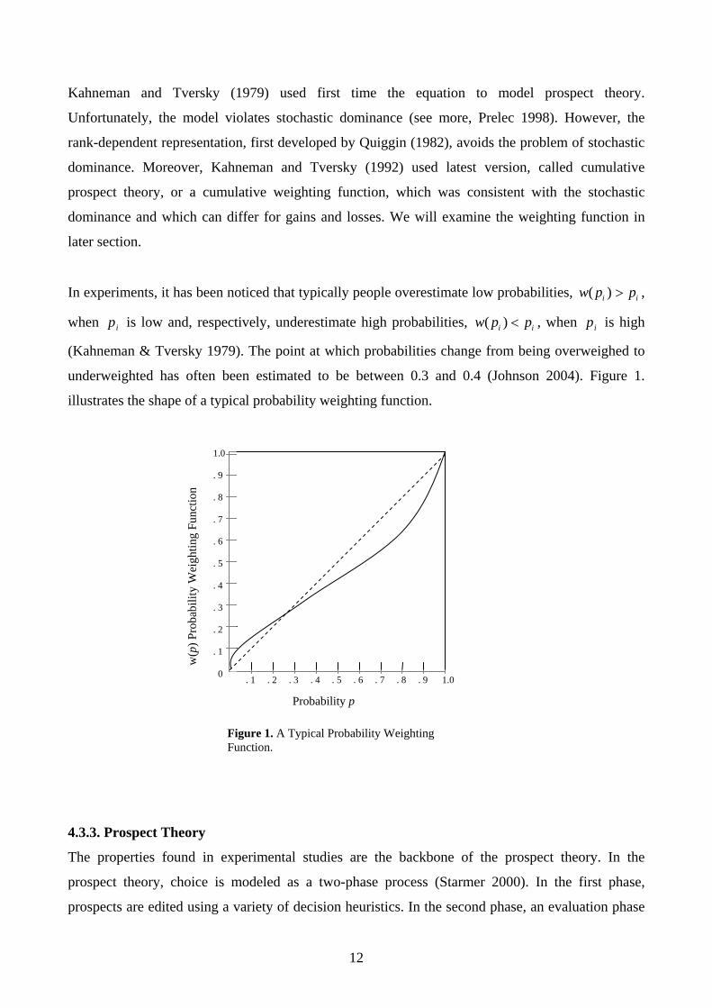
In experiments, it has been noticed that typically people overestimate low probabilities, ,

when is low and, respectively, underestimate high probabilities, , when is high

(Kahneman & Tversky 1979). The point at which probabilities change from being overweighed to

underweighted has often been estimated to be between 0.3 and 0.4 (Johnson 2004). Figure 1.

illustrates the shape of a typical probability weighting function.

( )i iw p p>

ip ( )iw p p< i ip

1.0 . 9 . 8 . 7 . 6 . 5 . 4 . 3 . 2 . 1 0 . 1 . 2 . 3 . 4 . 5 . 6 . 7 . 8 . 9 1.0

w(p

) Pro

babi

lity

Wei

ghtin

g Fu

nctio

n

Probability p

Figure 1. A Typical Probability Weighting Function.

4.3.3. Prospect Theory

The properties found in experimental studies are the backbone of the prospect theory. In the

prospect theory, choice is modeled as a two-phase process (Starmer 2000). In the first phase,

prospects are edited using a variety of decision heuristics. In the second phase, an evaluation phase

12

of choices over edited prospects is determined by a preference function, which can be presented by

the decision-weighted utility function defined above (Eq.1). However, Kahneman and Tversky´s

(1992) later version of prospect theory has no formal editing phase, although, they do mention that

editing may be important.

Editing routines in prospect theory are essentially rules for simplifying prospects and transforming

them into a form that can be easily handled in the second phase. Major operations of the editing

phase are

i) Coding. The evidence discussed in the previous section shows that individuals normally

perceive consequences as gains and losses, rather than as final states of wealth or

welfare. So, the gains or losses are defined relative to some neutral reference point.

Kahneman and Tversky argue that the reference point will typically be the current asset

position.

ii) Combination. Combination is an operation which simplifies prospects by combining the

probabilities associated with identical outcomes. For example, a prospect described as

may be evaluated as a simplified prospect like

. Notice, that these two prospects are not equivalent in general,

if the weighting function is nonlinear.

),...],(),,(),,[( 332111 pxpxpx

),...],(),([( 33211 pxppx +

iii) Segregation. Segregation involves separating risky from less risky components of the

prospect. For example, if outcomes and are both positive and x y yx < , then prospect

[( , ), ( ,1 )]x p y p− can be separated to two prospects and . ),( px )1,( pxy −−

iv) Cancellation. The operation of cancellation involves discarding the components of

choices that are common to all prospects. Thus, a choice between prospects

and )]1,(),,[( ppx −= qs´ ´ [( , ), ( ,1 )]x p p= −r r can be evaluated directly between the

prospects q and r.

As previously discussed, Kahneman and Tversky (1992) do not represent the editing phase formally

in their later model. The reason for this is that they used a rank-dependent probability weighting

model. It explains many of editing phase procedures, but not all, such as framing effect. However,

13

we can generally assume that in the evaluation phase, the decision-maker evaluates the prospects

that are attainable to him or her after the conclusion of the editing phase. Thus, in the evaluation

phase, the prospect’s value is expressed by a value function , which operates in a similar way

as in the EUT and the decision-maker chooses the prospect with the highest value. Moreover, two

scales determine the value function: first, cumulative or rank-dependent probability weighting

functions and , which determine different weights to probabilities of losses and gains,

and second, the utility function

(.)V

+(.)w −(.)w2 that assigns utilities to outcomes. Notice, that the utility

function is defined on deviations from the reference point. Let us consider more precisely the value

function .

(.)v

(.)V

In the prospect theory there are two types of prospects: simple prospects with one nonzero outcome,

, and binary prospects with nonzero outcomes ),( px=q [( , ), ( , )]x p y q=q , where q also represents

a probability. Moreover, we can now represent preferences by the following formulas (Prelec 1998)

(2) ⎪⎩

⎪⎨⎧

<

>=

−

+

.0),()(,0),()(

),(xxvpwxxvpw

pxV

( ) ( ) ( )( ( ) ( )), 0 , (3.1)

[( , ), ( , )] ( ) ( ) ( )( ( ) ( )), 0, (3.2)( ) ( ) ( ) ( ), 0 . (3.3)

w p q v x w q v y v x x yV x p y q w p q v x w q v y v x y x

w p v x w q v y x y

+ +

− −

− +

⎧ + + − < <⎪

= + + − < <⎨⎪ + < <⎩

Equation 2 is simple, non cumulative. Equations 3.1 and 3.2 are cumulative. So, if and x y have

the opposite signs, as in Eq. 3.3, then the prospect is framed as losing an outcome with a

probability and gaining an outcome with a probability . On the other hand, if both and

are gains (Eq. 3.1), or if both are losses (Eq. 3.2), then the prospect

x

p y q x y

[( , ), ( , )]x p y q=q is framed as a

chance of gaining (losing) at least the value of middle outcome , and a chance of

gaining (losing) an extra . To summarize this, the argument of the weighting function is

the cumulated probability of an outcome at least good as , if is positive, or at least as bad as

, if is negative. The intuition of the result is the same as segregation in editing phase (see

above).

´´ qp + )(xv ´´q

)()( xvyv −

x x

x x

2 Kahneman and Tversky used term “value function”. However we proceed by using term “utility function” in order to clarify the concepts.

14

As a result, Kahneman and Tversky proposed that the prospect theory utility function has three

main characteristics:

1) Defined on deviations from the reference point,

2) Concave for gains and convex for losses, and

3) Steeper in the domain of losses.

Utility

Losses Gains

Figure 2. The Valuation of Outcomes in Prospect Theory

Kahneman and Tversky assumed that is concave above the reference point and convex below

it. These properties reflect the principle of diminishing sensitivity. So, the impact of a marginal

change will decrease as we move further away from the reference point. For example, relative to the

reference point the difference between gain of 10 € and 20 € will seem larger than the difference

between gains of 110 € and 120 €. More generally, Kahneman and Tversky assumed diminishing

marginal utility for gains ( , when ) and diminishing marginal disutility for losses

( , when ). Moreover, they assumed that is steeper for the losses than for the

gains. This is a principle of loss aversion, which implies that losses loom larger than corresponding

gains. Loss aversion is modelled by imposing the condition

(.)v

0)´´( ≤xv 0>x

0)´´( ≥xv 0<x (.)v

)´()´( xvxv −< . Figure 2 illustrates these

properties.

More formally, the weighting function was modelled as a one-parameter function

γγγ

γ

/1))1(()(

ppppw−+

= ,

15

where γ was a shape parameter (see Figure 1.)3. Respectively, the utility function was presented

by a two-part power function

0,

( )( ) 0,

x when xv x

x when x

α

αλ

⎧ ≥⎪= ⎨− − <⎪⎩

where λ indicates loss aversion and α is a shape parameter of utility. Kahneman and Tversky

(1992) estimated values of the parameters. The median exponent of the value function was 0.88 for

both losses and gains, in accord with diminishing sensitivity. The median λ was 2.25 (loss

aversion). The median value of γ for gains was 0.61 and for losses it was 0.69.

We presented previously as an example an individual, who buys insurance and gambles

simultaneously. The prospect theory explains such behaviour by that an individual over weights low

probabilities and underweight high probabilities. So, the simultaneous gambling and buying

insurance is not contradiction.

4.3.4 Prospect Theory and Empirical Evidence

The prospect theory has been tested in many empirical environments. For instance, an individual’s

behaviour in some cases in stock markets is explained by the prospect theory: stock returns react

strongly to positive earnings surprises, but a negative earnings surprise has no significant impact on

returns. The result implies the presence of investor loss aversion where they are reluctant to realize

their losses (see e.g. Ding, D. K. et al 2004). Furthermore, a study from the gambling markets (e.g.

horse race) shows that the prospect theory has a higher explanatory power than the EUT or the

rank-dependent utility theory (e.g. Jullien & Salanié 2000). On the other hand, Bradley (2003)

found evidence that although the gamblers perceive gains and losses rather than final states as

outcomes they were risk loving for gains and risk averse for losses. Moreover, Levy & Levy (2002)

did an experiment, where they found support for the utility function that was exactly the opposite to

the one suggested by the prospect theory.

3 Function form was same for gains and losses, but the value of shape parameter was different.

16

4.4. Theory of Stochastic Preference Finally we present shortly a quite recent descriptive alternative called the theory of stochastic

preference. The theory approaches people’s risky decisions by stochastic valuations. The new

direction has given power to develop new models, test the existing theories, and re-evaluate the

evidence from experiments. A typical experiment shows that some of the EUT axioms contradict

empirical results. The theory of stochastic preferences considers the result as explainable by

stochastic preferences.

First models were proposed by Hey & Orme (1994), Harless & Camerer (1994) and Loomes &

Sugden (1995). Common to all these is that they are based on alternative (deterministic) “core”

theories of preference such as the EUT or some non-expected utility theory. However, the

interpretation of the source of randomness differs between the models. For example, consider the

model by Hey and Orme (1994). Assume that an individual chooses between two prospect q and r.

We can write (Starmer 2000)

[ ] ε+−= )()( rq VVHO ,

where is a preference function of the deterministic core theory and (.)V ε is a stochastic part. If

0=ε , preferences are defined by the core theory. However, if HO is positive, an individual choose

prospect q and conversely. Hey and Orme (1994) assumed that ε is of a normal variety with a

mean of zero. So, the randomness is calculation or measurement error of some type. Notice that if

the difference between the preference functions is high then the probability of prospect change is

low. Respectively, if the difference is low, the probability is high.

5. Examples: Betting markets and Casino Games 5.1 Gambling and Theories What the alternative or non-expected utility theories really offer to economics? Are they nothing

else but gratuitous complications? Note that the EUT can delimit a number of problems out of our

interest in sensible way. Suppose for instance gambling markets. From the EUT point of view it is

not rational that a risk aversive person participates in gambles, where the expected return is

negative, or even zero. Nevertheless, many of us gamble regularly, so something is missing from

EUT. Thus gambling and gambling markets are interesting, because it is an authentic environment

and the evidence from these markets can be used to analyze and test decision-making theories.

Furthermore, if we assume that people behave similarly in other markets as they do in gambling

17

markets, we can use gambling information in other economic fields such as insurance or

investments markets. Next we consider some behavior biases discovered in gambling markets that

are difficult to handle by the EUT.

5.2 Behavior in Horse Races, Casinos, and elsewhere In parimutuel betting in horse races, there is a pronounced bias toward betting on “long shots”,

which are horses with a relatively small chance of winning (see Thaler & Ziemba 1988, Hausch &

Ziemba 1995). More general phenomena are known by the favourite-long shot bias. Over betting

long shots implies that favourites are under bet4. The prospect theory explains this kind of behaving

by the weighting function: gambler over weights low probabilities and under weights high

probabilities.

A second bias is Monte Carlo or a gambler’s fallacy. Put it simple, the gambler’s fallacy is a belief

in negative autocorrelation of a non-autocorrelated random sequence. For example, we throw

repeatedly fair coin. After three heads, we believe that next throw will be tail with a probability

more than 0.5. This bias can be founded for instance in casinos. In many casinos, they have

electronic displays beside the roulette table that show the previous outcomes of the wheel. Many

gamblers make their choices based on the electronic display “information”. However, a roulette

wheel does not have “a memory”. So, consecutive numbers in game are independent of each other

and the likelihood of every number is the same in the next turn.

One interesting related case is the belief bias in mean reverting of game. Typically individual

behaviour is irrational in random walk type games when individuals are far below the “average”

return. In that case, the individual believes that the gamble has “a memory” that “corrects” the

random sequence towards the average in the short run and he/she continues the gaming. The

situation is not explained by normative theories. However, the descriptive prospect theory makes it

possible to model this type of gambling situations. Therefore, we can think that gamblers are

consumers who accept expected losses but behave irrationally if a streak of losses is long enough.

This irrational behaviour can lead to overconfidence to winning chances (Suhonen 2005).

Moreover, it is possible that the behaviour is connected to gambling addiction.

4 Indeed, people dislike favourites so much that if one makes favourite bets it is possible to earn small profit (even accounting for the bookmakers take out rate).

18

6. Conclusion The paper discussed decision making under risk and uncertainty in economics. By force of

experimental economics, the descriptive theories have taken room from the normative theories. The

alternative theories give more arguments to economists when they give policy recommendations.

However, because different theories can give converse recommendations, it is problematic to know

which theory is the best one in different situations. Much more empirical research, both

experimental and non-experimental, is needed here. In future, the neuroeconomics may help in

some cases (see a short review by Halko 2006). Furthermore, the problem of the descriptive

theories is that they are difficult to enforce in practise. Imagine for instance the prospect theory’s

two-phase decision-making in real life situations such as insurance or stock markets.

The concepts of ´rational´ and ´utility´ are philosophical and multidimensional. Therefore, in my

view, it is dangerous to face and advise individuals only with normative theories. In real life there

are several situations where individuals behave against the EUT axioms but they try to maximize

their utility (e.g. gambling and extreme sports) anyway. The descriptive theories give information

on individual’s biased behaviour and this information can be used as prescriptive support in

economic situations and, more generally, in every real-life risky decisions. Thus, normative and

descriptive theories are not mutually exclusive. They are more like complementary to each other.

References Allais, M. (1953), “Le Comportement de l’Homme Rationnel devant le Risque: Criticue des Postulats et Axiomes de l’Ecole Americaine”, Econometrica 21: 503 – 546. Bell, D.E. (1982), “Regret in Decision Making under Uncertainty”, Operations Research 20: 961-981. Bernoulli, D. (1738, original) (1954),”Exposition on a New Theory on the Measurement of Risk”, Econometrica 22: 23 – 36. Binmore, K. (1999), “Why Experiment in Economics?”, The Economic Journal 109: 16-24. Bradley, I. (2003), “The representative bettor, bet size, and prospect theory”, Economics Letters 78: 409 – 413.

19

Camerer, C. (1995), “Individual Decision Making”, in Kagel, J. H. & A. E. Roth (ed.), The Handbook of Experimental Economics, Princeton University Press, Princeton: 587 – 673.. Chew, S. H. & K. MacCrimmon (1979),”Alpha-nu Choice Theory; a Generalisation of Expected Utility Theory”, Working paper 669, University of British Columbia Faculty of Commerce and Business Administration. de Finetti, B. (1937/1980), “Its logical laws, its subjective sources” in (ed.) H. E. Kyburg, Jr. & H. Smokler, Studies in Subjective Probability, John Wiley, New York: 53 – 118. Ding, D. K. & C. Charoenwong & R. Seetoh (2004), “Prospect theory, analyst forecast, and stock returns”, Journal of Multinational Financial Management 14: 425 – 442. Ellsberg, D. (1961), “Risk ambiguity, and the Savage axioms”, Quarterly Journal of Economics 75: 643 – 669. Fishburn, P. C. (1982), “Nontransitive measurable utility”, Journal of Mathematical Psychology 26: 31 – 67. Friedman, M. & L. J. Savage (1948), “The utility analysis of choices involving risks”, Journal of Political Economy 56, s. 279 – 304. Gollier, C. (2001), The Economics of Risk and Time. The MIT Press, USA. Gärdenfors P. & N-E. Sahlin (ed.) (1988), Decision, Probability, and Utility. Cambridge University Press, USA. Halko, M-L. (2006), ”Mullistaako neurotaloustiede valintateorian?” (in Finnish), Kansantaloustieteen aikakausikirja 103(1): 5-20. Harless, D. W. & C. F. Camerer (1994), “The Predictive Utility of Generalized Expected Utility Theories”, Econometrica 62: 1251 – 1289. Hargreaves H. & M. Hollis & B. Lyons & R. Sugden & A. Weale (1992), The Theory of Choice. Blackwell, Oxford. Hausch, D.B. & W. Ziemba (1995), “Efficiency in sports and lottery betting markets”, in R.A. Jarrow & V. Maksimovic & W.T. Ziemba (ed.), Handbook of finance, Amsterdam. Hausman, D. M. (1992), The inexact and separate science of economics. Cambridge University Press, Cambridge. Hey, J. D. & C. Orme (1994), “Investigating Generalizations of Expected Utility Theory Using Experimental Data”, Econometrica 62: 1291 – 1326. Johnson, E. J. (2004), “Rediscovering Risk”, Journal of Public Policy & Marketing, 23: 2. Jullien, B. & B. Salanié (2000), “Estimating preferences under risk: the case on racetrack bettors”, Journal of Political Economy 108: 503 – 530.

20

Kahneman, D. & A. Tversky (1979), “Prospect Theory: An Analysis of Decision under Risk”, Econometrica 47: 263 – 291. Kahneman, D. & A. Tversky (1992), “Cumulative Prospect Theory: An Analysis of Decision under Uncertainty”, Journal of Risk and Uncertainty 5: 297 – 323. Levy, M. & H. Levy (2002), “Prospect Theory: Much Ado About Nothing?” Management Science 48: 1334 – 1349. Lichtenstein, S. & P. Slovic (1971), “Reversals of Preference between Bids and Choices in Gambling Decisions”, Journal of Experimental Psychology 89: 46 – 55. Loomes, G. & R. Sugden (1982), “Regret Theory; An Alternative Theory of Rational Choice under Uncertainty”, The Economic Journal 92: 805 – 824. Loomes, G. & R. Sugden (1987), “Some Implications of a More General Form of Regret Theory”, Journal of Economic Theory 41: 270 – 283. Loomes, G. & R. Sugden (1995), “Incorporating a Stochastic Element into Decision Theories”, European Economic Review 39: 641 – 648. Machina, M. J. (1982), “Expected Utility Theory without the Independence Axiom”, Econometrica 50: 277 – 323. Markowitz, H. (1952), “The Utility of Wealth”, Journal of Political Economy 60, s. 151 – 158. Neumann, J. v. & O. Morgenstern (1944), The Theory of Games and Economic Behaviour. Princeton University Press, Princeton. Plott, C. R. (1995): Comment to the article: Daniel Kahneman (1994) New Challenges to the Rationality Assumption in Arrow, K. J. & E. Colombatto & M. Perlman & C. Schmidt (ed.) (1996). The Rational Foundations of Economic Behaviour, Macmillan, Hampshire: 220 – 224. Prelec, D (1998), “The probability weighting function” Econometrica 60, s. 497 – 528. Quiggin, J. (1982), “A Theory of Anticipated Utility”, Journal of Economic Behavior and Organization 3:4, s. 323 – 343. Ramsey, F. P. (1931), “Truth and Probability” inBraithwaite R. B. (ed.) The Foundation of Mathematics and Other Logical Esseys Routledge, London: 156 – 198. Savage, L. J. (1954), The Foundations of Statistics. John Wiley, New York. Starmer, C. (2000), “Developments in Non-Expected Utility Theory: The Hunt for a Descriptive Theory of Choice under Risk”, Journal of Economic Literature 38: 332 – 382. Suhonen, Niko (2005), ”Riskinalaiset päätökset toistuvissa pelitilanteissa: Rahapelit ja subjektiivisuus”(in Finnish), The Master of Thesis, University of Joensuu, Department of Economics.

21

Thaler, R.H. & W. Ziemba (1988), “Pari-mutual betting markets: Racetracks and lotteries”, Journal of Economic Perspectives 2: 161-174. Tversky, A. & D. Kahneman (1981), “The Framing of Decisions and the Psychology of Choice”, Science 211: 453 – 458. Tversky, A. & D. Kahneman (1986), “Rational Choice and Framing Decisions”, Journal of Business 59: 251 – 277.

22