nonlinear real-time process monitoring and fault diagnosis based on principal component analysis and...

Research Article

Nonlinear Real-Time Process Monitoringand Fault Diagnosis Based on PrincipalComponent Analysis and Kernel FisherDiscriminant Analysis

The aim of this paper is to propose a novel real-time process monitoring andfault diagnosis method based on the principal component analysis (PCA) andkernel Fisher discriminant analysis (KFDA). There is a need to develop this meth-od in order to overcome the inherent limitations of the current kernel FDA meth-od. The idea of the method is to initially reduce dimensionality using PCA andthen to map the score data in the reduced original space to the high-dimensionalfeature space via a nonlinear kernel function. Following this, the optimal Fisherfeature vector and discriminant vector are extracted to perform process monitor-ing. If faults occur, the method uses the degree of similarity between the optimaldiscriminant vector presented and the optimal discriminant vector of the faultsin the historical dataset to perform a diagnosis. The proposed method can effec-tively capture nonlinear relationships in process variables. In comparison withkernel FDA, the PCA plus kernel FDA method is more efficient and has a morerapid response when used to undertake online monitoring and fault diagnosis. Inthis study, the method is evaluated by applying it to the fluid catalytic crackingunit (FCCU) process. As a consequence, its effectiveness is demonstrated.

Keywords: Kernel Fisher discriminant analysis, Principal component analysis,Process monitoring, Real-time processes

Received: December 24, 2006; revised: June 07, 2007; accepted: June 16, 2007

DOI: 10.1002/ceat.200600410

1 Introduction

Online process monitoring and fault diagnosis are key factorsthat ensure product quality and operation safety. In chemicalprocesses, data-based approaches rather than model-based ap-proaches have been widely used for process monitoring, sinceit is often difficult to develop detailed physical models. Theneed to analyze high-dimensional and correlated process datahas led to the development of many monitoring schemes thatuse multivariate statistical methods based on principal compo-nent analysis (PCA) and partial least squares (PLS). Thesemethods have been used and extended in various applications[1–5]. Chiang et al. [6, 7] and He et al. [8] proposed a methodwhich used linear Fisher discriminant analysis (FDA). The ba-sic idea of this method is to find the Fisher optimal discrimi-

nant vector in such a way that the Fisher criterion function ismaximized. FDA seeks directions that are efficient for discri-mination, while in comparison, PCA seeks directions that areefficient for representation. Therefore, from a theoretical per-spective, it can be said that FDA has advantages in fault visual-ization and diagnosis [6].

Meanwhile, Kramer [9] developed a nonlinear PCA methodbased on autoassociative neural networks in order to deal withthe problem posed by nonlinear data. Dong and McAvoy [10]also developed a nonlinear PCA approach based on principalcurves and neural networks. However, a nonlinear optimiza-tion problem must be solved to calculate the principal curves.Likewise, the neural networks have to be trained in this meth-od. Alternative nonlinear PCA methods based on an input-training neural network [11] and on genetic programming[12] have also been developed. Lee et al. [13] proposed a mon-itoring method based on KPCA. Compared with other non-linear PCA techniques, KPCA only requires the solving of aneigenvalue problem and does not entail any nonlinear optimi-zation. Zhang et al. [14] proposed a monitoring method based

© 2007 WILEY-VCH Verlag GmbH & Co. KGaA, Weinheim http://www.cet-journal.com

Xi Zhang1

Weiwu Yan1

Xu Zhao1

Huihe Shao1

1 Department of Automation,Shanghai Jiaotong University,Shanghai, P. R. China.

–Correspondence: Dr. X. Zhang ([email protected]), Department ofAutomation, Shanghai Jiaotong University, Shanghai 200040, P. R China.

Chem. Eng. Technol. 2007, 30, No. 9, 1203–1211 1203

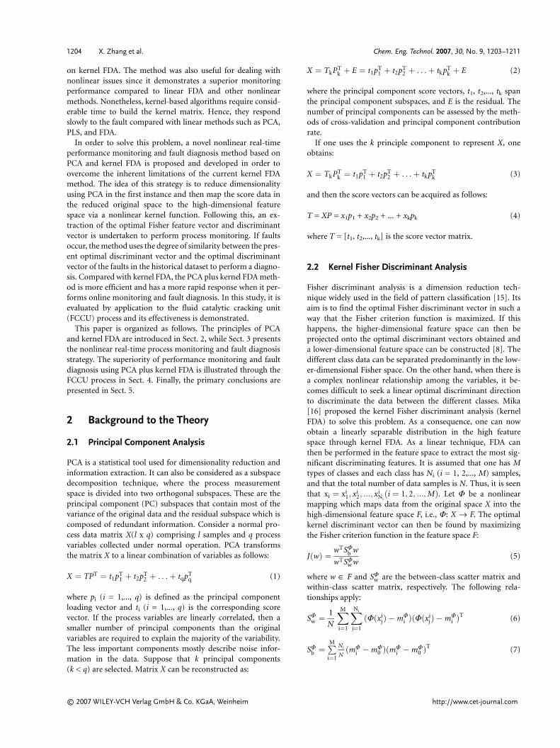
on kernel FDA. The method was also useful for dealing withnonlinear issues since it demonstrates a superior monitoringperformance compared to linear FDA and other nonlinearmethods. Nonetheless, kernel-based algorithms require consid-erable time to build the kernel matrix. Hence, they respondslowly to the fault compared with linear methods such as PCA,PLS, and FDA.

In order to solve this problem, a novel nonlinear real-timeperformance monitoring and fault diagnosis method based onPCA and kernel FDA is proposed and developed in order toovercome the inherent limitations of the current kernel FDAmethod. The idea of this strategy is to reduce dimensionalityusing PCA in the first instance and then map the score data inthe reduced original space to the high-dimensional featurespace via a nonlinear kernel function. Following this, an ex-traction of the optimal Fisher feature vector and discriminantvector is undertaken to perform process monitoring. If faultsoccur, the method uses the degree of similarity between the pres-ent optimal discriminant vector and the optimal discriminantvector of the faults in the historical dataset to perform a diagno-sis. Compared with kernel FDA, the PCA plus kernel FDA meth-od is more efficient and has a more rapid response when it per-forms online monitoring and fault diagnosis. In this study, it isevaluated by application to the fluid catalytic cracking unit(FCCU) process and its effectiveness is demonstrated.

This paper is organized as follows. The principles of PCAand kernel FDA are introduced in Sect. 2, while Sect. 3 presentsthe nonlinear real-time process monitoring and fault diagnosisstrategy. The superiority of performance monitoring and faultdiagnosis using PCA plus kernel FDA is illustrated through theFCCU process in Sect. 4. Finally, the primary conclusions arepresented in Sect. 5.

2 Background to the Theory

2.1 Principal Component Analysis

PCA is a statistical tool used for dimensionality reduction andinformation extraction. It can also be considered as a subspacedecomposition technique, where the process measurementspace is divided into two orthogonal subspaces. These are theprincipal component (PC) subspaces that contain most of thevariance of the original data and the residual subspace which iscomposed of redundant information. Consider a normal pro-cess data matrix X(l x q) comprising l samples and q processvariables collected under normal operation. PCA transformsthe matrix X to a linear combination of variables as follows:

X � TPT � t1pT1 � t2pT

2 � � � �� tqpTq (1)

where pi (i = 1,..., q) is defined as the principal componentloading vector and ti (i = 1,..., q) is the corresponding scorevector. If the process variables are linearly correlated, then asmaller number of principal components than the originalvariables are required to explain the majority of the variability.The less important components mostly describe noise infor-mation in the data. Suppose that k principal components(k < q) are selected. Matrix X can be reconstructed as:

X � TkPTk � E � t1pT

1 � t2pT2 � � � �� tkpT

k � E (2)

where the principal component score vectors, t1, t2,..., tk spanthe principal component subspaces, and E is the residual. Thenumber of principal components can be assessed by the meth-ods of cross-validation and principal component contributionrate.

If one uses the k principle component to represent X, oneobtains:

X � TkPTk � t1pT

1 � t2pT2 � � � �� tkpT

k (3)

and then the score vectors can be acquired as follows:

T = XP = x1p1 + x2p2 + ... + xkpk (4)

where T = [t1, t2,..., tk] is the score vector matrix.

2.2 Kernel Fisher Discriminant Analysis

Fisher discriminant analysis is a dimension reduction tech-nique widely used in the field of pattern classification [15]. Itsaim is to find the optimal Fisher discriminant vector in such away that the Fisher criterion function is maximized. If thishappens, the higher-dimensional feature space can then beprojected onto the optimal discriminant vectors obtained anda lower-dimensional feature space can be constructed [8]. Thedifferent class data can be separated predominantly in the low-er-dimensional Fisher space. On the other hand, when there isa complex nonlinear relationship among the variables, it be-comes difficult to seek a linear optimal discriminant directionto discriminate the data between the different classes. Mika[16] proposed the kernel Fisher discriminant analysis (kernelFDA) to solve this problem. As a consequence, one can nowobtain a linearly separable distribution in the high featurespace through kernel FDA. As a linear technique, FDA canthen be performed in the feature space to extract the most sig-nificant discriminating features. It is assumed that one has Mtypes of classes and each class has Ni (i = 1, 2,..., M) samples,and that the total number of data samples is N. Thus, it is seenthat xi � xi

1� xi2� �� xi

Ni�i � 1� 2� ��M�. Let U be a nonlinear

mapping which maps data from the original space X into thehigh-dimensional feature space F, i.e., U: X → F. The optimalkernel discriminant vector can then be found by maximizingthe Fisher criterion function in the feature space F:

J�w� � wTSUb w

wTSUw w

(5)

where w ∈ F and SUw are the between-class scatter matrix and

within-class scatter matrix, respectively. The following rela-tionships apply:

SUw � 1

N

�M

i�1

�Ni

j�1

�U�xij� � mU

i ��U�xij� � mU

i �T (6)

SUb � �M

i�1

Ni

N�mU

i � mU0 ��mU

i � mU0 �T (7)


1204 X. Zhang et al. Chem. Eng. Technol. 2007, 30, No. 9, 1203–1211

where

mUi � 1

Ni

�Ni

j�1U�xi

j� (8)

mU0 � 1

N

�Nj�1

U�xj� (9)

Since a direct computation of U(x) is not always feasible,one can introduce a kernel function:

K(xi, xj) = <U(xi), U(xj)> (10)

which permits the calculation of the value of the dot productin F without directly calculating U. The possible choices of Kinclude Gaussian and polynomial kernels. From the theory ofreproducing kernels, it is known that any solution w ∈ F mustlie in the span of all of the training samples in F. Therefore, anexpansion can be found for w of the form:

w � �Ni�1

aiU�xi� � Ua (11)

where U = (U(xi),..., U(xN)), a = (a1,... aN)T ∈ RN. By project-ing U(xi) to vector w, one obtains:

wTU(xi) = aTUTU(xi) =aT(U(x1)TU(xi),...,U(xN)TU(xi))T =aTfxi (12)

With respect to the sample vector x ∈ RN, one can define:

fx = (K(x1, x),..., K(xN, x))T (13)

which is known as the kernel sample vector. In a similarmanner, by projecting mU

i (i = 1,..., M) and mU0 to vector w,

one obtains the kernel mean vector, li (i = 1,..., M), of thewithin-class and the kernel mean vector, l0, of all mappedsamples, as follows:

li � � 1

Ni

�Ni

j�1K�x1� xi

j�� 1

Ni

�Ni

j�1K�xN� xi

j��T (14)

l0 � � 1

N

�Ni�1

K�x1� xi�� 1

N

�Ni�1

K�xN� xi��T (15)

The Fisher discriminant criteria function is equipollent to:

J�a� � aTKbaaTKwa

(16)

where

Kb � �Mi�1

Ni

N�li � l0��li � l0�T (17)

Kw � 1

N

�Mi�1

�Ni

j�1�nxi

j� li��nxi

j� li�T (18)

Kb and Kw are the kernel between-class scatter matrix andkernel within-class scatter matrix, respectively, and Eq. (16) isthe kernel Fisher discriminant criteria function. The optimalkernel Fisher discriminant , aopt, can be obtained by maximiz-ing Eq. (16). It is seen to be equipollent by solving the general-ized feature equation:

Kba = kKwa (19)

where aopt is the eigenvector corresponding to the maximaleigenvalue.

3 Process Monitoring and Fault DiagnosisBased on Principal Component Analysisand Kernel Fisher Discriminant Analysis

3.1 Principal Components

Process monitoring methods are based on PCA monitoring ofvariables in the principal and residual space by using Hotell-ing’s T2 and Q statistic. The main parameter of the T2 statisticis a kind of weighted statistical distance [17]. The monitoringmethodology based on PCA plus kernel FDA also uses distanceas a statistic. It compares the Euclidean distance of the optimalkernel Fisher feature vector between the present data and thereference data to perform performance monitoring.

Fault diagnosis was performed using contribution plots withtraditional statistical methods. However, in high-dimensionalfeature space, it is difficult or even impossible to find an in-verse mapping to the original space to calculate the contribu-tion rate of the variables. Hence, a performance monitoringmethod based on PCA plus kernel FDA performs the fault di-agnosis by using pattern matching technology instead of con-tribution plots. It is known that the optimal Fisher discrimi-nant vector extracted from a different fault is different in theFisher discriminant analysis. By calculating the degree of simi-larity between the present discriminant vector and the optimaldiscriminant vector from the historical fault dataset, one can de-cide which is most similar to the present optimal discriminantvector and it can be recognized as the present fault. In practiceapplications, a diagnosis limit of s was set. If the degree of simi-larity between the present discriminant vector and optimal vec-tor of each fault is smaller than s then it can be stated that a newfault is occurring. Therefore, one can discriminate the faultaccording to experience and add it to the historical fault dataset.

Once a developed model reflects the normal operation re-gion, it then becomes necessary to detect any departure of theprocess from its standard behavior, i.e., one must calculate theconfidence limit value to determine whether the process is incontrol or not. In PCA or PLS monitoring, Hotelling’s T2 anal-ysis and SPE charts are effective tools for extracting the criticalfeatures of the data. These analyses are based on the assump-tion that the probability density functions of the latent vari-ables follow a multivariate Gaussian distribution. However,contrary to this assumption for probability density functions,Martin and Morris [18] reported that through tests for multi-variate normality on the scores, they were able to find that thelatent variables in many industrial processes rarely have a mul-tivariate Gaussian distribution. An alternative approach to de-fine the nominal operating regions is to use data-driven tech-niques such as non-parametric empirical density estimatesusing kernel extraction [13, 18, 19]. The latent variables in thekernel FDA monitoring method do not follow a Gaussian dis-tribution either. Thus, the kernel density estimation can beused to calculate confidence limits for the D statistic.


Chem. Eng. Technol. 2007, 30, No. 9, 1203–1211 Real-time processes 1205

A univariate kernel estimator with kernel K is defined as fol-lows:

�f�x� � 1

nh

�n

i�1

Kx � xi

h

� �(20)

where x is the data point under consideration, xi is an observa-tion value from the dataset, and h is the window width. Theleast squares cross-validation (LSCV) method [13] is used toselect the value of h and n is considered as the number of ob-servations, while K is the kernel function. In practice, the formof the kernel function is not very important. In addition, theGaussian kernel function is the most commonly used type[13]. For more details concerning kernel density estimation,any interested party may refer to the works of Silverman [20]and Wand and Jones [13, 21].

The control limit used in kernel FDA monitoring charts canbe obtained using the following kernel density estimation.Firstly, the D values from normal operating data are required.Next, the univariate kernel density estimator is used to esti-mate the density function of the normal D values. The pointthat occupies 99 % of the area of the density function is ob-tained and becomes the control limit of the normal operatingdata [13, 18, 19].This point is denoted as D*.

3.2 Outline of Online Performance Monitoring andFault Diagnosis Based on PCA Plus Kernel FDA

– Step 1: Reduce the dimensionality of the original referencedataset, Xref, and new sample dataset, Xnew, using PCA. Cal-culate the score vectors using Eq. (4) and acquire the refer-ence score vector, tref, and new sample score vector, tnew.

– Step 2: Select the appropriate nonlinear kernel function andmap the reference score vector, tref, and new sample scorevector, tnew, from the original space into the high-dimen-sional feature space, and acquire the kernel reference dataset,nxref

and kernel sample dataset, nxnew.

– Step 3: Regard the kernel reference dataset, nxref, and the new

kernel sample dataset, nxnew, as different pattern classes, and

then calculate the within-class scatter matrix, Kw, and be-tween-class scatter matrix, Kb.

– Step 4: Acquire the optimal kernel Fisherdiscriminant vector, aopt, by solving thegeneralized feature equation, Eq. (19).

– Step 5: Project the kernel reference data-set, nxref

, and the kernel sample dataset,nxnew

, to the optimal kernel discriminantvector, aopt, and acquire the kernel opti-mal feature vectors, Tref and Tnew.

– Step 6: Calculate the Euclidean distancebetween the two kernel Fisher featurevectors via D � Tref � Tnew� �2.

– Step 7: If the statistic D is larger than thecontrol limit, then a fault may have oc-curred. Calculate the similar coefficient,S, to diagnose the type of faults, as fol-lows:

S � �aopt��ai�T

aopt

�� ai� � (21)

where aopt is the optimal kernel Fisher discriminant vector ofthe present dataset, and ai is the optimal kernel Fisher discri-minant vectors of the faults’ dataset (assuming that there are ntypes of faults in the faults’ dataset).

From Eq. (21), it is known that the similar coefficient, S, isthe cosine value of the two optimal kernel Fisher vectors’ an-gles.

4 Application Studies and Discussion

A fluid catalytic cracking unit or FCCU is an important eco-nomic unit in refining operations. It typically receives severaldifferent heavy feed stocks from other refinery units. More-over, it cracks these streams to produce lighter and more valu-able components that are eventually blended into gasoline andother products. The complex principles of kinetics withstrongly nonlinear and coupling among variables, ranks it asamong one of the most challenging issues in the field of pro-cess monitoring and fault diagnosis [21].

The particular Model IV unit described by McFarlane et al.is illustrated in Fig. 1. The principal feed to the unit is gas oil.However, heavier diesel and wash oil streams also contributeto the total feed stream. Fresh feed is preheated in a heat ex-changer and furnace and then passed to the riser where it ismixed with hot regenerated catalyst from the regenerator. Slur-ry from the bottom of the main fractionator is also recycled tothe riser. The gaseous cracked products are then passed to themain fractionator for separation. In the cracking process, cokeis deposited on the surface of the catalyst. Later the catalyst de-pletes its catalytic property. For this reason, spent catalyst is re-cycled to the regenerator where it is mixed with air in a fluid-ized bed for regeneration of its catalytic properties [22, 23].Complete details of the mechanistic simulation model for thisparticular model IV FCCU can be found in McFarlane et al.[24]. The process variables selected for the FCCU case studyare given in Tab. 1. A complete list of measured variables ofthe FCCU system can be found in McFarlane et al. [24].

Firstly, a group of normal data and three groups of fault data(fault 1, fault 2, and fault 3) were selected from the historical


Figure 1. Schematic diagram of the FCCU process.


dataset, which is generated from simulation studies, in theFCCU process and extracted from the first and second optimaldiscriminant vector using Fisher discriminant analysis. Thenthe data was projected to the optimal discriminant vector,which resulted in the generation of a scatter plot of the firstand second feature vector in the original space. It can be seenin Fig. 2 that only fault 1 can be differentiated clearly from thenormal data and that faults 2 and 3 cannot be differentiatedfrom normal data. The reason for this is that FDA is a linearmethod in operation. Consequently, it has a poor ability todeal with data which shows complex nonlinear relationshipamong variables. The scatter plot of the first kernel Fisher fea-ture vector and the second vector via kernel FDA is presentedin Fig. 3. It is seen from Fig. 3 that after projecting to thehigh-dimensional feature space through selecting the appro-priate kernel function, the kernel Fisher discriminant methodcan easily discriminate data that belong to different classes.

The RBF function is used as the selected kernel function, andthe parameter c is selected as 0.8 according to experience, viz:

K�xi� xj� � exp�� xi � xj

�� 2

c� (22)

The process disturbances considered are listed in Tab. 2. A10 % loss of combustion air blower capacity was selected for


Table 1. Considered process variables of the FCCU case study.

Variable Description

1 Flow of wash oil to reactor riser

2 Flow of fresh feed to reactor riser

3 Flow of slurry to reactor riser

4 Temperature of fresh feed entering furnace

5 Fresh feed temperature to riser

6 Furnace firebox temperature

7 Combustion air blower inlet suction flow

8 Combustion air blower throughput

9 Combustion air flow rate

10 Lift air blower suction flow

11 Lift air blower speed

12 Lift air blower throughput

13 Riser temperature

14 Wet gas compressor suction pressure

15 Wet gas compressor inlet suction flow

16 Wet gas flow to vapor recovery unit

17 Regenerator bed temperature

18 Stack gas valve position

19 Regenerator pressure

20 Standpipe catalyst level

21 Stack gas O2 concentration

22 Combustion air blower discharge pressure

23 Wet gas composition suction valve position

81 82 83 84 85 86 87 88 89 90117

118

119

120

121

122

123

124

First Fisher feature direction

Sec

ond

Fis

her

feat

ure

dire

ctio

n

normalfault1fault2fault3

Figure 2. Scatter plot in original feature space.

104 106 108 110 112 114 1162.4

2.6

2.8

3

3.2

3.4

3.6

3.8

4

First kernel Fisher feature direction

Sec

ond

kern

el F

ishe

r fe

atur

e di

rect

ion

normalfault1fault2fault3

Figure 3. Scatter plot in high-dimensional feature space.

Table 2. Process disturbances for FCCU.

Case Disturbance

1 10 % loss of combustion air blower capacity

2 5 % degradation in the flow of regenerated catalyst

3 5 % increase in the coke factor of the feed

4 10 % decrease in the heat exchanger coefficient of the furnace

5 10 % increase in fresh feed

6 5 % decrease in lift air blower speed

7 5 % increase in friction coefficient of regenerated catalyst

8 Negative bias of reactor pressure sensor


the simulation. The loss of combustion air blower capacity re-duces the airflow into the regenerator. Hence, this results in areduction of the regenerator pressure and further reduces theoxygen available for recycling the catalyst, which eventuallyleads to a deterioration of the reaction conditions in the riser.A data set was simulated and contained 300 data points atsampling intervals of 3 min. The disturbance was injected after150 data points of the recorded data and referred to as fault 1.

In order to demonstrate the predominance of the PCA pluskernel FDA monitoring scheme, three monitoring approacheswere investigated using the recorded dataset. Firstly, the PCAand kernel FDA were applied and this was then followed by acomparison to the PCA plus kernel FDA monitoring method.It is known that the appropriate choice of the number of prin-cipal components (PCs) is important in PCA. The number ofcomponents is determined by the cumulative percentage of thecomponents that can explain the total variance. The cumula-tive variance captured by the principal components is shownin Fig. 4. When the captured variance percentage is up to60 %, 90 %, and 99 %, the PCs are 8, 15, and 19, respectively.

When an online process monitoring is performed via kernelFDA in the FCCU process, the confidence limit value must becalculated to determine whether the process is in control ornot. Figs. 5 and 6 show the density estimate and normal prob-ability plot of the 9th latent variable vector, t9, that was calcu-lated by applying kernel FDA to the normal operation data. Itobvious that t9 does not follow a Gaussian distribution. There-fore, determining the control limit using a traditional methodwill lead to poor monitoring performance. In this paper, the99 % confidence limit D* is defined by using the kernel densityestimation strategy that has been previously proposed.

The PCA (PCs = 15) monitoring charts of T2 and SPE forfault 1 are given in Fig. 7. As the fault occurred, the monitor-ing charts showed that there is only a small response seen inthe T2 statistics. In addition, the SPE statistic can also detectthe occurrence of this fault, although it is not very obvious. Itis evident from the chart that PCA captures only the dominant


0 5 10 15 20 250.1

0.2

0.3

0.4

0.5

0.6

0.7

0.8

0.9

1

Principle components(PCs)

Var

ianc

e ca

ptur

ed

Captured 60% variance ( 8PCs)

Captured 90% variance ( 15PCs)

Captured 99% variance (19PCs)

Figure 4. Cumulative variance captured by principal componentsin PCA.

90 92 94 96 98 100 1020

0.05

0.1

0.15

0.2

0.25

0.3

0.35

0.4

0.45

0.5

The 9th latent variable

Den

sity

est

imat

e

Figure 5. Density estimate of the 9th latent variable obtainedfrom kernel FDA.

92 93 94 95 96 97 98 99 1000.003

0.01 0.02

0.05

0.10

0.25

0.50

0.75

0.90

0.95

0.98 0.99

0.997

Data

Pro

babi

lity

Normal Probability Plot

Figure 6. Normality check of the 9th latent variable obtainedfrom kernel FDA.

0 50 100 150 200 250 3000

10

20

30

40

Sample

T2

0 50 100 150 200 250 3000

20

40

60

Sample

SP

E

99% Control limit

99% Control limit

Figure 7. PCA monitoring chart for fault 1 (PCs = 15, captured90 % variance).


variation and fails to detect the small disturbance in driftsstarting from sample 150.

Fig. 8 shows the monitoring chart obtained using kernelFDA for fault 1. It is clear from Fig. 8 that the kernel FDA hasa relatively distinct response to the occurrence of fault 1 at ca.sample 150. This is almost the same time that the fault oc-curred. Since the kernel FDA is a nonlinear method, it pos-sesses a better ability to deal with nonlinear data. This is thereason behind its better monitoring performance.

The monitoring results of fault 1 using PCA plus kernelFDA with PCs equal to 8, 19, and 15 in PCA are shown inFigs. 9–11, respectively. From Figs. 9–11, it is seen that PCA +KFDA with PCs equal to 15 have the best detection results,Fig. 11. It captures the main information of the process (90 %variance) and discards the random noise (the remaining 10 %variance). The statistic distance increased drastically when thefault occurred at sample 150 and exceeded the 99 % controllimit. Compared with either the PCA or kernel FDA method,the PCA plus KFDA method is more effective. Moreover, itdemonstrates a quicker and clearer response to the faults.However, when the PCs are equal to 8, the detection result isnot superior to the traditional KFDA method. The reason forthis is that when the PCs are equal to 8 in PCA, the methodonly captures 60 % of the total variance, i.e., some of the usefulinformation is lost. Therefore, if online monitoring is to beperformed, the appropriate choice of PC numbers is fairly im-portant. When the PCs are equal to 19, the method captures99 % of the total variance. This is almost equivalent to notdealing with PCA. As a consequence, the monitoring result issimilar to the traditional KFDA method.

After the fault occurred, it uses the degree of similarity be-tween the present optimal discriminant vector and the optimalvector for faults in the historical dataset to perform fault diag-nosis. Fig. 12 shows that the present optimal kernel Fisher vec-tor is more similar to fault 1 than others and this similar valueis 0.93. Subsequently, it was determined that the fault resultedfrom the loss of the combustion air blower capacity (fault 1).

All eight types of faults listed in Tab. 2 were selected to per-form monitoring and fault diagnosis for comparison. Its pur-


0 50 100 150 200 250 3000

0.005

0.01

0.015

0.02

0.025

0.03

0.035

0.04

Sample

Dis

tanc

e

99% Control limit

Figure 8. Kernel FDA monitoring chart for fault 1.

0 50 100 150 200 250 3000

0.002

0.004

0.006

0.008

0.01

0.012

0.014

0.016

0.018

Sample

Dis

tanc

e

99% Control limit

Figure 9. PCA plus KFDA monitoring for fault 1 (PCA PCs = 8,captured 60 % variance).

0 50 100 150 200 250 3000

0.005

0.01

0.015

0.02

0.025

Sample

Dis

tanc

e

99% Control limit

Figure 10. PCA plus KFDA monitoring for fault 1 (PCA PCs = 19,captured 99 % variance).

0 50 100 150 200 250 3000

0.01

0.02

0.03

0.04

0.05

0.06

Sample

Dis

tanc

e

99% Control limit

Figure 11. PCA plus KFDA Monitoring for fault 1 (PCA PCs = 15,captured 90 % variance).


pose is to verify the efficiency of the PCA plus kernel FDAmethod. The results that indicate the time consumed areshown in Tab. 3. From Tab. 3, it is seen that the proposedmethod is competitive with kernel FDA. The computationtime is different with the different numbers of PCs reserved inPCA. The time consumed becomes longer with the increase ofPCs. Although the entire time consumed owith PCA plusKFDA is longer than PCA, it is much less than that for the ker-nel FDA method alone. The results show that if one choosesthe appropriate number of PCs, then the proposed method ismore preferable for real-time process monitoring and fault di-agnosis.

In order to evaluate the ability of the proposed approach toidentify disturbance, the detection results were classified as 4levels (A, B, C, and D) and listed as follows:– A: The method can detect the occurrence of the disturbance

and the result is excellent.– B: The method can detect the occurrence of the disturbance

and the result is clear.– C: The method can detect the occurrence of the disturbance

and the result is not very clear.


1 2 3 4 5 6 7 80

0.1

0.2

0.3

0.4

0.5

0.6

0.7

0.8

0.9

1

Case 1

Sim

ilar

degr

ee

Figure 12. Degree of similarity of case 1 in the historical dataset.

Table 3. Comparison of the time consumed for fault detection and diagnosis between PCA, KFDA and PCA + KFDA.

Fault Number Time consumed (s)

PCs = 8 (60 % variance) PCs = 15 (95 % variance) PCs = 19 (99 % variance)

PCA PCA + KFDA PCA PCA + KFDA PCA PCA + KFDA KFDA

1 5.2 14.1 5.4 23.7 5.5 36.2 56.3

2 4.7 13.9 4.8 21.2 4.8 32.1 51.7

3 5.0 13.4 5.1 22.1 5.0 34.4 53.6

4 6.0 16.8 6.3 27.1 6.1 45.2 64.3

5 5.5 14.7 5.7 24.6 5.5 36.8 59.5

6 5.1 14.1 5.2 23.9 5.1 35.1 57.4

7 5.1 14.9 5.3 24.2 5.2 35.8 58.9

8 5.8 16.2 6.1 26.5 6.0 43.9 61.5

Table 4. Comparison of fault detection ability among PCA, KFDA and PCA + KFDA.

Fault Number Detection Results

PCs = 8 (60 % variance) PCs = 15 (95 % variance) PCs = 19 (99 % variance)

PCA PCA + KFDA PCA PCA + KFDA PCA PCA + KFDA KFDA

1 C B C A C B B

2 D B C A D A A

3 D B C A C B B

4 C A B A C A A

5 C A B A C A A

6 B B C B B B B

7 C B C A C B B

8 D B B A C A A


– D: The method cannot detect the occurrence of the distur-bance.The detection results of PCA, KFDA, and PCA + KFDA at

different conditions are shown in Tab. 4. From Tab. 4, it isclear that the PCA + KFDA method with PCs = 15 has the bestdetection results. The same method with PCs = 8 is not asgood as the traditional KFDA approach. The reason for this isthat when the PCs are equal to 15 in PCA, it captures the maininformation of the process (90 % variance) and discards therandom noise (the remaining 10 % variance). However, whenthe PCs are equal to 8, the method only captures 60 % of thetotal variance, thereby resulting in the loss of useful informa-tion. Subsequently, if online monitoring is performed, the ap-propriate choice of PC numbers is important. The conclusionsare similar to previous analysis by the current authors andfurther verify the validity of the proposed method.

5 Conclusions

In this paper, a new real-time process monitoring and fault di-agnosis method based on PCA plus kernel FDA was developed.The basic idea of this method is to first reduce dimensionalityusing PCA, and then map the score data in the reduced origi-nal space to the high-dimensional feature space via a nonlinearkernel function, and finally to extract the optimal Fisher fea-ture vector and discriminant vector to perform process moni-toring. If faults occurred, it uses the degree of similarity be-tween the present discriminant vector and the optimaldiscriminant vector of faults in the historical dataset to per-form a diagnosis. Moreover, the time consumed by the PCAplus kernel FDA method is much less than that for the kernelFDA method alone when online monitoring is performed. Fi-nally, the simulation results of the FCCU process prove thatthe proposed method is very effective.

Acknowledgements

The authors gratefully acknowledge the support of the NaturalScience Foundation of China (60504033). The constructive ad-vice of the anonymous referees is also gratefully acknowledged.

References

[1] P. Nomikos, J. F. MacGregor, AIChE J. 1994, 40 (8), 1361.[2] W. Ku, R. H. Storer, C. Georgakis, Chemom. Intell. Lab. Syst.

1995, 30, 179.[3] B. M. Wise, N. B. Gallagher, J. Process Control 1996, 6 (6),

329.[4] D. Dong, T. J. McAvoy, Comput. Chem. Eng. 1996, 20 (1), 65.[5] B. R. Bakshi, AIChE J. 1998, 44 (7), 1596.[6] L. H. Chiang, E. L. Russell, R. D. Braatz, Chemom. Intell.

Lab. Syst. 2000, 50, 243.[7] L. H. Chiang, E. L. Russell, R. D. Braatz, Fault Detection and

Diagnosis in Industrial Systems, Springer-Verlag, New York2001.

[8] Q. P. He, S. J. Qin, J. Wang, AIChE J. 2005, 51 (2), 555.[9] M. A. Kramer, AIChE J. 1991, 37 (2), 233.

[10] D. Dong, T. J. McAvoy, Comput. Chem. Eng. 1996, 20 (1), 65.[11] F. Jia, E. B. Martin, A. J. Morris, Int. J. Syst. Sci. 2001, 31,

1473.[12] H. G. Hiden, M. J. Willis, M. T. Tham, G. A. Montague,

Comput. Chem. Eng. 1999, 23, 413.[13] J. M. Lee et al., Chem. Eng. Sci. 2004, 59, 223.[14] X. Zhang, W. Yan, X. Zhao, H. Shao, unpublished.[15] R. O. Duda, P. E. Hart, D. G. Stork, Pattern Classification.

2nd ed., John Wiley & Sons, New York 2001.[16] S. Mika et al., IEEE Int. Workshop on Neural Networks for Sig-

nal Processing, Madison, WI, August 1999.[17] R. A. Johnson, D. W. Wichern, Applied Multivariate Statisti-

cal Analysis, 3rd ed., Prentice-Hall Englewood Cliffs, NJ1992.

[18] E. B. Martin, A. J. Morris, J. Process Control 1996, 6 (6), 349.[19] Q. Chen, R. J. Wynne, P. Goulding, D. Sandoz, Control Eng.

Practice 2000, 8, 531.[20] B. W. Silverman, Density Estimation for Statistics and Data

Analysis, Chapman and Hall, London 1986.[21] M. P. Wand, M. C. Jones, Kernel Smoothing; Chapman and

Hall, London 1995.[22] X. Wang, U. Kruger, B. Lennox, Control Eng. Practice 2003,

11, 613.[23] X. Wang, U. Kruger, W. I. George, Ind. Eng. Chem. Res. 2005,

44, 5691.[24] R. C. McFarlane, R. C. Reineman, J. F. Bartee, C. Georgakis,

Comput. Chem. Eng. 1993, 17 (3), 275.



nonlinear real-time process monitoring and fault diagnosis based on principal component analysis and...

Documents