Discriminant Analysis

Chapter 18

Content

• Fisher discriminant analysis

• Maximum likelihood method

• Bayes formula discriminant analysis

• Bayes discriminant analysis

• Stepwise discriminant analysis

 

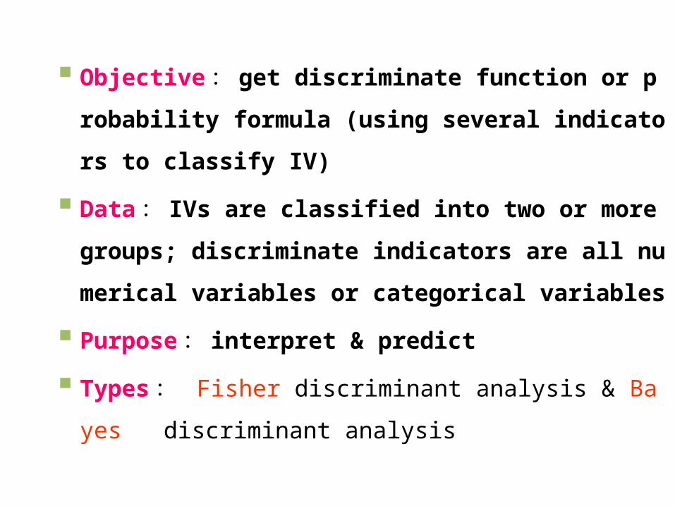
Objective ： get discriminate function or probabilit

y formula (using several indicators to classify IV)

Data ： IVs are classified into two or more groups;

discriminate indicators are all numerical variables o

r categorical variables

Purpose ： interpret & predict

Types ： Fisher discriminant analysis & Bayes discr

iminant analysis

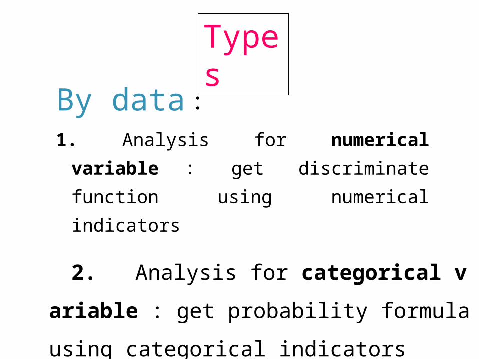
By data ：

1. Analysis for numerical variable ： get

discriminate function using numerical

indicators

Types

2. Analysis for categorical variable : get prob

ability formula using categorical indicators

By name

• Fisher discriminant analysis

• Maximum likelihood method

• Bayes formula discriminant analysis

• Bayes discriminant analysis

• Stepwise discriminant analysis

§1    Fisher Discriminant Analysis

Indicator: numerical indicator Discriminated into: two or more categories

I

discriminate into two categories

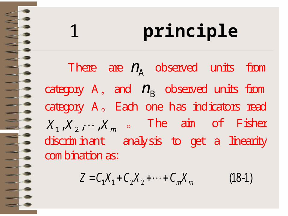
1 principle

There are An observed units from

category A，and Bn observed units from

category A。 Each one has indicators read

mXXX ,,, 21 。 The aim of Fisher

discriminant analysis to get a linearity combination as：

1 1 2 2 (18-1)m mZ C X C X C X

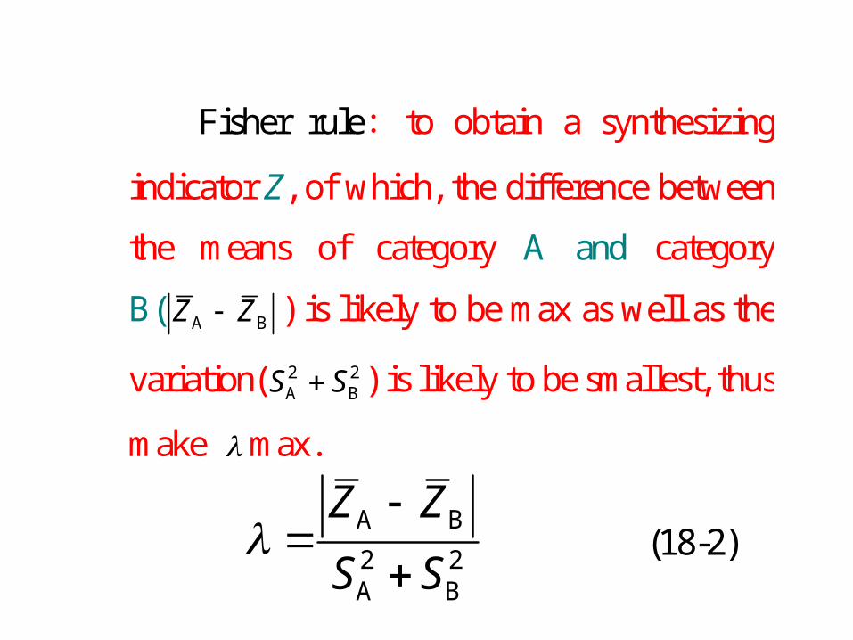
Fisher rule： to obtain a synthesizing

indicator Z, of which, the difference between

the means of category A and category

B( A BZ Z ) is likely to be max as well as the

variation( 2 2A BS S ) is likely to be smallest, thus

make max.

A B

2 2A B

Z Z

S S

(18-2)

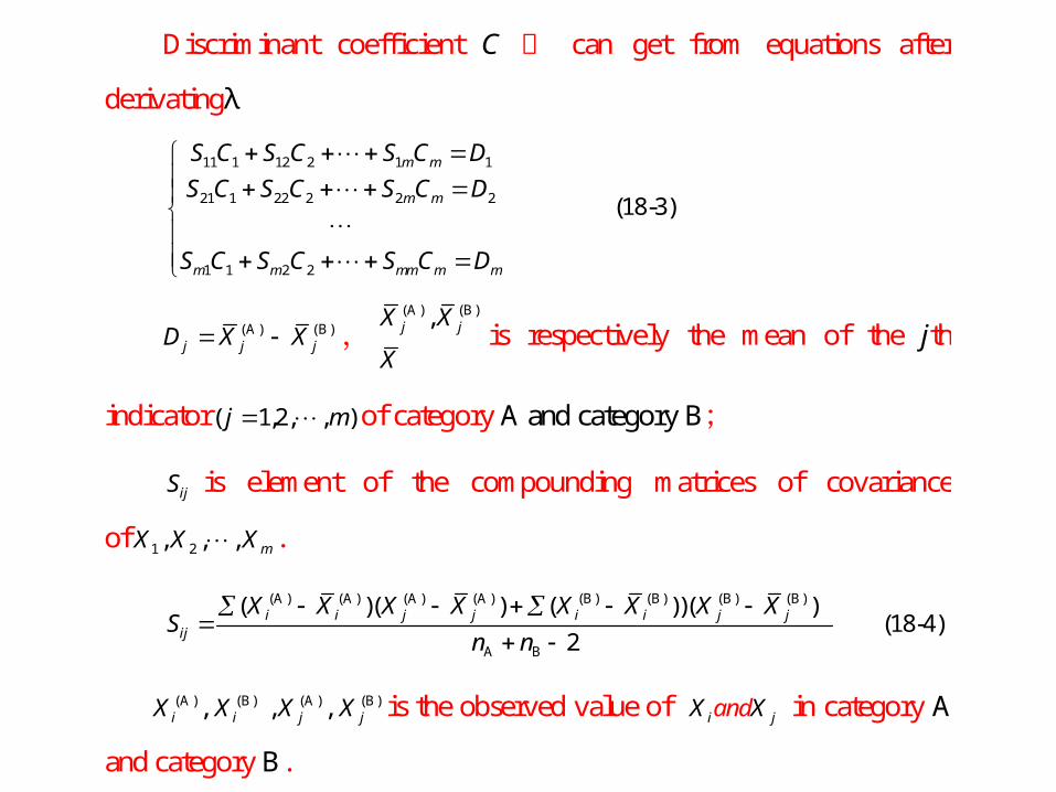
Discriminant coefficient C 可 can get from equations after

derivatingλ

11 1 12 2 1 1

21 1 22 2 2 2

1 1 2 2

(18-3)

m m

m m

m m mm m m

S C S C S C D

S C S C S C D

S C S C S C D

(A) (B)j j jD X X ，

(A) (B),j jX X

Xis respectively the mean of the jth

indicator ),,2,1( mj of category A and category B；

ijS is element of the compounding matrices of covariance

of 1 2, , , mX X X .

(A) (A) (A) (A) (B) (B) (B) (B)

A B

( )( ) ( ))( ) (18-4)

2i i j j i i j j

ij

X X X X X X X XS

n n

(A) (B) (A) (B), , , i i j jX X X X is the observed value of i jX andX in category A

and category B.

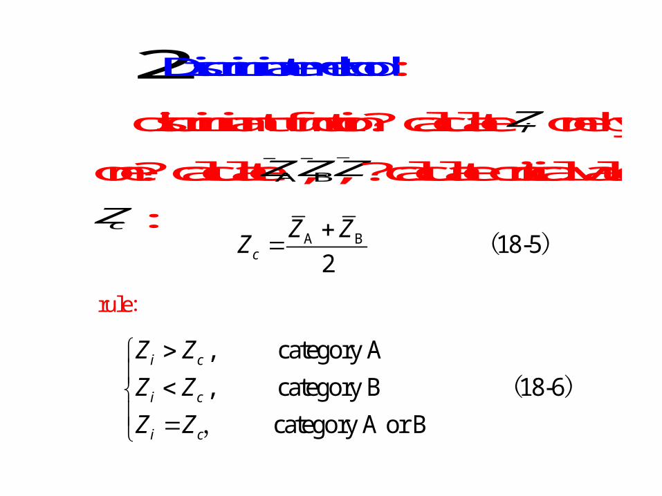
2 Discriminate method :

discriminant function? calculate iZ one by

one? calculateAZ,BZ,Z?calculate critical value

cZ : A B 18-5

2

c

Z ZZ （ ）

rule：

, category A

, category B 18-6

category A or B

i c

i c

i c

Z Z

Z Z

Z Z

（ ），

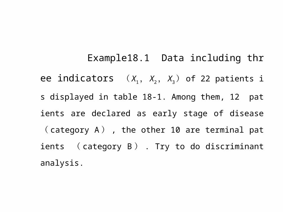
Example18.1 Data including three indicators

（ X1 ， X2 ， X3 ） of 22 patients is displayed in table 18-

1. Among them, 12 patients are declared as early stage of

disease （ category A ） , the other 10 are terminal patie

nts （ category B ） . Try to do discriminant analysis.

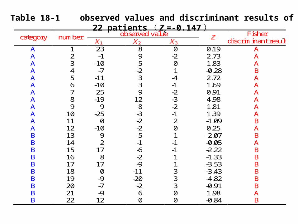
observed value category number X1 X2 X3

Z Fisher discriminant result

A 1 23 8 0 0.19 A A 2 -1 9 -2 2.73 A A 3 -10 5 0 1.83 A A 4 -7 -2 1 -0.28 B A 5 -11 3 -4 2.72 A A 6 -10 3 -1 1.69 A A 7 25 9 -2 0.91 A A 8 -19 12 -3 4.98 A A 9 9 8 -2 1.81 A A 10 -25 -3 -1 1.39 A A 11 0 -2 2 -1.09 B A 12 -10 -2 0 0.25 A B 13 9 -5 1 -2.07 B B 14 2 -1 -1 -0.05 A B 15 17 -6 -1 -2.22 B B 16 8 -2 1 -1.33 B B 17 17 -9 1 -3.53 B B 18 0 -11 3 -3.43 B B 19 -9 -20 3 -4.82 B B 20 -7 -2 3 -0.91 B B 21 -9 6 0 1.98 A B 22 12 0 0 -0.84 B

Table 18-1 observed values and discriminant results of 22 patients （ Zc=-0.147 ）

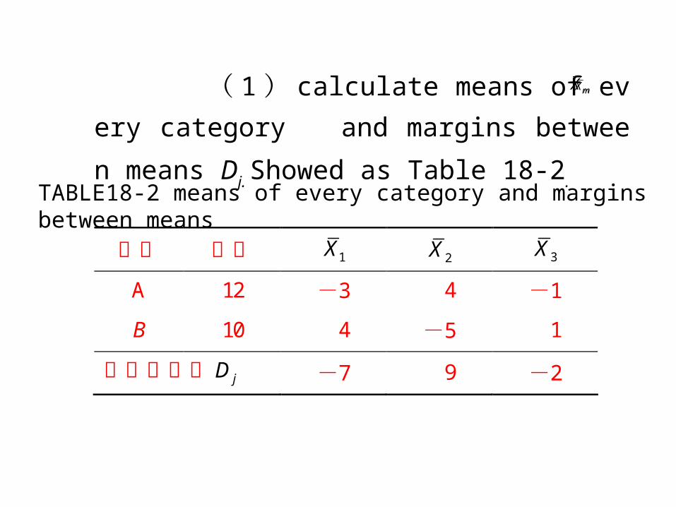
类别 例数 1X 2X 3X

A 12 －3 4 －1

B 10 4 －5 1

类间均值差 jD －7 9 －2

TABLE18-2 means of every category and margins between means

（ 1 ） calculate means of every category and

margins between means Dj. Showed as Table 18-2.

mX mX

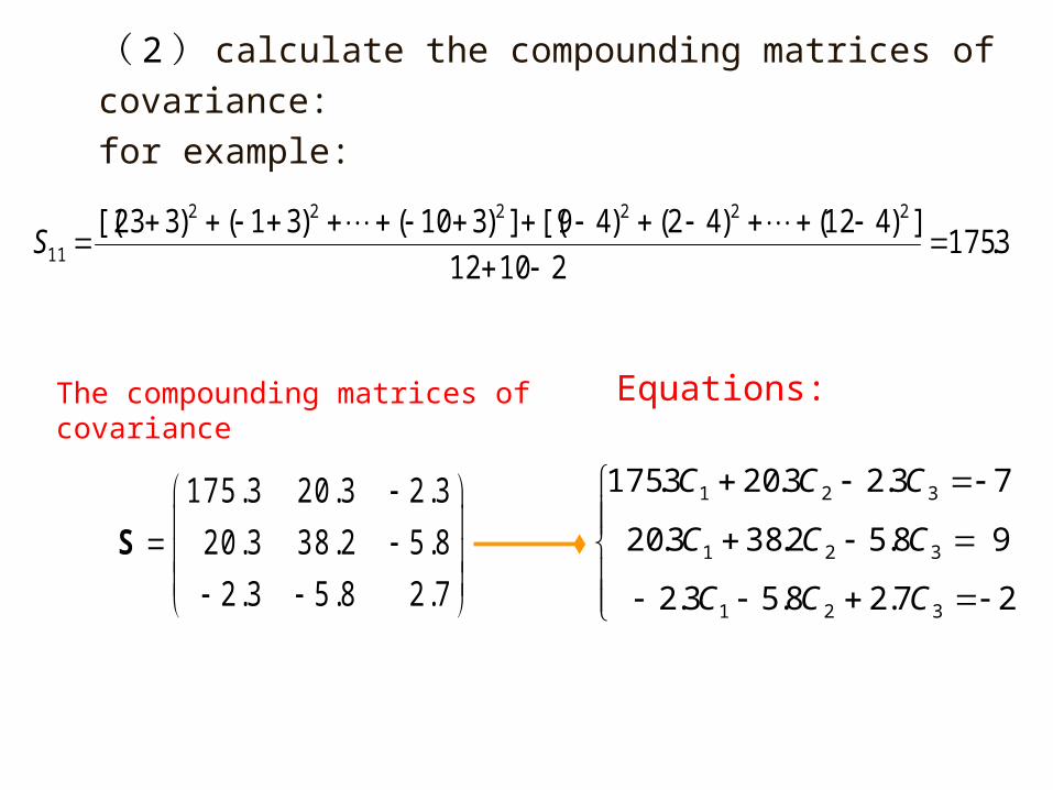
（ 2 ） calculate the compounding matrices of covariance:

for example:

3.17521012

])412()42()49[(])310()31()323[( 222222

11

S

1 7 5 .3 2 0 .3 2 .3

2 0 .3 3 8 .2 5 .8

2 .3 5 .8 2 .7

S

Equations:

27.28.53.2

9 8.52.383.20

73.23.203.175

321

321

321

CCC

CCC

CCC

The compounding matrices of covariance

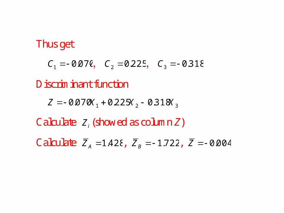
Thus get

070.01 C ， 225.02 C ， 318.03 C

Discriminant function

321 318.0225.0070.0 XXXZ

Calculate iZ (showed as column Z)

Calculate 428.1AZ , 722.1BZ , 004.0Z

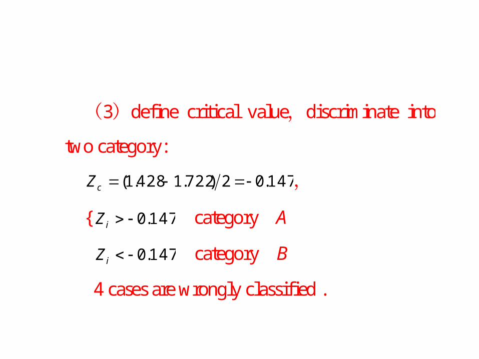
（3）define critical value，discriminate into

two category:

147.02)722.1428.1( cZ ，

{ 147.0iZ category A

147.0iZ category B

4 cases are wrongly classified .

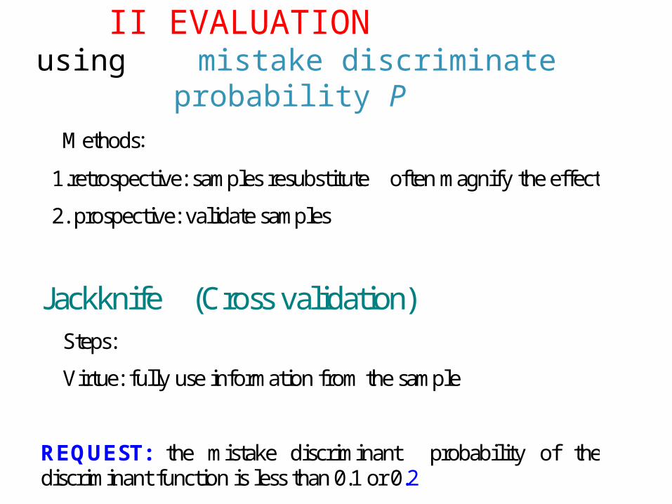
II EVALUATION using mistake discriminate probability P

Methods：

1.retrospective: samples resubstitute often magnify the effect

2. prospective: validate samples

Jackknife (Cross validation) Steps:

Virtue: fully use information from the sample

REQUEST: the mistake discriminant probability of the discriminant function is less than 0.1 or 0.2

§2    MAXIMUM LIKELIHOOD METHOD

Indicator: qualitative indicator Discriminated into: two or more

categories

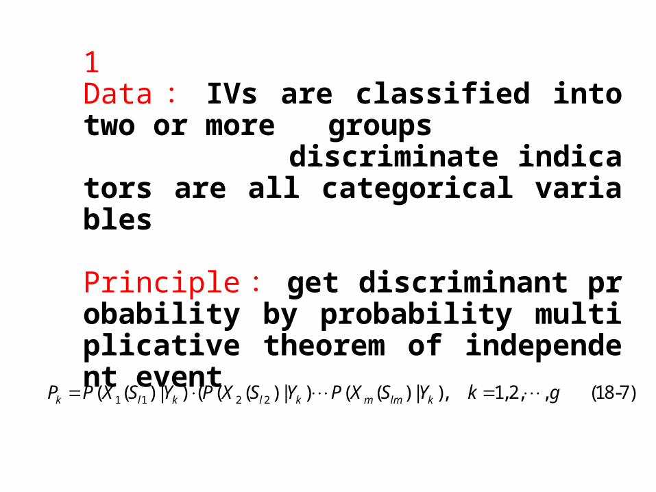
1Data ： IVs are classified into two or more groups discriminate indicators are all categorical variables

Principle ： get discriminant probability by probability multiplicative theorem of independent event

1 1 2 2( ( ) | ) ( ( ( ) | ) ( ( ) | ), 1, 2, , (18-7)k l k l k m lm kP P X S Y P X S Y P X S Y k g

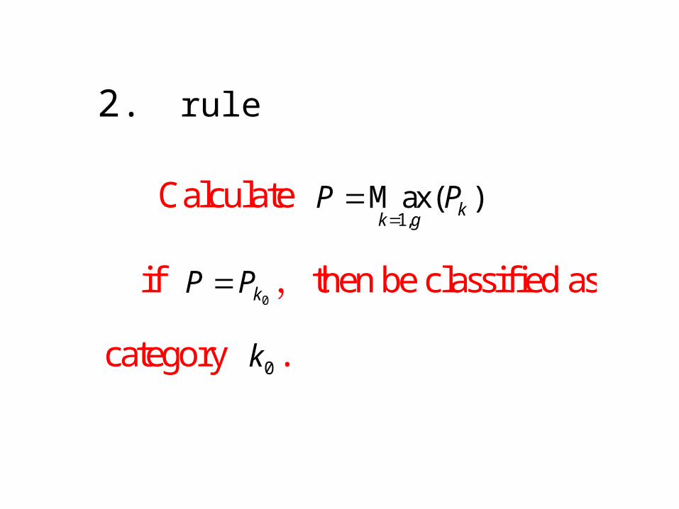
Calculate 1,

M ax( )kk g

P P

if 0kPP ，then be classified as

category 0k .

2. rule

3 application

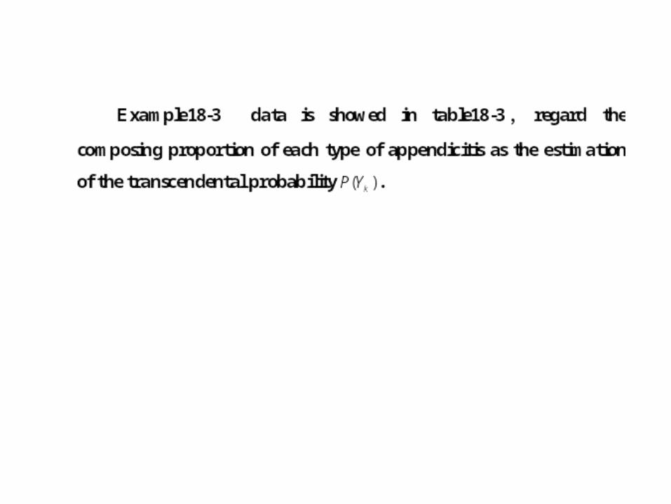
Example18.2 Someone want to use 7 indicators to

diagnose 4 types of appendicitis. 5668 medical

records are summed up in table 18-3.

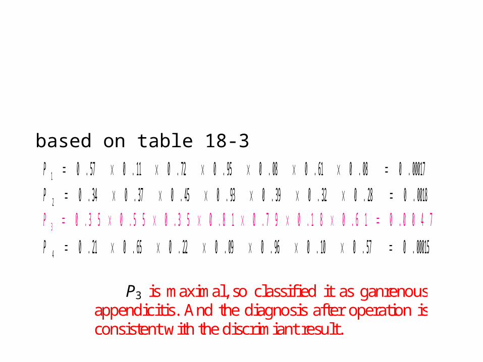
00017.008.061.008.095.072.011.057.01 P 0018.028.032.039.093.045.037.034.02 P

3 0 . 3 5 0 . 5 5 0 . 3 5 0 . 8 1 0 . 7 9 0 . 1 8 0 . 6 1 0 . 0 0 4 7P 00015.057.010.096.009.022.065.021.04 P

P3 is maximal, so classified it as ganrenous appendicitis. And the diagnosis after operation is consistent with the discrimiant result.

based on table 18-3

§ 3 Bayes formula discriminance

Indicator: qualitative indicator

Discriminated into: two or more

categories

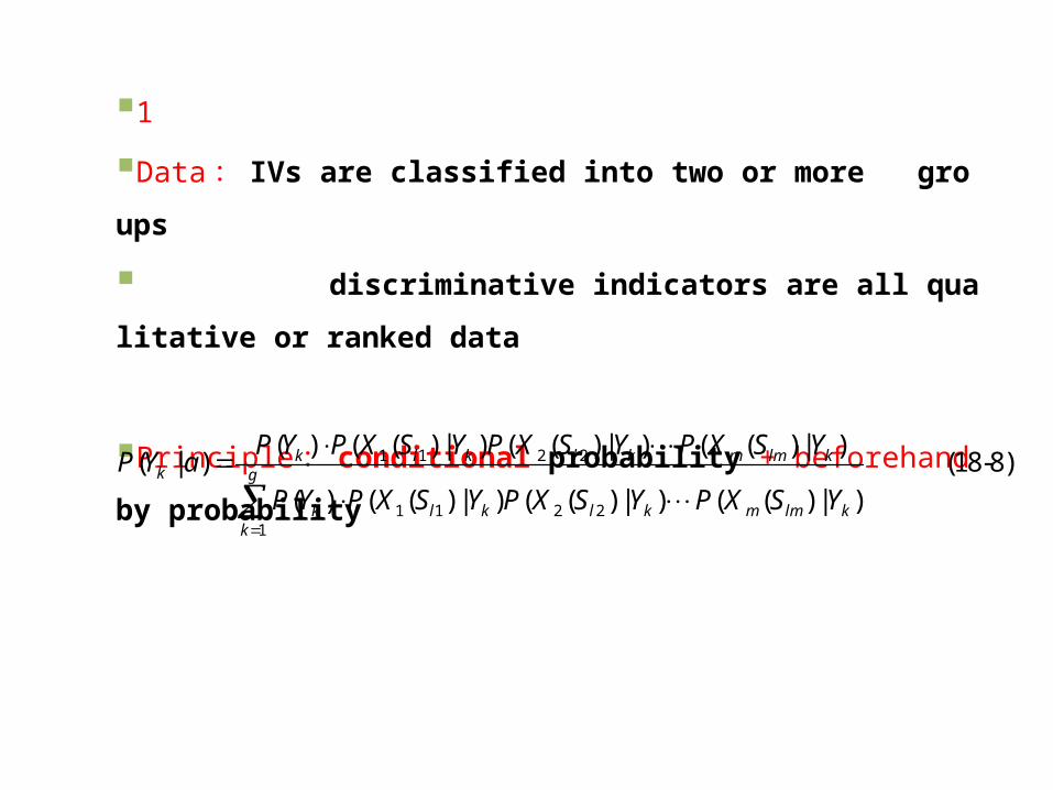
1

Data ： IVs are classified into two or more groups

discriminative indicators are all qualitative or ranked data

Principle ： conditional probability + beforehand by probability

1 1 2 2

1 1 2 21

( ) ( ( ) | ) ( ( ) | ) ( ( ) | )( | ) (18-8)

( ) ( ( ) | ) ( ( ) | ) ( ( ) | )

k l k l k m lm kk g

k l k l k m lm kk

P Y P X S Y P X S Y P X S YP Y a

P Y P X S Y P X S Y P X S Y

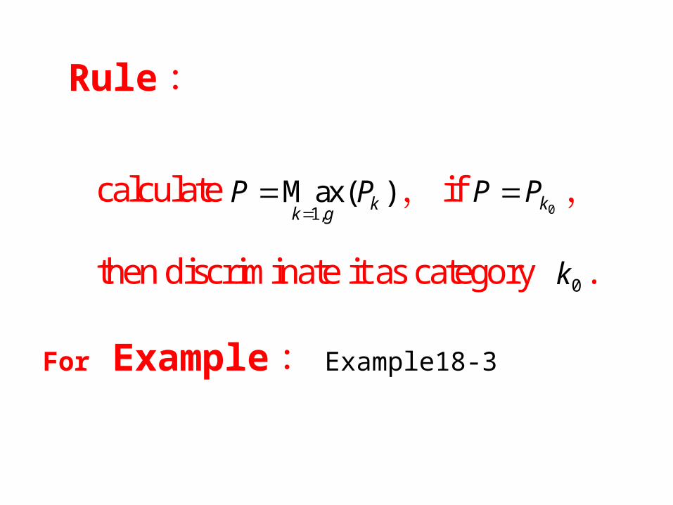
calculate1,

M ax( )kk g

P P

， if0kPP ，

then discriminate it as category 0k .

Rule ：

For Example ： Example18-3

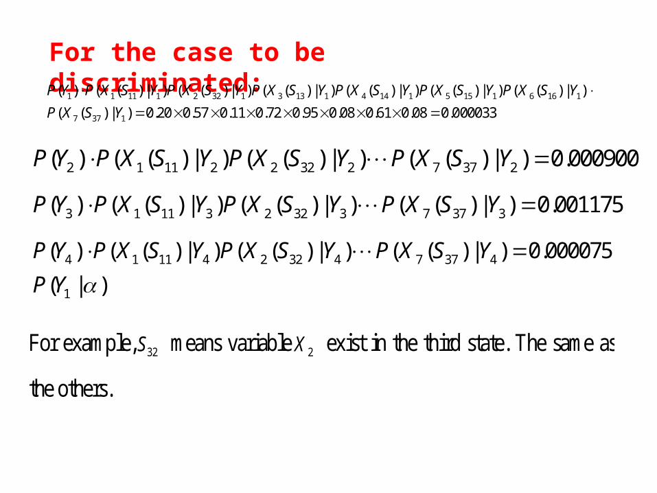
For the case to be discriminated:

1 1 11 1 2 32 1 3 13 1 4 14 1 5 15 1 6 16 1

7 37 1

( ) ( ( ) | ) ( ( ) | ) ( ( ) | ) ( ( ) | ) ( ( ) | ) ( ( ) | )

( ( ) | ) 0.20 0.57 0.11 0.72 0.95 0.08 0.61 0.08 0.000033

P Y P X S Y P X S Y P X S Y P X S Y P X S Y P X S Y

P X S Y

2 1 11 2 2 32 2 7 37 2( ) ( ( ) | ) ( ( ) | ) ( ( ) | ) 0.000900P Y P X S Y P X S Y P X S Y

3 1 11 3 2 32 3 7 37 3( ) ( ( ) | ) ( ( ) | ) ( ( ) | ) 0.001175P Y P X S Y P X S Y P X S Y

4 1 11 4 2 32 4 7 37 4

1

( ) ( ( ) | ) ( ( ) | ) ( ( ) | ) 0.000075

( | )

P Y P X S Y P X S Y P X S Y

P Y

For example, 32S means variable 2X exist in the third state. The same as

the others.

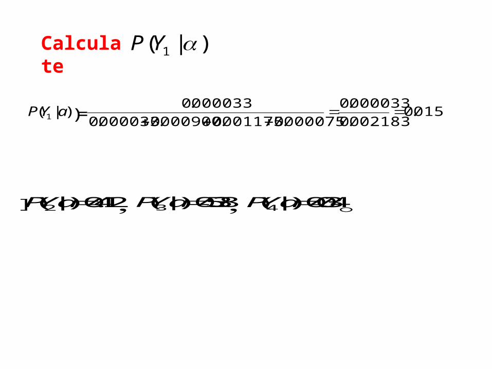
Calculate

1( | )PY a )= 015.0002183.0

000033.0

000075.0001175.0000900.0000033.0

000033.0

同样的2( | ) 0.412PYa ，3( | ) 0.538PYa ，4( | ) 0.034PYa 。

1( | )P Y

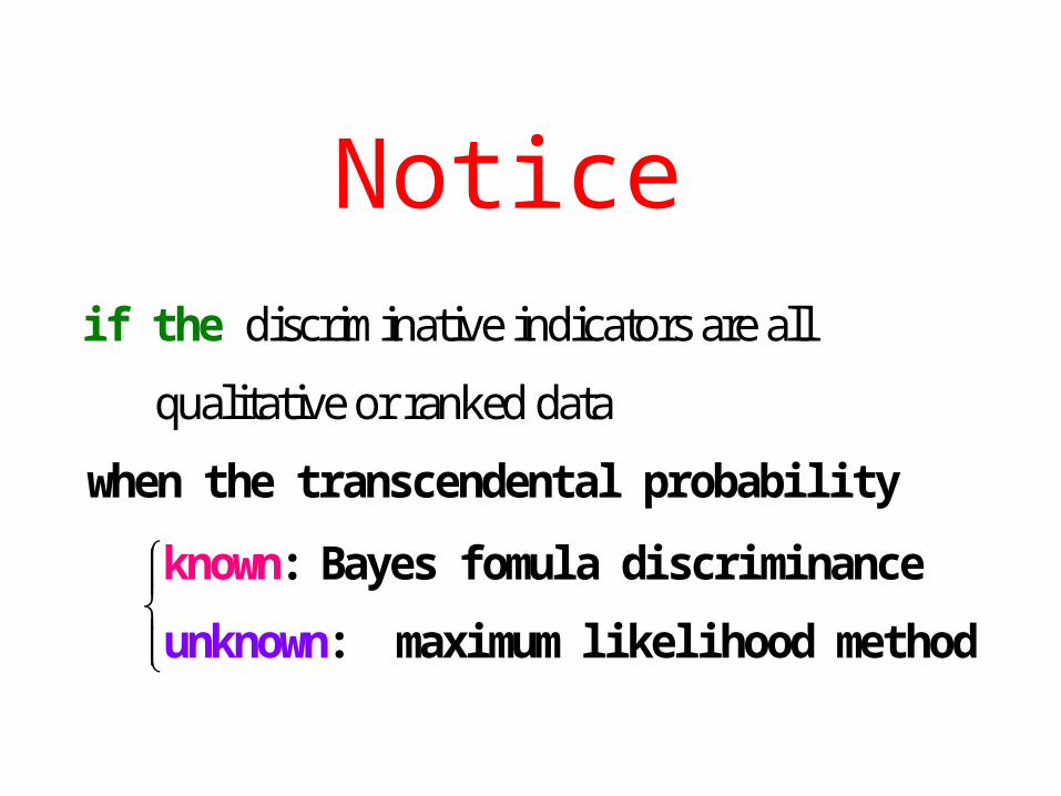
discriminative indicators are all

qualitative or ranked data

when the transcendental probabi l i ty

: Bayes fomula di scriminance

: maximum l i kelunkno ihood

i f the

metho

kn

dwn

own

Notice

§ 4 Bayes discriminant analysis

Indicator: numerical indicator

Discriminated into: several categories

(also two categories)

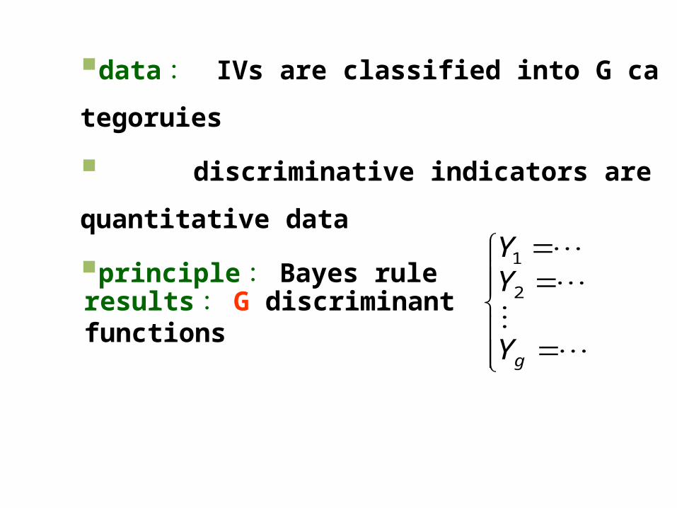
data ： IVs are classified into G categoruies

discriminative indicators are quantitative data

principle ： Bayes rule

results ： G discriminant functions

1

2

g

YY

Y

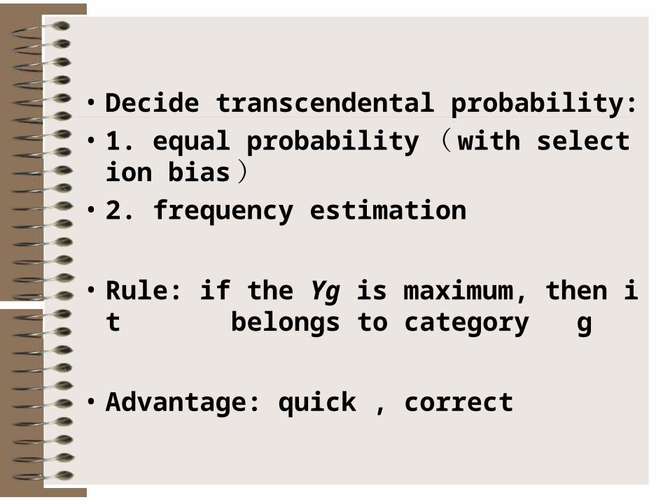
• Decide transcendental probability:• 1. equal probability （ with selection bias ）• 2. frequency estimation

• Rule: if the Yg is maximum, then it belongs to category g

• Advantage: quick , correct

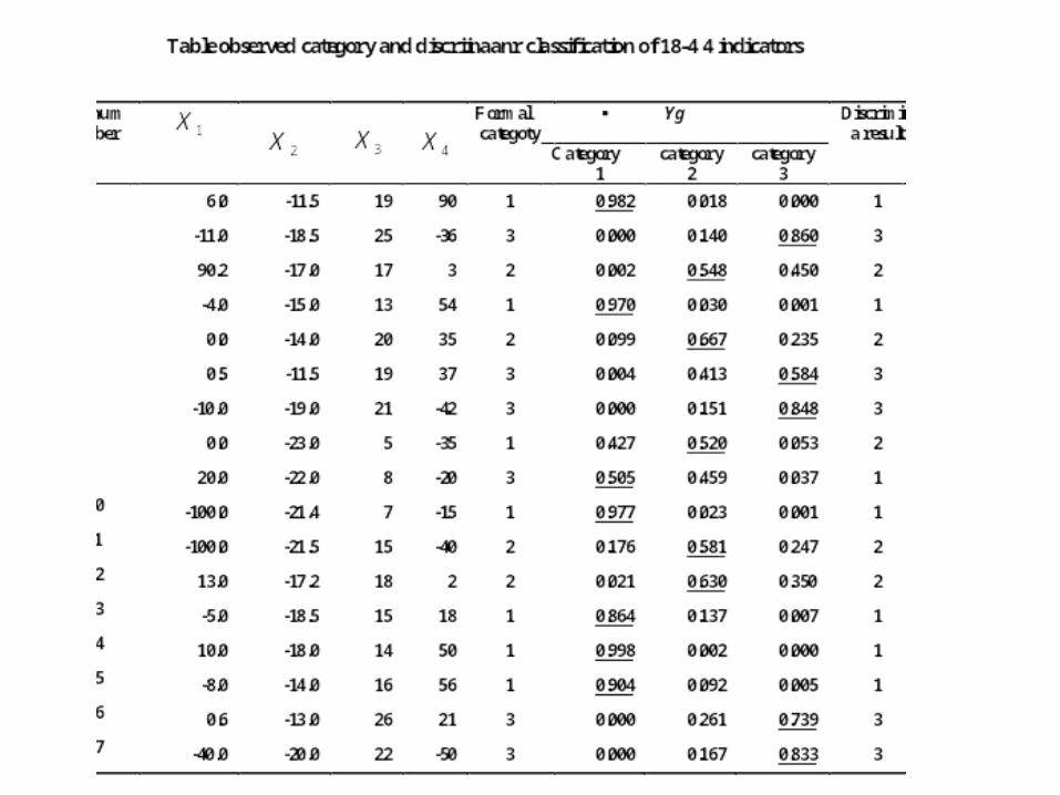
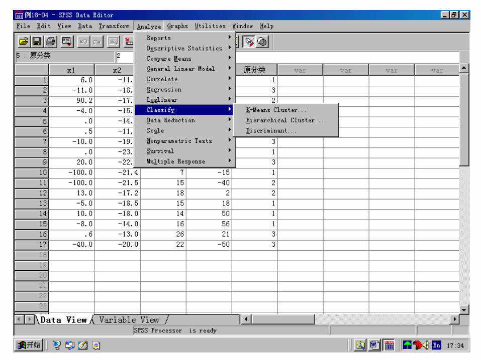
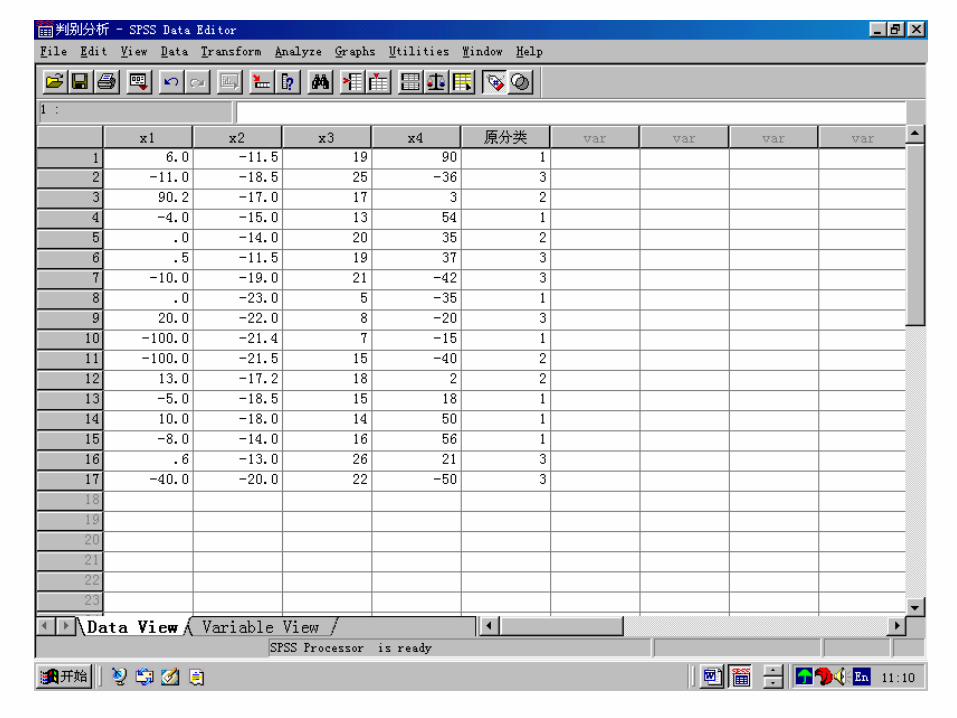
•Example18-4 Use 17 medical records sorted as table18-4 to discriminate 3 diseases. Four indicators have been list out. You are suggested to set Bayes discriminant function.

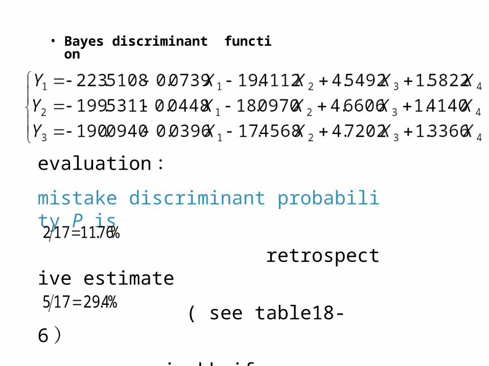
• Bayes discriminant function

evaluation ：

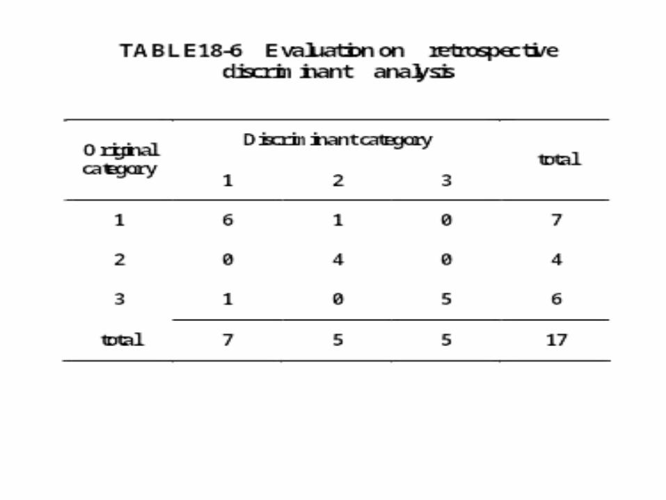
mistake discriminant probability P is

retrospective estimate

( see table18-6 ）

jackknife

%76.11172

%4.29175

§ 5 stepwise discriminant analysis

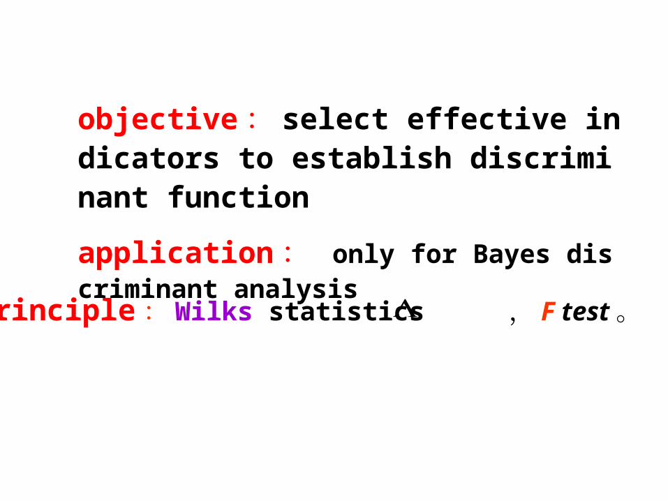
objective ： select effective indicators to establish discriminant function

application ： only for Bayes discriminant analysis

principle ： Wilks statistics ， F test 。

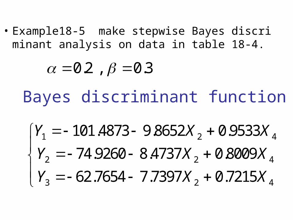
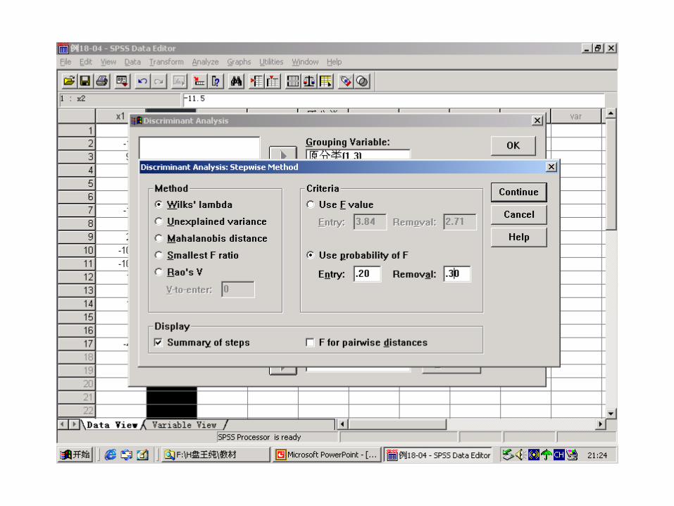
• Example18-5 make stepwise Bayes discriminant analysis on data in table 18-4.

0.2 , 0.3

Bayes discriminant function ：

1 2 4

2 2 4

3 2 4

101.4873 9.8652 0.9533

74.9260 8.4737 0.8009

62.7654 7.7397 0.7215

Y X X

Y X X

Y X X

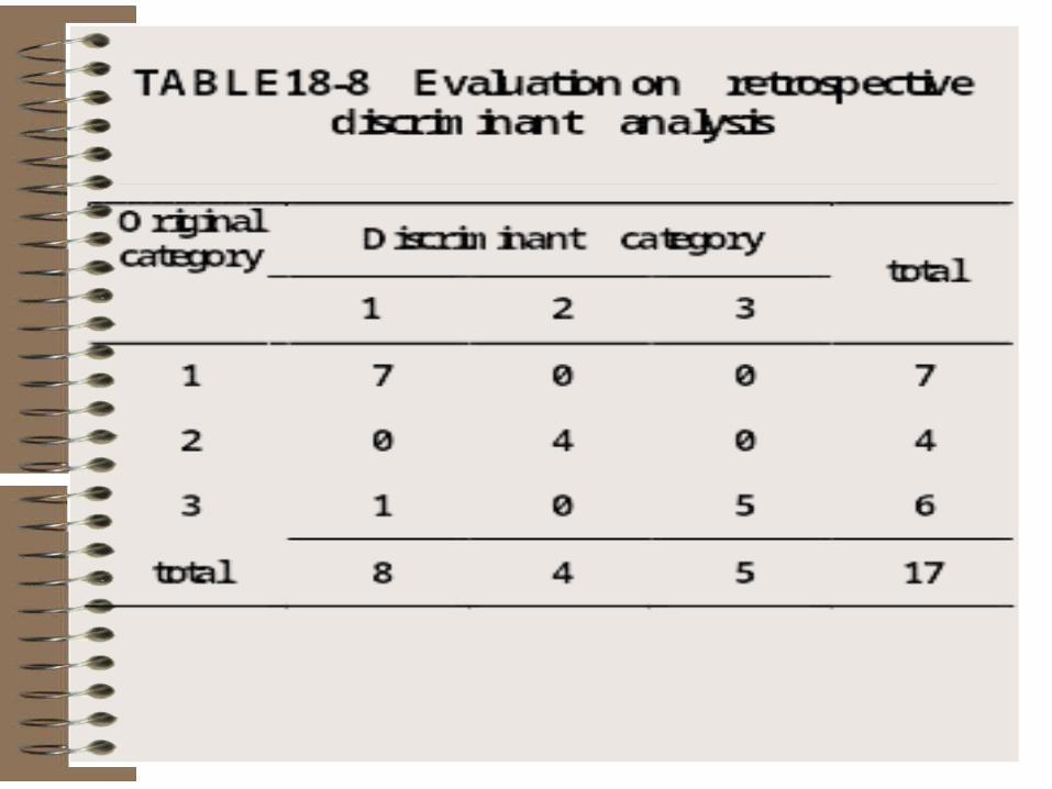
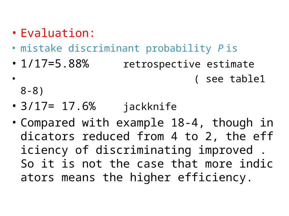
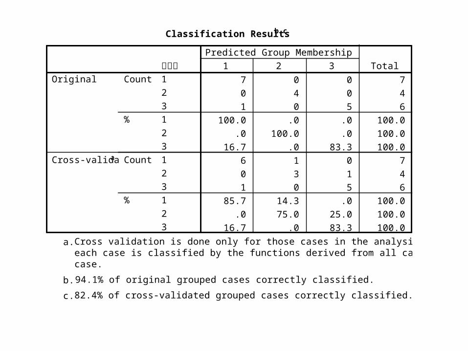
• Evaluation:• mistake discriminant probability P is

• 1/17=5.88% retrospective estimate

• ( see table18-8)

• 3/17= 17.6% jackknife

• Compared with example 18-4, though indicators reduced from 4 to 2, the efficiency of discriminating improved . So it is not the case that more indicators means the higher efficiency.

§ 6 NOTICES

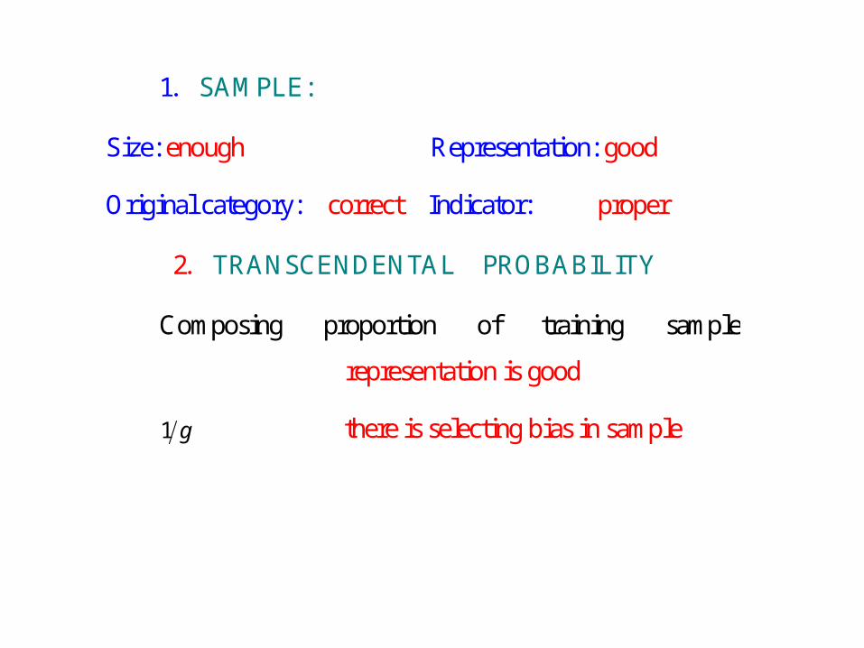
1．SAMPLE:

Size: enough Representation: good

Original category: correct Indicator: proper

2．TRANSCENDENTAL PROBABILITY

Composing proportion of training sample

representation is good

g1 there is selecting bias in sample

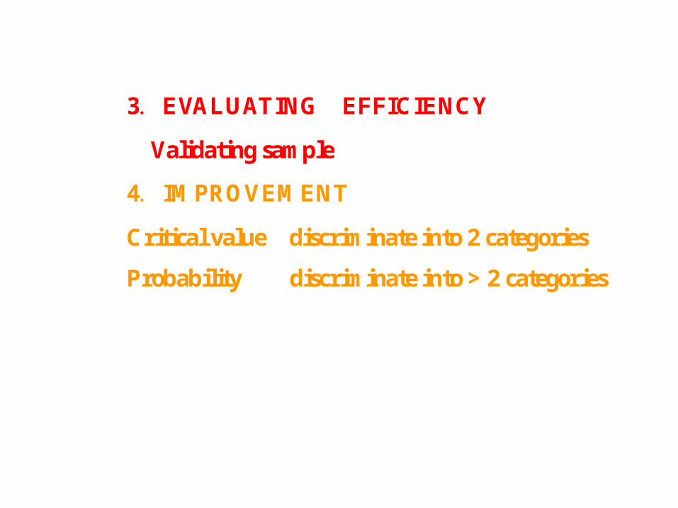
3．EVALUATING EFFICIENCY

Validating sample

4．IMPROVEMENT

Critical value discriminate into 2 categories

Probability discriminate into > 2 categories

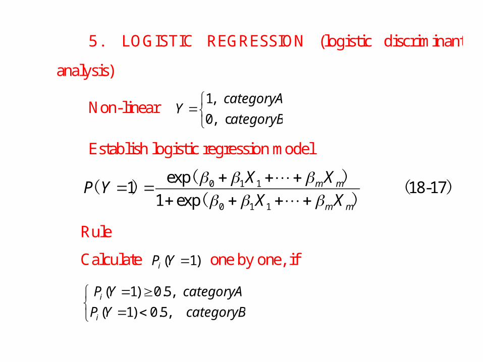
5 ． LOGISTIC REGRESSION (logistic discriminant

analysis)

Non-linear

ategoryB

categoryAY

c ,0

,1

Establish logistic regression model

0 1 1

0 1 1

exp1 18-17

1 expm m

m m

X XP Y

X X

（ ）（ ） （ ）

（ ）

Rule

Calculate )1( YPi one by one, if

categoryBYP

categoryAYP

i

i

,5.0)1(

,5.0)1(

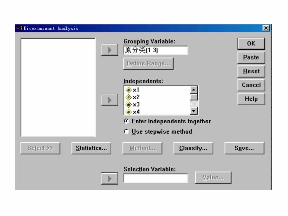
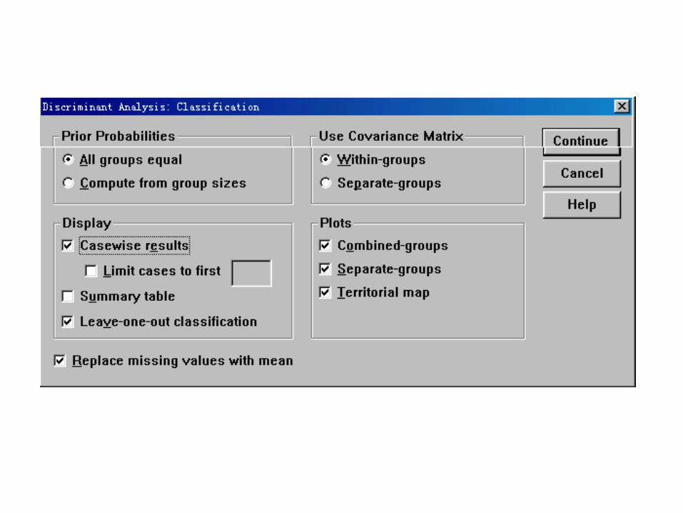
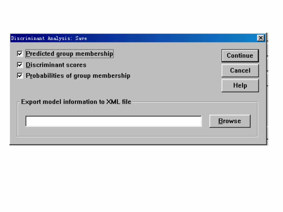
SPSS practice:

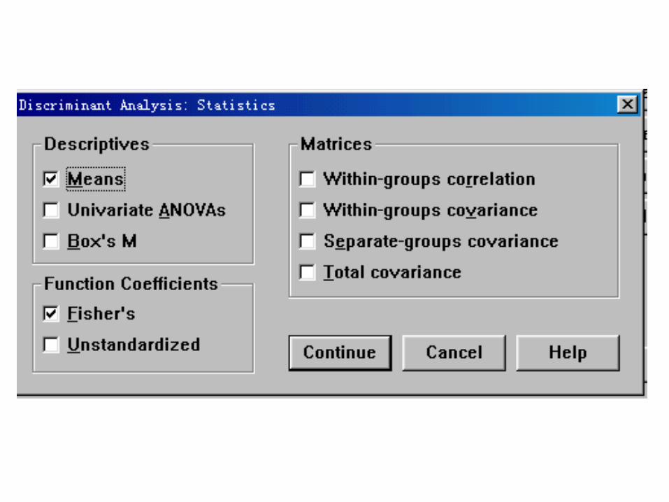
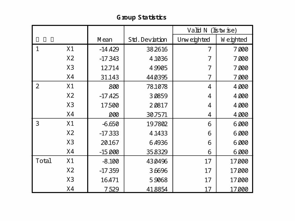
Group Statistics

-14.429 38.2616 7 7.000

-17.343 4.1036 7 7.000

12.714 4.9905 7 7.000

31.143 44.0395 7 7.000

.800 78.1078 4 4.000

-17.425 3.0859 4 4.000

17.500 2.0817 4 4.000

.000 30.7571 4 4.000

-6.650 19.7802 6 6.000

-17.333 4.1433 6 6.000

20.167 6.4936 6 6.000

-15.000 35.8329 6 6.000

-8.100 43.0496 17 17.000

-17.359 3.6696 17 17.000

16.471 5.9068 17 17.000

7.529 41.8854 17 17.000

X1

X2

X3

X4

X1

X2

X3

X4

X1

X2

X3

X4

X1

X2

X3

X4

原分类1

2

3

Total

Mean Std. Deviation Unweighted Weighted

Valid N (listwise)

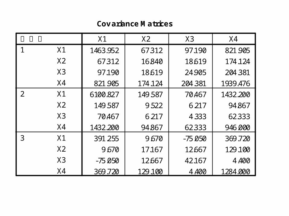
Covariance Matrices

1463.952 67.312 97.190 821.905

67.312 16.840 18.619 174.124

97.190 18.619 24.905 204.381

821.905 174.124 204.381 1939.476

6100.827 149.587 70.467 1432.200149.587 9.522 6.217 94.867

70.467 6.217 4.333 62.333

1432.200 94.867 62.333 946.000

391.255 9.670 -75.050 369.720

9.670 17.167 12.667 129.100

-75.050 12.667 42.167 4.400

369.720 129.100 4.400 1284.000

X1

X2

X3

X4

X1

X2

X3

X4

X1

X2

X3

X4

原分类1

2

3

X1 X2 X3 X4

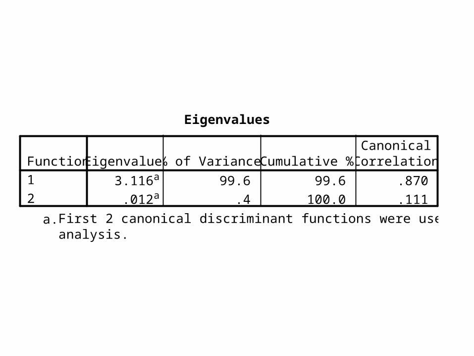
Eigenvalues

3.116a 99.6 99.6 .870

.012a .4 100.0 .111

Function1

2

Eigenvalue % of Variance Cumulative %CanonicalCorrelation

First 2 canonical discriminant functions were used in theanalysis.

a.

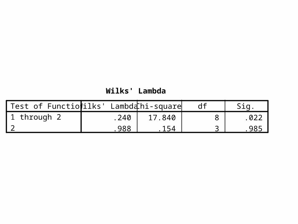
Wilks' Lambda

.240 17.840 8 .022

.988 .154 3 .985

Test of Function(s)1 through 2

2

Wilks' Lambda Chi-square df Sig.

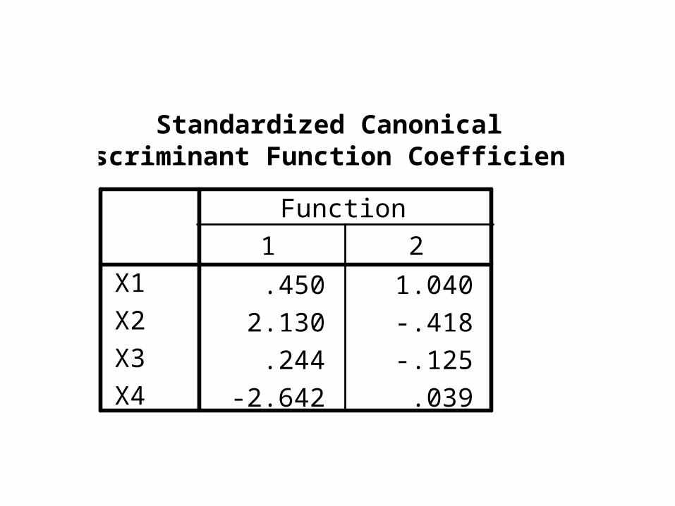
Standardized CanonicalDiscriminant Function Coefficients

.450 1.040

2.130 -.418

.244 -.125

-2.642 .039

X1

X2

X3

X4

1 2

Function

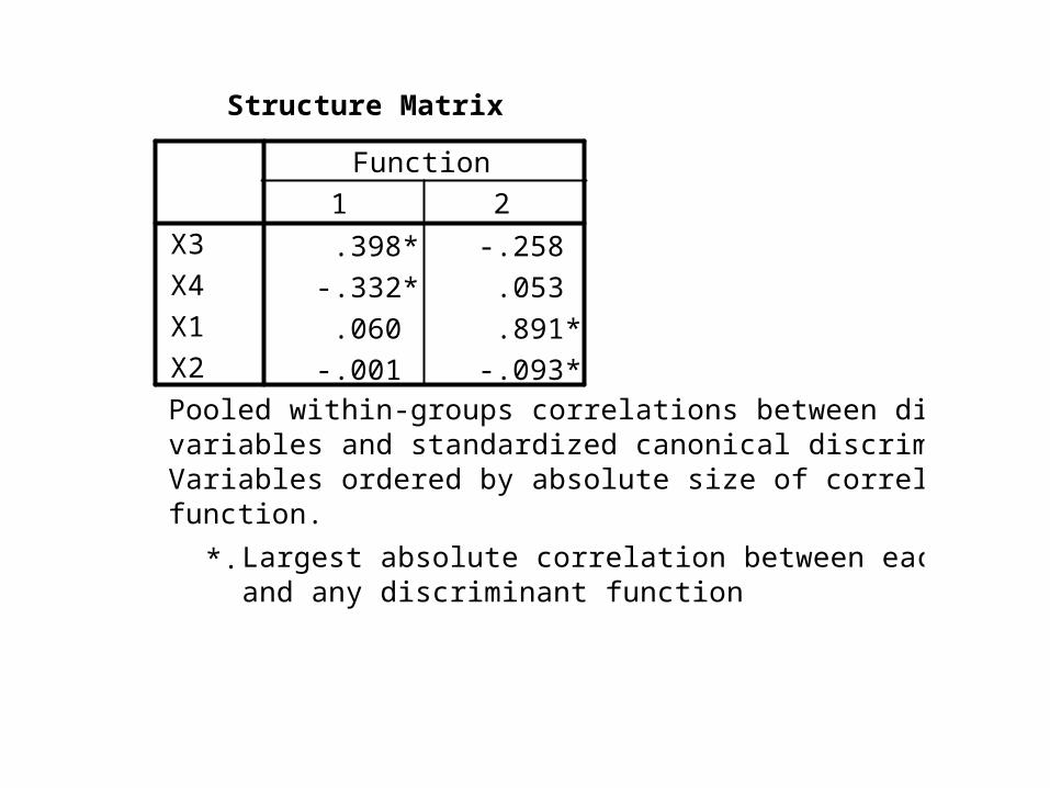
Structure Matrix

.398* -.258

-.332* .053

.060 .891*

-.001 -.093*

X3

X4

X1

X2

1 2

Function

Pooled within-groups correlations between discriminatingvariables and standardized canonical discriminant functions Variables ordered by absolute size of correlation withinfunction.

Largest absolute correlation between each variableand any discriminant function

*.

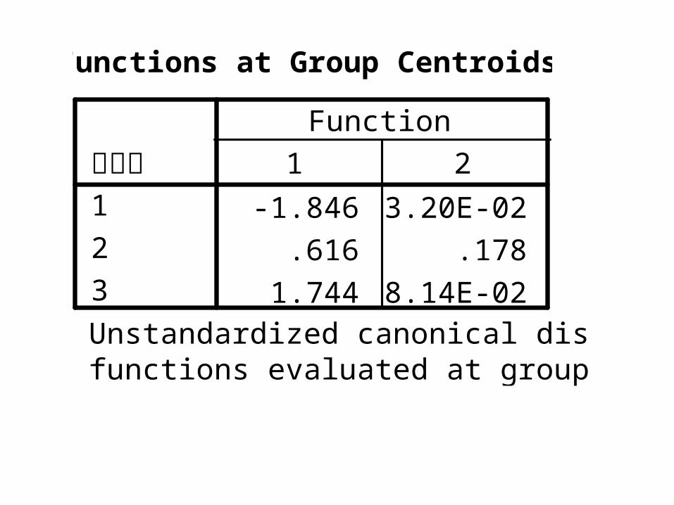
Functions at Group Centroids

-1.846 -3.20E-02

.616 .178

1.744 -8.14E-02

原分类1

2

3

1 2

Function

Unstandardized canonical discriminantfunctions evaluated at group means

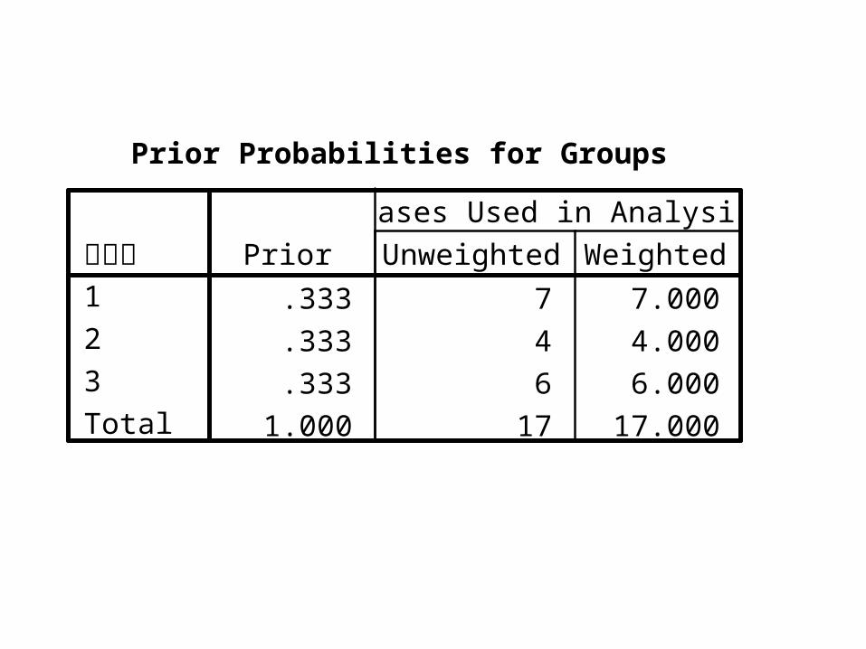
Prior Probabilities for Groups

.333 7 7.000

.333 4 4.000

.333 6 6.000

1.000 17 17.000

原分类1

2

3

Total

Prior Unweighted Weighted

Cases Used in Analysis

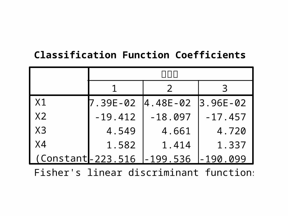
Classification Function Coefficients

-7.39E-02 -4.48E-02 -3.96E-02

-19.412 -18.097 -17.457

4.549 4.661 4.720

1.582 1.414 1.337

-223.516 -199.536 -190.099

X1

X2

X3

X4

(Constant)

1 2 3

原分类

Fisher's linear discriminant functions

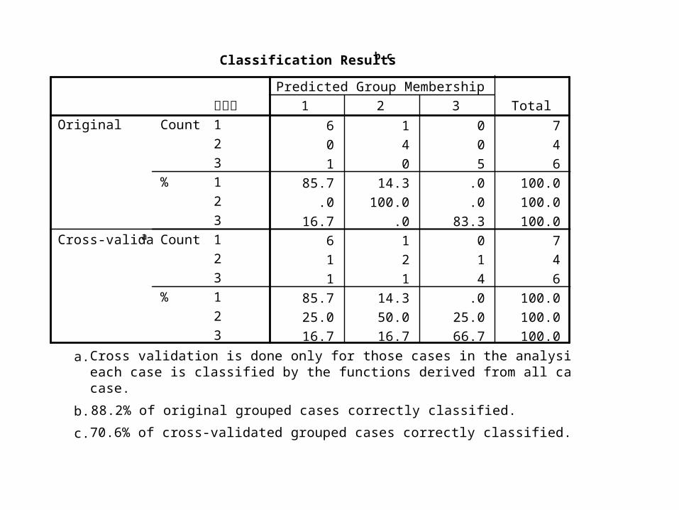
Classification Resultsb,c

6 1 0 7

0 4 0 4

1 0 5 6

85.7 14.3 .0 100.0

.0 100.0 .0 100.0

16.7 .0 83.3 100.0

6 1 0 7

1 2 1 4

1 1 4 6

85.7 14.3 .0 100.0

25.0 50.0 25.0 100.0

16.7 16.7 66.7 100.0

原分类1

2

3

1

2

3

1

2

3

1

2

3

Count

%

Count

%

Original

Cross-validateda

1 2 3

Predicted Group Membership

Total

Cross validation is done only for those cases in the analysis. In cross validation,each case is classified by the functions derived from all cases other than thatcase.

a.

88.2% of original grouped cases correctly classified.b.

70.6% of cross-validated grouped cases correctly classified.c.

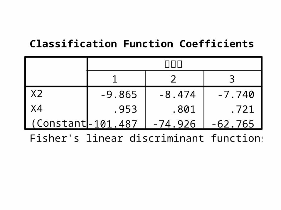
Classification Function Coefficients

-9.865 -8.474 -7.740

.953 .801 .721

-101.487 -74.926 -62.765

X2

X4

(Constant)

1 2 3

原分类

Fisher's linear discriminant functions

Classification Resultsb,c

7 0 0 7

0 4 0 4

1 0 5 6

100.0 .0 .0 100.0

.0 100.0 .0 100.0

16.7 .0 83.3 100.0

6 1 0 7

0 3 1 4

1 0 5 6

85.7 14.3 .0 100.0

.0 75.0 25.0 100.0

16.7 .0 83.3 100.0

原分类1

2

3

1

2

3

1

2

3

1

2

3

Count

%

Count

%

Original

Cross-validateda

1 2 3

Predicted Group Membership

Total

Cross validation is done only for those cases in the analysis. In cross validation,each case is classified by the functions derived from all cases other than thatcase.

a.

94.1% of original grouped cases correctly classified.b.

82.4% of cross-validated grouped cases correctly classified.c.