non-sparse multiple kernel fisher discriminant analysis

Journal of Machine Learning Research 13 (2012) 607-642 Submitted 3/11; Revised 10/11; Published 3/12

Non-Sparse Multiple Kernel Fisher Discriminant Analysis

Fei Yan [email protected]

Josef Kittler [email protected]

Krystian Mikolajczyk [email protected]

Atif Tahir [email protected]

Centre for Vision, Speech and Signal ProcessingUniversity of SurreyGuildford, Surrey, United Kingdom, GU2 7XH

Editor: Soren Sonnenburg, Francis Bach, Cheng Soon Ong

AbstractSparsity-inducing multiple kernel Fisher discriminant analysis (MK-FDA) has been studied in theliterature. Building on recent advances in non-sparse multiple kernel learning (MKL), we proposea non-sparse version of MK-FDA, which imposes a generalℓp norm regularisation on the kernelweights. We formulate the associated optimisation problemas a semi-infinite program (SIP), andadapt an iterative wrapper algorithm to solve it. We then discuss, in light of latest advances in MKLoptimisation techniques, several reformulations and optimisation strategies that can potentially leadto significant improvements in the efficiency and scalability of MK-FDA. We carry out extensiveexperiments on six datasets from various application areas, and compare closely the performanceof ℓp MK-FDA, fixed norm MK-FDA, and several variants of SVM-basedMKL (MK-SVM). Ourresults demonstrate thatℓp MK-FDA improves upon sparse MK-FDA in many practical situations.The results also show that on image categorisation problems, ℓp MK-FDA tends to outperform itsSVM counterpart. Finally, we also discuss the connection between (MK-)FDA and (MK-)SVM,under the unified framework of regularised kernel machines.

Keywords: multiple kernel learning, kernel fisher discriminant analysis, regularised least squares,support vector machines

1. Introduction

Since their introduction in the mid-1990s, kernel methods (Scholkopf and Smola, 2002; Shawe-Taylor and Cristianini, 2004) have proven successful for many machinelearning problems, forexample, classification, regression, dimensionality reduction, clustering. Representative methodssuch as support vector machine (SVM) (Vapnik, 1999; Shawe-Taylorand Cristianini, 2004), kernelFisher discriminant analysis (kernel FDA) (Mika et al., 1999; Baudat and Anouar, 2000), kernelprincipal component analysis (kernel PCA) (Scholkopf et al., 1999) have been reported to producestate-of-the-art performance in numerous applications. Kernel methodswork by embedding dataitems in an input space (vector, graph, string, etc.) into a feature space, and applying linear methodsin the feature space. This embedding is defined implicitly by specifying an innerproduct for thefeature space via a symmetric positive semidefinite (PSD) kernel function.

It is well recognised that in kernel methods, the choice of kernel function is critically important,since it completely determines the embedding of the data in the feature space. Ideally, this em-bedding should be learnt from training data. In practice, a relaxed version of this very challenging

c©2012 Fei Yan, Josef Kittler, Krystian Mikolajczyk and Atif Tahir.

YAN , K ITTLER, M IKOLAJCZYK AND TAHIR

problem is often considered: given multiple kernels capturing different “views” of the problem, howto learn an “optimal” combination of them. Among several others (Cristianini et al., 2002; Chapelleet al., 2002; Bousquet and Herrmann, 2003; Ong et al., 2003), Lanckriet et al. (2002, 2004) are oneof the pioneering works for this multiple kernel learning (MKL) problem.

Lanckriet et al. (2002, 2004) study a binary classification problem, andtheir key idea is tolearn a linear combination of a given set of base kernels by maximising the margin between thetwo classes or by maximising kernel alignment. More specifically, suppose one is givenn m×msymmetric PSD kernel matricesK j , j = 1, · · · ,n, andm class labelsyi ∈ {1,−1}, i = 1, · · · ,m. Alinear combination of then kernels under anℓ1 norm constraint is considered:

K =n

∑j=1

β jK j , β ≥ 0, ‖β‖1 = 1,

whereβ= (β1, · · · ,βn)T ∈R

n, and0 is themdimensional vector of zeros. Geometrically, taking thesum of kernels can be interpreted as taking the Cartesian product of the associated feature spaces.Different scalings of the feature spaces lead to different embeddings of the data in the compositefeature space. The goal of MKL is then to learn the optimal scaling of the feature spaces, such thatthe “separability” of the two classes in the composite feature space is maximised.

Lanckriet et al. (2002, 2004) propose to use the soft margin of SVM asa measure of separa-bility, that is, to learnβ by maximising the soft margin between the two classes. One of the mostcommonly used formulations of the resulting MKL problem is the following saddle point problem:

maxβ

minα

−yTα+12

n

∑j=1

αTβ jK jα (1)

s.t. 1Tα= 0, 0≤ yTα≤C1, β ≥ 0, ‖β‖1 ≤ 1,

whereα ∈ Rm, 1 is themdimensional vector of ones,y is themdimensional vector of class labels,

C is a parameter controlling the trade-off between regularisation and empiricalerror, andK j(xi ,xi′)

is the dot product of theith and thei′th training examples in thej th feature space. Note that inEquation (1), we have replaced the constraint‖β‖1 = 1 by ‖β‖1 ≤ 1, which can be shown to haveno effect on the solution of the problem, but allows for an easier generalisation.

Several alternative MKL formulations have been proposed (Lanckrietet al., 2004; Bach andLanckriet, 2004; Sonnenburg et al., 2006; Zien and Ong, 2007; Rakotomamonjy et al., 2008). Theseformulations essentially solve the same problem as Equation (1), and differ only in the optimisa-tion techniques used. The original semi-definite programming (SDP) formulation (Lanckriet et al.,2004) becomes intractable whenm is in the order of thousands, while the semi-infinite linear pro-gramming (SILP) formulation (Sonnenburg et al., 2006) and the reduced gradient descent algorithm(Rakotomamonjy et al., 2008) can deal with much larger problems.

Of particular interest to this article is the SILP formulation in Sonnenburg et al.(2006). Theauthors propose to use a technique called column generation to solve the SILP, which involvesdividing a SILP into an inner subproblem and an outer subproblem, and alternating between solvingthe two subproblems until convergence. A straightforward implementation of column generationleads to a conceptually very simple wrapper algorithm, where finding the optimalα in the innersubproblem corresponds to solving a standard binary SVM. This means the wrapper algorithm cantake advantage of existing efficient SVM solvers, and can be reasonablyfast for medium-sized

608

NON-SPARSEMULTIPLE KERNEL FISHER DISCRIMINANT ANALYSIS

problems already. However, as pointed out by Sonnenburg et al. (2006), solving the whole SVMproblem to a high precision is unnecessary and therefore wasteful when the variableβ in the outersubproblem is still far from the global optimum.

To remedy this, Sonnenburg et al. (2006) propose to optimiseα andβ in an interleaved manner,by incorporating chunking (Joachims, 1988) into the inner subproblem. The key idea of chunking,and more generally decomposition techniques for SVM, is to freeze all but asmall subset ofα, andsolve only a small-sized subproblems of the SVM dual in each iteration. The resulting interleavedalgorithm in Sonnenburg et al. (2006) avoids the wasteful computation of the whole SVM dual, andas a result has an improved efficiency over the wrapper algorithm. Moreover, with the interleavedalgorithm, only columns of the kernel matrices that correspond to the “active” dual variables needto be loaded into memory, extending MKL’s applicability to large scale problems.

The learning problem in Equation (1) imposes anℓ1 regularisation on the kernel weights. It hasbeen known thatℓ1 norm regularisation tends to produce sparse solutions (Ratsch, 2001), whichmeans during the learning most kernels are assigned zero weights. Conventionally, sparsity isfavoured mainly for two reasons: it offers a better interpretability, and thetest process is moreefficient with sparse kernel weights. However, sparsity is not alwaysdesirable, since the informa-tion carried in the zero-weighted kernels is lost. In Kloft et al. (2008) andCortes et al. (2009),non-sparse versions of MKL are proposed, where anℓ2 norm regularisation is imposed instead ofℓ1 norm. Kloft et al. (2009, 2011) later extended their work to use a general ℓp (p≥ 1) norm regu-larisation. To solve the associated optimisation problem, Kloft et al. (2011) propose extensions ofthe wrapper and the interleaved algorithms in Sonnenburg et al. (2006) respectively. Experiments inKloft et al. (2008, 2009, 2011) show that the regularisation norm contributes significantly to the per-formance of MKL, and confirm that in general a smaller regularisation norm produces more sparsekernel weights.

Although many of the above references discuss general loss functions(Lanckriet et al., 2004;Sonnenburg et al., 2006; Kloft et al., 2011), they have mainly been focusing on the binary hingeloss. In this sense, the corresponding MKL algorithms are essentially binary multiple kernel sup-port vector machines (MK-SVMs). In contrast to SVM, which maximises the soft margin, Fisherdiscriminant analysis (FDA) (Fisher, 1936) maximises the ratio of projected between and withinclass scatters. Since its introduction in the 1930s, FDA has stood the test of time. Equipped recentlywith kernelisation (Mika et al., 1999; Baudat and Anouar, 2000) and efficient implementation (Caiet al., 2007), FDA has established itself as a strong competitor of SVM. In many comparative stud-ies, FDA is reported to offer comparable or even better performance thanSVM (Mika, 2002; Caiet al., 2007; Ye et al., 2008).

In Kim et al. (2006) and Ye et al. (2008), a multiple kernel FDA (MK-FDA)is introduced, wherean ℓ1 norm is used to regularise the kernel weights. As in the case ofℓ1 MK-SVM, ℓ1 MK-FDAtends to produce sparse selection results, which may lead to a loss of information. In this paper,we extend the work of Kim et al. (2006) and Ye et al. (2008) to a generalℓp norm regularisation bybringing latest advances in non-sparse MKL to MK-FDA. Our contributioncan be summarised asfollows:

• We provide a SIP formulation ofℓp MK-FDA for both binary and multiclass problems, andadapt the wrapper algorithm in Sonnenburg et al. (2006) to solve it. By considering recentadvances in large scale MKL techniques, we also discuss several strategies that could signifi-cantly improve the efficiency and scalability of the wrapper-basedℓp MK-FDA. (Section 2)

609


• We carry out extensive experiments on six datasets, including one synthetic dataset, fourobject and image categorisation benchmarks, and one computational biologydataset. Weconfirm that as in the case ofℓp MK-SVM, in ℓp MK-FDA, a smaller regularisation norm ingeneral leads to more sparse kernel weights. We also show that by selecting the regularisationnorm p on an independent validation set, the “intrinsic sparsity” of the given set of basekernels can be learnt. As a result, using the learnt optimal normp in ℓp MK-FDA offersbetter performance than fixed norm MK-FDAs. (Section 3)

• We compare closely the performance ofℓp MK-FDA and that of several variants ofℓp MK-SVM, and show that on object and image categorisation datasets,ℓp MK-FDA has a smallbut consistent edge. In terms of efficiency, our wrapper-basedℓp MK-FDA is comparableto the interleavedℓp MK-SVM on small/medium sized binary problems, but can be sig-nificantly faster on multiclass problems. When compared against recently proposed MKLtechniques that define the state-of-the-art, such as SMO-MKL (Vishwanathan et al., 2010)and OBSCURE (Orabona et al., 2010), our MK-FDA also compares favourably or similarly.(Section 3)

• Finally, we discuss the connection between (MK-)FDA and (MK-)SVM, from the perspec-tives of both loss function and version space, under the unified framework of regularisedkernel machines. (Section 4)

Essentially, our work builds on Sonnenburg et al. (2006), Ye et al. (2008) and Kloft et al. (2011).However, we believe the empirical findings of this paper, especially the onethat (MK-)FDA tendsto outperform (MK-)SVM on image categorisation datasets, is important, given that SVM and SVMbased MKL are widely accepted as the state-of-the-art classifier in most image categorisation sys-tems. Finally, note that preliminary work to this article has been published previously as conferencepapers (Yan et al., 2009b,a, 2010). The aim of this article is to consolidate theresults into an in-tegrated and comprehensive account and to provide more experimental results in support of theproposed methodology.

2. ℓp Norm Multiple Kernel FDA

In this section we first present ourℓp regularised MK-FDA for binary problems and then for multi-class problems. In both cases, we first give problem formulation, then solve the associated optimi-sation problem using a wrapper algorithm. Towards the end of this section, we also discuss severalpossible improvements over the wrapper algorithm in terms of time and memory complexity, inlight of recent advances in MKL optimisation techniques.

2.1 Binary Classification

Given a binary classification problem withm training examples, our goal is to learn the optimalkernel weightsβ ∈ R

n for a linear combination ofn base kernels under theℓp (p≥ 1) constraint:

K =n

∑j=1

β jK j , β j ≥ 0, ‖β‖pp ≤ 1,

where thep≥ 1 requirement is to ensure that the triangle inequality is satisfied and‖ ·‖p is a norm.We define optimality in terms of the class separation criterion of FDA, that is, the learnt kernel

610


weightsβ are optimal, if the ratio of the projected between and within class scatters is maximised.In this paper we assume each kernel is centred in its feature space. Centring can be performedimplicitly (Scholkopf et al., 1999) byK j = PK jP, whereP is them×m centring matrix defined asP= I − 1

m1·1T , K j is the uncentred kernel matrix, andI is them×m identity matrix.Let m+ be the number of positive training examples, andm− = m−m+ be that of negative

training examples. For a given kernelK, let φ(x+i ) be theith positive training point in the implicitfeature space associated withK, φ(x−i ) be theith negative training point in the feature space. Herex+i andx−i can be thought of as training examples in some input space, andφ is the mapping to thefeature space. Also letµ+ andµ− be the centroids of the positive examples and negative examplesin the feature space, respectively:

µ+ =1

m+

m+

∑i=1

φ(x+i ), µ− =1

m−

m−

∑i=1

φ(x−i ).

The within class covariance matrices of the two classes are:

C+ =1

m+

m+

∑i=1

(

φ(x+i )−µ+

)(

φ(x+i )−µ+

)T

,

C− =1

m−

m−

∑i=1

(

φ(x−i )−µ−

)(

φ(x−i )−µ−

)T

.

The between class scatterSB and within class scatterSw are then defined as:

SB =m+m−

m(µ+−µ−)(µ+−µ−)T , (2)

SW = m+C++m−C−.

The objective of single kernel FDA is to find the projection directionw in the feature space that

maximiseswTSBwwTSWw , or equivalently,

wT mm+m− SBwwTSTw , whereST = SB+SW is the total scatter matrix. In

practice a regularised objective function

JFDA(w) =wT m

m+m− SBwwT(ST +λI)w

(3)

is maximised to improve generalisation and numerical stability (Mika, 2002), where λ is a smallpositive number.

From Theorem 2.1 of Ye et al. (2008), for a given kernelK, the maximal value of Equation (3)is:

J∗FDA = aTa−aT(

I +1λ

K

)−1

a, (4)

where

a=

(

1m+

, · · · ,1

m+,−1m−

, · · · ,−1m−

)T

∈ Rm

contains the centred labels. On the other hand, Lemma 2.1 of Ye et al. (2008)states that thew thatmaximises Equation (3) also minimises the following regularised least squares (RLS):

JRLS(w) = ‖φT(X)w−a‖2+λ‖w‖2, (5)

611


and the minimum of Equation (5) is given by:

J∗RLS= aT(

I +1λ

K

)−1

a. (6)

In Equation (5),φ(X) = (φ(x+1 ), · · · ,φ(x+m+),φ(x−1 ), · · · ,φ(x

−m−)) are the (centred) training data in

the feature space such thatφ(X)Tφ(X) = K.Due to strong duality, the minimal value of Equation (5) is equal to the maximal valueof its

Lagrangian dual problem, that is,

J∗RLS= maxα

aTα−14αTα+

14λ

αTKα,

or equivalently

J∗RLS=−minα

(

−aTα+14αTα+

14λ

αTKα

)

, (7)

whereα ∈ Rm. By combining Equation (4), Equation (6) and Equation (7), it follows that the

maximal value of the FDA objective in Equation (3) is given by:

J∗FDA = aTa+minα

(

−aTα+14αTα+

14λ

αTKα

)

. (8)

Now instead of a fixed single kernel, consider the case where the kernelK can be chosen fromlinear combinations of a set of base kernels. The kernel weights must be regularised somehow tomake sure Equation (8) remains meaningful and does not become arbitrarilylarge. In this paper, wepropose to impose anℓp regularisation on the kernel weights for anyp≥ 1, following Kloft et al.(2009, 2011):

K =

{

K =n

∑j=1

β jK j : β ≥ 0,‖β‖pp ≤ 1

}

. (9)

Combining Equation (9) and Equation (8), and dropping the unimportant constantaTa, it can beshown that the optimalK ∈ K maximising Equation (4) is found by solving:

maxβ

minα

−aTα+14αTα+

14λ

n

∑j=1

αTβ jK jα (10)

s.t. β ≥ 0, ‖β‖pp ≤ 1.

Note that putting anℓp constraint onβ or penalizingw by anℓ2,r block norm are equivalent withp = r/(2− r) (Szafranski et al., 2008). Whenp = 1, we have theℓ1 MK-FDA discussed in Yeet al. (2008); whilep= ∞ leads tor = 2, and MK-FDA reduces to standard single kernel FDA withunweighted concatenation of base feature spaces. In this paper, however, we are interested in thegeneral case of anyp≥ 1.

Equation (10) is an optimisation problem with a quadratic objective and a general pth orderconstraint. We borrow the idea fromℓp MK-SVM (Kloft et al., 2009, 2011) and use second orderTaylor expansion to approximate the norm constraint:

‖β‖pp ≈

p(p−1)2

n

∑j=1

βp−2j β2

j −n

∑j=1

p(p−2)βp−1j β j +

p(p−3)2

+1 := ν(β), (11)

612


whereβ j is the current estimate ofβ j in an iterative process, which will be explained in more detailshortly. Substituting Equation (11) into Equation (10), we arrive at the binary ℓp MK-FDA saddlepoint problem:

maxβ

minα

−aTα+14αTα+

14λ

n

∑j=1

αTβ jK jα (12)

s.t. β ≥ 0, ν(β)≤ 1.

In Sonnenburg et al. (2006), the authors propose to transform a saddle point problem similarto Equation (12) to a semi-infinite program (SIP). A SIP is an optimisation problem with a finitenumber of variablesx ∈ R

d on a feasible set described by infinitely many constraints (Hettich andKortanek, 1993):

minx

f (x) s.t. g(x,u)≥ 0 ∀u∈U,

whereU is an infinite index set. Following the similar arguments as in Sonnenburg et al. (2006)and Ye et al. (2008), we show in Theorem 1 that the saddle point problemin Equation (12) can alsobe transformed into a SIP.

Theorem 1 Given a set of n kernel matrices K1, · · · ,Kn, the kernel weightsβ that optimise Equa-tion (12)are given by solving the following SIP problem:

maxθ,β

θ (13)

s.t. −aTα+14αTα+

14λ

n

∑j=1

αTβ jK jα≥ θ ∀α ∈ Rm, β ≥ 0, ν(β)≤ 1.

Proof Letα∗ be the optimal solution to the saddle point problem in Equation (12). By defining

θ∗ :=−aTα∗+14α∗Tα∗+

14λ

n

∑j=1

α∗Tβ jK jα∗

as the minimum objective value achieved byα∗, we have

−aTα+14αTα+

14λ

n

∑j=1

αTβ jK jα≥ θ∗

∀α ∈ Rm. Now define

θ = minα

−aTα+14αTα+

14λ

n

∑j=1

αTβ jK jα

and substitute it into Equation (12), the theorem is proved.

We adapt the wrapper algorithm in Sonnenburg et al. (2006) to solve the SIP in Equation (13).This algorithm is based on the column generation technique, where the basic idea is to divide a SIPinto an inner subproblem and an outer subproblem. The algorithm alternatesbetween solving the

613


Algorithm 1 A wrapper algorithm for solving the binaryℓp MK-FDA SIP in Equation (13)

Input: K1, · · · ,Kn, a, θ(1) =−∞, β(1)j = n−1/p∀ j, ε.

Output: Learnt kernel weightsβ = (β(t)1 , · · · ,β(t)

n )T .1: for t = 1, · · · do2: Computeα(t) in Equation (15);3: ComputeS(t) =−aTα(t)+ 1

4α(t)Tα(t)+ 1

4λ ∑nj=1α

(t)Tβ(t)j K jα

(t);

4: if |1− S(t)

θ(t) | ≤ ε then5: break;6: end if7: Compute{θ(t+1),β(t+1)} in Equation (16), whereν(β) is defined as in Equation (11) with

β = β(t);8: end for

two subproblems until convergence. At stept, the inner subproblem (α step) identifies the constraintthat maximises the constraint violation for{θ(t),β(t)}:

α(t) := argminα

−aTα+14αTα+

14λ

n

∑j=1

αTβ(t)j K jα. (14)

Note that the program in Equation (14) is nothing but the single kernel FDA/RLS dual problemusing the current estimateβ(t) as kernel weights. Observing that Equation (14) is an unconstrainedquadratic program,α(t) is obtained by solving the following linear system (Ye et al., 2008):

(

12

I +12λ

n

∑j=1

β(t)j K j

)

α(t) = a. (15)

If α(t) satisfies constraint−aTα(t)+ 14α

(t)Tα(t)+ 14λ ∑n

j=1α(t)Tβ(t)

j K jα(t) ≥ θ(t) then{θ(t),β(t)} is

optimal. Otherwise, the constraint is added to the set of constraints and the algorithm proceeds tothe outer subproblem of stept.

The outer subproblem (β step) is also called the restricted master problem. At stept, it computesthe optimal{θ(t+1),β(t+1)} in Equation (13) for a restricted subset of constraints:

{θ(t+1),β(t+1)}= argmaxθ,β

θ (16)

s.t. −aTα(r)+14α(r)Tα(r)+

14λ

n

∑j=1

α(r)Tβ jK jα(r) ≥ θ ∀r = 1, · · · , t, β ≥ 0, ν(β)≤ 1.

When p= 1, ν(β) ≤ 1 reduces to a linear constraint. As a result, Equation (16) becomes a linearprogram (LP) and theℓp MK-FDA reduces to theℓ1 MK-FDA in Ye et al. (2008). Whenp > 1,Equation (16) is a quadratically constrained linear program (QCLP) with one quadratic constraintν(β)≤ 1 andt +n linear constraints. This can be solved by off-the-shelf optimisation tools such asMosek.1 Note that at timet, ν(β) is defined as in Equation (11) withβ = β(t), that is, the currentestimate ofβ.

1. Mosek optimisation toolbox can be found athttp://www.mosek.com .

614


Normalised maximal constraint violation is used as a convergence criterion. The algorithmstops when|1− S(t)

θ(t) | ≤ ε, whereS(t) := −aTα(t)+ 14α

(t)Tα(t)+ 14λ ∑n

j=1α(t)Tβ(t)

j K jα(t) andε is a

pre-defined accuracy parameter. This iterative wrapper algorithm forsolving the binaryℓp MK-FDA SIP is summarised in Algorithm 1. It is a special case of a set of semi-infinite programmingalgorithms known as exchange methods, which are guaranteed to converge (Hettich and Kortanek,1993). Finally, note that in line 4 of Algorithm 1,β(t+1) can also be solved using the analyticalupdate in Kloft et al. (2011) that is adapted to FDA. However, in practice we notice that for MK-FDA, such an analytical update tends to be numerically unstable whenp is close to 1.

2.2 Multiclass Classification

In this section we consider the multiclass case. Letc be the number of classes, andmk be the numberof training examples in thekth class. In multiclass FDA, the following objective is commonlymaximised (Ye et al., 2008):

JMC−FDA(W) = trace

(

(

WT(ST +λI)W)−1

WTSBW

)

, (17)

whereW is the projection matrix, the within class scatterSW is defined in a similar way as inEquation (2) but withc classes, and the between class scatter isSB = φ(X)HHTφ(X)T , whereφ(X) = (φ(x1),φ(x2), · · · ,φ(xm)) is the set ofm training examples in the feature space, andH =(h1,h2, · · · ,hc) is anm×c matrix withhk = (h1k, · · · ,hmk)

T and

hik =

{ √

mmk

−√mk

m if yi = k

−√mk

m if yi 6= k.(18)

Similar to the binary case, using duality theory and the connection between FDAand RLS, Yeet al. (2008) show that the maximal value of Equation (17) is given by (up toan additive constantdetermined by the labels):

J∗MC−FDA ∼ minαk

c

∑k=1

(

−hTk αk+

14αT

k αk+14λ

αTk Kαk

)

,

whereαk ∈ Rm for k = 1, · · · ,c. When choosing from linear combinations of a set of base kernels

with kernel weights regularised with anℓp norm, the optimal kernel weights are given by:

maxβ

minαk

c

∑k=1

(

−hTk αk+

14αT

k αk+14λ

n

∑j=1

αTk β jK jαk

)

(19)

s.t. β ≥ 0, ‖β‖pp ≤ 1.

We use again second order Taylor expansion to approximate the norm constraint and arrive at themulticlassℓp MK-FDA saddle point problem:

maxβ

minαk

c

∑k=1

(

−hTk αk+

14αT

k αk+14λ

n

∑j=1

αTk β jK jαk

)

s.t. β ≥ 0, ν(β)≤ 1,

615


Algorithm 2 A wrapper algorithm for solving the multiclassℓp MK-FDA SIP in Equation (20)

Input: K1, · · · ,Kn, a, θ(1) =−∞, β(1)j = n−1/p∀ j, ε.

Output: Learnt kernel weightsβ = (β(t)1 , · · · ,β(t)

n )T .1: for t = 1, · · · do2: Computeα(t)

k in Equation (21);

3: ComputeS(t) = ∑ck=1

(

−hTk α

(t)k + 1

4α(t)Tk α

(t)k + 1

4λ ∑nj=1α

(t)Tk β(t)

j K jα(t)k

)

;

4: if |1− S(t)

θ(t) | ≤ ε then5: break;6: end if7: Compute{θ(t+1),β(t+1)} in Equation (22), whereν(β) is defined as in Equation (11) with

β = β(t);8: end for

whereν(β) is defined as in Equation (11).Again similar to the binary case, Equation (19) can be reformulated as a SIP:

maxθ,β

θ (20)

s.t.c

∑k=1

(

−hTk αk+

14αT

k αk+14λ

n

∑j=1

αTk β jK jαk

)

≥ θ ∀αk ∈ Rm, β ≥ 0, ν(β)≤ 1,

and the SIP can be solved using a column generation algorithm that is similar to Algorithm 1. Inthe inner subproblem, the only difference is that instead of one linear system, herec linear systemsneed to be solved, one for eachhk:

(

12

I +12λ

n

∑j=1

β(t)j K j

)

α(t)k = hk. (21)

Accordingly, the outer subproblem for computing the optimal{θ(t+1),β(t+1)} is adapted to workwith multiple classes:

(θ(t+1),β(t+1)) = argmaxθ,β

θ (22)

s.t.c

∑k=1

(

−hTk α

(r)k +

14α

(r)Tk α

(r)k +

14λ

n

∑j=1

α(r)Tk β jK jα

(r)k

)

≥ θ ∀r = 1, · · · , t

β ≥ 0, ν(β)≤ 1.

Whenp= 1, Equation (22) reduces to an LP and our formulation reduces to that in Yeet al. (2008).For p> 1, Equation (22) is an QCLP with one quadratic constraint andt +n linear constraints, asin the binary case. The iterative wrapper algorithm for solving the multiclassℓp MK-FDA SIP issummarised in Algorithm 2.

2.3 Addressing Efficiency Issues

In this section we discuss several possible improvements over the wrapper-basedℓp MK-FDAmethod proposed in the previous sections. In particular, we address time and memory complex-ity issues, in light of recent advances in MKL optimisation techniques. We show that by exploiting

616


the equivalence between kernel FDA and least squares SVM (LSSVM)(Suykens and Vandewalle,1999), the interleaved method in Sonnenburg et al. (2006) and Kloft et al. (2011) can be appliedto MK-FDA. Furthermore, we demonstrate that the formulation in Vishwanathanet al. (2010) thattackles directly the MKL dual problem can also be adapted to work with MK-FDA. Both new for-mulations discussed in this section are equivalent to previous ones in terms oflearnt kernel weights,but can potentially lead to significant efficiency improvement. However, notethat we describe thesenew formulations only briefly, and do not show their efficiency in the experiments section and theirimplementation details, since these are not in the main scope of this paper. Note also that in the fol-lowing we focus only on multiclass formulations, as the corresponding binaryones can be derivedin a very similar fashion, or as special cases.

2.3.1 INTERLEAVED OPTIMISATION OF THE SADDLE POINT PROBLEM

We consider the multiclass MKL problem for a general convex loss functionV(ξik,hik):

minw jk,ξik,β

c

∑k=1

(

12

n

∑j=1

||w jk||2

β j+C

m

∑i=1

V(ξik,hik)

)

(23)

s.t.n

∑j=1

wTjkφ j(xi) = ξik, ∀i, ∀k; β ≥ 0; ||β||2p ≤ 1,

wherehik is as defined in Equation (18), and we have replaced the constraint||β||pp ≤ 1 equiva-lently by ||β||2p ≤ 1. WhenV(ξik,hik) is the square lossV(ξik,hik) =

12(ξik −hik)

2, Equation (23)is essentially multiclass multiple kernel regularised least squares (MK-RLS).It can be shown (seeAppendix A for details) that this multiclass MK-RLS can be reformulated as the following saddlepoint problem:

minβ

maxαk

c

∑k=1

(

hTk αk−

12C

αTk αk−

12

n

∑j=1

αTk β jK jαk

)

(24)

s.t. β ≥ 0; ||β||2p ≤ 1.

Making substitutionsαk →C2αk and thenC → 1

λ , it directly follows that the MK-RLS in Equa-tion (24) is equivalent to the MK-FDA in Equation(19). In the previous sections, we proposed touse a conceptually very simple wrapper algorithm to solve it. However, as pointed out in Sonnen-burg et al. (2006) and Kloft et al. (2011), such an algorithm has two disadvantages: solving thewhole single kernel problem in theα step is unnecessary therefore wasteful, and all kernels needto be loaded into memory. These problems, especially the second one, significantly limit the scal-ability of wrapper-based MKL algorithms. For example, 50 kernel matrices of size 20000×20000would usually not fit into memory since they require approximately 149GB of memory (Kloft et al.,2011).

Exploiting the fact that LSSVM, RLS and kernel FDA are equivalent (Rifkin, 2002; Gestel et al.,2002; Keerthi and Shevade, 2003), sequential minimal optimisation (SMO) techniques (Joachims,1988) developed for LSSVM (Keerthi and Shevade, 2003; Lopez and Suykens, 2011) can be em-ployed to remedy these problems. This effectively leads to an interleaved algorithm that is similarto Algorithm 2 in Kloft et al. (2011), but applies to square loss instead of to hinge loss. Such aninterleaved optimisation strategy allows for a very cheap update of a minimal subset of the dual

617


variablesαk in eachα step, without having to have access to the whole kernel matrices, and as aresult extends the applicability of MK-FDA to large scale problems. We omit details of the resultinginterleaved MK-FDA algorithm, the interested reader is referred to Keerthiand Shevade (2003) andLopez and Suykens (2011).

2.3.2 WORKING DIRECTLY WITH THE DUAL

The MK-FDA algorithms considered so far, including the wrapper method and the interleavedmethod, are all based on the intermediate saddle point formulation Equation (24), or equivalently,Equation(19). Recently, a “direct” formulation of MKL was proposed in Vishwanathan et al. (2010),where the idea is to eliminateβ from the saddle point problem, and deal directly with the dual. Con-sider again MKL with a general convex loss, but following Vishwanathan et al. (2010) this time weimpose the norm constraint in the form of Tikhonov regularisation instead ofIvanov regularisation:

minw jk,ξik,β

c

∑k=1

(

12

n

∑j=1

‖w jk‖2

β j+C

m

∑i=1

V(ξik,hik)

)

+µ2‖β‖2

p (25)

s.t.n

∑j=1

wTjkφ j(xi) = ξik, ∀i, ∀k; β ≥ 0.

Note that the two formulations in Equation (25) and Equation (23) are equivalent, in the sense thatfor any givenC there exists aµ (and vice versa) such that the optimal solutions to both problems areidentical (Kloft et al., 2011).

It can be shown (see Appendix B for details) that for the special case of square loss, whichcorresponds to MK-FDA/MK-RLS, the dual of Equation(25) is:

maxαk

c

∑k=1

(

hTk αk−

12C

αTk αk

)

−18µ

∥

∥

∥

∥

( c

∑k=1

αTk K jαk

)n

j=1

∥

∥

∥

∥

2

q, (26)

whereq= pp−1 is the dual norm ofp, and once the optimalαk are found by solving Equation (26),

the kernel weights are given by:

β j =12µ

( n

∑j=1

(c

∑k=1

αTk K jαk)

q)

1q−

1p

(c

∑k=1

αTk K jαk)

qp .

Equation (26) can be viewed as an extension of Equation (9) in Vishwanathan et al. (2010) tomulticlass problems. Another difference is that Equation (9) in Vishwanathanet al. (2010) considersa hinge loss, while Equation (26) is for square loss. Similarly as in Vishwanathan et al. (2010), forany p> 1, Equation (26) can be solved using an SMO type of algorithm, with the updaterule forthe minimal subset of dual variables adapted to work with square loss (Keerthi and Shevade, 2003;Lopez and Suykens, 2011). On the other hand, observing that Equation (26) is an unconstrained op-timisation problem and the objective function is differentiable everywhere for p> 1, an alternativeapproach is the quasi-Newton descent methods, for example, the limited memoryvariant (Liu andNocedal, 1989). In fact, Equation (26) can also be thought of as an extension of the smooth variantof group Lasso considered in Kloft et al. (2011) to multiclass case. Note however that Equation (26)has a term ofℓq norm squared, while the smooth group Lasso formulation in Kloft et al. (2011)has a term ofℓq norm. This is a direct result of the fact that the two formulations use Tikhonovregularisation and Ivanov regularisation overβ, respectively.

618


3. Experiments

In this section we validate the usefulness of the proposedℓp MK-FDA with experimental evidenceon six datasets. The experiments can be divided into four groups:

• We first demonstrate in Section 3.1 and 3.2 the different behaviour of the sparseℓ1 MK-FDAand a non-sparse version of MK-FDA (ℓ2 norm) on synthetic data and the Pascal VOC2008object recognition dataset (Everingham et al., 2008). The goal of these two experiments isto confirm thatℓ1 andℓ2 regularisations indeed lead to sparse and non-sparse kernel weightsrespectively.

• Next in Section 3.3, 3.4 and 3.5 we carry out experiments on another three object and imagecategorisation benchmarks, namely, Pascal VOC2007 (Everingham et al., 2007), Caltech101(Fei-Fei et al., 2006), and Oxford Flower17 (Nilsback and Zisserman,2008). We show thatby selecting the regularisation normp on an independent validation set, the intrinsic sparsityof the given set of base kernels can be learnt. As a result, using the learnt optimal normp inthe proposedℓp MK-FDA offers better performance thanℓ1 or ℓ∞ MK-FDAs. Moreover, wecompare the performance ofℓp MK-FDA and that of several variants ofℓp MK-SVM, andshow that on image categorisation problemsℓp MK-FDA tends to have a small but consistentedge over its SVM counterpart.

• In Section 3.6 we further compareℓp MK-FDA and ℓp MK-SVM on the protein subcellularlocalisation problem studied in Zien and Ong (2007) and Ong and Zien (2008). On this datasetℓp MK-SVM outperformsℓp MK-FDA by a small margin, and the results suggest that giventhe same set of base kernels, the two MKL algorithms may favour slightly different norms.

• Finally, in Section 3.7, the training speed of our wrapper-basedℓp MK-FDA and severalℓp

MK-SVM implementations is analysed empirically on a few small/medium sized problems,where MK-FDA compares favourably or similarly against state-of-the-art MKL techniques.

Among the six datasets used in the experiments, three of them (synthetic, VOC08, VOC07) arebinary problems and the rest (Caltech101, Flower17, Protein) are multiclass ones. In our experi-ments the wrapper-basedℓp MK-FDA is implemented in Matlab with the outer-subproblem solvedusing the Mosek optimisation toolbox. The code of ourℓp MK-FDA implementation is available on-line.2 Once the kernel weights have been learnt, we use a spectral regression based efficient kernelFDA implementation (Cai et al., 2007; Tahir et al., 2009) to compute the optimal projection direc-tions, the code of which is also available online.3 On binary problems, we compareℓp MK-FDAwith two implementations of binaryℓp MK-SVM, namely, MK-SVM Shogun (Sonnenburg et al.,2006, 2010),4 and SMO-MKL (Vishwanathan et al., 2010);5 while on multiclass problems, we com-pareℓp MK-FDA with two variants of multiclassℓp MK-SVM: MK-SVM Shogun and MK-SVMOBSCURE (Orabona et al., 2010; Orabona and Jie, 2011).6 In bothℓp MK-FDA and ℓp MK-SVM

2. The code of ourℓp MK-FDA is available athttp://www.featurespace.org3. The code of spectral regression FDA can be found athttp://www.zjucadcg.cn/dengcai/SR/index.html .4. Version 0.10.0 of the Shogun toolbox, the latest version as of the writing of this paper, can be found athttp:

//www.shogun-toolbox.org .5. The code of SMO-MKL is available athttp://research.microsoft.com/en-us/um/people/manik /code/

SMO-MKL/download.html .6. The code of OBSCURE can be found athttp://dogma.sourceforge.net .

619


Shogun, the stopping thresholdε is set to 10−4 unless stated otherwise. Parameters in MK-SVMOBSCURE and SMO-MKL are set to default values unless stated otherwise.

All kernels used in the experiments have been normalised. For the first fivedatasets, due to thekernel functions used, the kernel matrices are by definition spherically normalised: all data pointslie on the unit hypersphere in the feature space. For the protein localisationdataset, the kernelsare multiplicatively normalised following Ong and Zien (2008) and Kloft et al. (2011) to allowcomparison with Kloft et al. (2011). After normalisation, the kernels are then centred in the featurespaces, as required byℓp MK-FDA. Note thatℓp MK-SVM is not affected by centring. Kernelsused in the experiments (except for those in the simulation and in training speedexperiments) arealso available online.7

3.1 Simulation

We first perform simulation to illustrate the different behaviour ofℓ1 MK-FDA and a special caseof ℓp MK-FDA, namely, the case ofp= 2. We simulate two classes by sampling 100 points fromtwo 2-dimensional Gaussian distributions, 50 points from each. The means of the two distributionsin both dimensions are drawn from a uniform distribution between 1 and 2, and the covariancesof the two distributions are also randomly generated. A radial basis function(RBF) kernel is thenconstructed using these 2-dimensional points. Similarly, 100 test points are sampled from the samedistributions, 50 from each, and an RBF kernel is built for the test points.Kernel FDA is thenapplied to find the best projection direction in the feature space and compute the error rate on thetest set. Figure 1 (a) gives 3 examples of the simulated points. It shows thatdue to the parametersused in the two Gaussian distributions, the two classes are heavily, but not completely, overlapping.As a result, the error rate given by single kernel FDA is around 0.43: slightly better than a randomguess.

The above process of mean/covariance generation, sampling, and kernel building is repeatedntimes, resulting inn training kernels (andn corresponding test kernels). Thesen training kernels,although generated independently, can be thought of as kernels that capture different “views” of asingle binary classification problem. With this interpretation in mind, we applyℓ1 andℓ2 MK-FDAsto learn optimal kernel weights for this classification problem. We vary the number n from 5 to 50at a step size of 5. For each value ofn, ℓ1 andℓ2 MK-FDAs are applied and the resulting errorrates are recorded. This process is repeated 100 time for each value ofn to compute the mean andstandard deviation of error rates. The results for variousn values are plotted in Figure 1 (c).

It is clear in Figure 1 (c) that as the number of kernels increases, the error rates of both methodsdrop. This is expected, since more kernels bring more discriminative information. Another obser-vation is thatℓ1 MK-FDA slightly outperformsℓ2 MK-FDA when the number of kernels is 5, andvice versa when the number of kernels is 10 or 15. When there are 20 kernels, the advantage ofℓ2

MK-FDA becomes clear. As the number of kernels keeps increasing, its advantage becomes moreand more evident.

The different behaviour ofℓ1 andℓ2 MK-FDAs can be explained by the different weights learntfrom them. Two typical examples of such weights, learnt usingn = 5 kernels andn = 30 kernelsrespectively, are plotted in Figure 1 (b). It has been known thatℓ1 norm regularisation tends toproduce sparse solutions (Ratsch, 2001; Kloft et al., 2008). When kernels carry complementaryinformation, this will lead to a loss of information and hence degraded performance. When the

7. The kernels can be downloaded athttp://www.featurespace.org .

620


(a)

(b) (c)

Figure 1: Simulation: (a) Three examples of the two Gaussian distributions. (b) Comparing thekernel weights learnt fromℓ1 MK-FDA and ℓ2 MK-FDA. Left: using 5 kernels. Right:using 30 kernels. (c) Mean and standard deviation of error rates ofℓ1 MK-FDA and ℓ2

MK-FDA using various number of kernels.

number of kernels is sufficiently small, however, this effect does not occur: as can be seen in theleft plot of Figure 1 (b), when there are only 5 kernels, all of them get non-zero weights in bothℓ1

andℓ2 MK-FDAs.As the number of kernels increases, eventually there are enough of themfor the over-selectiveness

of ℓ1 regularisation to exhibit itself. As the right plot of Figure 1 (b) shows, when 30 kernels areused, many of them are assigned zero weights byℓ1 MK-FDA. This leads to a loss of information.By contrast, the weights learnt inℓ2 MK-FDA are non-sparse, hence the better performance. Fi-nally, it is worth noting that the sparsity of learnt kernel weights, which captures the sparsity ofinformation in the kernel set, is not to be confused with the numerical sparsityof the kernel matri-ces. For example, when the RBF kernel function is used, the kernel matrices will not contain anyzero, regardless of the sparsity of kernel weights.

3.2 Pascal VOC2008

In this section, we demonstrate again the different behaviour ofℓ1 andℓ2 MK-FDAs, but this timeon a real world dataset: the Pascal visual object classes (VOC) challenge 2008 development dataset.The VOC challenge provides a yearly benchmark for comparison of object classification methods,with one of the most challenging datasets in the object recognition / image classification community.The VOC2008 development dataset consists of 4332 images of 20 object classes such as aeroplane,cat, person, etc. The dataset is divided into a pre-defined training set with 2111 images and avalidation set with 2221 images. In our experiments, the training set is used for training and thevalidation set for testing. VOC2008 test set is not used as the class labels are not publicly available.

Pascal VOC2008 is a multilabel dataset in the sense that each image can contain multiple classesof objects. To tackle this multilabel problem, the classification of the 20 object classes is treated as20 independent binary problems. In our experiments, average precision (AP) (Snoek et al., 2006) isused to measure the performance of each binary classifier. Average precision is particularly suitablefor evaluating the performance of a retrieval system, since it emphasises higher ranked relevant

621


(a) (b)

Figure 2: VOC2008: (a) Learnt kernel weights inℓ1 MK-FDA andℓ2 MK-FDA. “motorbike” class.(b) MAPs ofℓ1 MK-FDA and ℓ2 MK-FDA with various composition of kernel set.

instances. The mean of the APs of the 20 classes in the dataset, MAP, is usedas a measure of theoverall performance.

The SIFT descriptor (Lowe, 2004; Mikolajczyk and Schmid, 2005) and spatial pyramid matchkernel (SPMK) (Grauman and Darrell, 2007; Lazebnik et al., 2006) based on bag-of-words model(Zhang et al., 2007; Gemert et al., 2008) are used to build base kernels.The combination of twosampling strategies (dense sampling and Harris-Laplace interest point sampling), 5 colour variantsof SIFT descriptors (Sande et al., 2008), and 3 ways of dividing an image into spatial location gridsresults in 2×5×3 = 30 “informative” kernels. We also generate 30 sets of random vectors,andbuild 30 RBF kernels from them. These random kernels are then mixed with theinformative ones,to study how the properties of kernels affect the performance ofℓ1 andℓ2 MK-FDAs.

The number of kernels used in each run is fixed to 30. In the first run, only the 30 randomkernels are used. In the following runs the number of informative kernelsis increased and that ofrandom kernels decreased, until the 31st run, where all 30 kernels are informative. In each run, weapply bothℓ1 andℓ2 MK-FDAs to the 20 binary problems, compute the MAP for each algorithm,and record the learnt kernel weights.

Figure 2 (a) plots the kernel weights learnt fromℓ1 MK-FDA and ℓ2 MK-FDA. In each subplot,the weights of the informative kernels are plotted towards the left end and those of random onestowards the right. We clearly observe again the “over-selective” behaviour of ℓ1 norm: it sets theweights of most kernels, including informative kernels, to zero. By contrast, the proposedℓ2 MK-FDA always assigns non-zero weights to the informative kernels. However,ℓ2 MK-FDA is “under-selective”, in the sense that it assigns non-zero weights to the random kernels. It is also worth notingthat the kernels that do get selected byℓ1 MK-FDA are usually the ones that get highest weights inℓ2 MK-FDA.

The MAPs of bothℓ1 and ℓ2 MK-FDAs are shown in Figure 2 (b). In order to improve theclarity of the interest region, in Figure 2 (b), the MAP of the first run, thatis, when all kernels arerandom, is not plotted. In such a situation, both versions of MK-FDAs reduce to a chance classifier,which has an MAP of around 0.007. It can be seen from Figure 2 (b) that, as expected,ℓ1 MK-FDAoutperformsℓ2 MK-FDA when the noise level is high and vice versa when the noise level is low.Another interpretation of this observation is that when the “intrinsic” sparsityof the base kernels is

622


high thenℓ1 norm regularisation is appropriate, and vice versa. This suggests that ifwe can learnthis intrinsic sparsity of base kernels on a validation set, we will be able to find the most appropriateregularisation normp, and get improved performance over a fix norm MK-FDA. We validate thisidea in the next section.

3.3 Pascal VOC2007

Similar to Pascal VOC2008, Pascal VOC2007 is a multilabel object recognitiondataset consistingof the same 20 object categories. The dataset is divided into training, validation and test sets, with2501, 2510 and 4952 images respectively. As in the case of VOC2008, the classification of the20 object classes is treated as 20 independent binary problems, and MAPis used as a measure ofoverall performance.

We generate 14 base kernels by combining 7 colour variants of local descriptors (Sande et al.,2008) and two kernel functions, namely, SPMK (Lazebnik et al., 2006; Grauman and Darrell, 2007)and RBF kernel withχ2 distance (Zhang et al., 2007). We first perform supervised dimensionalityreduction on the descriptors to improve their discriminability, following Cai et al.(2011). Thedescriptors with reduced dimensionality are clustered with k-means to learn codewords (Csurkaet al., 2004). The soft assignment scheme in Gemert et al. (2008) is then employed to generate ahistogram for each image as its representation. Finally, the two kernel functions are applied to thehistograms to build kernel matrices.

We investigate the idea of learning the intrinsic sparsity of the base kernels bytuning the regular-isation normp on a validation set, using bothℓp MK-SVM and ℓp MK-FDA. For both methods, welearn the parameterp on the validation set from 12 values:{1,1+2−6,1+2−5,1+2−4,1+2−3,1+2−2,1+2−1,2,3,4,8,106}. For ℓp MK-SVM, the regularisation parameterC is learnt jointly withp from 10 values that are logarithmically spaced over 2−2 to 27. Similarly, for ℓp MK-FDA, theregularisation parameterλ is learnt jointly with p from a set of 10 values that are logarithmicallyspaced over 4−5 to 44. The sets of values ofC andλ are chosen to cover the areas in the parameterspaces that give the best performance for MK-SVM and MK-FDA, respectively.

Plotted in Figure 3 are the weights learnt on the training set inℓp MK-FDA and ℓp MK-SVMwith variousp values for the “aeroplane” class. Forℓp MK-FDA, for each p value, the weightslearnt with the optimalλ value are plotted; while forℓp MK-SVM, for eachp value, we show theweights learnt with the optimalC value. It is clear that asp increases, in both MKL algorithms, thesparsity of the learnt weights decreases. As expected, whenp= 106 (practically infinity), the kernelweights become ones, that is,ℓ∞ MK-FDA/MK-SVM produces uniform kernel weights. Note thatfor the same normp, the weights learnt inℓp MK-FDA and ℓp MK-SVM can be different. This isespecially evident whenp is small. Note also that results reported in this section are obtained usingthe Shogun implementation of MK-SVM, which is based on the saddle point formulation of theproblem. The recently proposed SMO-MKL works directly with the dual andcan be more efficient,especially on large scale problems. However, as discussed in Section 2.3,these two formulationsare equivalent and produce identical kernel weights. Considering this, we only present the resultsof SMO-MKL in terms of training speed in Section 3.7.

Next, we plot in Figure 4 top-left the APs on the validation and test sets for the“bird” classwith variousp values, usingℓp MK-FDA, where again for eachp value, the APs with theλ valuethat gives the best AP on the validation set are plotted. It is clear that the twocurves match well,which implies that learningp in addition toλ should help. Shown in the middle and right columns

623


Figure 3: VOC2007: Kernel weights learnt on the training set inℓp MK-FDA and ℓp MK-SVMwith variousp values. “aeroplane” class.

Figure 4: VOC2007: Learning the normp for MK-FDA on the validation set. Top row: “bird”class. Bottom row: “pottedplant” class; left column: APs on the validation setandtest set with variousp values; middle column: kernel weights learnt on the training setwith the optimal{p,λ} combination; right column: kernel weights learnt on the train-ing+validation set with the same{p,λ} combination.

624


MK-SVM MK-FDA

ℓ1 ℓ∞ ℓp ℓ1 ℓ∞ ℓp

aeroplane 78.8 79.6 79.6 79.9 79.5 80.9

bicycle 63.4 65.0 64.7 64.7 67.6 67.8

bird 57.3 61.0 61.0 57.1 62.0 63.7

boat 71.1 70.1 71.1 70.9 70.1 70.8

bottle 29.1 29.9 29.7 27.5 29.7 29.4

bus 62.9 64.9 65.5 63.4 66.1 66.1

car 77.9 78.8 78.8 79.1 79.5 80.9

cat 56.7 56.4 57.1 57.1 56.9 58.3

chair 52.3 53.0 53.0 51.9 52.5 52.9

cow 38.7 41.4 41.4 42.3 41.5 43.4

table continued in the right column.

MK-SVM MK-FDA

ℓ1 ℓ∞ ℓp ℓ1 ℓ∞ ℓp

din. table 52.4 57.3 56.6 57.2 59.2 61.4

dog 42.8 45.8 44.6 44.2 46.1 45.1

horse 78.9 80.6 80.6 80.0 81.1 81.0

moterbike 66.3 66.8 66.8 67.8 67.8 68.8

person 86.7 88.0 88.0 86.8 88.1 88.8

pot. plant 31.8 41.0 40.5 32.5 42.6 42.5

sheep 40.2 46.0 46.0 39.0 44.4 43.9

sofa 44.0 43.8 44.0 43.5 43.7 45.9

train 81.3 82.4 82.4 83.2 84.2 85.1

tvmonitor 53.3 53.7 53.7 52.5 54.1 56.9

MAP 58.3 60.3 60.3 59.0 60.8 61.7

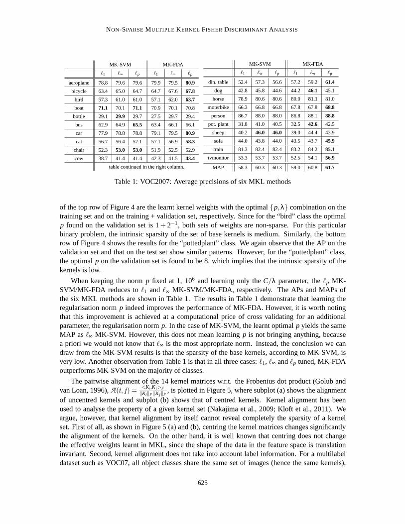
Table 1: VOC2007: Average precisions of six MKL methods

of the top row of Figure 4 are the learnt kernel weights with the optimal{p,λ} combination on thetraining set and on the training + validation set, respectively. Since for the “bird” class the optimalp found on the validation set is 1+ 2−1, both sets of weights are non-sparse. For this particularbinary problem, the intrinsic sparsity of the set of base kernels is medium. Similarly, the bottomrow of Figure 4 shows the results for the “pottedplant” class. We again observe that the AP on thevalidation set and that on the test set show similar patterns. However, for the “pottedplant” class,the optimalp on the validation set is found to be 8, which implies that the intrinsic sparsity of thekernels is low.

When keeping the normp fixed at 1, 106 and learning only theC/λ parameter, theℓp MK-SVM/MK-FDA reduces toℓ1 and ℓ∞ MK-SVM/MK-FDA, respectively. The APs and MAPs ofthe six MKL methods are shown in Table 1. The results in Table 1 demonstrate that learning theregularisation normp indeed improves the performance of MK-FDA. However, it is worth notingthat this improvement is achieved at a computational price of cross validating for an additionalparameter, the regularisation normp. In the case of MK-SVM, the learnt optimalp yields the sameMAP asℓ∞ MK-SVM. However, this does not mean learningp is not bringing anything, becausea priori we would not know thatℓ∞ is the most appropriate norm. Instead, the conclusion we candraw from the MK-SVM results is that the sparsity of the base kernels, according to MK-SVM, isvery low. Another observation from Table 1 is that in all three cases:ℓ1, ℓ∞ andℓp tuned, MK-FDAoutperforms MK-SVM on the majority of classes.

The pairwise alignment of the 14 kernel matrices w.r.t. the Frobenius dot product (Golub andvan Loan, 1996),A(i, j) = <Ki ,K j>F

‖Ki‖F‖K j‖F, is plotted in Figure 5, where subplot (a) shows the alignment

of uncentred kernels and subplot (b) shows that of centred kernels.Kernel alignment has beenused to analyse the property of a given kernel set (Nakajima et al., 2009;Kloft et al., 2011). Weargue, however, that kernel alignment by itself cannot reveal completely the sparsity of a kernelset. First of all, as shown in Figure 5 (a) and (b), centring the kernel matrices changes significantlythe alignment of the kernels. On the other hand, it is well known that centringdoes not changethe effective weights learnt in MKL, since the shape of the data in the feature space is translationinvariant. Second, kernel alignment does not take into account label information. For a multilabeldataset such as VOC07, all object classes share the same set of images (hence the same kernels),

625


(a) (b)

Figure 5: VOC07: Alignment of the 14 kernels. (a) Spherically normalised kernels. (b) Spheri-cally normalised and centred kernels. Note the scale difference between the two plots asindicated by the colorbars.

and the labels are different depending on which object class (i.e., which binary problem) is beingconsidered. It is clear from Table 1 that for bothℓp MK-FDA and ℓp MK-SVM, the sparsity of thekernel set is class dependent. This means kernel alignment, which is classindependent, by itselfcannot be expected to identify the kernel set sparsity for all classes. Instead, we hypothesise thatcorrelation analysis using projected labels (Braun et al., 2008) is probably more appropriate.

Finally, note that due to different parameter sets and different normalisation methods used(spherical normalisation in this paper while unit trace normalisation in Yan et al.,2010), the re-sults on VOC07, Caltech101 and Flower17 reported in this paper are slightly different from thosein Yan et al. (2010). However, the trends in the results remain the same, andall conclusions drawnfrom the results remain unchanged.

3.4 Caltech101

In the following three sections, we compare the proposedℓp MK-FDA with several variants ofℓp

MK-SVM on multiclass problems. We start in this section with the Caltech101 objectrecognitiondataset. Caltech101 is a multiclass object recognition benchmark with 101 object categories. Wefollow the popular practice of using 15 randomly selected images per class for training, up to 50randomly selected images per class for testing, and compute the average accuracy over all classes.This process is repeated 3 times, and we report the mean of the average accuracies on the test setthat is achieved with the optimal parameter (C for MK-SVM and λ for MK-FDA). Validation isomitted, as the training of multiclass MK-SVM Shogun on this dataset can be verytime consuming.

We generate 10 kernels in a similar way as in the VOC2007 experiments. In addition to these“informative” kernels, we also construct 10 RBF kernels from 10 sets of random vectors. To testthe robustness of the MKL methods, we repeat the experiment 6 times. We start with only theinformative kernels, and add two more random kernels in each subsequent run.

626


p= 1 p= 1+2−6 p= 1+2−2

p= 2 p= 4 p= 106

Figure 6: Caltech101: Accuracy comparison of three multiclass MKL methods.

Two multiclass MK-SVM implementations are compared against multiclass MK-FDA, namely,MK-SVM Shogun, and the recently proposed online MK-SVM algorithm OBSCURE (Orabonaet al., 2010). For OBSCURE, the parameters are set to default values, except for the MKL normpand the regularisation parameterC. In our experiments,C andλ are chosen from the same set ofvalues that are logarithmically spaced over 4−5 to 44. We use the same set of 12p values as in theVOC07 experiments. Note however that in OBSCURE, the MKL normp is specified equivalentlythrough the block normr, wherer = 2p/(p+ 1). Moreover, OBSCURE requires thatr > 1, sop= r = 1 in the set ofp values is not used for OBSCURE.

The performance of the three MKL methods with various numbers of randomkernels is il-lustrated in Figure 6, where we show results for sixp values, covering the spectrum from highlysparsity-inducing norm, to uniform weighting. Whenp is large, MK-SVM Shogun does not con-verge within 24 hours, so its performance is not plotted forp = 4 andp = 106. We can see fromFigure 6 that, whenp is small, both MK-SVM OBSCURE and MK-FDA are robust to the addednoise, and MK-FDA has a marginal advantage over OBSCURE (e.g.,∼0.003 whenp= 1+2−6).Whenp is large, as expected, the performance of all three methods in general degrades as the num-ber of random kernels increases. However, MK-FDA does so more gracefully than OBSCURE. Onthe other hand, both MK-FDA and MK-SVM OBSCURE outperform MK-SVMShogun by a largemargin on this multiclass problem.

3.5 Oxford Flower17

Oxford Flower17 is a multiclass dataset consisting of 17 categories of flowers with 80 images percategory. This dataset comes with 3 predefined splits into training (17×40 images), validation (17×20 images) and test (17×20 images) sets. Moreover, Nilsback and Zisserman (2008) precomputed

627


method accuracy and std. dev. parameters tuned on val. set

product 85.5± 1.2 C

averaging 84.9± 1.9 C

MKL (SILP) 85.2± 1.5 C

MKL (Simple) 85.2± 1.5 C

CG-Boost 84.8± 2.2 C

LP-β 85.5± 3.0 Cj , j = 1, · · · ,n andδ ∈ (0,1)

LP-B 85.4± 2.4 Cj , j = 1, · · · ,n andδ ∈ (0,1)

ℓp MK-SVM Shogun 86.0± 2.4 p andC jointly

ℓp MK-SVM OBSCURE 85.6± 0.0 p andC jointly

ℓp MK-FDA 87.2± 1.6 p andλ jointly

Table 2: Flower17: Comparison of ten kernel fusion methods.

7 distance matrices using various features, and the matrices are available online.8 We use thesedistance matrices and follow the same procedure as in Gehler and Nowozin (2009) to compute 7kernels:K j(xi ,xi′) = exp(−D j(xi ,xi′)/η j), whereη j is the mean of the pairwise distances for thej th feature.

Table 2 comparesℓp MK-SVM Shogun,ℓp MK-SVM OBSCURE,ℓp MK-FDA, and 7 kernelcombination techniques discussed in Gehler and Nowozin (2009). Note thatthese methods aredirectly comparable since they share the same kernel matrices and the same splits. Forℓp MK-SVMShogun,ℓp MK-SVM OBSCURE andℓp MK-FDA, the parametersp, C andλ are tuned on thevalidation set from the same sets of values as in the Caltech101 experiments. For the other sevenmethods, the corresponding entries in the table are taken directly from Gehler and Nowozin (2009),where: “product” and “sum” refer to the two simplest kernel combination methods, namely, takingthe element-wise geometric mean and arithmetic mean of the kernels, respectively; “MKL (SILP)”and “MKL (Simple)” are essentiallyℓ1 MK-SVM; while “CG-Boost”, “LP-β” and “LP-B” are threeboosting based kernel combination methods.

We can see from Table 2 that the boosting based methods, although performing well on otherdatasets in Gehler and Nowozin (2009), fail to outperform the baseline methods “product” and“averaging”. On the other hand,ℓp MK-FDA not only shows a considerable improvement overall the methods discussed in Gehler and Nowozin (2009), but also outperforms bothℓp MK-SVMShogun andℓp MK-SVM OBSCURE. Note that the optimal test accuracy over all combinationsofparameters achieved by OBSCURE is comparable to that by MK-FDA. However, the performanceon the validation set and that on the test set do not match as well for OBSCURE as for MK-FDA,9

resulting in the lower test accuracy of OBSCURE. Parameters that need to be tuned on the validationset in these methods are also compared in Table 2.

3.6 Protein Subsellular Localisation

In the previous three sections, we have shown that on both binary and multiclass object recognitionproblems,ℓp MK-FDA tends to outperformℓp MK-SVM by a small margin. In this section, wefurther compareℓp MK-FDA and ℓp MK-SVM on a computational biology problem, namely, theprediction of subcellular localisation of proteins (Zien and Ong, 2007; Ongand Zien, 2008).

8. The distance matrices can be found athttp://www.robots.ox.ac.uk/ ˜ vgg/research/flowers/index.html .9. This is indicated by, for example, a lower Spearman or Kendall rank correlation coefficient.

628


norm p 1 32/31 16/15 8/7 4/3 2 4 8 16 ∞

MK-SVM8.18 8.22 8.20 8.21 8.43 9.47 11.00 11.61 11.91 11.85

plant± 0.47 ± 0.45 ± 0.43 ± 0.42 ± 0.42 ± 0.43 ± 0.47 ± 0.49 ± 0.55 ± 0.60

MK-FDA10.86 11.02 10.96 11.07 10.85 10.69 11.28 11.28 11.04 11.35

± 0.42 ± 0.43 ± 0.46 ± 0.43 ± 0.43 ± 0.37 ± 0.45 ± 0.45 ± 0.43 ± 0.46

MK-SVM8.97 9.01 9.08 9.19 9.24 9.43 9.77 10.05 10.23 10.33

nonpl± 0.26 ± 0.25 ± 0.26 ± 0.27 ± 0.29 ± 0.32 ± 0.32 ± 0.32 ± 0.32 ± 0.31

MK-FDA10.93 10.59 10.91 10.89 10.84 11.00 12.12 12.12 11.81 12.15

± 0.31 ± 0.33 ± 0.31 ± 0.32 ± 0.31 ± 0.33 ± 0.41 ± 0.41 ± 0.38 ± 0.41

MK-SVM9.99 9.91 9.87 10.01 10.13 11.01 12.20 12.73 13.04 13.33

psortNeg± 0.35 ± 0.34 ± 0.34 ± 0.34 ± 0.33 ± 0.32 ± 0.32 ± 0.34 ± 0.33 ± 0.35

MK-FDA9.89 10.07 9.95 9.87 9.75 9.74 11.39 11.25 11.27 11.50

± 0.34 ± 0.36 ± 0.35 ± 0.37 ± 0.39 ± 0.37 ± 0.35 ± 0.34 ± 0.35 ± 0.35

MK-SVM13.07 13.01 13.41 13.17 13.25 14.68 15.55 16.43 17.36 17.63

psortPos± 0.66 ± 0.63 ± 0.67 ± 0.62 ± 0.61 ± 0.67 ± 0.72 ± 0.81 ± 0.83 ± 0.80

MK-FDA12.59 13.16 13.07 13.34 13.45 13.63 16.86 16.37 16.56 16.94

± 0.75 ± 0.80 ± 0.80 ± 0.80 ± 0.74 ± 0.70 ± 0.85 ± 0.89 ± 0.87 ± 0.84

Table 3: Protein Subcellular Localisation: comparingℓp MK-FDA and ℓp MK-SVM w.r.t. pre-diction error and its standard error. Prediction error is measured as 1−average MCC inpercentage.

The protein subcellular localisation problem contains 4 datasets, corresponding to 4 differentsets of organisms: plant (plant), non-plant eukaryotes (nonpl), Gram-positive (psortPos) and Gram-negative bacteria (psortNeg). Each of the 4 datasets can be considered as a multiclass classificationproblem, with the number of classes ranging between 3 and 5. For each dataset, 69 kernels thatcapture diverse aspects of protein sequences are available online.10 We download the kernel matri-ces and follow the experimental setup in Kloft et al. (2011) to enable a direct comparison. Morespecifically, for each dataset, we first multiplicatively normalise the kernel matrices. Then for eachof the 30 predefined splits, we use the first 20% of examples for testing andthe rest for training.

In Kloft et al. (2011), the multiclass problem associated with each dataset isdecomposedinto binary problems using the one-vs-rest strategy. This is not necessary in the case of FDA,since FDA by its natures handles both binary and multiclass problems in a principled fashion.For each dataset, we consider the same set of values for the normp as in Kloft et al. (2011):{1,32/31,16/15,8/7,4/3,2,4,8,∞}. In Kloft et al. (2011), the regularisation constant C for MK-SVM is taken from a set of 9 values:{1/32,1/8,1/2,1,2,4,8,32,128}. In our experiments, theregularisation constantλ for MK-FDA is also taken from a set of 9 values, and the values are loga-rithmically spaced over 10−8 to 100.

Again following Kloft et al. (2011), for eachp/λ combination, we evaluate the performance ofℓp MK-FDA w.r.t. average (over the classes) Matthews correlation coefficient (MCC), and report inTable 3 the average of 1−MCC over 30 splits and its standard error. For ease of comparison, wealso show in Table 3 the performance ofℓp MK-SVM as reported in Kloft et al. (2011).

10. The kernels can be downloaded athttp://www.fml.tuebingen.mpg.de/raetsch/suppl/prots ubloc .

629


Table 3 demonstrates that overall the performance ofℓp MK-FDA lags behind that ofℓp MK-SVM, except onpsortNegand onpsortPos, where it has a small edge. Another observation isthat the optimal normp identified by MK-SVM does not necessarily agree with that by MK-FDA.On psortPosthey are in close agreement and both methods favour sparsity-inducing norms. Onplant, nonplandpsortNeg, on the other hand, the norms picked by MK-FDA are larger than thosepicked by MK-SVM. Note, however, that this observation can be slightly misleading, because onthe latter three datasets, the performance curve ofℓp MK-FDA is quite “flat” in the area of optimalperformance. As a result, the optimal norm estimated may not be stable.

3.7 Training Speed

In this section we provide an empirical analysis of the efficiency of the wrapper-basedℓp MK-FDAand various implementations ofℓp MK-SVM. We usep = 1 (or in some cases 1+2−5, 1+2−6)andp= 2 as examples of sparse/non-sparse MKL respectively,11 and study the scalability of MK-FDA and MK-SVM w.r.t. the number of examples and the number of kernels, onboth binary andmulticlass problems.

3.7.1 BINARY CASE: VOC2007

We first compare on the VOC2007 dataset the training speed of three binary MKL methods: thewrapper based binaryℓp MK-FDA in Section 2.1, the binaryℓp MK-SVM Shogun implementa-tion (Sonnenburg et al., 2006, 2010), and the SMO-MKL in Vishwanathanet al. (2010). In theexperiments, interleaved optimisation and analytical update ofβ are used for MK-SVM Shogun.

We first fix the number of training examples to 1000, and vary the number of kernels from 3 to96. We record the time taken to learn the kernel weights, and average overthe 20 binary problems.Figure 7 (a) shows the training time of the six MKL algorithms as functions of the number ofkernels. Next, we fix the number of kernels to 14, and vary the number of examples from 75 to4800. Similarly, in Figure 7 (b) we plot the average training time as functions ofthe number ofexamples.

Figure 7 (a) demonstrates that for small/medium sized problems, when a sparsity-inducing normis used, SMO-MKL is the most efficient; while whenp = 2, MK-FDA can be significantly fasterthan the competing methods. On the other hand, when training efficiency is measured as a func-tion of the number of examples, there is no clear winner, as indicated in Figure7 (b). However,the trends in Figure 7 (b) suggest that on large scale problems, SMO-MKLis likely to be moreefficient than MK-FDA and MK-SVM Shogun. In both cases, MK-FDA has a comparable or bet-ter efficiency than MK-SVM Shogun, despite the fact that MK-SVM Shogunuses the interleavedalgorithm while MK-FDA employs the somewhat wasteful wrapper-based implementation. Again,this trend is likely to flip over on large scale problems. For such problems, onecan adopt either thesquare loss counterpart of the interleaved algorithm, or the square loss counterpart of the SMO-MKLalgorithm, or the limited memory quasi-Newton method, to improve the efficiency ofℓp MK-FDA,as discussed in Section 2.3.

11. Both SMO-MKL and OBSCURE require thatp > 1. Moreover, SMO-MKL is numerically unstable whenp =1+2−6. As a result, we usep= 1+2−5 andp= 1+2−6 as sparsity-inducing norms for SMO-MKL and OBSCURE,respectively.

630


(a) (b)

Figure 7: Training speed on a binary problem: VOC2007. (a) Training time vs. number of kernels,where number of examples is fixed at 1000. (b) Training time vs. number of examples,where number of kernels is fixed at 14.λ = 1 for MK-FDA, andC = 1 for MK-SVMShogun and MK-SVM OBSCURE.

3.7.2 MULTICLASS CASE: CALTECH101

Next we compare three multiclassℓp MKL algorithms on the Caltech101 dataset, namely, thewrapper-based multiclassℓp MK-FDA in Section 2.2, multiclassℓp MK-SVM Shogun, and MK-SVM OBSCURE. We compare the first two methods following similar protocols as inthe binarycase. In Figure 8 (a) we show the average training time over the 3 splits as functions of the numberof kernels (from 2 to 31) when the number of examples is fixed to 101 (one example per class);while plotted in Figure 8 (b) is the average training time as functions of the numberof examples(from 101 to 1515, that is, from one example per class to 15 examples per class) when the numberof kernels is fixed to 10.

Figure 8 shows that on small/medium sized multiclass problems, MK-FDA is in most casesone or two orders of magnitude faster than MK-SVM Shogun. The only exception is that as thenumber of kernels increases, the efficiency ofℓ1 MK-SVM Shogun degrades more gracefully thanℓ1 MK-FDA, and eventually overtakes. Another observation from both Figure 7 and Figure 8 isthat, ℓ2 MK-FDA tends to be more efficient thanℓ1 MK-FDA, despite the fact that in the outersubproblem, the LP solver employed inℓ1 MK-FDA is slightly faster than the QCLP solver inℓ2

MK-FDA. This is becauseℓ1 MK-FDA usually takes a few tens of iterations to converge, whilethe ℓ2 version typically takes less than 5. This difference in the number of iterationsreverses theefficiency advantage of LP over QCLP.

Due to its online nature, the efficiency of OBSCURE has to be measured differently to allowa fair comparison. The OBSCURE algorithm is a two-stage algorithm, and eachstage involvesan iterative process with a parameterT1/T2 controlling the number of iterations. In general the

631


(a) (b)

Figure 8: Training speed on a multiclass problem: Caltech101. MK-FDA vs. MK-SVM Shogun.(a) Training time vs. number of kernels, where number of examples is fixed at 101. (b)Training time vs. number of examples, where number of kernels is fixed at 10. λ = 1 forMK-FDA, andC= 1 for MK-SVM Shogun.

Figure 9: Training speed on a multiclass problem: Caltech101. MK-FDA vs. MK-SVM OB-SCURE. Top row:p = 1+ 2−6. Bottom row: p = 2. The three columns correspondto the three splits. 10 kernels and 101×15= 1515 training examples.

632


larger the values ofT1 andT2, the longer it takes to train, but the more accurate the learnt model.We setT1 = T2 = T and varyT in a set of 11 values from 20 to 210. This allows us to plot acurve of model accuracy against training time. For MK-FDA, the similar curve can be plotted byvarying the convergence thresholdε in a set of 11 values:{20, · · · ,2−6,10−2, · · · ,10−5}. Note thatthe regularisation parameters (λ for MK-FDA andC for OBSCURE) are set to values that yield thehighest classification accuracy.

The resulting time-accuracy curves for all 3 splits of the dataset are presented in Figure 9,where the top row corresponds to the case ofp= 1+2−6 and the bottom row top= 2, and eachcolumn corresponds to one split. It is evident that MK-FDA typically reaches its optimum fasterthan OBSCURE, especially in the case ofp= 2. Moreover, the optimum achieved by MK-FDA is atleast as accurate as that by OBSCURE, confirming our findings in Section 3.4. All the training timereported in this section is measured on a single core of an Intel Xeon E55202.27GHz processor.

4. Discussion: FDA vs. SVM

The empirical observation that MK-FDA tends to outperform MK-SVM on image categorisationdatasets matches well with our experience with single kernel FDA and single kernel SVM on severalother object/image/video classification benchmarks, including VOC2008, VOC2009, VOC2010,12

Trecvid2008, Trecvid2009,13 and ImageCLEF2010.14 In this section, we discuss the connectionbetween (MK-)SVM and (MK-)FDA from perspectives of both loss function and version space,and attempt to explain their different performance.

It is well known that many machine learning problems essentially boil down to function learn-ing. In the supervised scenario, it is intuitive to learn the function by minimising the empirical lossfor the given set of labelled input/output pairs{xi ,yi}

mi=1, with respect to some loss function. How-

ever, such an empirical risk minimisation principle is ill-posed and therefore does not generalise(Tikhonov and Arsenin, 1977; Vapnik, 1999). Regularisation tries to restore well-posedness of thelearning problem, by restricting the complexity of the function set over which the empirical lossis minimised. By (implicitly) mapping the data into a high dimensional feature space, thiscan beconveniently done in the form of Tikhonov regularisation:

minw

12||w||2+C

m

∑i=1

V( f (φ(xi)),yi), (27)

whereφ(xi) is the mapping to the feature space,f (φ(xi)) = wTφ(xi) is the linear function to belearnt, the complexity of the function set is regularised by1

2||w||2, andV(·, ·) measures the empiricalloss. Learning machines with the form of Equation (27) are collectively termed regularised kernelmachines, a name capturing the two key aspects of them: regularisation, and kernel mapping. Notethat in the formulation above, the unregularised bias termb in standard SVM is absent from thelinear function. As shown in Keerthi and Shevade (2003); Poggio et al.(2004), the two formulations,with and withoutb, can be made equivalent by transforming the kernel function.

The setting in Equation (27) is very general, in the sense that many state-of-the-art machinelearning techniques can be realised by plugging in different loss functions. For example, the hingelossV( f (φ(x)),y) = (1− y f(φ(x)))+, where(·)+ = max(·,0), gives rise to the well known SVM,

12. More information on VOC can be found athttp://pascallin.ecs.soton.ac.uk/challenges/VOC .13. More information on Trecvid can be found athttp://www-nlpir.nist.gov/projects/trecvid .14. More information on ImageCLEF can be found athttp://www.imageclef.org/2010 .

633


probably the most popular learning machine in the past ten years. On the other hand, along with thesuccess of SVM, regularised kernel machines using the square lossV( f (φ(x)),y) = (y− f (φ(x)))2

have emerged several times under various names, including: regularisednetworks (RN) (Girosiet al., 1995; Evgeniou et al., 2000), regularised least squares (RLS)(Rifkin, 2002), kernel ridgeregression (KRR) (Saunders et al., 1998; Hastie et al., 2002), least squares support vector machines(LSSVM) (Suykens and Vandewalle, 1999; Gestel et al., 2002), proximal support vector machines(PSVM) (Fung and Mangasarian, 2001). In particular, shortly after the proposal of kernel FDA(Mika et al., 1999; Baudat and Anouar, 2000), its regularised versionwas shown to be yet anotherequivalent formulation (Duda et al., 2000; Rifkin, 2002; Gestel et al., 2002).

There is a long list of literature which compares the performance of FDA andSVM, for example,Mika (2002), Rifkin (2002), Cai et al. (2007) and Ye et al. (2008), with most of them reporting bothmethods yield virtually identical performance, and the rest claiming there is a small advantagetowards one method or the other. It is speculated in Mika et al. (1999) that the superior performanceof FDA over SVM in their experiments is due to the fact that FDA uses all training examples in thetest stage while SVM uses only the support vectors. However, a more elegant way of explaining thedifferent performance of SVM and FDA is probably from the perspective of version space. Versionspace is the space of all consistent hypotheses, that is, allw’s that correspond to hyperplanes withzero training error (Rujan, 1997). Note that with a full rank kernel matrix, linear separability inthe feature space and therefore the existence of version space is guaranteed. It is shown in Rujan(1997) that the optimal hyperplane in the Bayes sense, which requires theknowledge of the jointdistribution onX ×Y thus not obtainable in practice, is arbitrarily close (with increasing trainingsample size) to the centre of mass of the version space.

Algorithms that explicitly approximate the Bayes point were later termed Bayes point machine(BPM) in Herbrich et al. (2001). Herbrich et al. (2001) also prove that the hyperplane found bySVM corresponds to the centre of the largest inscribed ball of the version space. In this light, SVMcan be viewed as an approximation to BPM. This approximation is reasonable if the version spaceis regularly shaped, but can be weak otherwise (Rujan, 1997; Herbrich et al., 2001; Mika, 2002).For example, experiments in Herbrich et al. (2001) show that BPM consistently outperforms SVM.Recently, an ellipsoid SVM was proposed (Momma et al., 2010), where the idea is to improve theapproximation to the Bayes point by using the centre of the largest inscribedellipsoid, instead ofthat of the ball. We conjecture that for certain kernels (e.g., kernels generated using local descriptorsand bag-of-words model, as those used in image categorisation problems),due to the different lossfunctions used, the hyperplane given by FDA is closer to the Bayes pointthan that given by SVM,resulting in the superior performance of (MK-)FDA in our experiments. How to decide without avalidation process whether (MK-)FDA or (MK-SVM) is more suitable for a given kernel (set), andhow to incorporate explicit BPM approximation into MKL, are interesting research directions forthe future.

5. Conclusions

In this paper we have incorporated latest advances in both non-sparseMKL formulation and MKLoptimisation techniques into MK-FDA. We have presented a non-sparse version of MK-FDA basedon anℓp norm regularisation of kernel weights, and have discussed several of its reformulations andassociated optimisation strategies, including wrapper and interleaved algorithms for its saddle pointformulation, and an SMO-based scheme for its dual formulation.

634


We carried out extensive evaluation on six datasets from various application areas. Our resultsindicate that the optimal normp, and therefore the “intrinsic sparsity” of the base kernels, can beestimated on an independent validation set. This estimation can be exploited in manypracticalapplications where there is no prior knowledge on how informative the channels are. We have alsocompared closely the performance ofℓp MK-FDA and that of several variants ofℓp MK-SVM.On object and image categorisation problems, MK-FDA tends to have a small advantage. Thisobservation is consistent with our findings elsewhere regarding the performance of single kernelFDA/SVM. In terms of training time, the wrapper-based MK-FDA implementation has similar orfavourable efficiency on small to medium sized problems when compared against state-of-the-artMKL techniques. On large scale problems, alternative optimisation strategies discussed in the papershould be employed to improve the efficiency and scalability of MK-FDA.

Finally, we have provided a discussion on the connection between (MK-)FDA and (MK-)SVMfrom the perspectives of both loss function and version space, underthe unified framework of regu-larised kernel machines.

Acknowledgments

We would like to thank Soren Sonnenburg, Gunnar Ratsch, Alexander Binder for their help on theShogun toolbox, Jianhui Chen and Jieping Ye for help on their discriminantMKL package, andMarius Kloft for helpful discussions. We would also like to thank the anonymous reviewers and theeditors for their valuable comments and suggestions. The work presented inthis paper is supportedby the EPSRC/UK grant EP/F069626/1 ACASVA Project.

Appendix A. Multiclass ℓp MK-FDA Saddle Point Formulation

In this appendix, we first derive the saddle point formulation of multiclass MKL for a generalconvex loss. Multiclass MK-FDA saddle point problem is then derived as aspecial case of it. Usingthe output encoding scheme in Equation (18), multiclass MKL for a general convex loss functionV(ξik,hik) can be stated as:

minw jk,ξik,β

c

∑k=1

(

12

n

∑j=1

||w jk||2

β j+C

m

∑i=1

V(ξik,hik)

)

(28)

s.t.n

∑j=1

wTjkφ j(xi) = ξik, ∀i, ∀k; β ≥ 0; ||β||2p ≤ 1.

We build the Lagrangian of Equation (28):

L =c

∑k=1

(

12

n

∑j=1

||w jk||2

β j+C

m

∑i=1

V(ξik,hik)

)

+ζ(12||β||2p−

12)

−c

∑k=1

m

∑i=1

αik

( n

∑j=1

wTjkφ j(xi)−ξik

)

,

635


set to zero the derivatives of the Lagrangian w.r.t.w jk, and substitute back. After some rearrange-ments we have:

L =c

∑k=1

(

Cm

∑i=1

V(ξik,hik)+m

∑i=1

αikξik −12

n

∑j=1

αTk β jK jαk

)

+ζ(12||β||2p−

12),

whereαk = (α1k, · · · ,αmk)T . Following Theorem 1 of Kloft et al. (2011) it can be shown that at

the optimum||β||2p = 1. Using this fact we arrive at the multiclass MKL saddle point problem for ageneral loss function:

minξik,β

maxαik

c

∑k=1

(

Cm

∑i=1

V(ξik,hik)+m

∑i=1

αikξik −12

n

∑j=1

αTk β jK jαk

)

(29)

s.t. β ≥ 0; ||β||2p ≤ 1.

At this point any convex loss function can be plugged into Equation (29). Take the square lossV(ξik,hik) =

12(ξik − hik)

2 as an example. Setting to zero the derivatives ofL w.r.t. ξik we haveξik = hik−αik/C. Plugging this into Equation (29) and rearranging we arrive at the multiclassMKLsaddle point problem for square loss, that is, multiclass multiple kernel regularised least squares(MK-RLS):

minβ

maxαk

c

∑k=1

(

hTk αk−

12C

αTk αk−

12

n

∑j=1

αTk β jK jαk

)

(30)

s.t. β ≥ 0; ||β||2p ≤ 1,

where thec classes are coupled through the common set of kernel weightsβ. By making substitu-tionsαk →

C2αk and thenC→ 1

λ , it directly follows that the MK-RLS in Equation (30) is equivalentto the MK-FDA in Equation(19).

Appendix B. Multiclass ℓp MK-FDA Dual Formulation

In this appendix, we derive the dual formulation of multiclass MK-FDA. We again consider mul-ticlass MKL with a general convex loss, but following Vishwanathan et al. (2010) this time weimpose the norm constraint in the form of Tikhonov regularisation instead ofIvanov regularisation:

minw jk,ξik,β

c

∑k=1

(

12

n

∑j=1

‖w jk‖2

β j+C

m

∑i=1

V(ξik,hik)

)

+µ2‖β‖2

p (31)

s.t.n

∑j=1

wTjkφ j(xi) = ξik, ∀i, ∀k; β ≥ 0.

Note however that the switching from Ivanov to Tikhonov regularisation is not essential for thederivation in the following. The dual program for Ivanov regularisationin Equation (28) can bederived in a similar way.

Building the Lagrangian of Equation (31):

L =c

∑k=1

(

12

n

∑j=1

‖w jk‖2

β j+C

m

∑i=1

V(ξik,hik)

)

+µ2‖β‖2

p−n

∑j=1

γ jβ j

−c

∑k=1

m

∑i=1

αik

( n

∑j=1

wTjkφ j(xi)−ξik

)

,

636


and setting to zero the derivatives w.r.t.β j , we have:

µ(n

∑j=1

βpj )

2p−1βp−1

j = γ j +12

c

∑k=1

αTk K jαk. (32)

Multiplying both sides of Equation (32) byβ j and then taking summation overj gives us:

µ‖β‖2p =

n

∑j=1

β j(γ j +12

c

∑k=1

αTk K jαk),

or equivalently:n

∑j=1

γ jβ j =−12

n

∑j=1

c

∑k=1

αTk β jK jαk+µ‖β‖2

p. (33)

On the other hand, raise both sides of Equation (32) to powerpp−1 and then take summation over

j, we have:

µ‖β‖2p =

1µ

∥

∥

∥

∥

(

γ j +12

c

∑k=1

αTk K jαk

)n

j=1

∥

∥

∥

∥

2

q, (34)

whereq= pp−1 is the dual norm ofp.

Now let us set the derivatives ofL w.r.t. w jk also to zero, and substitute the result and Equa-tion (33), Equation (34) back intoL . Using the fact thatγ j = 0 at the optimum (Vishwanathan et al.,2010), and after some rearrangements we arrive at:

L =c

∑k=1

(

Cm

∑i=1

V(ξik,hik)+m

∑i=1

αikξik

)

−18µ

∥

∥

∥

∥

( c

∑k=1

αTk K jαk

)n

j=1

∥

∥

∥

∥

2

q. (35)

At this point any convex loss function can be plugged into Equation (35) to recover the correspond-ing multiclass MKL dual. We again take the square lossV(ξik,hik) =

12(ξik −hik)

2 as an example.Setting to zero the derivatives ofL w.r.t. ξik we haveξik = hik −αik/C. Plugging this into Equa-tion (35) and rearranging we arrive at the multiclass MK-RLS dual problem:

maxαk

c

∑k=1

(

hTk αk−

12C

αTk αk

)

−18µ

∥

∥

∥

∥

( c

∑k=1

αTk K jαk

)n

j=1

∥

∥

∥

∥

2

q. (36)

Unlike the saddle point formulation in Equation (30), the kernel weightsβ have been eliminatedfrom Equation (36). Despite this, Equation (30) and Equation (36) are equivalent, in the sense thatfor any givenC there exist aµ (and vice versa) such that the optimal solutions to both problems areidentical (Kloft et al., 2011).

Finally, substituting Equation (34) andγ j = 0 into Equation (32), we show that once the optimalαk are found by solving Equation (36), the kernel weightsβ are given by:

β j =12µ

( n

∑j=1

(c

∑k=1

αTk K jαk)

q)

1q−

1p

(c

∑k=1

αTk K jαk)

qp .

637


References

F. Bach and G. Lanckriet. Multiple kernel learning, conic duality, and the smo algorithm. InInternational Conference on Machine Learning, 2004.

G. Baudat and F. Anouar. Generalized discriminant analysis using a kernel approach. NeuralComputation, 12:2385–2404, 2000.

O. Bousquet and D. Herrmann. On the complexity of learning the kernel matrix. In Advances inNeural Information Processing Systems, 2003.

M. Braun, J. Buhmann, and K. Muller. On relevant dimensions in kernel feature spaces.Journal ofMachine Learning Research, 9:1875–1908, 2008.

D. Cai, X. He, and J. Han. Efficient kernel discriminant analysis via spectral regression. InInter-national Conference on Data Mining, 2007.

H. Cai, K. Mikolajczyk, and J. Matas. Learning linear discriminant projections for dimensionalityreduction of image descriptors.IEEE Transactions on Pattern Analysis and Machine Intelligence,33(2):338–352, 2011.

O. Chapelle, V. Vapnik, O. Bousquet, and S. Mukherjee. Choosing multipleparameters for supportvector machines.Machine Learning, 46:131–159, 2002.

C. Cortes, M . Mohri, and A. Rostamizadeh. L2 regularization for learningkernels. InUncertaintyin Artificial Intelligence, 2009.

N. Cristianini, J. Shawe-Taylor, A. Elisseeff, and J. Kandola. On kernel-target alignment. InAd-vances in Neural Information Processing Systems, 2002.

G. Csurka, C. Dance, L. Fan, J. Willamowski, and C Bray. Visual categorization with bags ofkeypoints. InECCV workshop on Statistical Learning in Computer Vision, 2004.

R. Duda, P. Hart, and D. Stork.Pattern Classification. Wiley, 2000.

M. Everingham, L. van Gool, C. Williams, J. Winn, and A. Zisserman. The PAS-CAL Visual Object Classes Challenge 2007 (VOC2007) Results. http://www.pascal-network.org/challenges/VOC/voc2007/workshop/index.html, 2007.

M. Everingham, L. van Gool, C. Williams, J. Winn, and A. Zisserman. The PAS-CAL Visual Object Classes Challenge 2008 (VOC2008) Results. http://www.pascal-network.org/challenges/VOC/voc2008/workshop/index.html, 2008.

T. Evgeniou, M. Pontil, and T. Poggio. Regularization networks and support vector machines.Advances in Computational Mathematics, 13:1–50, 2000.

L. Fei-Fei, R. Fergus, and P. Perona. One-shot learning of object categories.IEEE Transactions onPattern Analysis and Machine Intelligence, 28(4):594–611, 2006.

R. Fisher. The use of multiple measurements in taxonomic problems.Annals of Eugenics, 7:179–188, 1936.

638


G. Fung and O. L. Mangasarian. Proximal support vector machine classifier. In InternationalConference on Knowledge Discovery and Data Mining, 2001.

P. Gehler and S. Nowozin. On feature combination for multiclass object classification. In Interna-tional Conference on Computer Vision, 2009.

J. Gemert, J. Geusebroek, C. Veenman, and A. Smeulders. Kernel codebooks for scene categoriza-tion. In European Conference on Computer Vision, 2008.

T. Gestel, J. Suykens, G. Lanckriet, A. Lambrechts, B. Moor, and J. Vandewalle. Bayesian frame-work for least-squares support vector machine classifiers, gaussianprocesses, and kernel fisherdiscriminant analysis.Machine Learning, 14(5):1115–1147, 2002.

F. Girosi, M. Jones, and T. Poggio. Regularization theory and neural networks architectures.NeuralComputation, 7:219–269, 1995.

G. Golub and C. van Loan.Matrix Computations. John Hopkins University Press, third edition,1996.

K. Grauman and T. Darrell. The pyramid match kernel: Efficient learning withsets of features.Journal of Machine Learning Research, 8:725–760, 2007.

T. Hastie, R. Tibshirani, and J. Friedman.The Elements of Statistical Learning. Springer, secondedition, 2002.

R. Herbrich, T. Graeple, and C. Campbell. Bayes point machines.Journal of Machine LearningResearch, 1:245–279, 2001.

R. Hettich and K. Kortanek. Semi-infinite programming: Theory, methods, andapplications.SIAMReview, 35(3):380–429, 1993.

T. Joachims.Making Large-Scale Support Vector Machine Learning Practical. MIT Press, Cam-bridge, MA, 1988.

S. Keerthi and S. Shevade. Smo algorithm for least squares svm formulations.Neural Computation,15(2):487–507, 2003.

S. Kim, A. Magnani, and S. Boyd. Optimal kernel selection in kernel fisherdiscriminant analysis.In International Conference on Machine Learning, 2006.

M. Kloft, U. Brefeld, P. Laskov, and S. Sonnenburg. Non-sparse multiple kernel learning. InNIPSWorkshop on Kernel Learning: Automatic Selection of Optimal Kernels, 2008.

M. Kloft, U. Brefeld, S. Sonnenburg, and A. Zien. Efficient and accurate lp-norm mkl. InAdvancesin Neural Information Processing Systems, 2009.

M. Kloft, U. Brefeld, S. Sonnenburg, and A. Zien. Lp norm multiple kernel learning. Journal ofMachine Learning Research, 12:953–997, 2011.

G. Lanckriet, N. Cristianini, P. Bartlett, L. E. Ghaoui, and M. Jordan. Learning teh kernel matrixwith semi-definite programming. InInternational Conference on Machine Learning, 2002.

639


G. Lanckriet, N. Cristianini, P. Bartlett, L. E. Ghaoui, and M. Jordan. Learning the kernel matrixwith semidefinite programming.Journal of Machine Learning Research, 5:27–72, 2004.

S. Lazebnik, C. Schmid, and J. Ponce. Beyond bags of features: Spatial pyramid matching for rec-ognizing natural scene categories. InInternational Conference on Computer Vision and PatternRecognition, 2006.

D. Liu and J. Nocedal. On the limited memory method for large scale optimization.MathematicalProgramming B, 45(3):503–528, 1989.

J. Lopez and J. Suykens. First and second order smo algorithms for ls-svm classifiers.NeuralProcessing Letters, 33(1):31–44, 2011.

D. Lowe. Distincetive image features from scale-invariant keypoints.International Journal ofComputer Vision, 60(2):91–110, 2004.

S. Mika. Kernel fisher discriminants. PhD Thesis, University of Technology, Berlin, Germany,2002.

S. Mika, G. Ratsch, J. Weston, B. Scholkopf, and K. Muller. Fisher discriminant analysis withkernels. InIEEE Signal Processing Society Workshop: Neural Networks for Signal Processing,1999.

K. Mikolajczyk and C. Schmid. A performance evaluation of local descriptors. IEEE Transactionson Pattern Analysis and Machine Intelligence, 27(10):1615–1630, 2005.

M. Momma, K. Hatano, and H. Nakayama. Ellipsoidal support vector machines. InAsian Confer-ence on Machine Learning, 2010.

S. Nakajima, A. Binder, C. Muller, W. Wojcikiewicz, M. Kloft, U. Brefeld, K.Muller, andM. Kawanabe. Multiple kernel learning for object classification. Technical Report onInformation-Based Induction Sciences, 2009.

M. Nilsback and A. Zisserman. Automated flower classification over a large number of classes. InIndian Conference on Computer Vision, Graphics and Image Processing, 2008.

C. Ong and A. Zien. An automated combination of kernels for predicting protein subcellular local-ization. InWorkshop on Algorithms in Bioinformatics, 2008.

C. Ong, A. Smola, and R. C. Williamson. Hyperkernels. InAdvances in Neural Information Pro-cessing Systems, 2003.

F. Orabona and L. Jie. Ultra-fast optimization algorithm for sparse multi kernel learning. InInter-national Conference on Machine Learning, 2011.

F. Orabona, L. Jie, and B. Caputo. Online-batch strongly convex multi kerenl learning. InInterna-tional Conference on Computer Vision and Pattern Recognition, 2010.

T. Poggio, S. Mukherjee, R. Rifkin, A. Rakhlin, and A. Verri. B. InConference on Uncertainty inGeometric Computations, 2004.

640


A. Rakotomamonjy, F. Bach, Y. Grandvalet, and S. Canu. Simplemkl.Journal of Machine LearningResearch, 9:2491–2521, 2008.

G. Ratsch. Robust boosting via convex optimization. PhD Thesis, University ofPotsdam, Potsdam,Germany, 2001.

R. Rifkin. Everything old is new again: a fresh look at historical approaches in machine learning.PhD Thesis, Massachusetts Institute of Technology, Boston, USA, 2002.

P. Rujan. Playing billiard in version space.Neural Computation, 9:99–122, 1997.

K. Sande, T. Gevers, and C. Snoek. Evaluation of color descriptors for object and scene recognition.In International Conference on Computer Vision and Pattern Recognition, 2008.

C. Saunders, A. Gammerman, and V. Vovk. Ridge regression learning algorithm in dual variables.In International Conference on Machine Learning, 1998.

B. Scholkopf and A. Smola.Learning with Kernels. MIT Press, 2002.

B. Scholkopf, A. Smola, and K. Muller. Kernel principal component analysis.Advances in KernelMethods: Support Vector Learning, pages 327–352, 1999.

J. Shawe-Taylor and N. Cristianini.Kernel Methods for Pattern Analysis. Cambridge UniversityPress, 2004.

C. Snoek, M. Worring, J. Gemert, J. Geusebroek, and A. Smeulders. The challenge problem forautomated detection of 101 semantic concepts in multimedia. InACM Multimedia Conference,2006.

S. Sonnenburg, G. Ratsch, C. Schafer, and B. Scholkopf. Large scale multiple kernel learning.Journal of Machine Learning Research, 7:1531–1565, 2006.

S. Sonnenburg, G. Ratsch, S. Henschel, C. Widmer, J. Behr, A. Zien adn F. Bona, A. Binder, C. Gehl,and V. Franc. The shogun machine learning toolbox.Journal of Machine Learning Research, 11:1799–1802, 2010.

J. Suykens and J. Vandewalle. Least squares support vector machine classifiers.Neural ProcessingLetters, 9:293–300, 1999.

M. Szafranski, Y. Grandvalet, and A. Rakotomamonjy. Composite kernel learning. InInternationalConference on Machine Learning, 2008.

A. Tahir, J. Kittler, K. Mikolajczyk, F. Yan, K. Sande, and T. Gevers. Visual category recognition us-ing spectral regression and kernel discriminant analysis. InInternational Workshop on SubspaceMethods, 2009.

A. Tikhonov and V. Arsenin.Solutions of Ill-Posed Problems. Winston, Washington DC, 1977.

V. Vapnik. The Nature of Statistical Learning Theory. Springer-Verlag, 1999.

S. Vishwanathan, Z. Sun, and N. Theera-Ampornpunt. Multiple kernel learning and the smo algo-rithm. In Advances in Neural Information Processing Systems, 2010.

641


F. Yan, J. Kittler, K. Mikolajczyk, and A. Tahir. Non-sparse multiple kernel learning for fisherdiscriminant analysis. InInternational Conference on Data Mining, 2009a.

F. Yan, K. Mikolajczyk, J. Kittler, and A. Tahir. A comparison of l1 norm and l2 norm multiplekernel svms in image and video classification. InInternational Workshop on Content-BasedMultimedia Indexing, 2009b.

F. Yan, K. Mikolajczyk, M. Barnard, H. Cai, and J. Kittler. Lp norm multiple kernel fisher dis-criminant analysis for object and image categorisation. InInternational Conference on ComputerVision and Pattern Recognition, 2010.

J. Ye, S. Ji, and J. Chen. Multi-class discriminant kernel learning via convex programming.Journalof Machine Learning Research, 9:719–758, 2008.

J. Zhang, M. Marszalek, S. Lazebnik, and C. Schmid. Local featuresand kernels for classification oftexture and object categories: A comprehensive study.International Journal of Computer Vision,73(2):213–238, 2007.

A. Zien and C. Ong. Multiclass multiple kernel learning. InInternational Conference on MachineLearning, 2007.

642

non-sparse multiple kernel fisher discriminant analysis

Documents