› ~fbach › inria_summer_school_2011... · kernel methods & sparse methods for computer...
TRANSCRIPT

Kernel methods & sparse methods
for computer vision
Francis Bach
Sierra project, INRIA - Ecole Normale Superieure
CVML Summer School, Paris, July 2011
1

Machine learning
• Supervised learning
– Predict y ∈ Y from x ∈ X , given observations (xi, yi), i = 1, . . . , n
• Unsupervised learning
– Find structure in x ∈ X , given observations xi, i = 1, . . . , n
• Application to many problems and data types:
– Computer vision
– Bioinformatics
– Text processing
– etc.
• Specifity: exchanges between theory / algorithms / applications
2

Machine learning for computer vision
• Multiplication of digital media
• Many different tasks to be solved
– Associated with different machine learning problems
– Massive data to learn from
3

Image retrieval
⇒ Classification, ranking, outlier detection
4

Image retrieval
Classification, ranking, outlier detection
5

Image retrieval
Classification, ranking, outlier detection
6

Image annotation
Classification, clustering
7

Object recognition ⇒ Multi-label classification
8

Personal photos
⇒ Classification, clustering, visualization
9

Machine learning for computer vision
• Multiplication of digital media
• Many different tasks to be solved
– Associated with different machine learning problems
– Massive data to learn from
• Similar situations in many fields (e.g., bioinformatics)
10

Machine learning for bioinformatics (e.g., proteins)
1. Many learning tasks on proteins
• Classification into functional or structural classes
• Prediction of cellular localization and interactions
2. Massive data
11

Machine learning for computer vision
• Multiplication of digital media
• Many different tasks to be solved
– Associated with different machine learning problems
– Massive data to learn from
• Similar situations in many fields (e.g., bioinformatics)
⇒ Machine learning for high-dimensional data
12

Supervised learning and regularization
• Data: xi ∈ X , yi ∈ Y, i = 1, . . . , n
• Minimize with respect to function f ∈ F :n∑
i=1
ℓ(yi, f(xi)) +λ
2‖f‖2
Error on data + Regularization
Loss & function space ? Norm ?
• Two theoretical/algorithmic issues:
– Loss
– Function space / norm
13

Course outline
1. Losses for particular machine learning tasks
• Classification, regression, etc...
2. Regularization by Hilbertian norms (kernel methods)
• Kernels and representer theorem
• Convex duality, optimization and algorithms
• Kernel methods
• Kernel design
3. Regularization by sparsity-inducing norms
• ℓ1-norm regularization
• Multiple kernel learning
• Theoretical results
• Learning on matrices
14

Losses for regression (Shawe-Taylor and Cristianini, 2004)
• Response: y ∈ R, prediction y = f(x),
– quadratic (square) loss ℓ(y, f(x)) = 12(y − f(x))2
– Not many reasons to go beyond square loss!
−3 −2 −1 0 1 2 30
1
2
3
4
y−f(x)
square
15

Losses for regression (Shawe-Taylor and Cristianini, 2004)
• Response: y ∈ R, prediction y = f(x),
– quadratic (square) loss ℓ(y, f(x)) = 12(y − f(x))2
– Not many reasons to go beyond square loss!
• Other convex losses “with added benefits”
– ε-insensitive loss ℓ(y, f(x)) = (|y − f(x)| − ε)+– Huber loss (mixed quadratic/linear): robustness to outliers
−3 −2 −1 0 1 2 30
1
2
3
4
y−f(x)
squareε−insensitiveHuber
16

Losses for classification (Shawe-Taylor and Cristianini, 2004)
• Label : y ∈ −1, 1, prediction y = sign(f(x))
– loss of the form ℓ(y, f(x)) = ℓ(yf(x))
– “True” cost: ℓ(yf(x)) = 1yf(x)<0
– Usual convex costs:
−3 −2 −1 0 1 2 3 40
1
2
3
4
5
0−1hingesquarelogistic
• Differences between hinge and logistic loss: differentiability/sparsity
17

Image annotation ⇒ multi-class classification
18

Losses for multi-label classification (Scholkopf and
Smola, 2001; Shawe-Taylor and Cristianini, 2004)
• Two main strategies for k classes (with unclear winners)
1. Using existing binary classifiers (efficient code!) + voting schemes
– “one-vs-rest” : learn k classifiers on the entire data
– “one-vs-one” : learn k(k−1)/2 classifiers on portions of the data
19

Losses for multi-label classification - Linear predictors
• Using binary classifiers (left: “one-vs-rest”, right: “one-vs-one”)
3
2
1
3
2
1
20

Losses for multi-label classification (Scholkopf and
Smola, 2001; Shawe-Taylor and Cristianini, 2004)
• Two main strategies for k classes (with unclear winners)
1. Using existing binary classifiers (efficient code!) + voting schemes
– “one-vs-rest” : learn k classifiers on the entire data
– “one-vs-one” : learn k(k−1)/2 classifiers on portions of the data
2. Dedicated loss functions for prediction using argmaxi∈1,...,k fi(x)
– Softmax regression: loss = − log(efy(x)/∑k
i=1 efi(x))
– Multi-class SVM - 1: loss =∑k
i=1(1 + fi(x)− fy(x))+– Multi-class SVM - 2: loss = maxi∈1,...,k(1 + fi(x)− fy(x))+
• Strategies do not consider same predicting functions
21

Losses for multi-label classification - Linear predictors
• Using binary classifiers (left: “one-vs-rest”, right: “one-vs-one”)
3
2
1
3
2
1
• Dedicated loss function
3
2
1
22

Image retrieval ⇒ ranking
23

Image retrieval ⇒ outlier/novelty detection
24

Losses for ther tasks
• Outlier detection (Scholkopf et al., 2001; Vert and Vert, 2006)
– one-class SVM: learn only with positive examples
• Ranking
– simple trick: transform into learning on pairs (Herbrich et al.,
2000), i.e., predict x > y or x 6 y– More general “structured output methods” (Joachims, 2002)
• General structured outputs
– Very active topic in machine learning and computer vision
– see, e.g., Taskar (2005)
25

Dealing with asymmetric cost or unbalanced data in
binary classification
• Two cases with similar issues:
– Asymmetric cost (e.g., spam filterting, detection)
– Unbalanced data, e.g., lots of positive examples (example:
detection)
• One number is not enough to characterize the asymmetric
properties
– ROC curves (Flach, 2003) – cf. precision-recall curves
• Training using asymmetric losses (Bach et al., 2006)
minf∈F
C+
∑
i,yi=1
ℓ(yif(xi)) + C−∑
i,yi=−1
ℓ(yif(xi)) + ‖f‖2
26

ROC curves
• ROC plane (u, v)
• u = proportion of false positives = P (f(x) = 1|y = −1)
• v = proportion of true positives = P (f(x) = 1|y = 1)
• Plot a set of classifiers fγ(x) for γ ∈ R
v
1false positives0
true
pos
itive
s1
u
27

Course outline
1. Losses for particular machine learning tasks
• Classification, regression, etc...
2. Regularization by Hilbertian norms (kernel methods)
• Kernels and representer theorem
• Convex duality, optimization and algorithms
• Kernel methods
• Kernel design
3. Regularization by sparsity-inducing norms
• ℓ1-norm regularization
• Multiple kernel learning
• Theoretical results
• Learning on matrices
28

Regularizations
• Main goal: avoid overfitting (see, e.g. Hastie et al., 2001)
• Two main lines of work:
1. Use Hilbertian (RKHS) norms
– Non parametric supervised learning and kernel methods
– Well developped theory (Scholkopf and Smola, 2001; Shawe-
Taylor and Cristianini, 2004; Wahba, 1990)
2. Use “sparsity inducing” norms
– main example: ℓ1-norm ‖w‖1 =∑p
i=1 |wi|– Perform model selection as well as regularization
– Theory “in the making”
• Goal of (this part of) the course: Understand how and when
to use these different norms
29

Kernel methods for machine learning
• Definition: given a set of objects X , a positive definite kernel is
a symmetric function k(x, x′) such that for all finite sequences of
points xi ∈ X and αi ∈ R,
∑
i,j αiαjk(xi, xj) > 0
(i.e., the matrix (k(xi, xj)) is symmetric positive semi-definite)
• Main example: k(x, x′) = 〈Φ(x),Φ(x′)〉
30

Kernel methods for machine learning
• Definition: given a set of objects X , a positive definite kernel is
a symmetric function k(x, x′) such that for all finite sequences of
points xi ∈ X and αi ∈ R,
∑
i,j αiαjk(xi, xj) > 0
(i.e., the matrix (k(xi, xj)) is symmetric positive semi-definite)
• Aronszajn theorem (Aronszajn, 1950): k is a positive definite
kernel if and only if there exists a Hilbert space F and a mapping
Φ : X 7→ F such that
∀(x, x′) ∈ X 2, k(x, x′) = 〈Φ(x),Φ(x′)〉H• X = “input space”, F = “feature space”, Φ = “feature map”
• Functional view: reproducing kernel Hilbert spaces
31

Classical kernels: kernels on vectors x ∈ Rd
• Linear kernel k(x, y) = x⊤y
– Φ(x) = x
• Polynomial kernel k(x, y) = (1 + x⊤y)d
– Φ(x) = monomials
• Gaussian kernel k(x, y) = exp(−α‖x− y‖2)– Φ(x) =??
• PROOF
32

Reproducing kernel Hilbert spaces
• Assume k is a positive definite kernel on X × X
• Aronszajn theorem (1950): there exists a Hilbert space F and a
mapping Φ : X 7→ F such that
∀(x, x′) ∈ X 2, k(x, x′) = 〈Φ(x),Φ(x′)〉H• X = “input space”, F = “feature space”, Φ = “feature map”
• RKHS: particular instantiation of F as a function space
– Φ(x) = k(·, x)– function evaluation f(x) = 〈f,Φ(x)〉– reproducing property: k(x, y) = 〈k(·, x), k(·, y)〉
• Notations : f(x) = 〈f,Φ(x)〉 = f⊤Φ(x), ‖f‖2 = 〈f, f〉
33
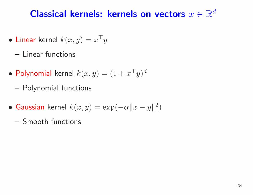
Classical kernels: kernels on vectors x ∈ Rd
• Linear kernel k(x, y) = x⊤y
– Linear functions
• Polynomial kernel k(x, y) = (1 + x⊤y)d
– Polynomial functions
• Gaussian kernel k(x, y) = exp(−α‖x− y‖2)– Smooth functions
34

Classical kernels: kernels on vectors x ∈ Rd
• Linear kernel k(x, y) = x⊤y
– Linear functions
• Polynomial kernel k(x, y) = (1 + x⊤y)d
– Polynomial functions
• Gaussian kernel k(x, y) = exp(−α‖x− y‖2)– Smooth functions
• Parameter selection? Structured domain?
35

Regularization and representer theorem
• Data: xi ∈ X , yi ∈ Y, i = 1, . . . , n, kernel k (with RKHS F)
• Minimize with respect to f : minf∈F
∑ni=1 ℓ(yi, f
⊤Φ(xi)) +λ2‖f‖2
• No assumptions on cost ℓ or n
• Representer theorem (Kimeldorf and Wahba, 1971): optimum is
reached for weights of the form
f =∑n
j=1αjΦ(xj) =∑n
j=1αjk(·, xj)
• PROOF
36

Regularization and representer theorem
• Data: xi ∈ X , yi ∈ Y, i = 1, . . . , n, kernel k (with RKHS F)
• Minimize with respect to f : minf∈F
∑ni=1 ℓ(yi, f
⊤Φ(xi)) +λ2‖f‖2
• No assumptions on cost ℓ or n
• Representer theorem (Kimeldorf and Wahba, 1971): optimum is
reached for weights of the form
f =∑n
j=1αjΦ(xj) =∑n
j=1αjk(·, xj)
• α ∈ Rn dual parameters, K ∈ R
n×n kernel matrix:
Kij = Φ(xi)⊤Φ(xj) = k(xi, xj)
• Equivalent problem: minα∈Rn∑n
i=1 ℓ(yi, (Kα)i) +λ2α
⊤Kα
37
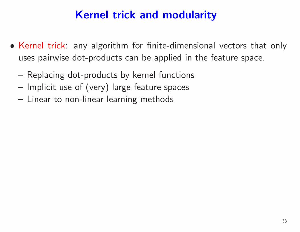
Kernel trick and modularity
• Kernel trick: any algorithm for finite-dimensional vectors that only
uses pairwise dot-products can be applied in the feature space.
– Replacing dot-products by kernel functions
– Implicit use of (very) large feature spaces
– Linear to non-linear learning methods
38

Kernel trick and modularity
• Kernel trick: any algorithm for finite-dimensional vectors that only
uses pairwise dot-products can be applied in the feature space.
– Replacing dot-products by kernel functions
– Implicit use of (very) large feature spaces
– Linear to non-linear learning methods
• Modularity of kernel methods
1. Work on new algorithms and theoretical analysis
2. Work on new kernels for specific data types
39

Representer theorem and convex duality
• The parameters α ∈ Rn may also be interpreted as Lagrange
multipliers
• Assumption: cost function is convex, ϕi(ui) = ℓ(yi, ui)
• Primal problem: minf∈F
∑ni=1ϕi(f
⊤Φ(xi)) +λ2‖f‖2
• What about the constant term b? replace Φ(x) by (Φ(x), c), c large
ϕi(ui)
LS regression 12(yi − ui)2
Logistic
regressionlog(1 + exp(−yiui))
SVM (1− yiui)+40

Representer theorem and convex duality
Proof
• Primal problem: minf∈F
∑ni=1ϕi(f
⊤Φ(xi)) +λ2‖f‖2
• Define ψi(vi) = maxui∈R
viui − ϕi(ui) as the Fenchel conjugate of ϕi
• Main trick: introduce constraint ui = f⊤Φ(xi) and associated
Lagrange multipliers αi
• Lagrangian L(α, f) =n∑
i=1
ϕi(ui) +λ
2‖f‖2 + λ
n∑
i=1
αi(ui − f⊤Φ(xi))
– Maximize with respect to ui ⇒ term of the form −ψi(−λαi)
– Maximize with respect to f ⇒ f =∑n
i=1αiΦ(xi)
41

Representer theorem and convex duality
• Assumption: cost function is convex ϕi(ui) = ℓ(yi, ui)
• Primal problem: minf∈F
∑ni=1ϕi(f
⊤Φ(xi)) +λ2‖f‖2
• Dual problem: maxα∈Rn
−∑ni=1ψi(−λαi)− λ
2α⊤Kα
where ψi(vi) = maxui∈R viui−ϕi(ui) is the Fenchel conjugate of ϕi
• Strong duality
• Relationship between primal and dual variables (at optimum):
f =∑n
i=1αiΦ(xi)
• NB: adding constant term b ⇔ add constraints∑n
i=1αi = 0
42
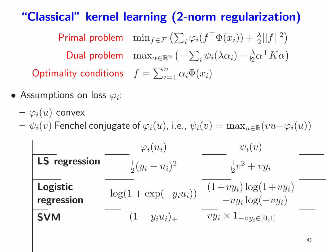
“Classical” kernel learning (2-norm regularization)
Primal problem minf∈F(∑
iϕi(f⊤Φ(xi)) +
λ2 ||f ||2
)
Dual problem maxα∈Rn
(−∑iψi(λαi)− λ
2α⊤Kα
)
Optimality conditions f =∑n
i=1αiΦ(xi)
• Assumptions on loss ϕi:
– ϕi(u) convex
– ψi(v) Fenchel conjugate of ϕi(u), i.e., ψi(v) = maxu∈R(vu−ϕi(u))
ϕi(ui) ψi(v)
LS regression 12(yi − ui)2 1
2v2 + vyi
Logistic
regressionlog(1 + exp(−yiui))
(1+vyi) log(1+vyi)
−vyi log(−vyi)SVM (1− yiui)+ vyi × 1−vyi∈[0,1]
43
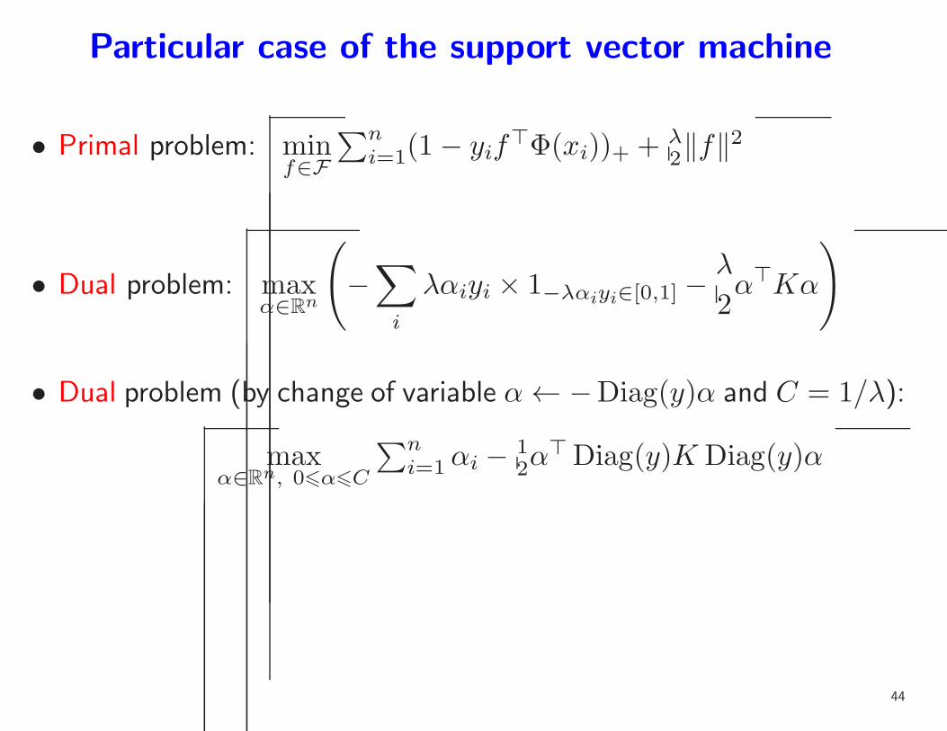
Particular case of the support vector machine
• Primal problem: minf∈F
∑ni=1(1− yif⊤Φ(xi))+ + λ
2‖f‖2
• Dual problem: maxα∈Rn
(
−∑
i
λαiyi × 1−λαiyi∈[0,1] −λ
2α⊤Kα
)
• Dual problem (by change of variable α← −Diag(y)α and C = 1/λ):
maxα∈Rn, 06α6C
∑ni=1αi − 1
2α⊤Diag(y)K Diag(y)α
44

Particular case of the support vector machine
• Primal problem: minf∈F
∑ni=1(1− yif⊤Φ(xi))+ + λ
2‖f‖2
• Dual problem:
maxα∈Rn, 06α6C
∑ni=1αi − 1
2α⊤Diag(y)K Diag(y)α
45

Particular case of the support vector machine
• Primal problem: minf∈F
∑ni=1(1− yif⊤Φ(xi))+ + λ
2‖f‖2
• Dual problem:
maxα∈Rn, 06α6C
∑ni=1αi − 1
2α⊤Diag(y)K Diag(y)α
• What about the traditional picture?
46

Course outline
1. Losses for particular machine learning tasks
• Classification, regression, etc...
2. Regularization by Hilbertian norms (kernel methods)
• Kernels and representer theorem
• Convex duality, optimization and algorithms
• Kernel methods
• Kernel design
3. Regularization by sparsity-inducing norms
• ℓ1-norm regularization
• Multiple kernel learning
• Theoretical results
• Learning on matrices
47

Kernel ridge regression (a.k.a. spline smoothing) - I
• Data x1, . . . , xn ∈ X , p.d. kernel k, y1, . . . , yn ∈ R
• Least-squares
minf∈F
1
n
n∑
i=1
(yi − f(xi))2 + λ‖f‖2F
• View 1: representer theorem ⇒ f =∑n
i=1αik(·, xi)– equivalent to
minα∈Rn
1
n
n∑
i=1
(yi − (Kα)i)2 + λα⊤Kα
– Solution equal to α = (K + nλI)−1y + ε with Kε = 0
– Unique solution f
48

Kernel ridge regression (a.k.a. spline smoothing) - II
• Links with spline smoothing (Wahba, 1990)
• Other view: F ∈ Rd, Φ ∈ R
n×d
minw∈Rd
1
n‖y − Φw‖2 + λ‖w‖2
• Solution equal to w = (Φ⊤Φ+ nλI)−1Φ⊤y
• Note that w = Φ⊤(ΦΦ⊤ + nλI)−1y
– Using matrix inversion lemma
• Φw equal to Kα
49

Kernel ridge regression (a.k.a. spline smoothing) - III
• Dual view:
– dual problem: maxα∈Rn−nλ2 ‖α‖2 − α⊤y − 1
2α⊤Kα
– solution: α = (K + λI)−1y
• Warning: same solution obtained from different point of views
50

Losses for classification
• Usual convex costs:
−3 −2 −1 0 1 2 3 40
1
2
3
4
5
0−1hingesquarelogistic
• Differences between hinge and logistic loss: differentiability/sparsity
51

Support vector machine or logistic regression?
• Predictive performance is similar
• Only true difference is numerical
– SVM: sparsity in α
– Logistic: differentiable loss function
• Which one to use?
– Linear kernel ⇒ Logistic + Newton/Gradient descent
– Linear kernel - Large scale ⇒ Stochastic gradient descent
– Nonlinear kernel ⇒ SVM + dual methods or simpleSVM
52

Algorithms for supervised kernel methods
• Four formulations
1. Dual: maxα∈Rn−∑iψi(λαi)− λ2α
⊤Kα2. Primal: minf∈F
∑
iϕi(f⊤Φ(xi)) +
λ2 ||f ||2
3. Primal + Representer: minα∈Rn∑
iϕi((Kα)i) +λ2α
⊤Kα4. Convex programming
• Best strategy depends on loss (differentiable or not) and kernel
(linear or not)
53

Dual methods
• Dual problem: maxα∈Rn−∑iψi(λαi)− λ2α
⊤Kα
• Main method: coordinate descent (a.k.a. sequential minimal
optimization - SMO) (Platt, 1998; Bottou and Lin, 2007; Joachims,
1998)
– Efficient when loss is piecewise quadratic (i.e., hinge = SVM)
– Sparsity may be used in the case of the SVM
• Computational complexity: between quadratic and cubic in n
• Works for all kernels
54

Primal methods
• Primal problem: minf∈F∑
iϕi(f⊤Φ(xi)) +
λ2 ||f ||2
• Only works directly if Φ(x) may be built explicitly and has small
dimension
– Example: linear kernel in small dimensions
• Differentiable loss: gradient descent or Newton’s method are very
efficient in small dimensions
• Larger scale
– stochastic gradient descent (Shalev-Shwartz et al., 2007; Bottou
and Bousquet, 2008)
– See Leon Bottou’s course
55

Primal methods with representer theorems
• Primal problem in α: minα∈Rn∑
iϕi((Kα)i) +λ2α
⊤Kα
• Direct optimization in α poorly conditioned (K has low-rank) unless
Newton method is used (Chapelle, 2007)
• General kernels: use incomplete Cholesky decomposition (Fine and
Scheinberg, 2001; Bach and Jordan, 2002) to obtain a square root
K = GG⊤
K
T
=G
GG of size n×m,
where m≪ n
– “Empirical input space” of size m obtained using rows of G
– Running time to compute G: O(m2n)
56

Direct convex programming
• Convex programming toolboxes ⇒ very inefficient!
• May use special structure of the problem
– e.g., SVM and sparsity in α
• Active set method for the SVM: SimpleSVM (Vishwanathan et al.,
2003; Loosli et al., 2005)
– Cubic complexity in the number of support vectors
• Full regularization path for the SVM (Hastie et al., 2005; Bach et al.,
2006)
– Cubic complexity in the number of support vectors
– May be extended to other settings (Rosset and Zhu, 2007)
57

Code
• SVM and other supervised learning techniques
www.shogun-toolbox.org
http://gaelle.loosli.fr/research/tools/simplesvm.html
http://www.kyb.tuebingen.mpg.de/bs/people/spider/main.html
http://ttic.uchicago.edu/~shai/code/index.html
• ℓ1-penalization:– SPAMS (SPArse Modeling Software)
http://www.di.ens.fr/willow/SPAMS/
• Multiple kernel learning:
asi.insa-rouen.fr/enseignants/~arakotom/code/mklindex.html
www.stat.berkeley.edu/~gobo/SKMsmo.tar
58

Course outline
1. Losses for particular machine learning tasks
• Classification, regression, etc...
2. Regularization by Hilbertian norms (kernel methods)
• Kernels and representer theorem
• Convex duality, optimization and algorithms
• Kernel methods
• Kernel design
3. Regularization by sparsity-inducing norms
• ℓ1-norm regularization
• Multiple kernel learning
• Theoretical results
• Learning on matrices
59

Kernel methods - I
• Distances in the “feature space”
dk(x, y)2 = ‖Φ(x)− Φ(y)‖2F = k(x, x) + k(y, y)− 2k(x, y)
• Nearest-neighbor classification/regression
60

Kernel methods - II
Simple discrimination algorithm
• Data x1, . . . , xn ∈ X , classes y1, . . . , yn ∈ −1, 1
• Compare distances to mean of each class
• Equivalent to classifying x using the sign of
1
#i, yi = 1∑
i,yi=1
k(x, xi)−1
#i, yi = −1∑
i,yi=−1
k(x, xi)
• Proof...
• Geometric interpretation of Parzen windows
61

Kernel methods - III
Data centering
• n points x1, . . . , xn ∈ X
• kernel matrix K ∈ Rn, Kij = k(xi, xj) = 〈Φ(xi),Φ(xj)〉
• Kernel matrix of centered data Kij = 〈Φ(xi)− µ,Φ(xj)− µ〉where µ = 1
n
∑ni=1Φ(xi)
• Formula: K = ΠnKΠn with Πn = In − En , and E constant matrix
equal to 1.
• Proof...
• NB: µ is not of the form Φ(z), z ∈ X (cf. preimage problem)
62

Kernel PCA
• Linear principal component analysis
– data x1, . . . , xn ∈ Rp,
maxw∈Rp
w⊤Σw
w⊤w= max
w∈Rp
var(w⊤X)
w⊤w
– w is largest eigenvector of Σ
– Denoising, data representation
• Kernel PCA: data x1, . . . , xn ∈ X , p.d. kernel k
– View 1: maxw∈F
var(〈Φ(X), w〉)w⊤w
View 2: maxf∈F
var(f(X))
‖f‖2F– Solution: f,w =
∑ni=1αik(·, xi) and α first eigenvector of K =
ΠnKΠn
– Interpretation in terms of covariance operators
63

Denoising with kernel PCA (From Scholkopf, 2005)
64

Canonical correlation analysis
x1 x2ξ1 ξ2
• Given two multivariate random variables x1 and x2, finds the pair of
directions ξ1, ξ2 with maximum correlation:
ρ(x1, x2) = maxξ1,ξ2
corr(ξT1 x1, ξT2 x2) = max
ξ1,ξ2
ξT1 C12ξ2(ξT1 C11ξ1
)1/2 (ξT2 C22ξ2
)1/2
• Generalized eigenvalue problem:
(0 C12
C21 0
)(ξ1ξ2
)
= ρ
(C11 0
0 C22
)(ξ1ξ2
)
.
65
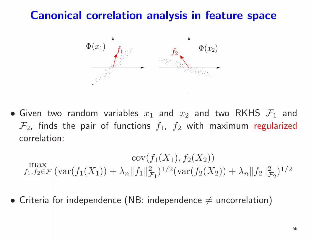
Canonical correlation analysis in feature space
f1 f2Φ(x1) Φ(x2)
• Given two random variables x1 and x2 and two RKHS F1 and
F2, finds the pair of functions f1, f2 with maximum regularized
correlation:
maxf1,f2∈F
cov(f1(X1), f2(X2))
(var(f1(X1)) + λn‖f1‖2F1)1/2(var(f2(X2)) + λn‖f2‖2F2
)1/2
• Criteria for independence (NB: independence 6= uncorrelation)
66

Kernel Canonical Correlation Analysis
• Analogous derivation as Kernel PCA
• K1, K2 Gram matrices of xi1 and xi2
maxα1, α2∈ℜN
αT1K1K2α2
(αT1 (K
21 + λK1)α1)1/2(αT
2 (K22 + λK2)α2)1/2
• Maximal generalized eigenvalue of
(0 K1K2
K2K1 0
)(α1
α2
)
= ρ
(K2
1 + λK1 0
0 K22 + λK2
)(α1
α2
)
67

Kernel CCA
Application to ICA (Bach & Jordan, 2002)
• Independent component analysis: linearly transform data such to get
independent variables
Sources
x1
x2Mixtures
y1
y2
WhitenedMixtures
y1~
y2~
ICAProjections
y1~
y2~
68

Empirical results - Kernel ICA
• Comparison with other algorithms: FastICA (Hyvarinen,1999), Jade
(Cardoso, 1998), Extended Infomax (Lee, 1999)
• Amari error : standard ICA distance from true sources
0
0.1
0.2
0.3
0
0.1
0.2
0.3
0
0.1
0.2
0.3
Randompdfs
Randompdfs
Randompdfs
Randompdfs
0
0.1
0.2
0.3
KGV KCCA FastICA JADE IMAX
69

Course outline
1. Losses for particular machine learning tasks
• Classification, regression, etc...
2. Regularization by Hilbertian norms (kernel methods)
• Kernels and representer theorem
• Convex duality, optimization and algorithms
• Kernel methods
• Kernel design
3. Regularization by sparsity-inducing norms
• ℓ1-norm regularization
• Multiple kernel learning
• Theoretical results
• Learning on matrices
70

Kernel design
• Principle: kernel on X = space of functions on X + norm
• Two main design principles
1. Constructing kernels from kernels by algebraic operations
2. Using usual algebraic/numerical tricks to perform efficient kernel
computation with very high-dimensional feature spaces
• Operations: k1(x, y)=〈Φ1(x),Φ1(y)〉, k2(x, y)=〈Φ2(x),Φ2(y)〉– Sum = concatenation of feature spaces:
k1(x, y) + k2(x, y) =⟨(Φ1(x)
Φ2(x)
),(Φ1(y)Φ2(y)
)⟩
– Product = tensor product of feature spaces:
k1(x, y)k2(x, y) =⟨Φ1(x)Φ2(x)
⊤,Φ1(y)Φ2(y)⊤⟩
71

Classical kernels: kernels on vectors x ∈ Rd
• Linear kernel k(x, y) = x⊤y
– Linear functions
• Polynomial kernel k(x, y) = (1 + x⊤y)d
– Polynomial functions
• Gaussian kernel k(x, y) = exp(−α‖x− y‖2)– Smooth functions
• Data are not always vectors!
72

Efficient ways of computing large sums
• Goal: Φ(x) ∈ Rp high-dimensional, compute
p∑
i=1
Φi(x)Φi(y) in o(p)
• Sparsity: many Φi(x) equal to zero (example: pyramid match kernel)
• Factorization and recursivity: replace sums of many products by
product of few sums (example: polynomial kernel, graph kernel)
(1 + x⊤y)d =∑
α1+···+αk6d
(d
α1, . . . , αk
)
(x1y1)α1 · · · (xkyk)αk
73

Kernels over (labelled) sets of points
• Common situation in computer vision (e.g., interest points)
• Simple approach: compute averages/histograms of certain features
– valid kernels over histograms h and h′ (Hein and Bousquet, 2004)
– intersection:∑
imin(hi, h′i), chi-square: exp
(
−α∑i(hi−h′
i)2
hi+h′i
)
74

Kernels over (labelled) sets of points
• Common situation in computer vision (e.g., interest points)
• Simple approach: compute averages/histograms of certain features
– valid kernels over histograms h and h′ (Hein and Bousquet, 2004)
– intersection:∑
imin(hi, h′i), chi-square: exp
(
−α∑i(hi−h′
i)2
hi+h′i
)
• Pyramid match (Grauman and Darrell, 2007): efficiently introducing
localization
– Form a regular pyramid on top of the image
– Count the number of common elements in each bin
– Give a weight to each bin
– Many bins but most of them are empty
⇒ use sparsity to compute kernel efficiently
75

Pyramid match kernel
(Grauman and Darrell, 2007; Lazebnik et al., 2006)
• Two sets of points
• Counting matches at several scales: 7, 5, 4
76

Kernels from segmentation graphs
• Goal of segmentation: extract objects of interest
• Many methods available, ....
– ... but, rarely find the object of interest entirely
• Segmentation graphs
– Allows to work on “more reliable” over-segmentation
– Going to a large square grid (millions of pixels) to a small graph
(dozens or hundreds of regions)
• How to build a kernel over segmenation graphs?
– NB: more generally, kernelizing existing representations?
77

Segmentation by watershed transform (Meyer, 2001)
image gradient watershed
287 segments 64 segments 10 segments
78

Segmentation by watershed transform (Meyer, 2001)
image gradient watershed
287 segments 64 segments 10 segments
79

Image as a segmentation graph
• Labelled undirected graph
– Vertices: connected segmented regions
– Edges: between spatially neighboring regions
– Labels: region pixels
⇒
80

Image as a segmentation graph
• Labelled undirected graph
– Vertices: connected segmented regions
– Edges: between spatially neighboring regions
– Labels: region pixels
• Difficulties
– Extremely high-dimensional labels
– Planar undirected graph
– Inexact matching
• Graph kernels (Gartner et al., 2003; Kashima et al., 2004; Harchaoui
and Bach, 2007) provide an elegant and efficient solution
81

Kernels between structured objects
Strings, graphs, etc... (Shawe-Taylor and Cristianini, 2004)
• Numerous applications (text, bio-informatics, speech, vision)
• Common design principle: enumeration of subparts (Haussler,
1999; Watkins, 1999)
– Efficient for strings
– Possibility of gaps, partial matches, very efficient algorithms
• Most approaches fails for general graphs (even for undirected trees!)
– NP-Hardness results (Ramon and Gartner, 2003)
– Need specific set of subparts
82

Paths and walks
• Given a graph G,
– A path is a sequence of distinct neighboring vertices
– A walk is a sequence of neighboring vertices
• Apparently similar notions
83

Paths
84

Walks
85

Walk kernel (Kashima et al., 2004; Borgwardt et al., 2005)
• WpG (resp. Wp
H) denotes the set of walks of length p in G (resp. H)
• Given basis kernel on labels k(ℓ, ℓ′)
• p-th order walk kernel:
kpW(G,H) =∑
(r1, . . . , rp) ∈ WpG
(s1, . . . , sp) ∈ WpH
p∏
i=1
k(ℓG(ri), ℓH(si)).
G
1
s3
2s
s 1r2
3rH
r
86
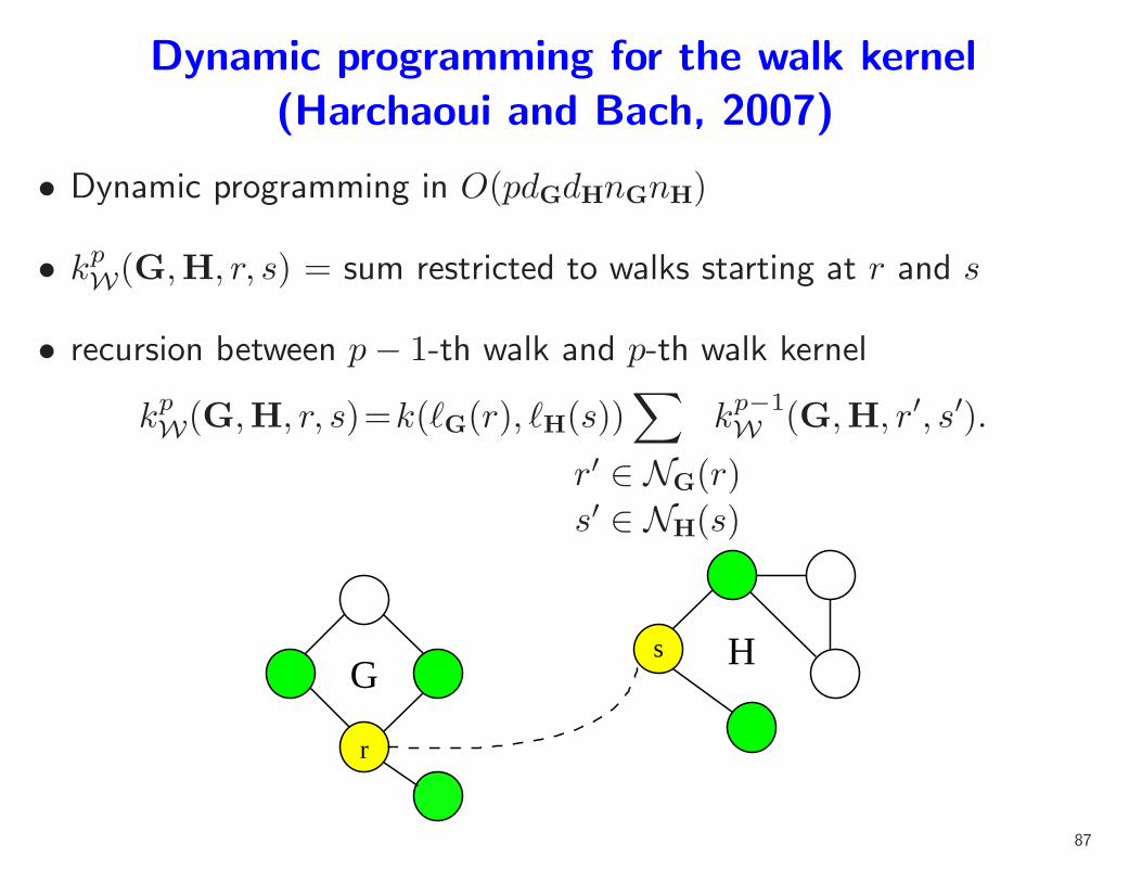
Dynamic programming for the walk kernel
(Harchaoui and Bach, 2007)
• Dynamic programming in O(pdGdHnGnH)
• kpW(G,H, r, s) = sum restricted to walks starting at r and s
• recursion between p− 1-th walk and p-th walk kernel
kpW(G,H, r, s)=k(ℓG(r), ℓH(s))∑
r′ ∈ NG(r)
s′ ∈ NH(s)
kp−1W (G,H, r′, s′).
Gs
r
H
87

Dynamic programming for the walk kernel
(Harchaoui and Bach, 2007)
• Dynamic programming in O(pdGdHnGnH)
• kpW(G,H, r, s) = sum restricted to walks starting at r and s
• recursion between p− 1-th walk and p-th walk kernel
kpW(G,H, r, s)=k(ℓG(r), ℓH(s))∑
r′ ∈ NG(r)
s′ ∈ NH(s)
kp−1W (G,H, r′, s′)
• Kernel obtained as kp,αT (G,H) =∑
r∈VG,s∈VH
kp,αT (G,H, r, s)
88

Extensions of graph kernels
• Main principle: compare all possible subparts of the graphs
• Going from paths to subtrees
– Extension of the concept of walks ⇒ tree-walks (Ramon and
Gartner, 2003)
• Similar dynamic programming recursions (Harchaoui and Bach, 2007)
• Need to play around with subparts to obtain efficient recursions
– Do we actually need positive definiteness?
89

Performance on Corel14 (Harchaoui and Bach, 2007)
• Corel14: 1400 natural images with 14 classes
90

Performance on Corel14 (Harchaoui & Bach, 2007)
Error rates
• Histogram kernels (H)
• Walk kernels (W)
• Tree-walk kernels (TW)
• Weighted tree-walks(wTW)
• MKL (M) H W TW wTW M
0.05
0.06
0.07
0.08
0.09
0.1
0.11
0.12
Tes
t err
or
Kernels
Performance comparison on Corel14
91
Kernel methods - Summary
• Kernels and representer theorems
– Clear distinction between representation/algorithms
• Algorithms
– Two formulations (primal/dual)
– Logistic or SVM?
• Kernel design
– Very large feature spaces with efficient kernel evaluations
92
Course outline
1. Losses for particular machine learning tasks
• Classification, regression, etc...
2. Regularization by Hilbertian norms (kernel methods)
• Kernels and representer theorem
• Convex duality, optimization and algorithms
• Kernel methods
• Kernel design
3. Regularization by sparsity-inducing norms
• ℓ1-norm regularization
• Multiple kernel learning
• Theoretical results
• Learning on matrices
93

Supervised learning and regularization
• Data: xi ∈ X , yi ∈ Y, i = 1, . . . , n
• Minimize with respect to function f : X → Y:n∑
i=1
ℓ(yi, f(xi)) +λ
2‖f‖2
Error on data + Regularization
Loss & function space ? Norm ?
• Two theoretical/algorithmic issues:
1. Loss
2. Function space / norm
94

Regularizations
• Main goal: avoid overfitting
• Two main lines of work:
1. Euclidean and Hilbertian norms (i.e., ℓ2-norms)
– Possibility of non linear predictors
– Non parametric supervised learning and kernel methods
– Well developped theory and algorithms (see, e.g., Wahba, 1990;
Scholkopf and Smola, 2001; Shawe-Taylor and Cristianini, 2004)
95

Regularizations
• Main goal: avoid overfitting
• Two main lines of work:
1. Euclidean and Hilbertian norms (i.e., ℓ2-norms)
– Possibility of non linear predictors
– Non parametric supervised learning and kernel methods
– Well developped theory and algorithms (see, e.g., Wahba, 1990;
Scholkopf and Smola, 2001; Shawe-Taylor and Cristianini, 2004)
2. Sparsity-inducing norms
– Usually restricted to linear predictors on vectors f(x) = w⊤x– Main example: ℓ1-norm ‖w‖1 =
∑pi=1 |wi|
– Perform model selection as well as regularization
– Theory and algorithms “in the making”
96

ℓ2-norm vs. ℓ1-norm
• ℓ1-norms lead to interpretable models
• ℓ2-norms can be run implicitly with very large feature spaces
• Algorithms:
– Smooth convex optimization vs. nonsmooth convex optimization
• Theory:
– better predictive performance?
97

ℓ2 vs. ℓ1 - Gaussian hare vs. Laplacian tortoise
• First-order methods (Fu, 1998; Wu and Lange, 2008)• Homotopy methods (Markowitz, 1956; Efron et al., 2004)
98

Lasso - Two main recent theoretical results
1. Support recovery condition (Zhao and Yu, 2006; Wainwright, 2006;
Zou, 2006; Yuan and Lin, 2007): the Lasso is sign-consistent if and
only if
‖QJcJQ−1JJ sign(wJ)‖∞ 6 1,
where Q = limn→+∞1n
∑ni=1 xix
⊤i ∈ R
p×p and J = Supp(w)
99

Lasso - Two main recent theoretical results
1. Support recovery condition (Zhao and Yu, 2006; Wainwright, 2006;
Zou, 2006; Yuan and Lin, 2007): the Lasso is sign-consistent if and
only if
‖QJcJQ−1JJ sign(wJ)‖∞ 6 1,
where Q = limn→+∞1n
∑ni=1 xix
⊤i ∈ R
p×p and J = Supp(w)
2. Exponentially many irrelevant variables (Zhao and Yu, 2006;
Wainwright, 2006; Bickel et al., 2009; Lounici, 2008; Meinshausen
and Yu, 2008): under appropriate assumptions, consistency is possible
as long as
log p = O(n)
100

Going beyond the Lasso
• ℓ1-norm for linear feature selection in high dimensions
– Lasso usually not applicable directly
• Non-linearities
• Dealing with exponentially many features
• Sparse learning on matrices
101

Why ℓ1-norm constraints leads to sparsity?
• Example: minimize quadratic function Q(w) subject to ‖w‖1 6 T .
– coupled soft thresholding
• Geometric interpretation
– NB : penalizing is “equivalent” to constraining
1
2w
w 1
2w
w
102

ℓ1-norm regularization (linear setting)
• Data: covariates xi ∈ Rp, responses yi ∈ Y, i = 1, . . . , n
• Minimize with respect to loadings/weights w ∈ Rp:
J(w) =n∑
i=1
ℓ(yi, w⊤xi) + λ‖w‖1
Error on data + Regularization
• Including a constant term b? Penalizing or constraining?
• square loss ⇒ basis pursuit in signal processing (Chen et al., 2001),
Lasso in statistics/machine learning (Tibshirani, 1996)
103

First order methods for convex optimization on Rp
Smooth optimization
• Gradient descent: wt+1 = wt − αt∇J(wt)
– with line search: search for a decent (not necessarily best) αt
– fixed diminishing step size, e.g., αt = a(t+ b)−1
• Convergence of f(wt) to f∗ = minw∈Rp f(w) (Nesterov, 2003)
– f convex andM -Lipschitz: f(wt)−f∗ = O(M/√t)
– and, differentiable with L-Lipschitz gradient: f(wt)−f∗ = O(L/t)
– and, f µ-strongly convex: f(wt)−f∗ = O(L exp(−4tµL)
)
• µL = condition number of the optimization problem
• Coordinate descent: similar properties
• NB: “optimal scheme” f(wt)−f∗ = O(Lminexp(−4t
√
µ/L), t−2)
104

First-order methods for convex optimization on Rp
Non smooth optimization
• First-order methods for non differentiable objective
– Subgradient descent: wt+1 = wt − αtgt, with gt ∈ ∂J(wt)
∗ with exact line search: not always convergent (see counter-
example)
∗ diminishing step size, e.g., αt = a(t+ b)−1: convergent
– Coordinate descent: not always convergent (show counter-example)
• Convergence rates (f convex andM -Lipschitz): f(wt)−f∗ = O(M√t
)
105

Counter-example
Coordinate descent for nonsmooth objectives
54
32
1
w
w2
1
106

Counter-example (Bertsekas, 1995)
Steepest descent for nonsmooth objectives
• q(x1, x2) = −5(9x21 + 16x22)
1/2 if x1 > |x2|−(9x1 + 16|x2|)1/2 if x1 6 |x2|
• Steepest descent starting from any x such that x1 > |x2| >(9/16)2|x1|
−5 0 5−5
0
5
107

Regularized problems - Proximal methods
• Gradient descent as a proximal method (differentiable functions)
– wt+1 = arg minw∈Rp
J(wt) + (w − wt)⊤∇J(wt)+
L
2‖w − wt‖22
– wt+1 = wt − 1L∇J(wt)
• Problems of the form: minw∈Rp
L(w) + λΩ(w)
– wt+1 = arg minw∈Rp
L(wt)+(w−wt)⊤∇L(wt)+λΩ(w)+
L
2‖w − wt‖22
– Thresholded gradient descent
• Similar convergence rates than smooth optimization
– Acceleration methods (Nesterov, 2007; Beck and Teboulle, 2009)
– depends on the condition number of the loss
108

Second order methods
• Differentiable case
– Newton: wt+1 = wt − αtH−1t gt
∗ Traditional: αt = 1, but non globally convergent
∗ globally convergent with line search for αt (see Boyd, 2003)
∗ O(log log(1/ε)) (slower) iterations
– Quasi-newton methods (see Bonnans et al., 2003)
• Non differentiable case (interior point methods)
– Smoothing of problem + second order methods
∗ See example later and (Boyd, 2003)
∗ Theoretically O(√p) Newton steps, usually O(1) Newton steps
109

First order or second order methods for machine
learning?
• objecive defined as average (i.e., up to n−1/2): no need to optimize
up to 10−16!
– Second-order: slower but worryless
– First-order: faster but care must be taken regarding convergence
• Rule of thumb
– Small scale ⇒ second order
– Large scale ⇒ first order
– Unless dedicated algorithm using structure (like for the Lasso)
• See Bottou and Bousquet (2008) for further details
110

Piecewise linear paths
0 0.1 0.2 0.3 0.4 0.5 0.6
−0.6
−0.4
−0.2
0
0.2
0.4
0.6
regularization parameter
wei
ghts
111

Algorithms for ℓ1-norms (square loss):
Gaussian hare vs. Laplacian tortoise
• Coordinate descent: O(pn) per iterations for ℓ1 and ℓ2
• “Exact” algorithms: O(kpn) for ℓ1 vs. O(p2n) for ℓ2
112

Additional methods - Softwares
• Many contributions in signal processing, optimization, machine
learning
– Extensions to stochastic setting (Bottou and Bousquet, 2008)
• Extensions to other sparsity-inducing norms
– Computing proximal operator
– See http://www.di.ens.fr/~fbach/opt_book.pdf
• Softwares
– Many available codes
– SPAMS (SPArse Modeling Software)
http://www.di.ens.fr/willow/SPAMS/
113

Course outline
1. Losses for particular machine learning tasks
• Classification, regression, etc...
2. Regularization by Hilbertian norms (kernel methods)
• Kernels and representer theorem
• Convex duality, optimization and algorithms
• Kernel methods
• Kernel design
3. Regularization by sparsity-inducing norms
• ℓ1-norm regularization
• Multiple kernel learning
• Theoretical results
• Learning on matrices
114

Theoretical results - Square loss
• Main assumption: data generated from a certain sparse w
• Three main problems:
1. Regular consistency: convergence of estimator w to w, i.e.,
‖w −w‖ tends to zero when n tends to ∞2. Model selection consistency: convergence of the sparsity pattern
of w to the pattern w
3. Efficiency: convergence of predictions with w to the predictions
with w, i.e., 1n‖Xw −Xw‖22 tends to zero
• Main results:
– Condition for model consistency (support recovery)
– High-dimensional inference
115

Model selection consistency (Lasso)
• Assume w sparse and denote J = j,wj 6= 0 the nonzero pattern
• Support recovery condition (Zhao and Yu, 2006; Wainwright, 2006;
Zou, 2006; Yuan and Lin, 2007): the Lasso is sign-consistent if and
only if ‖QJcJQ−1JJ sign(wJ)‖∞ 6 1
where Q = limn→+∞1n
∑ni=1 xix
⊤i ∈ R
p×p and J = Supp(w)
116

Model selection consistency (Lasso)
• Assume w sparse and denote J = j,wj 6= 0 the nonzero pattern
• Support recovery condition (Zhao and Yu, 2006; Wainwright, 2006;
Zou, 2006; Yuan and Lin, 2007): the Lasso is sign-consistent if and
only if ‖QJcJQ−1JJ sign(wJ)‖∞ 6 1
where Q = limn→+∞1n
∑ni=1 xix
⊤i ∈ R
p×p and J = Supp(w)
• Condition depends on w and J (may be relaxed)
– may be relaxed by maximizing out sign(w) or J
• Valid in low and high-dimensional settings
• Requires lower-bound on magnitude of nonzero wj
117

Model selection consistency (Lasso)
• Assume w sparse and denote J = j,wj 6= 0 the nonzero pattern
• Support recovery condition (Zhao and Yu, 2006; Wainwright, 2006;
Zou, 2006; Yuan and Lin, 2007): the Lasso is sign-consistent if and
only if ‖QJcJQ−1JJ sign(wJ)‖∞ 6 1
where Q = limn→+∞1n
∑ni=1 xix
⊤i ∈ R
p×p and J = Supp(w)
• The Lasso is usually not model-consistent
– Selects more variables than necessary (see, e.g., Lv and Fan, 2009)
– Fixing the Lasso: adaptive Lasso (Zou, 2006), relaxed
Lasso (Meinshausen, 2008), thresholding (Lounici, 2008),
Bolasso (Bach, 2008a), stability selection (Meinshausen and
Buhlmann, 2008), Wasserman and Roeder (2009)
118

Adaptive Lasso and concave penalization
• Adaptive Lasso (Zou, 2006; Huang et al., 2008)
– Weighted ℓ1-norm: minw∈Rp
L(w) + λ
p∑
j=1
|wj||wj|α
– w estimator obtained from ℓ2 or ℓ1 regularization
• Reformulation in terms of concave penalization
minw∈Rp
L(w) +
p∑
j=1
g(|wj|)
– Example: g(|wj|) = |wj|1/2 or log |wj|. Closer to the ℓ0 penalty
– Concave-convex procedure: replace g(|wj|) by affine upper bound
– Better sparsity-inducing properties (Fan and Li, 2001; Zou and Li,
2008; Zhang, 2008b)
119

High-dimensional inference (Lasso)
• Main result: we only need k log p = O(n)
– if w is sufficiently sparse
– and input variables are not too correlated
• Precise conditions on covariance matrix Q = 1nX
⊤X.
– Mutual incoherence (Lounici, 2008)
– Restricted eigenvalue conditions (Bickel et al., 2009)
– Sparse eigenvalues (Meinshausen and Yu, 2008)
– Null space property (Donoho and Tanner, 2005)
• Links with signal processing and compressed sensing (Candes and
Wakin, 2008)
• Assume that Q has unit diagonal
120

Mutual incoherence (uniform low correlations)
• Theorem (Lounici, 2008):
– yi = w⊤xi + εi, ε i.i.d. normal with mean zero and variance σ2
– Q = X⊤X/n with unit diagonal and cross-terms less than1
14k– if ‖w‖0 6 k, and A2 > 8, then, with λ = Aσ
√n log p
P
(
‖w −w‖∞ 6 5Aσ
(log p
n
)1/2)
> 1− p1−A2/8
• Model consistency by thresholding if minj,wj 6=0
|wj| > Cσ
√
log p
n
• Mutual incoherence condition depends strongly on k
• Improved result by averaging over sparsity patterns (Candes and Plan,
2009)
121

Alternative sparse methods
Greedy methods
• Forward selection
• Forward-backward selection
• Non-convex method
– Harder to analyze
– Simpler to implement
– Problems of stability
• Positive theoretical results (Zhang, 2009, 2008a)
– Similar sufficient conditions than for the Lasso
122

Comparing Lasso and other strategies for linear
regression
• Compared methods to reach the least-square solution
– Ridge regression: minw∈Rp
1
2‖y −Xw‖22 +
λ
2‖w‖22
– Lasso: minw∈Rp
1
2‖y −Xw‖22 + λ‖w‖1
– Forward greedy:
∗ Initialization with empty set
∗ Sequentially add the variable that best reduces the square loss
• Each method builds a path of solutions from 0 to ordinary least-
squares solution
• Regularization parameters selected on the test set
123

Simulation results
• i.i.d. Gaussian design matrix, k = 4, n = 64, p ∈ [2, 256], SNR = 1
• Note stability to non-sparsity and variability
2 4 6 80
0.1
0.2
0.3
0.4
0.5
0.6
0.7
0.8
0.9
log2(p)
mea
n sq
uare
err
or
L1L2greedyoracle
2 4 6 80
0.1
0.2
0.3
0.4
0.5
0.6
0.7
0.8
0.9
log2(p)
mea
n sq
uare
err
or
L1L2greedy
Sparse Rotated (non sparse)
124

Summary
ℓ1-norm regularization
• ℓ1-norm regularization leads to nonsmooth optimization problems
– analysis through directional derivatives or subgradients
– optimization may or may not take advantage of sparsity
• ℓ1-norm regularization allows high-dimensional inference
• Interesting problems for ℓ1-regularization
– Stable variable selection
– Weaker sufficient conditions (for weaker results)
– Estimation of regularization parameter (all bounds depend on the
unknown noise variance σ2)
125

Extensions
• Sparse methods are not limited to the square loss
– logistic loss: algorithms (Beck and Teboulle, 2009) and theory (Van
De Geer, 2008; Bach, 2009)
• Sparse methods are not limited to supervised learning
– Learning the structure of Gaussian graphical models (Meinshausen
and Buhlmann, 2006; Banerjee et al., 2008)
– Sparsity on matrices (last part of the tutorial)
• Sparse methods are not limited to variable selection in a linear
model
– See next part of the tutorial
126

Course outline
1. Losses for particular machine learning tasks
• Classification, regression, etc...
2. Regularization by Hilbertian norms (kernel methods)
• Kernels and representer theorem
• Convex duality, optimization and algorithms
• Kernel methods
• Kernel design
3. Regularization by sparsity-inducing norms
• ℓ1-norm regularization
• Multiple kernel learning
• Theoretical results
• Learning on matrices
127

Penalization with grouped variables
(Yuan and Lin, 2006)
• Assume that 1, . . . , p is partitioned into m groups G1, . . . , Gm
• Penalization by∑m
i=1 ‖wGi‖2, often called ℓ1-ℓ2 norm
• Induces group sparsity
– Some groups entirely set to zero
– no zeros within groups
• In this tutorial:
– Groups may have infinite size ⇒ MKL
– Groups may overlap⇒ structured sparsity (Jenatton et al., 2009)
128

Linear vs. non-linear methods
• All methods in this tutorial are linear in the parameters
• By replacing x by features Φ(x), they can be made non linear in
the data
• Implicit vs. explicit features
– ℓ1-norm: explicit features
– ℓ2-norm: representer theorem allows to consider implicit features if
their dot products can be computed easily (kernel methods)
129

Kernel methods: regularization by ℓ2-norm
• Data: xi ∈ X , yi ∈ Y, i = 1, . . . , n, with features Φ(x) ∈ F = Rp
– Predictor f(x) = w⊤Φ(x) linear in the features
• Optimization problem: minw∈Rp
n∑
i=1
ℓ(yi, w⊤Φ(xi)) +
λ
2‖w‖22
130

Kernel methods: regularization by ℓ2-norm
• Data: xi ∈ X , yi ∈ Y, i = 1, . . . , n, with features Φ(x) ∈ F = Rp
– Predictor f(x) = w⊤Φ(x) linear in the features
• Optimization problem: minw∈Rp
n∑
i=1
ℓ(yi, w⊤Φ(xi)) +
λ
2‖w‖22
• Representer theorem (Kimeldorf and Wahba, 1971): solution must
be of the form w =∑n
i=1αiΦ(xi)
– Equivalent to solving: minα∈Rn
n∑
i=1
ℓ(yi, (Kα)i) +λ
2α⊤Kα
– Kernel matrix Kij = k(xi, xj) = Φ(xi)⊤Φ(xj)
131

Multiple kernel learning (MKL)
(Lanckriet et al., 2004b; Bach et al., 2004a)
• Sparse methods are linear!
• Sparsity with non-linearities
– replace f(x) =∑p
j=1w⊤j xj with x ∈ R
p and wj ∈ R
– by f(x) =∑p
j=1w⊤j Φj(x) with x ∈ X , Φj(x) ∈ Fj an wj ∈ Fj
• Replace the ℓ1-norm∑p
j=1 |wj| by “block” ℓ1-norm∑p
j=1 ‖wj‖2
• Remarks
– Hilbert space extension of the group Lasso (Yuan and Lin, 2006)
– Alternative sparsity-inducing norms (Ravikumar et al., 2008)
132

Multiple kernel learning
• Learning combinations of kernels: K(η) =∑m
j=1 ηjKj, η > 0
– Summing kernels ⇔ concatenating feature spaces
– Assume k1(x, y)=〈Φ1(x),Φ1(y)〉, k2(x, y)=〈Φ2(x),Φ2(y)〉
k1(x, y) + k2(x, y) =⟨(Φ1(x)
Φ2(x)
),(Φ1(y)Φ2(y)
)⟩
• Summing kernels ⇔ generalized additive models
• Relationships with sparse additive models (Ravikumar et al., 2008)
133

Multiple kernel learning (MKL)
(Lanckriet et al., 2004b; Bach et al., 2004a)
• Multiple feature maps / kernels on x ∈ X :– p “feature maps” Φj : X 7→ Fj, j = 1, . . . , p.
– Minimization with respect to w1 ∈ F1, . . . , wp ∈ Fp
– Predictor: f(x) = w1⊤Φ1(x) + · · ·+ wp
⊤Φp(x)
x
Φ1(x)⊤ w1
ր ... ... ց−→ Φj(x)
⊤ wj −→ց ... ... ր
Φp(x)⊤ wp
w⊤1 Φ1(x) + · · ·+ w⊤
p Φp(x)
– Generalized additive models (Hastie and Tibshirani, 1990)
134
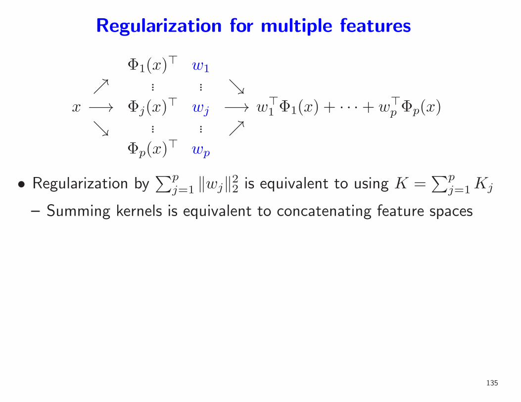
Regularization for multiple features
x
Φ1(x)⊤ w1
ր ... ... ց−→ Φj(x)
⊤ wj −→ց ... ... ր
Φp(x)⊤ wp
w⊤1 Φ1(x) + · · ·+ w⊤
p Φp(x)
• Regularization by∑p
j=1 ‖wj‖22 is equivalent to using K =∑p
j=1Kj
– Summing kernels is equivalent to concatenating feature spaces
135

Regularization for multiple features
x
Φ1(x)⊤ w1
ր ... ... ց−→ Φj(x)
⊤ wj −→ց ... ... ր
Φp(x)⊤ wp
w⊤1 Φ1(x) + · · ·+ w⊤
p Φp(x)
• Regularization by∑p
j=1 ‖wj‖22 is equivalent to using K =∑p
j=1Kj
• Regularization by∑p
j=1 ‖wj‖2 imposes sparsity at the group level
• Main questions when regularizing by block ℓ1-norm:
1. Algorithms
2. Analysis of sparsity inducing properties (Ravikumar et al., 2008;
Bach, 2008c)
3. Does it correspond to a specific combination of kernels?
136

General kernel learning
• Proposition (Lanckriet et al, 2004, Bach et al., 2005, Micchelli and
Pontil, 2005):
G(K) = minw∈F
∑ni=1 ℓ(yi, w
⊤Φ(xi)) +λ2‖w‖22
= maxα∈Rn
−∑ni=1 ℓ
∗i (λαi)− λ
2α⊤Kα
is a convex function of the kernel matrix K
• Theoretical learning bounds (Lanckriet et al., 2004, Srebro and Ben-
David, 2006)
– Less assumptions than sparsity-based bounds, but slower rates
137

Equivalence with kernel learning (Bach et al., 2004a)
• Block ℓ1-norm problem:
n∑
i=1
ℓ(yi, w⊤1 Φ1(xi) + · · ·+ w⊤
p Φp(xi)) +λ
2(‖w1‖2 + · · ·+ ‖wp‖2)2
• Proposition: Block ℓ1-norm regularization is equivalent to
minimizing with respect to η the optimal value G(∑p
j=1 ηjKj)
• (sparse) weights η obtained from optimality conditions
• dual parameters α optimal for K =∑p
j=1 ηjKj,
• Single optimization problem for learning both η and α
138

Proof of equivalence
minw1,...,wp
n∑
i=1
ℓ(yi,
p∑
j=1
w⊤j Φj(xi)
)+ λ
(p∑
j=1
‖wj‖2)2
= minw1,...,wp
min∑j ηj=1
n∑
i=1
ℓ(yi,
p∑
j=1
w⊤j Φj(xi)
)+ λ
p∑
j=1
‖wj‖22/ηj
= min∑j ηj=1
minw1,...,wp
n∑
i=1
ℓ(yi,
p∑
j=1
η1/2j w⊤
j Φj(xi))+ λ
p∑
j=1
‖wj‖22 with wj = wjη−1/2j
= min∑j ηj=1
minw
n∑
i=1
ℓ(yi, w
⊤Ψη(xi))+ λ‖w‖22 with Ψη(x) = (η
1/21 Φ1(x), . . . , η
1/2p Φp(x
• We have: Ψη(x)⊤Ψη(x
′) =∑p
j=1 ηjkj(x, x′) with
∑pj=1 ηj = 1 (and η > 0)
139

Algorithms for the group Lasso / MKL
• Group Lasso
– Block coordinate descent (Yuan and Lin, 2006)
– Active set method (Roth and Fischer, 2008; Obozinski et al., 2009)
– Nesterov’s accelerated method (Liu et al., 2009)
• MKL
– Dual ascent, e.g., sequential minimal optimization (Bach et al.,
2004a)
– η-trick + cutting-planes (Sonnenburg et al., 2006)
– η-trick + projected gradient descent (Rakotomamonjy et al., 2008)
– Active set (Bach, 2008b)
140

Applications of multiple kernel learning
• Selection of hyperparameters for kernel methods
• Fusion from heterogeneous data sources (Lanckriet et al., 2004a)
• Two strategies for kernel combinations:
– Uniform combination ⇔ ℓ2-norm
– Sparse combination ⇔ ℓ1-norm
– MKL always leads to more interpretable models
– MKL does not always lead to better predictive performance
∗ In particular, with few well-designed kernels
∗ Be careful with normalization of kernels (Bach et al., 2004b)
141

Applications of multiple kernel learning
• Selection of hyperparameters for kernel methods
• Fusion from heterogeneous data sources (Lanckriet et al., 2004a)
• Two strategies for kernel combinations:
– Uniform combination ⇔ ℓ2-norm
– Sparse combination ⇔ ℓ1-norm
– MKL always leads to more interpretable models
– MKL does not always lead to better predictive performance
∗ In particular, with few well-designed kernels
∗ Be careful with normalization of kernels (Bach et al., 2004b)
• Sparse methods: new possibilities and new features
142

Course outline
1. Losses for particular machine learning tasks
• Classification, regression, etc...
2. Regularization by Hilbertian norms (kernel methods)
• Kernels and representer theorem
• Convex duality, optimization and algorithms
• Kernel methods
• Kernel design
3. Regularization by sparsity-inducing norms
• ℓ1-norm regularization
• Multiple kernel learning
• Theoretical results
• Learning on matrices
143

Learning on matrices - Image denoising
• Simultaneously denoise all patches of a given image
• Example from Mairal, Bach, Ponce, Sapiro, and Zisserman (2009)
144

Learning on matrices - Collaborative filtering
• Given nX “movies” x ∈ X and nY “customers” y ∈ Y,
• predict the “rating” z(x,y) ∈ Z of customer y for movie x
• Training data: large nX ×nY incomplete matrix Z that describes the
known ratings of some customers for some movies
• Goal: complete the matrix.
145

Learning on matrices - Source separation
• Single microphone (Benaroya et al., 2006; Fevotte et al., 2009)
146

Learning on matrices - Multi-task learning
• k linear prediction tasks on same covariates x ∈ Rp
– k weight vectors wj ∈ Rp
– Joint matrix of predictors W = (w1, . . . ,wk) ∈ Rp×k
• Classical application
– Multi-category classification (one task per class) (Amit et al., 2007)
• Share parameters between tasks
• Joint variable selection (Obozinski et al., 2009)
– Select variables which are predictive for all tasks
• Joint feature selection (Pontil et al., 2007)
– Construct linear features common to all tasks
147

Matrix factorization - Dimension reduction
• Given data matrix X = (x1, . . . ,xn) ∈ Rp×n
– Principal component analysis: xi ≈ Dαi⇒ X = DA
– K-means: xi ≈ dk ⇒ X = DA
148

Two types of sparsity for matrices M ∈ Rn×p
I - Directly on the elements of M
• Many zero elements: Mij = 0
M
• Many zero rows (or columns): (Mi1, . . . ,Mip) = 0
M
149
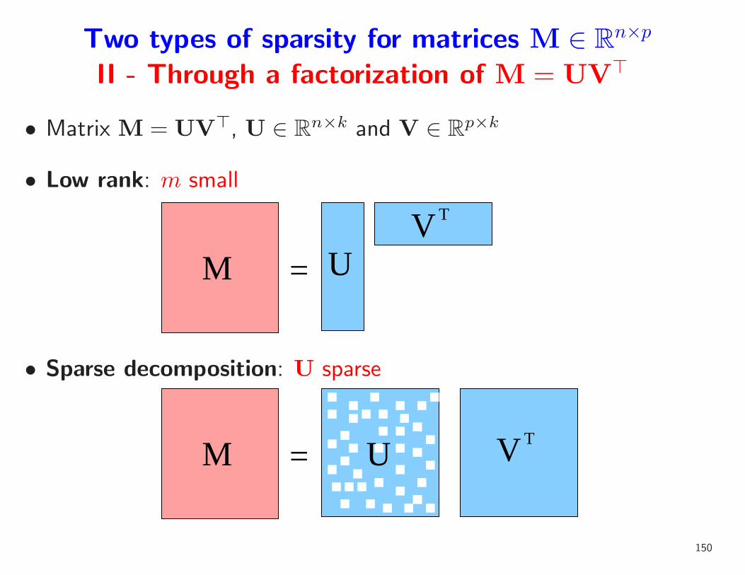
Two types of sparsity for matrices M ∈ Rn×p
II - Through a factorization of M = UV⊤
• Matrix M = UV⊤, U ∈ Rn×k and V ∈ R
p×k
• Low rank: m small
=
T
UV
M
• Sparse decomposition: U sparse
U= VMT
150

Structured sparse matrix factorizations
• Matrix M = UV⊤, U ∈ Rn×k and V ∈ R
p×k
• Structure on U and/or V
– Low-rank: U and V have few columns
– Dictionary learning / sparse PCA: U has many zeros
– Clustering (k-means): U ∈ 0, 1n×m, U1 = 1
– Pointwise positivity: non negative matrix factorization (NMF)
– Specific patterns of zeros (Jenatton et al., 2010)
– Low-rank + sparse (Candes et al., 2009)
– etc.
• Many applications
• Many open questions (Algorithms, identifiability, etc.)
151

Multi-task learning
• Joint matrix of predictors W = (w1, . . . , wk) ∈ Rp×k
• Joint variable selection (Obozinski et al., 2009)
– Penalize by the sum of the norms of rows of W (group Lasso)
– Select variables which are predictive for all tasks
152

Multi-task learning
• Joint matrix of predictors W = (w1, . . . , wk) ∈ Rp×k
• Joint variable selection (Obozinski et al., 2009)
– Penalize by the sum of the norms of rows of W (group Lasso)
– Select variables which are predictive for all tasks
• Joint feature selection (Pontil et al., 2007)
– Penalize by the trace-norm (see later)
– Construct linear features common to all tasks
• Theory: allows number of observations which is sublinear in the
number of tasks (Obozinski et al., 2008; Lounici et al., 2009)
• Practice: more interpretable models, slightly improved performance
153

Low-rank matrix factorizations
Trace norm
• Given a matrix M ∈ Rn×p
– Rank of M is the minimum size m of all factorizations of M into
M = UV⊤, U ∈ Rn×m and V ∈ R
p×m
– Singular value decomposition: M = UDiag(s)V⊤ where U and
V have orthonormal columns and s ∈ Rm+ are singular values
• Rank of M equal to the number of non-zero singular values
154

Low-rank matrix factorizations
Trace norm
• Given a matrix M ∈ Rn×p
– Rank of M is the minimum size m of all factorizations of M into
M = UV⊤, U ∈ Rn×m and V ∈ R
p×m
– Singular value decomposition: M = UDiag(s)V⊤ where U and
V have orthonormal columns and s ∈ Rm+ are singular values
• Rank of M equal to the number of non-zero singular values
• Trace-norm (a.k.a. nuclear norm) = sum of singular values
• Convex function, leads to a semi-definite program (Fazel et al., 2001)
• First used for collaborative filtering (Srebro et al., 2005)
155

Sparse principal component analysis
• Given data X = (x⊤1 , . . . ,x
⊤n ) ∈ R
p×n, two views of PCA:
– Analysis view: find the projection d ∈ Rp of maximum variance
(with deflation to obtain more components)
– Synthesis view: find the basis d1, . . . ,dk such that all xi have
low reconstruction error when decomposed on this basis
• For regular PCA, the two views are equivalent
156

Sparse principal component analysis
• Given data X = (x⊤1 , . . . ,x
⊤n ) ∈ R
p×n, two views of PCA:
– Analysis view: find the projection d ∈ Rp of maximum variance
(with deflation to obtain more components)
– Synthesis view: find the basis d1, . . . ,dk such that all xi have
low reconstruction error when decomposed on this basis
• For regular PCA, the two views are equivalent
• Sparse extensions
– Interpretability
– High-dimensional inference
– Two views are differents
∗ For analysis view, see d’Aspremont, Bach, and El Ghaoui (2008)
157

Sparse principal component analysis
Synthesis view
• Find d1, . . . ,dk ∈ Rp sparse so that
n∑
i=1
minαi∈Rm
∥∥∥∥xi −
k∑
j=1
(αi)jdj
∥∥∥∥
2
2
=n∑
i=1
minαi∈Rm
∥∥xi −Dαi
∥∥2
2is small
– Look forA = (α1, . . . ,αn) ∈ Rk×n and D = (d1, . . . ,dk) ∈ R
p×k
such that D is sparse and ‖X−DA‖2F is small
158

Sparse principal component analysis
Synthesis view
• Find d1, . . . ,dk ∈ Rp sparse so that
n∑
i=1
minαi∈Rm
∥∥∥∥xi −
k∑
j=1
(αi)jdj
∥∥∥∥
2
2
=n∑
i=1
minαi∈Rm
∥∥xi −Dαi
∥∥2
2is small
– Look forA = (α1, . . . ,αn) ∈ Rk×n and D = (d1, . . . ,dk) ∈ R
p×k
such that D is sparse and ‖X −DA‖2F is small
• Sparse formulation (Witten et al., 2009; Bach et al., 2008)
– Penalize/constrain dj by the ℓ1-norm for sparsity
– Penalize/constrain αi by the ℓ2-norm to avoid trivial solutions
minD,A
n∑
i=1
‖xi −Dαi‖22 + λk∑
j=1
‖dj‖1 s.t. ∀i, ‖αi‖2 6 1
159

Sparse PCA vs. dictionary learning
• Sparse PCA: xi ≈ Dαi, D sparse
160

Sparse PCA vs. dictionary learning
• Sparse PCA: xi ≈ Dαi, D sparse
• Dictionary learning: xi ≈ Dαi, αi sparse
161

Structured matrix factorizations (Bach et al., 2008)
minD,A
n∑
i=1
‖xi −Dαi‖22 + λk∑
j=1
‖dj‖⋆ s.t. ∀i, ‖αi‖• 6 1
minD,A
n∑
i=1
‖xi −Dαi‖22 + λn∑
i=1
‖αi‖• s.t. ∀j, ‖dj‖⋆ 6 1
• Optimization by alternating minimization (non-convex)
• αi decomposition coefficients (or “code”), dj dictionary elements
• Two related/equivalent problems:
– Sparse PCA = sparse dictionary (ℓ1-norm on dj)
– Dictionary learning = sparse decompositions (ℓ1-norm on αi)
(Olshausen and Field, 1997; Elad and Aharon, 2006; Lee et al.,
2007)
162

Dictionary learning for image denoising
x︸︷︷︸measurements
= y︸︷︷︸
original image
+ ε︸︷︷︸noise
163

Sparse methods for machine learning
Why use sparse methods?
• Sparsity as a proxy to interpretability
– Structured sparsity (Jenatton et al., 2009)
• Sparsity for high-dimensional inference
– Influence on feature design
• Sparse methods are not limited to least-squares regression
• Faster training/testing
• Better predictive performance?
– Problems are sparse if you look at them the right way
164

Conclusion - Interesting questions/issues
• Implicit vs. explicit features
– Can we algorithmically achieve log p = O(n) with explicit
unstructured features?
• Norm design
– What type of behavior may be obtained with sparsity-inducing
norms?
• Overfitting convexity
– Do we actually need convexity for matrix factorization problems?
165

Course outline
1. Losses for particular machine learning tasks
• Classification, regression, etc...
2. Regularization by Hilbertian norms (kernel methods)
• Kernels and representer theorem
• Convex duality, optimization and algorithms
• Kernel methods
• Kernel design
3. Regularization by sparsity-inducing norms
• ℓ1-norm regularization
• Multiple kernel learning
• Theoretical results
• Learning on matrices
166

Conclusion - Interesting problems
Machine learning for computer vision
• Kernel design for computer vision
– Benefits of “kernelizing” existing representations
– Combining kernels
• Sparsity and computer vision
– Going beyond image denoising
• Large numbers of classes
– Theoretical and algorithmic challenges
• Structured output
• Semi-supervised learning
167

References
Y. Amit, M. Fink, N. Srebro, and S. Ullman. Uncovering shared structures in multiclass classification.
In Proceedings of the 24th international conference on Machine Learning (ICML), 2007.
N. Aronszajn. Theory of reproducing kernels. Trans. Am. Math. Soc., 68:337–404, 1950.
F. Bach. Bolasso: model consistent lasso estimation through the bootstrap. In Proceedings of the
Twenty-fifth International Conference on Machine Learning (ICML), 2008a.
F. Bach. Exploring large feature spaces with hierarchical multiple kernel learning. In Adv. NIPS, 2008b.
F. Bach. Self-concordant analysis for logistic regression. Technical Report 0910.4627, ArXiv, 2009.
F. Bach, J. Mairal, and J. Ponce. Convex sparse matrix factorizations. Technical Report 0812.1869,
ArXiv, 2008.
F. R. Bach. Consistency of the group Lasso and multiple kernel learning. Journal of Machine Learning
Research, pages 1179–1225, 2008c.
F. R. Bach and M. I. Jordan. Kernel independent component analysis. Journal of Machine Learning
Research, 3:1–48, 2002.
F. R. Bach, G. R. G. Lanckriet, and M. I. Jordan. Multiple kernel learning, conic duality, and the SMO
algorithm. In Proceedings of the International Conference on Machine Learning (ICML), 2004a.
F. R. Bach, R. Thibaux, and M. I. Jordan. Computing regularization paths for learning multiple kernels.
In Advances in Neural Information Processing Systems 17, 2004b.
F. R. Bach, D. Heckerman, and E. Horvitz. Considering cost asymmetry in learning classifiers. Journal
of Machine Learning Research, 7:1713–1741, 2006.
168

O. Banerjee, L. El Ghaoui, and A. d’Aspremont. Model selection through sparse maximum likelihood
estimation for multivariate Gaussian or binary data. The Journal of Machine Learning Research, 9:
485–516, 2008.
A. Beck and M. Teboulle. A fast iterative shrinkage-thresholding algorithm for linear inverse problems.
SIAM Journal on Imaging Sciences, 2(1):183–202, 2009.
L. Benaroya, F. Bimbot, and R. Gribonval. Audio source separation with a single sensor. IEEE
Transactions on Speech and Audio Processing, 14(1):191, 2006.
D. Bertsekas. Nonlinear programming. Athena Scientific, 1995.
P. Bickel, Y. Ritov, and A. Tsybakov. Simultaneous analysis of Lasso and Dantzig selector. Annals of
Statistics, 37(4):1705–1732, 2009.
Karsten M. Borgwardt, Cheng Soon Ong, Stefan Schonauer, S. V. N. Vishwanathan, Alex J. Smola,
and Hans-Peter Kriegel. Protein function prediction via graph kernels. Bioinformatics, 21, 2005.
L. Bottou and C. J. Lin. Support vector machine solvers. In Large scale kernel machines, 2007.
Leon Bottou and Olivier Bousquet. Learning using large datasets. In Mining Massive DataSets for
Security, NATO ASI Workshop Series. IOS Press, Amsterdam, 2008. URL http://leon.bottou.
org/papers/bottou-bousquet-2008b. to appear.
E.J. Candes and Y. Plan. Near-ideal model selection by l1 minimization. The Annals of Statistics, 37
(5A):2145–2177, 2009.
E.J. Candes, X. Li, Y. Ma, and J. Wright. Robust principal component analysis? Arxiv preprint
arXiv:0912.3599, 2009.
Emmanuel Candes and Michael Wakin. An introduction to compressive sampling. IEEE Signal
169

Processing Magazine, 25(2):21–30, 2008.
O. Chapelle. Training a support vector machine in the primal. Neural Computation, 19(5):1155–1178,
2007.
Scott Shaobing Chen, David L. Donoho, and Michael A. Saunders. Atomic decomposition by basis
pursuit. SIAM Rev., 43(1):129–159, 2001. ISSN 0036-1445.
A. d’Aspremont, F. Bach, and L. El Ghaoui. Optimal solutions for sparse principal component analysis.
Journal of Machine Learning Research, 9:1269–1294, 2008.
D.L. Donoho and J. Tanner. Neighborliness of randomly projected simplices in high dimensions.
Proceedings of the National Academy of Sciences of the United States of America, 102(27):9452,
2005.
B. Efron, T. Hastie, I. Johnstone, and R. Tibshirani. Least angle regression. Ann. Stat., 32:407, 2004.
M. Elad and M. Aharon. Image denoising via sparse and redundant representations over learned
dictionaries. IEEE Trans. Image Proc., 15(12):3736–3745, 2006.
J. Fan and R. Li. Variable Selection Via Nonconcave Penalized Likelihood and Its Oracle Properties.
Journal of the American Statistical Association, 96(456):1348–1361, 2001.
M. Fazel, H. Hindi, and S.P. Boyd. A rank minimization heuristic with application to minimum
order system approximation. In Proceedings of the American Control Conference, volume 6, pages
4734–4739, 2001.
C. Fevotte, N. Bertin, and J.-L. Durrieu. Nonnegative matrix factorization with the itakura-saito
divergence. with application to music analysis. Neural Computation, 21(3), 2009.
S. Fine and K. Scheinberg. Efficient SVM training using low-rank kernel representations. Journal of
170

Machine Learning Research, 2:243–264, 2001.
P. A. Flach. The geometry of ROC space: understanding machine learning metrics through ROC
isometrics. In International Conference on Machine Learning (ICML), 2003.
W. Fu. Penalized regressions: the bridge vs. the Lasso. Journal of Computational and Graphical
Statistics, 7(3):397–416, 1998).
Thomas Gartner, Peter A. Flach, and Stefan Wrobel. On graph kernels: Hardness results and efficient
alternatives. In COLT, 2003.
K. Grauman and T. Darrell. The pyramid match kernel: Efficient learning with sets of features. J.
Mach. Learn. Res., 8:725–760, 2007. ISSN 1533-7928.
Z. Harchaoui and F. R. Bach. Image classification with segmentation graph kernels. In Proceedings of
the Conference on Computer Vision and Pattern Recognition (CVPR), 2007.
T. Hastie, R. Tibshirani, and J. Friedman. The Elements of Statistical Learning. Springer-Verlag,
2001.
T. Hastie, S. Rosset, R. Tibshirani, and J. Zhu. The entire regularization path for the support vector
machine. Journal of Machine Learning Research, 5:1391–1415, 2005.
T. J. Hastie and R. J. Tibshirani. Generalized Additive Models. Chapman & Hall, 1990.
David Haussler. Convolution kernels on discrete structures. Technical report, UCSC, 1999.
M. Hein and O. Bousquet. Hilbertian metrics and positive-definite kernels on probability measures. In
AISTATS, 2004.
R. Herbrich, T. Graepel, and K. Obermayer. Large margin rank boundaries for ordinal regression. In
Advances in Large Margin Classifiers. MIT Press, Cambridge, MA, 2000.
171

J. Huang, S. Ma, and C.H. Zhang. Adaptive Lasso for sparse high-dimensional regression models.
Statistica Sinica, 18:1603–1618, 2008.
R. Jenatton, J.Y. Audibert, and F. Bach. Structured variable selection with sparsity-inducing norms.
Technical report, arXiv:0904.3523, 2009.
R. Jenatton, J. Mairal, G. Obozinski, and F. Bach. Proximal methods for sparse hierarchical dictionary
learning. In Submitted to ICML, 2010.
T. Joachims. Making large-scale support vector machine learning practical. In Advances in kernel
methods — Support Vector learning. MIT Press, 1998.
T. Joachims. Optimizing search engines using clickthrough data. In ACM SIGKDD Conference on
Knowledge Discovery and Data Mining (KDD), pages 133–142, 2002.
Hisashi Kashima, Koji Tsuda, and Akihiro Inokuchi. Kernels for graphs. In Kernel Methods in
Computational Biology. MIT Press, 2004.
G. S. Kimeldorf and G. Wahba. Some results on Tchebycheffian spline functions. J. Math. Anal.
Applicat., 33:82–95, 1971.
G. R. G. Lanckriet, T. De Bie, N. Cristianini, M. I. Jordan, and W. S. Noble. A statistical framework
for genomic data fusion. Bioinf., 20:2626–2635, 2004a.
G. R. G. Lanckriet, N. Cristianini, L. El Ghaoui, P. Bartlett, and M. I. Jordan. Learning the kernel
matrix with semidefinite programming. Journal of Machine Learning Research, 5:27–72, 2004b.
S. Lazebnik, C. Schmid, and J. Ponce. Beyond bags of features: Spatial pyramid matching for
recognizing natural scene categories. In Proc. CVPR, 2006.
H. Lee, A. Battle, R. Raina, and A. Ng. Efficient sparse coding algorithms. In NIPS, 2007.
172

J. Liu, S. Ji, and J. Ye. Multi-Task Feature Learning Via Efficient l2,-Norm Minimization. Proceedings
of the 25th Conference on Uncertainty in Artificial Intelligence (UAI), 2009.
G. Loosli, S. Canu, S. Vishwanathan, A. Smola, and M. Chattopadhyay. Boıte a outils SVM simple et
rapide. Revue dIntelligence Artificielle, 19(4-5):741–767, 2005.
K. Lounici. Sup-norm convergence rate and sign concentration property of Lasso and Dantzig
estimators. Electronic Journal of Statistics, 2, 2008.
K. Lounici, A.B. Tsybakov, M. Pontil, and S.A. van de Geer. Taking advantage of sparsity in multi-task
learning. In Conference on Computational Learning Theory (COLT), 2009.
J. Lv and Y. Fan. A unified approach to model selection and sparse recovery using regularized least
squares. Annals of Statistics, 37(6A):3498–3528, 2009.
J. Mairal, F. Bach, J. Ponce, G. Sapiro, and A. Zisserman. Non-local sparse models for image
restoration. In International Conference on Computer Vision (ICCV), 2009.
H. M. Markowitz. The optimization of a quadratic function subject to linear constraints. Naval
Research Logistics Quarterly, 3:111–133, 1956.
N. Meinshausen. Relaxed Lasso. Computational Statistics and Data Analysis, 52(1):374–393, 2008.
N. Meinshausen and P. Buhlmann. High-dimensional graphs and variable selection with the lasso.
Annals of statistics, 34(3):1436, 2006.
N. Meinshausen and P. Buhlmann. Stability selection. Technical report, arXiv: 0809.2932, 2008.
N. Meinshausen and B. Yu. Lasso-type recovery of sparse representations for high-dimensional data.
Annals of Statistics, 37(1):246–270, 2008.
F. Meyer. Hierarchies of partitions and morphological segmentation. In Scale-Space and Morphology
173

in Computer Vision. Springer-Verlag, 2001.
Y. Nesterov. Introductory lectures on convex optimization: A basic course. Kluwer Academic Pub,
2003.
Y. Nesterov. Gradient methods for minimizing composite objective function. Center for Operations
Research and Econometrics (CORE), Catholic University of Louvain, Tech. Rep, 76, 2007.
G. Obozinski, M.J. Wainwright, and M.I. Jordan. High-dimensional union support recovery in
multivariate regression. In Advances in Neural Information Processing Systems (NIPS), 2008.
G. Obozinski, B. Taskar, and M.I. Jordan. Joint covariate selection and joint subspace selection for
multiple classification problems. Statistics and Computing, pages 1–22, 2009.
B. A. Olshausen and D. J. Field. Sparse coding with an overcomplete basis set: A strategy employed
by V1? Vision Research, 37:3311–3325, 1997.
J. Platt. Fast training of support vector machines using sequential minimal optimization. In Advances
in Kernel Methods: Support Vector Learning, 1998.
M. Pontil, A. Argyriou, and T. Evgeniou. Multi-task feature learning. In Advances in Neural Information
Processing Systems, 2007.
A. Rakotomamonjy, F. R. Bach, S. Canu, and Y. Grandvalet. Simplemkl. Journal of Machine Learning
Research, to appear, 2008.
Jan Ramon and Thomas Gartner. Expressivity versus efficiency of graph kernels. In First International
Workshop on Mining Graphs, Trees and Sequences, 2003.
P. Ravikumar, H. Liu, J. Lafferty, and L. Wasserman. SpAM: Sparse additive models. In Advances in
Neural Information Processing Systems (NIPS), 2008.
174

S. Rosset and J. Zhu. Piecewise linear regularized solution paths. Ann. Statist., 35(3):1012–1030,
2007.
V. Roth and B. Fischer. The group-Lasso for generalized linear models: uniqueness of solutions and
efficient algorithms. In Proceedings of the 25th International Conference on Machine Learning
(ICML), 2008.
B. Scholkopf and A. J. Smola. Learning with Kernels. MIT Press, 2001.
B. Scholkopf, J. C. Platt, J. S. Shawe-Taylor, A. J. Smola, and R. C. Williamson. Estimating the
support of a high-dimensional distribution. Neural Computation, 13(7):1443–1471, 2001.
S. Shalev-Shwartz, Y. Singer, and N. Srebro. Pegasos: Primal estimated sub-gradient solver for SVM.
In Proceedings of the International Conference on Machine Learning (ICML), 2007.
J. Shawe-Taylor and N. Cristianini. Kernel Methods for Pattern Analysis. Camb. U. P., 2004.
S. Sonnenburg, G. Rasch, C. Schafer, and B. Scholkopf. Large scale multiple kernel learning. Journal
of Machine Learning Research, 7:1531–1565, 2006.
N. Srebro, J. D. M. Rennie, and T. S. Jaakkola. Maximum-margin matrix factorization. In Advances
in Neural Information Processing Systems 17, 2005.
B. Taskar. Structured prediction: A large margin approach. In NIPS Tutorial, 2005. URL media.
nips.cc/Conferences/2007/Tutorials/Slides/taskar-NIPS-07-tutorial.ppt.
R. Tibshirani. Regression shrinkage and selection via the lasso. Journal of The Royal Statistical Society
Series B, 58(1):267–288, 1996.
S. A. Van De Geer. High-dimensional generalized linear models and the Lasso. Annals of Statistics, 36
(2):614, 2008.
175

R. Vert and J.-P. Vert. Consistency and convergence rates of one-class svms and related algorithms.
Journal of Machine Learning Research, 7:817–854, 2006.
S. V. N. Vishwanathan, A. J. Smola, and M. Murty. Simplesvm. In Proceedings of the International
Conference on Machine Learning (ICML), 2003.
G. Wahba. Spline Models for Observational Data. SIAM, 1990.
M. J. Wainwright. Sharp thresholds for noisy and high-dimensional recovery of sparsity using ℓ1-
constrained quadratic programming. Technical Report 709, Dpt. of Statistics, UC Berkeley, 2006.
L. Wasserman and K. Roeder. High dimensional variable selection. Annals of statistics, 37(5A):2178,
2009.
C. Watkins. Dynamic alignment kernels. Technical report, RHUL, 1999.
D.M. Witten, R. Tibshirani, and T. Hastie. A penalized matrix decomposition, with applications to
sparse principal components and canonical correlation analysis. Biostatistics, 10(3):515–534, 2009.
Tong Tong Wu and Kenneth Lange. Coordinate descent algorithms for lasso penalized regression. Ann.
Appl. Stat., 2(1):224–244, 2008.
M. Yuan and Y. Lin. Model selection and estimation in regression with grouped variables. Journal of
The Royal Statistical Society Series B, 68(1):49–67, 2006.
M. Yuan and Y. Lin. On the non-negative garrotte estimator. Journal of The Royal Statistical Society
Series B, 69(2):143–161, 2007.
T. Zhang. Adaptive forward-backward greedy algorithm for sparse learning with linear models. Advances
in Neural Information Processing Systems, 22, 2008a.
T. Zhang. Multi-stage convex relaxation for learning with sparse regularization. Advances in Neural
176

Information Processing Systems, 22, 2008b.
T. Zhang. On the consistency of feature selection using greedy least squares regression. The Journal
of Machine Learning Research, 10:555–568, 2009.
P. Zhao and B. Yu. On model selection consistency of Lasso. Journal of Machine Learning Research,
7:2541–2563, 2006.
H. Zou. The adaptive Lasso and its oracle properties. Journal of the American Statistical Association,
101(476):1418–1429, 2006.
H. Zou and R. Li. One-step sparse estimates in nonconcave penalized likelihood models. Annals of
Statistics, 36(4):1509–1533, 2008.
177