Open Journal of Statistics, 2016, 6, 842-861 http://www.scirp.org/journal/ojs

ISSN Online: 2161-7198 ISSN Print: 2161-718X

DOI: 10.4236/ojs.2016.65070 October 21, 2016

New Facts in Regression Estimation under Conditions of Multicollinearity

Anatoly Gordinsky

Berman Engineers LTD, Modiin, Israel

Abstract This paper considers the approaches and methods for reducing the influence of mul-ticollinearity. Great attention is paid to the question of using shrinkage estimators for this purpose. Two classes of regression models are investigated, the first of which corresponds to systems with a negative feedback, while the second class presents sys-tems without the feedback. In the first case the use of shrinkage estimators, especially the Principal Component estimator, is inappropriate but is possible in the second case with the right choice of the regularization parameter or of the number of prin-cipal components included in the regression model. This fact is substantiated by the study of the distribution of the random variable b b β β′ ′− , where b is the LS estimate and β is the true coefficient, since the form of this distribution is the basic charac-teristic of the specified classes. For this study, a regression approximation of the dis-tribution of the event 0b b β β′ ′− < based on the Edgeworth series was developed. Also, alternative approaches are examined to resolve the multicollinearity issue, in-cluding an application of the known Inequality Constrained Least Squares method and the Dual estimator method proposed by the author. It is shown that with a priori information the Euclidean distance between the estimates and the true coefficients can be significantly reduced.

Keywords Linear Regression, Multicollinearity, Two Classes of Regression Models, Shrinkage Estimators, Inequality Constrained Least Squres Estimator, Dual Estimator

1. Introduction

In the statistical literature, the term “multicollinearity” is almost as popular as the term “regression”. And this is natural since the regression analysis is one of the powerful tools to reveal dependencies which are hidden in the empirical data while multicolli-

How to cite this paper: Gordinsky, A. (2016) New Facts in Regression Estimation under Conditions of Multicollinearity. Open Journal of Statistics, 6, 842-861. http://dx.doi.org/10.4236/ojs.2016.65070 Received: August 10, 2016 Accepted: October 18, 2016 Published: October 21, 2016 Copyright © 2016 by author and Scientific Research Publishing Inc. This work is licensed under the Creative Commons Attribution International License (CC BY 4.0). http://creativecommons.org/licenses/by/4.0/

Open Access

A. Gordinsky

843

nearity is one of the main pitfalls of this approach. Indeed, a high correlation between two or more of the explanatory variables (predictors) sharply increases the variance of estimators, which adversely affects the study of a degree and a direction of the predictor action on the response variable. Multicollinearity also impairs the predictive opportuni-ties of the regression equation when the correlation in the new data significantly differs from the one in the training set. Numerous recent publications of researchers in various fields, such as medicine, ecology, economics, engineering, and others, devoted to the problem of multicollinearity, indicate that there are serious difficulties in this area until now. That is why the estimation of regression parameters under multicollinearity still remains one of the priorities of an applied and theoretical statistics.

The nature, methods of measurement, interpretation of the results, and methods of decreasing the effect of multicollinearity have been reviewed in numerous monographs and articles, of which we refer to the works have become classics [1]-[6] as well as the relatively recent articles [7]-[13].

In this paper, we focus on the parameters estimation methods in the multiple linear regression which corresponds to the following equation and assumptions

,Y X β= + (1)

where ( )2, , ~ 0,nY N σ∈ , 2σ is the variance of , ( ) 2cov nIσ= , known n kX ×∈ of rank k, and kβ ∈ is unknown.

Our goal is to consider the empirical and mathematical methods of improving the statistical characteristics of estimators and, consequently, facilitate their interpretation in conditions of multicollinearity. We also will briefly touch upon the questions of a prediction by regression equations.

Recommendations present in the literature to decrease the influence of multicolli-nearity, in particular in sources mentioned above, reduce to the following. 1) Eliminate the one of the predictors that is most strongly correlated with the others. 2) Ignore the multicollinearity issue if the regression model is designed for prediction. 3) Standardize the data. 4) Increase the data sample size. 5) Use the shrinkage, and therefore biased, estimators.

The approach formulated in the first item requires a careful analysis of the nature of the correlation between the predictors. In some cases, the deletion of some predic-tor can distort the essence of the regression model. For example, in studying a qua-dratic trend the linear term of an equation may be strongly correlated with the qua-dratic term, but the exclusion of one of them, of course, is unacceptable. Next will be considered a class of regression models for which such an exclusion is always unde-sirable.

The second approach is only acceptable when the correlation matrix of the new da-taset on which the prediction is being performed differs little from the same matrix of the training dataset. If this condition is not fulfilled, the variance of the prediction can increase many times. Unfortunately, experience in solving the real problems shows that the necessary proximity of the two indicated correlation matrices is rarely present.

A. Gordinsky

844

Data standardization undoubtedly improves the conditionality of computational al-gorithms for regression, which is essential with a high degree of multicollinearity. This effect is particularly useful in the case of polynomial regression models, and models containing certain other functions. According to the literature, the issue of the effect of standardization on the interpretability of the estimation results is still controversial and is not considered in this article.

Increasing the dataset size always improves the quality of the estimation. Unfortu-nately, in this case, the indicator of the severity of multicollinearity, called the variance inflation factor (VIF) [5], reduces proportionately to n , where n is the dataset size. This means, for example, that for an initial value of VIF = 50, one must increase n by a factor of 100 to reach the acceptable value VIF = 5. This is always expensive and is not always possible. Thus, given the above, it is advisable to study the last item of the rec-ommendations to reduce the impact of multicollinearity, namely, the use of shrinkage estimators.

We shall discuss further some features of the use of penalized estimators, which in-clude the ridge [14] and the Lasso [15] estimator, as well as the Principal Component estimator [16], and the James-Stein estimator [17]. The study of these estimators has been one of the key directions in statistics in recent decades. We show that there exists a class of regression models for which the application of the James-Stein estimator is useless, and employment of other mentioned estimators is dangerous. Moreover, this danger can be catastrophic for the PCR estimator. This statement is illustrated by the counterexample discussed in the second chapter. In the same chapter, on the basis of Monte Carlo trials, it is suggested that this situation is explained by the high probability of an event 0b b β β′ ′− < , where b is the LS estimator and β is the vector of the true regression coefficients.

This probability is studied in the third chapter. We obtained an analytical expression of the probability density function (pdf) for the simple regression, as well as analytical expressions for the four central moments for the multiple regression. Based on the last results, we derived an approximation of this pdf for multivariate regression, and its properties were examined.

The fourth chapter discusses the effect of the probability of the event 0st st st stb b β β′ ′− < on the efficiency of the shrinkage estimators. This study is based on numerical model-ing, the possibility of which is provided by the aforementioned approximation. The chapter introduces yet another class of regression models which is favorable for the ap-plication of shrinkage estimators. At the same time, the issue of setting the regulariza-tion parameter, which depends on the unknown coefficients β , remains open. In this case, the James-Stein estimator, which does not require a parameter of regularization, may provide only a meager improvement in efficiency.

Finally, the fifth chapter discusses alternative approaches. These approaches consist in an application of the known Inequality Constrained Least Squares method and the Dual estimator method proposed by the author in [18]. We show that in the presence of a priori information these approaches have significant advantages.

A. Gordinsky

845

2. Methods 2.1. Counter Example for Shrinkage Estimators: A Degree

of a Simultaneous Influence of Glucose and Insulin on the Blood Glucose Level

In this chapter, the author shows using counterexample that there are regression mod-els with a high degree of multicollinearity for which the use of shrinkage estimators are useless or nearly useless, in the best case, and in the worst case the first three of the above methods give the mean squares error ( MSE ) exceeding the quadratic risk 2L of the least square ( LS ) estimator. As far as the author knows, this fact was not consi-dered in the literature, although it may be very important for researchers.

Let us now suppose that a researcher has experimental data corresponding to the as-sumptions of the normal multivariate linear regression (1), and has found the Least Square estimate

( ) 1 .b X X X Y−′ ′= (2)

Let us also agree that the model is adequate, which means that F-criterion exceeds a critical value. This requirement is well founded as the estimate of coefficients does not make sense in the absence of adequacy. Moreover, the value of the F-test should exceed a critical value by several times [3], if one aims to ensure the acceptable quality of pre-diction with the regression model. This requirement for the value of the F-criterion would be more rigid, if one wishes to reach the sufficiently significance level of the es-timates of the regression coefficients. The further necessary condition is that the struc-ture of the regression model is found, and it does not change afterwards. Let there be multicollinearity existing in the experimental data. The researcher can apply four of the aforementioned shrinkage estimators to estimate the regression coefficients. The first three of them dominate only under certain conditions, whereas the fourth always do-minates, the LS estimator. The researcher, however, is not interested in domination it-self. Instead, he is interested in the quantitative characteristic of dominance, in particu-lar, the ratio of the mean squares error ( MSE ) to the quadratic risk 2L . As is known [6]

( ) ( ) ,shr shrMSE E b bβ β′= − − (3)

where shrb is shrinkage estimator, and

( )( )12 2 2

1,

k

ii

L Tr X Xσ σ λ−

=

′= = ∑ (4)

where Tr is the trace, iλ are the eigenvalues of the inverse matrix. The shrinkage estimator will be almost useless, if the ratio 2MSE L is insignifi-

cantly less than 1. Let us illustrate this assertion by the following example. Consider the problem of

computing of the maximum blood glucose in patients with the diabetes mellitus under the simultaneous action of the glucose given peroral, and the insulin given subcuta-neously. The physicians recommend [19] evaluating the influence of the insulin in order

A. Gordinsky

846

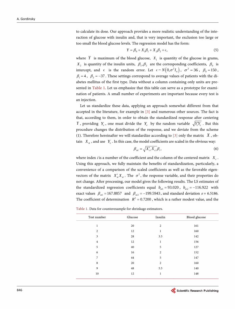
to calculate its dose. Our approach provides a more realistic understanding of the inte-raction of glucose with insulin and, that is very important, the exclusion too large or too small the blood glucose levels. The regression model has the form:

0 1 1 2 2 ,Y X Xβ β β= + ++ (5)

where Y is maximum of the blood glucose, 1X is quantity of the glucose in grams,

2X is quantity of the insulin units, 1 2,β β are the corresponding coefficients, 0β is intercept, and is the random error. Let ( )2~ 0, nN Iσ , 2 36σ = , 0 150β = ,

1 4β = , 2 37β = − . These settings correspond to average values of patients with the di-abetes mellitus of the first type. Data without a column containing only units are pre-sented in Table 1. Let us emphasize that this table can serve as a prototype for exami-nation of patients. A small number of experiments are important because every test is an injection.

Let us standardize these data, applying an approach somewhat different from that accepted in the literature, for example in [3] and numerous other sources. The fact is that, according to them, in order to obtain the standardized response after centering Y , providing cY , one must divide the cY by the random variable c cY Y′ . But this procedure changes the distribution of the response, and we deviate from the scheme (1). Therefore hereinafter we will standardize according to [3] only the matrix X , ob-tain stX , and use cY . In this case, the model coefficients are scaled in the obvious way:

,sti c i ci iX Xβ β′= (6)

where index i is a number of the coefficient and the column of the centered matrix cX . Using this approach, we fully maintain the benefits of standardization, particularly, a convenience of a comparison of the scaled coefficients as well as the favorable eigen-vectors of the matrix st stX X′ . The 2σ , the response variable, and their properties do not change. After processing, our model gives the following results. The LS estimates of the standardized regression coefficients equal 1 93.020stb = , 2 116.922stb = − with exact values 1 167.8857stβ = and 2 199.5943stβ = − , and standard deviation s = 6.5186. The coefficient of determination 2 0.7200R = , which is a rather modest value, and the

Table 1. Data for counterexample for shrinkage estimators.

Test number Glucose Insulin Blood glucose

1

2

3

4

5

6

7

8

9

10

20

12

28

12

40

16

44

20

48

12

2

1

3.5

1

5

2

5

2

5.5

1

161

160

142

156

127

152

147

160

140

148

A. Gordinsky

847

F-test at the significance level of 0.05 is equal to 8.99, which exceeds the critical value by a factor of 2.42. Finally, the t-tests respectively equal 1.898 and −2.386, while the critical value is 2.365 for the same significance level of 0.05. That is, we can see that the derived estimates of coefficients are almost not significant, despite the fact that the overall model is quite significant. The correlation matrix of the model is equal to

1.0000 0.99110.9911 1.0000

R =

, which indicates a high positive correlation of variables, variance

inflation factor (VIF) is 56 for both variables, so that the presence of the considerable multicollinearity is not in doubt. Now we have complete data which are necessary for further studies.

Let us evaluate the potential capabilities of the shrinkage estimators for our task. Consider first the ridge estimator [14] the original form of which for our technique of standardization is written as

( ) 1 ,r k st cb R rI X Y− ′= + (7)

where br is the ridge estimator, r > 0 is the regularization parameter, and we obtain the minimum MSE and the corresponding regularization parameter optr for (7).

For this we use approach [14] and derive the MSE expression in the matrix form:

( ) ( )21 2 2 ,st st n k st nMSE P I P Trβ β σ− −′ ′= Λ Λ − + Λ Λ (8)

where Λ is the diagonal matrix of the eigenvalues of the correlation matrix sorted in descending order, P is the matrix of the corresponding eigenvectors, n krIΛ = Λ + , and

kI is the identity matrix of order k. For our data, by minimizing stMSE and using (4) we find 58.85 10optr −= × , and 2 0.9901st stMSE L ≥ .

Thus in this task the ridge estimator is potentially useless. If we were to apply under the same conditions the technique of the automatic selec-

tion of r [3], wherein 2st str k b bσ ′= , we would derive by the Monte Carlo simulation

in MatLab that 2st stMSE L equals to 1.385.

As for the Lasso method, it is not possible to find the explicit expression for the

stMSE , and we again use the Monte Carlo approach in Matlab implementing the algo-rithm

{ }2

1arg min ,l LY Xββ β γ β= − + (9)

where lβ is the Lasso estimate, and 0γ > is constant of regularization, and compu-ting stMSE , 2

stL according to (3, 4) for big sets of and γ . The result is that 2 0.99st stMSE L > , i.e. this estimator is also potentially useless. It is also clear, if we es-

timate, using cross-validation as is customary [15], we find that the stMSE exceeds the 2stL . Here also note, that the exception of one of the predictors, which the Lasso may

accomplish, in our case will distort the substance of the model. Now we use the Monte Carlo method in an analogous manner to consider the possi-

bilities of Principal Component Regression (PCR) [16]. For this case we derive 2 16.4st stMSE L ≥ . This result should not be considered as too surprising, keeping in

A. Gordinsky

848

mind the precautions in the literature (see e.g. [6]) that excluding components corres-ponding to small eigenvalues may sharply reduce the quality of the estimation and pre-diction. In particular, in the brief review of opportunities of the shrinkage estimators made in [18] this fact is confirmed by an analysis of the simulation outcomes in [20].

Finally, as to the James-Stein estimator, in our problem, we cannot apply this method in a canonical form [17], as the number of predictor variables is less than three. But nothing prevents us from deriving the stMSE for the general kind of the shrinkage es-timator that is employed in the James-Stein approach, exactly:

,shrb bψ= (10)

where 0ψ > is some constant. Under known ψ and stβ after obvious calculations we obtain

( )22 2 1 ,optst st opt st stMSE Lψ ψ β β′≥ + − (11)

where

( )( )( )12 .opt st st st st st sttrace X Xψ β β β β σ −′ ′ ′= + (12)

For our data we have 2 0.944st stMSE L ≥ . Thus there are models with a high degree of multicollinearity for which the applica-

tion of the shrinkage estimators is at least virtually useless. What is the reason for this phenomenon?

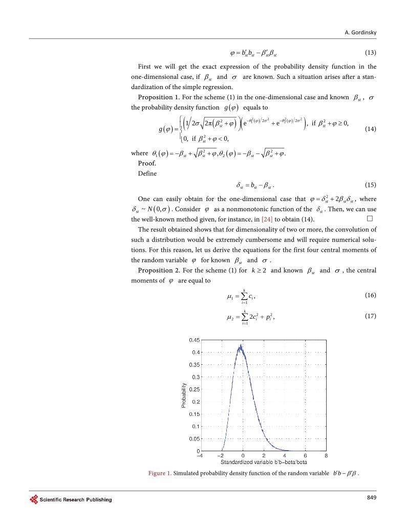
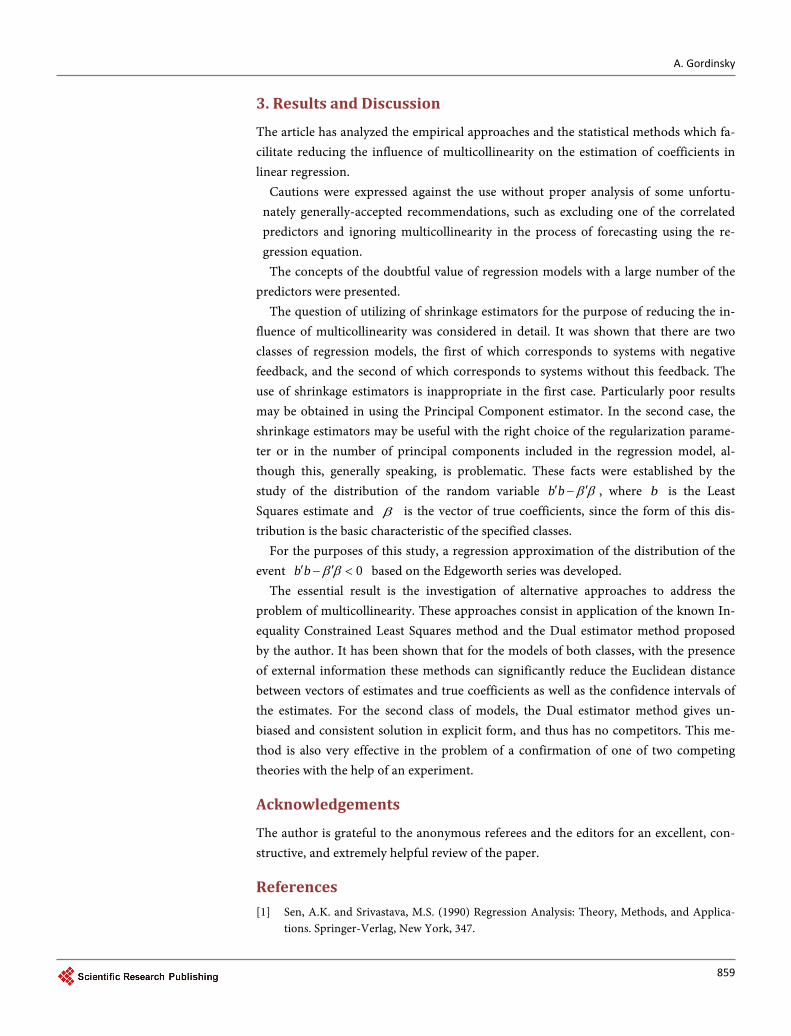
To answer this question, let us simulate the density of the random variable

st st st stb b β β′ ′− by the Monte Carlo method. The probability density function based on implementations of 106 tests is shown in Figure 1.

For the approximation presented, we obtained: ( )Pr 0 0.4996st st st stb b β β′ ′− < = , where Pr is probability. It was namely this fact which provides the answer to our question. It turns out that, contrary to established beliefs, significant multicollinearity does not always lead to an increase in the average norm of LS-estimates regarding the norm of the true coefficients. There are situations possible in which this norm is almost equal to the norm of the true coefficients. This results in an increase of the component MSE caused by the bias and a reduction of effectiveness of shrinkage estimators, which is precisely what we have observed.

It is evident that in order to ascertain the reasons for such a situation, it is necessary to explore the properties of the distribution of the random variable st st st stb b β β′ ′− , which is the purpose of the next chapter.

2.2. Properties of the Distribution of the Random Variable ′ ′st st st stb b − β β

In this chapter, it will be shown that the random variable under study can be represented as a sum of the independent weighted central chi-square and normal va-riables. The author could not find the explorations of the distribution for this case, de-spite a vast literature on an approximation of the distribution of a sum of weighted chi-square variables (e.g., [21]-[23]). Let us define

A. Gordinsky

849

st st st stb bϕ β β′ ′= − (13)

First we will get the exact expression of the probability density function in the one-dimensional case, if stβ and σ are known. Such a situation arises after a stan-dardization of the simple regression.

Proposition 1. For the scheme (1) in the one-dimensional case and known stβ , σ the probability density function ( )g ϕ equals to

( ) ( )( ( ) ( )( )2 2 2 21 22 22 2

2

1 2 2π e e , if 0,

0, if 0,

st st

st

gθ ϕ σ θ ϕ σσ β ϕ β ϕ

ϕβ ϕ

− − + + + ≥ = + <

(14)

where ( ) ( )2 21 2, .st st st stθ ϕ β β ϕ θ ϕ β β ϕ= − + + = − − +

Proof. Define

st st stbδ β= − . (15)

One can easily obtain for the one-dimensional case that 2 2st st stϕ δ β δ= + , where ( )~ 0,st Nδ σ . Consider ϕ as a nonmonotonic function of the stδ . Then, we can use

the well-known method given, for instance, in [24] to obtain (14). The result obtained shows that for dimensionality of two or more, the convolution of

such a distribution would be extremely cumbersome and will require numerical solu-tions. For this reason, let us derive the equations for the first four central moments of the random variable ϕ for known stβ and σ .

Proposition 2. For the scheme (1) for 2k ≥ and known stβ and σ , the central moments of ϕ are equal to

11

,k

ii

cµ=

= ∑ (16)

2 22

12 ,

k

i ii

c pµ=

= +∑ (17)

Figure 1. Simulated probability density function of the random variable b b β β′ ′− .

A. Gordinsky

850

3 23

18 6 ,

k

i i ii

c c pµ=

= +∑ (18)

4 2 2 44 2 2

160 60 3 6 ,

k

i i i i i ji i j

c c p pµ µ µ= <

= + + +∑ ∑ (19)

2 ,i ic σ λ= (20)

2 ,i st i ip zβ σ λ′= (21)

where iλ is the eigenvalue of inverse of the correlation matrix 1R− , and iz is the corresponding eigenvector of the same matrix.

Proof. In the multidimensional case using (13), (15) we derive

2st st st stϕ δ δ β δ′ ′= − . (22)

Taking into account the orthogonality of the eigenvectors we represent ϕ as fol-lows: 2st st st stzz zzϕ δ δ β δ′ ′ ′ ′= − . Examining the vector stz δ′ , we derive the result that its components have normal distribution with zero expectation and variance of 2

iσ λ . Furthermore, these components are noncorrelated due to orthogonality of the eigen-vectors and hence are independent together with functions of them. Therefore, using the notation (20), (21) we find:

2

1,

k

i i i ii

c pϕ α α=

= +∑ (23)

where ( )0,1i Nα and ( ) 2cov kIα σ= . We find the moments about the origin of one of the independent variables 2

i i i ic pα α+ taking for k = 1 - 4 the definite integrals

( ) 22 21 e d2π

kx

i ic x p x x∞ −

−∞+∫ . Then we find the central moments, using the known re-

lation for their calculations ( ) 10

1n n j n j

n jj

nM M

jµ − −

=

= −

∑ , where µ and M are the

central and the initial moments. It remains to find the central moments for the sums of the independent random variables, which is performed according to the well-known rules.

Once these moments are found, one can, if necessary, approximate the distribution by well-known methods using Pearson’s or Johnson’s families of curves [25] or by ex-pansion into a certain series [26]. However, our ultimate goal is to estimate the proba-bility of fulfillment of the inequality 0st st st stb b β β′ ′− < , since it is specifically this which has a decisive influence on the expedience of the application of shrinkage estimators. Therefore let us simplify the task, and we will approximate this probability

( )Pr 0st st st stb b β β′ ′− < . For the approximation we use variables that are included in the Edgeworth’s series [25] [27] and we construct the regression on these variables. This approach is used because direct application of the specified series for our distribution does not provide an acceptable accuracy.

Let us designate

1 2 ,x µ µ= (24)

A. Gordinsky

851

( ) 2 21 2π e ,xq −= (25)

( )( )0.5 1 2 ,P erf x= − (26)

( )23 1 ,P x q= − (27)

( )5 36 10 15 ,P x x x q= − − + (28)

( )8 6 4 29 28 210 420 105 ,P x x x x q= − + − + (29)

as well as the skewness, the kurtosis, and the relative fifth central moment 1.5

3 2 ,kS µ µ= (30)

24 2 ,Ku µ µ= (31)

2.55 5 2 .Ku µ µ= (32)

Note that the indexes in (27-29) are equal to the indexes of the corresponding Her-mite polynomials. The vector-row U of the first seven variables included in the Edge-worth series appears as follows

( ) ( ) ( )2 35 54 73 6 9103 3

6 24 72 120 144 1296k kk k kKu S PKu P S Ku PS P S P S PU P

− −− − −= − − .

By using the probabilistic genetic algorithm, a model with interaction term is ob-taining including the next four variables: intercept, ( ) ( ) ( ) ( )1 , 2 , 4 7U U U U . After transformation, model for the estimator r̂P of the probability of the event

0st st st stb b β β′ ′− < has the form:

( ) ( ) ( ) ( )( )43 6 9

ˆ 1 2 3 4 ,r k kP a a P a S P a S P P= + + + (33)

where ( )a i is the corresponding element of the vector-row of coefficients a : 30.0498380531724143 1.11882644043104 0.17343711278363 0.167210843039776 10 .a − = − − ×

In addition, if ˆ 0rP < , we take ˆ 0rP = , if ˆ 0.5rP > , we take ˆ 0.5rP = . The above coefficients were established as follows. 15 tasks were generated and taken

from literature, while for each of which 100 variants of the coefficients were used. That is, the volume of the training set was 1500. In the process we kept in mind the above mentioned restrictions to the coefficient of determination 2R , and the value of σ was selected accordingly. The true probability of fulfilment of the above mentioned in-equality was calculated using a Monte Carlo method with a number of tests equals

62 10× . The number of the predictors ranged from two to ten. The maximum number of predictors taken requires some explanation. The literature

data and the author’s experience shows that the number of predictors permitting one to reach values of the coefficient of determination R2 of 0.8 and above, with rare excep-tions does not exceed ten, if the researcher properly use the methodology of the model selection as well as the nonlinear predictors (in particular, the multivariate polyno-mials). It seems reasonable to argue that the steadily functioning technical, biological or

A. Gordinsky

852

other systems cannot be stable under a large number of degrees of freedom. As exam-ples for such arguments, let us refer to the following works [28]-[33].

In all these works, despite the heterogeneity of the modeling objects, the number of variables in the model does not exceed nine, with variations of 2R within the range 0.74 - 0.99. A rather characteristic situation has arisen during the research considered in [29]. The discussion in the journal Chemical Fibres in the former USSR, with the in-volvement of the leading theorists and practitioners, has identified 150 factors influen-cing the structure of the viscose fibres. At the same time the parametrically linear re-gression model of the indicator of the structure uniformity contained eight polynomial variables and had 2 0.85R = . The last value proved to be the maximum achievable for the characteristics of the measurement errors in the experiment. A good confirmation of the efficiency of this model was the fact that a change of the parameters of the fabri-cation process carried out on the basis of the model equation provided very high in-crease of the highest-quality product. Note also, when constructing the model of the probability presented above (33), there was a set of 35 possible multivariate polyno-mials of the second order. However, only three variables entered the model, providing

2 0.985R = . Let us consider the validation of the received model (33). Similar to the formation of

the training set, the testing set of the same size was created. For this set, the following characteristics of the errors in the calculation of the probability are obtained: mean value −0.00054 against 0.00022 in the training set, the standard deviation 0.01289 against 0.01598, skewness 0.64 and kurtosis 9.17. 95 percent of the errors lie in the in-terval [−0.024583 0.028161]. We add that Equation (33) has also been continuously tested in the subsequent investigations and corresponded to the above results. Thus one can consider that the model (33) provides acceptable accuracy in determining the probability of the event 0st st st stb b β β′ ′− < . Note, incidentally, that the error in the de-termination of the probability in the problem discussed in the introduction, is 0.00468.

Let us give some properties of the probability under study. 1) As can be seen from (16-21) the central moments are even functions of zβ ′ . Thus

the probability is also an even function. In other words, a simultaneous change of all signs of the coefficients does not change the probability.

2) For fixed values of the coefficient of determination 2R the product zβ ′ has the decisive influence on the probability. We illustrate this assertion by an example on the data [5] (table D11, Example of multicollinearity). The average VIF for them equals 459, so there is a very high degree of multicollinearity. Let us set the values of the coef-

ficients as follows: 3.01.71.2

β = − −

(then standardized coefficients are equal to

65.6938.7919.08

stβ −−

=

). Next, let us add to the response the normal noise providing 2 0.85R = .

The probability of the event 0st st st stb b β β′ ′− < calculated from (33) equals 0.462. Now

A. Gordinsky

853

we change the sign of the first coefficient to its opposite and add the normal noise with the different variance, so that 2R remains the same. The Equation (33) gives a proba-bility of 0.09.

Thus, under equal values of 2R and st stβ β′ but different signs of the coefficients and therefore the other value of the product zβ ′ , the probability can be drastically dif-ferent.

3) For any sample available to the researcher, even in the presence of a high degree of multicollinearity, the probability of the event 0st st st stb b β β′ ′− < can range from 0 to 0.5. This probability depends on the coefficients β , their signs, and the properties of the matrix X, specifically its eigenvalues and eigenvectors. The value of the σ , from which the distribution under study depends, can be easily calculated, if ,X Y , and β are known. However, since in real life the coefficients β and their signs are un-known, it is not possible to evaluate the probability without a priori information. The attempt to use the LS estimates derived from a sample can be misleading because the latter can sharply differ from the true coefficients by the magnitudes and signs.

4) The probability increases with the increase in the coefficient of determination 2R , if the magnitudes and signs of the true coefficients are unchanged. Having derived the above results, in the next section the author will try to assess how

the magnitude of the investigated probability affects the efficiency of the shrinkage es-timators.

2.3. The Influence of the Probability Magnitude of the Event ′ ′st st st stb b − < 0β β on the Efficiency of the Shrinkage Estimators

In this chapter, the following shrinkage estimators will be considered: ridge estimator, the principal component estimator, and the James-Stein estimator. The Lasso method will not be considered separately, because this approach yields result that is close to the result of the ridge estimator, if the structure of the model is unchanged, as it was adopted in this paper. To calculate the above estimators we use the algorithms pre-sented in [34]. Modeling of a number of tasks under the above stipulated conditions leads to the following conclusions.

1) The case of high probability of the considered event (0.4 and more). First, note that in this case about half of the shrinkage point estimates will be worse

than the LS point wise estimates. Further, the high probability unconditionally nega-tively affects the MSE of the shrinkage estimators. In this case, for the James-Stein es-timator the ratio 2

st stMSE L is very close to 1. In addition, this estimator cannot cor-rect the false signs of the coefficients obtained by the LS method. The risk of the ridge regression is slightly less than the risk of the LS estimator or exceeds it, if we choose the regularization parameter in (7) as 2r ks b b′= [14]. In the latter case, the ratio

2st stMSE L can reach a value of 1.65. The Principal Component estimator may re-

spond to a high probability dramatically. Recall, in the example discussed in the intro-duction 2 16.4st stMSE L = , while in the example of the second paragraph of the pre-vious chapter this ratio is 5.5. In the generated example with 10 variables, sample size

A. Gordinsky

854

70, and average VIF equal to 123, the ratio 2st stMSE L fluctuates in a small range

around the value of 119 when we change the number of components from 1 to 9. It should be added that in the present case, the PCR estimator often gives such small ab-solute values of the coefficients that researcher may conclude that the predictors in-cluded in the model, do not in any way affect the response. But this may absolutely not correspond to reality. In addition, greater differences were observed in the value of

2st stMSE L when preserving a different number of components.

2) The case of low probability of the considered event (0.3 and less). This case is more favorable for the use of shrinkage estimators. So, for the James-

Stein estimator we successfully reached 2 0.87st stMSE L = , for the F criterion and 2R in the range given above. The ridge estimator provides a significant reduction in the ra-tio 2

st stMSE L which can reach a value of 0.4 or even less. The Principal Component estimator gives the similar results. In both cases however, despite the decrease in this ratio the risk may be unsatisfactory for practical application for a high degree of multi-collinearity. As a result one should increase the 2R and thus increase the probability, which can reach high values. It is important to emphasize the following. Paradoxically as it may seem, the risk of the LS estimator and simultaneously the risk of the shrinkage estimators for small probabilities may be considerably larger than under large probabil-ities even though the 2R and the sum of squares of the true coefficients β are the same.

So, we found that the probability of the event 0st st st stb b β β′ ′− < significantly affects the efficiency of the shrinkage estimators, especially the PCR estimator. But the re-searcher cannot assess this probability, since it depends on the unknown parameters β . Therefore, a reasonable way is to use a priori information. Apparently, the first thing to take into account is the following.

The analysis shows that a high probability of the event 0st st st stb b β β′ ′− < occurs when the regression model describes a system in which there is a compensation of the influence of some factor by other factor. In the language of control theory this is called negative feedback. The example discussed in the introduction illustrates such a situa-tion: the insulin compensates the glucose effect. If the researcher knows a priori that such compensation exists, then using shrinkage estimators is inexpedient.

Low probability of the event 0st st st stb b β β′ ′− < corresponds to a different class of re-gression models in which there is multicollinearity but there is no compensation. An example of the such opposite situation is when the regression model establishes a rela-tionship between the temperature at some point of the steam turbine path and two oth-er temperatures ahead of this place [28]. Generally, last two temperatures significantly correlated, that is, multicollinearity is there exists, but compensation in the above sense is absent. In this case, there is reason to assume that the shrinkage estimators is appro-priate. However, the difficulties of choosing the regularization parameter or amount of stored components remain. As for the James-Stein estimator, the benefit is small as shown above. Furthermore, as shown in [18], efficiency of this estimator decreases with increasing 2R .

A. Gordinsky

855

2.4. The Inequality Constrained Least Squares and the Dual Estimator Methods in Conditions of Multicollinearity

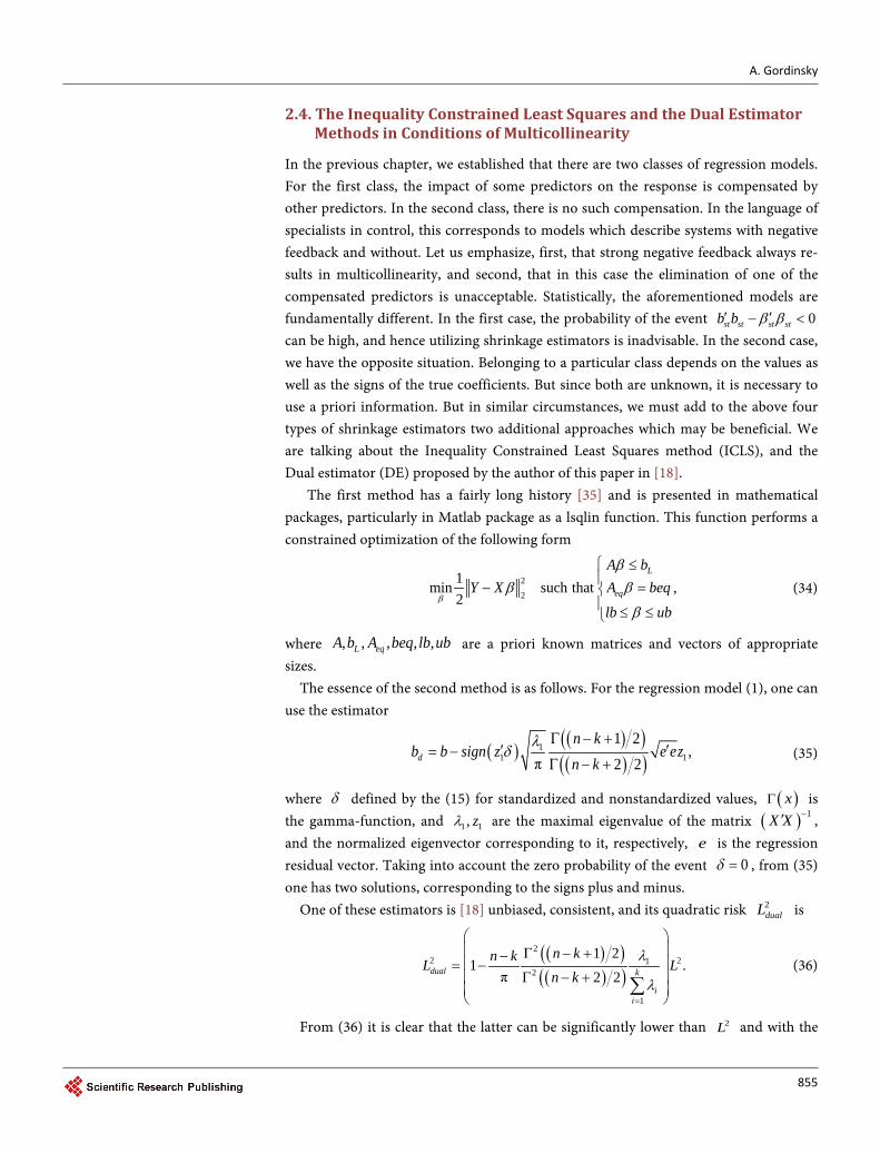
In the previous chapter, we established that there are two classes of regression models. For the first class, the impact of some predictors on the response is compensated by other predictors. In the second class, there is no such compensation. In the language of specialists in control, this corresponds to models which describe systems with negative feedback and without. Let us emphasize, first, that strong negative feedback always re-sults in multicollinearity, and second, that in this case the elimination of one of the compensated predictors is unacceptable. Statistically, the aforementioned models are fundamentally different. In the first case, the probability of the event 0st st st stb b β β′ ′− < can be high, and hence utilizing shrinkage estimators is inadvisable. In the second case, we have the opposite situation. Belonging to a particular class depends on the values as well as the signs of the true coefficients. But since both are unknown, it is necessary to use a priori information. But in similar circumstances, we must add to the above four types of shrinkage estimators two additional approaches which may be beneficial. We are talking about the Inequality Constrained Least Squares method (ICLS), and the Dual estimator (DE) proposed by the author of this paper in [18].

The first method has a fairly long history [35] and is presented in mathematical packages, particularly in Matlab package as a lsqlin function. This function performs a constrained optimization of the following form

2

2

1min such that ,2

L

eq

A bY X A beq

lb ubβ

ββ β

β

≤− = ≤ ≤

(34)

where , , , , ,L eqA b A beq lb ub are a priori known matrices and vectors of appropriate sizes.

The essence of the second method is as follows. For the regression model (1), one can use the estimator

( )( )( )( )( )

11 1

1 2,

π 2 2d

n kb b sign z e ez

n kλ

δΓ − +

′ ′= −Γ − +

(35)

where δ defined by the (15) for standardized and nonstandardized values, ( )xΓ is the gamma-function, and 1 1, zλ are the maximal eigenvalue of the matrix ( ) 1X X −′ , and the normalized eigenvector corresponding to it, respectively, e is the regression residual vector. Taking into account the zero probability of the event 0δ = , from (35) one has two solutions, corresponding to the signs plus and minus.

One of these estimators is [18] unbiased, consistent, and its quadratic risk 2dualL is

( )( )( )( )

222 1

2

1

1 21

π 2 2.dual k

ii

n kn kLn k

Lλ

λ=

Γ − +−−

Γ − +

=

∑ (36)

From (36) it is clear that the latter can be significantly lower than 2L and with the

A. Gordinsky

856

growth of a degree of multicollinearity the effectiveness of the Dual estimator increases

with the ratio 1

1

k

iiλλ

=∑ other factors being equal. Choosing the right solutions of the

two alternatives (35) is carried out through the use of a priori information. It is also important that the method allows estimating of only part of the coefficients naturally for predictors that highly correlated with the others.

The value of any method of estimation based on the use of a priori information largely defined by its universality regarding possible forms of this information.

The shrinkage estimators allow only one kind of a priori information, which confirms the validity of the inequality b b β β′ ′> and do not admit the nonstrict inequalities.

The Inequality Constrained Least Squares method has a high degree of flexibility, as is evident from (34) allowing to take into account constraints on the unknown regres-sion coefficients in the form of systems of inequalities and equalities simultaneously. However, unlike the shrinkage estimators, this method permits only nonstrict inequali-ties, for example lb ubβ≤ ≤ . Therefore, inequalities of the type i jβ β> cannot be utilized. In addition, if the some element of the vector lb or ub equal to zero, due to the nature of the optimization algorithm one can obtain the estimate 0iβ = , which is often meaningless. A significant drawback is the fact that, if a priori information is re-lated to the response, the researcher need to solve the inverse problem in order to ob-tain the inequalities for the regression coefficients. And it can be very difficult.

The possibility of using a priori information for the Dual estimator is entirely uni-versal. The advantages of this method are most obvious in the two following situations. The first of these, which is considered in the previous chapter as an example of the re-gression model for temperatures, is characterized by the presence multicollinearity and an absence of mutual compensation of the influence of the predictors. In this case, In-equality Constrained Least Squares method is not applicable, the shrinkage estimators are biased and require the additional parameters, whereas the Dual estimator method gives the unbiased and consistent solution in the explicit form

( )( )( )( )( )

11 1

1 2π 2 2

.d

n kb b sign z b e ez

n kλ Γ − +

′ ′= −Γ − +

(37)

As indicated, the example of the first situation given in the previous section is the dependence of some temperature on two others. If we use the method under study and (4), (33), (36), we obtain the probability 0.266rP = and 2 2

_ 0.376dual st stL L = , which is completely satisfactory. We point out that for this estimator there remains in force the above precaution with regard to the increase of the risk under the low probability.

Note also, that a priori information considered is qualitative, and thus in many cases it is the least burdensome and, hence, convenient for the researcher.

The second situation consists in confirmation of one of two competing theories with the help of an experiment. Application of the Dual estimator in this case is illustrated in details by a verification of the General Theory of Relativity based upon astronomical data [18].

Of interest are the possibilities of the methods considered for solving the problem

A. Gordinsky

857

presented in the first chapter as a counterexample. Suppose the researcher have a priori information regarding the coefficient at a dose of insulin, which consists in the fact that

245 25β− ≤ ≤ − . For the standardized coefficient, one can obtain 2242.7 134.8stβ− ≤ ≤ − .

Let us use this information and find the ICLS estimate. In our case 242.7

lb−∞

= − ,

134.8ub

∞ = −

. The lsqlin function gives the solution 110.74

134.8iclsb = −

. Obviously, this

solution is closer to the true values 167.89199.59stβ

= −

than the LS estimate

93.02116.92stb

= − . Let us now find the Dual estimate. Calculating the standardized values

1 2,st stb b we derive using (35) 1

128.4152.28stb

= − , 2

57.6481.57stb

= − . It is evident that 2stb

does not correspond to a priori information, and our solution will be 1stb . This solu-tion is better than the previous one provided by lsqlin. We add that the length of indi-vidual confidence intervals, which is calculated by the expression (43) presented below, equals 0.636 times the same intervals for the LS estimate.

Let us now compare the capabilities of the two methods under study on a set of trials of the first, difficult for estimation, class of regression models with a constraint in the form of nonstrict inequality. For the Dual estimator method, we shall apply the follow-ing algorithm to account for a priori information.

Let the limits for some true regression coefficient 1 2ia aβ≤ ≤ be known to the re-searcher. At this point, the reader may wonder why we are considering restrictions only for one coefficient. Our answer is that this is the most available constraint in many ap-plications, since if we have a system of the inequalities for several coefficients then an intractable question of its consistency arises. In addition, under conditions of multicol-linearity, when one coefficient is known the others are well established using Equation (41), presented below.

Let us find the estimate d ib for the coefficient iβ by the following rule

1 2

1 1

2 2

1 1

2 2

, if, if, if ,

, if, if

i i

i i

d i i i

i

i

b a b ab p a p b a

b b p a b a pa b a pa b a p

≤ ≤ + − < <= − < < + < − > +

(38)

where

( )( )( )( )

, 1 2 ,

π 2 2i ip

n kGe e

n kΓ − +

′=Γ − +

(39)

and ,i iG is a diagonal element with the number i of the inverse matrix G:

( ) 1 .G X X −′= (40)

Having found d ib we can obtain the remaining coefficients using the known expres-

A. Gordinsky

858

sion for the LS estimator with restrictions in the form of equation [3]:

( ) ( )( ) ( )11 1 ,d d ib b X X H H X X H b Hb−− −′ ′ ′ ′= + − (41)

in which H is a row vector of size k that contains 1 in the ith position and zeroes in all the remaining positions.

Let us illustrate this method on the counterexample from the second Chapter. Using Monte Carlo method let us compute Euclidean distances between the estimates and the true values of the coefficients for the two methods (ICLS and DE) and then we find the ratio of these distances to the same distance, given by the LS method. We obtain the ra-tio of 0.67 for the rule (38)-(41) and 0.78 for the Inequality Constrained Least Squares method. While extremely unsymmetrical a priori interval will give these ratios 0.70 and 0.71 respectively.

These results are consistent with the detailed research in [18]. For the first method, a priori information which is symmetric with respect to the parameter iβ gives on 15 - 20 percent less distance. For extremely asymmetric information distances are almost equal. i.e. an average the first method has an advantage.

Finally, consider the question relative to the individual confidence intervals in the Dual estimator. Let 1db be the estimator which corresponds to the plus sign in (35) and 2db be estimator which corresponds to the minus sign. As values 1a and 2a are known let us find d ib from (38) and the closest to this estimate ith element of the three possible vectors 1 2, ,i d i d ib b b .

The initial individual confidence intervals for these three values are [3] [18]:

( ) ( ) 1,,1 2 ,ii iXb t k sXn α −± − − ′ (42)

( )1 ,,1 2 ,d i iib n k sQt α± − − (43)

( )2 ,,1 2 ,d i iib n k sQt α± − − (44)

( ) ( )( )( )( )( )

21 1

1 12

1 2,

π 2 2n k

Q X X n k z zn k

λ− Γ − +′ ′= − −

Γ − + (45)

where ( ),1 2t n k α− − is the 1 2α− point of the Student distribution with n k− degrees of freedom, ,i iQ is the corresponding diagonal element of the matrix Q from (45).

It remains to find the intersection of the confidence interval specified for the nearest element and a priori interval. This intersection will be the new confidence interval. The confidence intervals for the remaining coefficients are easily found with the aid of equ-ation (41).

It is clear that one should compare the width of the new confidence intervals with the width of a priori interval. It is likewise evident that new confidence intervals cannot be wider than a priori intervals. Their ratio depends on the data sample properties, the value of a priori interval, and its location relative to the sought parameter. Tests on a large number of independent tasks have shown that a new confidence interval may be less by a factor of 1.3 than the a priori interval.

A. Gordinsky

859

3. Results and Discussion

The article has analyzed the empirical approaches and the statistical methods which fa-cilitate reducing the influence of multicollinearity on the estimation of coefficients in linear regression.

Cautions were expressed against the use without proper analysis of some unfortu-nately generally-accepted recommendations, such as excluding one of the correlated predictors and ignoring multicollinearity in the process of forecasting using the re-gression equation.

The concepts of the doubtful value of regression models with a large number of the predictors were presented.

The question of utilizing of shrinkage estimators for the purpose of reducing the in-fluence of multicollinearity was considered in detail. It was shown that there are two classes of regression models, the first of which corresponds to systems with negative feedback, and the second of which corresponds to systems without this feedback. The use of shrinkage estimators is inappropriate in the first case. Particularly poor results may be obtained in using the Principal Component estimator. In the second case, the shrinkage estimators may be useful with the right choice of the regularization parame-ter or in the number of principal components included in the regression model, al-though this, generally speaking, is problematic. These facts were established by the study of the distribution of the random variable b b β β′ ′− , where b is the Least Squares estimate and β is the vector of true coefficients, since the form of this dis-tribution is the basic characteristic of the specified classes.

For the purposes of this study, a regression approximation of the distribution of the event 0b b β β′ ′− < based on the Edgeworth series was developed.

The essential result is the investigation of alternative approaches to address the problem of multicollinearity. These approaches consist in application of the known In-equality Constrained Least Squares method and the Dual estimator method proposed by the author. It has been shown that for the models of both classes, with the presence of external information these methods can significantly reduce the Euclidean distance between vectors of estimates and true coefficients as well as the confidence intervals of the estimates. For the second class of models, the Dual estimator method gives un-biased and consistent solution in explicit form, and thus has no competitors. This me-thod is also very effective in the problem of a confirmation of one of two competing theories with the help of an experiment.

Acknowledgements

The author is grateful to the anonymous referees and the editors for an excellent, con-structive, and extremely helpful review of the paper.

References [1] Sen, A.K. and Srivastava, M.S. (1990) Regression Analysis: Theory, Methods, and Applica-

tions. Springer-Verlag, New York, 347.

A. Gordinsky

860

[2] Belsley, D.A., Kuh, T.D. and Welsch, R.E. (1980) Regression Diagnostics. John Wiley & Sons Inc., Hoboken, 291. http://dx.doi.org/10.1002/0471725153

[3] Draper, H.R. and Smith, H. (1998) Applied Regression Analysis. 3rd Edition, John Wiley & Sons Inc., New York, 713. http://dx.doi.org/10.1002/9781118625590

[4] Gruber, M.H.J. (1998) Improving Efficiency by Shrinkage: The James-Stein and Ridge Re-gression Estimators. Marcel Dekker Inc., New York.

[5] Hocking, R.R. (2003) Methods and Applications of Linear Models. John Wiley and Sons Inc., Hoboken. http://dx.doi.org/10.1002/0471434159

[6] Rao, C.R. and Toutenburg, H. (1995) Linear Models: Least Squares and Alternatives. Springer, Berlin. http://dx.doi.org/10.1007/978-1-4899-0024-1

[7] Duzan, H. and Shariff, N.S.B.M. (2015) Ridge Regression for Solving the Multicollinearity Problem: Review of Methods and Models. Journal of Applied Sciences, 15, 392-404. http://dx.doi.org/10.3923/jas.2015.392.404

[8] El-Dereny, M. and Rashwan, N.I. (2011) Solving Multicollinearity Problem Using Ridge Regression Models. International Journal of Contemporary Mathematical Sciences, 6, 585- 600.

[9] Graham, M.H. (2003) Confronting Multicollinearity in Ecological Multiple Regression. Ecology, 84, 2809-2815. http://dx.doi.org/10.1890/02-3114

[10] Kraha1, A., Turner, H., Nimon, K., et al. (2012) Tools to Support Interpreting Multiple Re-gression in the Face of Multicollinearity. Frontiers in Psychology, 3, 44.

[11] Vatcheva, K.P., Lee, M., McCormick, J.B. and Rahbar, M.H. (2016) Multicollinearity in Re-gression Analyses Conducted in Epidemiologic Studies. Epidemiology, 6, 227.

[12] Yoo, W., Mayberry, R., Bae, S., et al. (2014) A Study of Effects of Multicollinearity in the Multivariable Analysis. International Journal of Applied Science and Technology, 4, 9-19.

[13] Bersten, A.D. (1998) Measurement of Overinflation by Multiple Linear Regression Analysis in Patients with Acute Lung Injury. European Respiratory Journal, 12, 526-532. http://dx.doi.org/10.1183/09031936.98.12030526

[14] Hoerl, A.E. and Kennard, R.W. (1970) Ridge Regression. Biased Estimation for Nonortho-gonal Problems. Technometrics, 42, 55-67. http://dx.doi.org/10.1080/00401706.1970.10488634

[15] Tibshirani, R. (1996) Regression Shrinkage and Selection via the Lasso. Journal of the Royal Statistical Society Series B, 58, 267-288.

[16] Jolliffe, I.T. (2002) Principal Component Analysis. Springer, Berlin, 405.

[17] James, W. and Stein, C. (1961) Estimation with Quadratic Loss. Proceedings of the 4th Berkeley Symposium on Mathematical Statistics and Probability, 1, 361-379.

[18] Gordinsky, A. (2013) A Dual Estimator as a Tool for Solving Regression Problems. Elec-tronic Journal of Statistics, 7, 2372-2394. http://dx.doi.org/10.1214/13-EJS848

[19] Neithercott, T. (2010) A User’s Guide to Insulin. Diabetes Forecast, 4. www.diabetesforecast.org

[20] Yoshioka, S. (1986) Multicollinearity and Avoidance in Regression Analysis. Behaviorme-trika, 13, 103-120. http://dx.doi.org/10.2333/bhmk.13.19_103

[21] Castano-Martineza, A. and Lopez-Blazquezb, F. (2006) Distribution of a Sum of Weighted Central Chi-Square Variables. Communications in Statistics-Theory and Methods, 34, 515- 524. http://dx.doi.org/10.1081/STA-200052148

[22] Withers, C.S. and Nadarajah, S. (2013) Expressions for the Distribution and Percentiles of the Sums and Products of Chi-Squares. Statistics, 47, 1343-1362.

A. Gordinsky

861

http://dx.doi.org/10.1080/02331888.2012.658399

[23] Wood, A.T.A. (1989) An F Approximation to the Distribution of a Linear Combination of Chi-Squared Variables. Communication in Statistics Simulation and Computation, 18, 1439-1456. http://dx.doi.org/10.1080/03610918908812833

[24] Gnedenko, B. (1962) The Theory of Probability. Translated from the Russian, Chelsea, New York, 472. http://dx.doi.org/10.1063/1.3057804

[25] Cramer, H. (1946) Mathematical Methods of Statistics. Princeton Mathematical Series 9, Princeton University Press, Princeton, 575.

[26] Mnatsakanov, R.M. and Hakobyan, B.S. (2009) Recovery of Distributions via Moments. IMS Lecture Notes Monograph Series, Optimality: The 3rd Erich L. Lehmann Symposium, 57, 252-265. http://dx.doi.org/10.1214/09-lnms5715

[27] Kendall, M.G. and Stuart, A. (1962) The Advanced Theory of Statistics, Vol. 1, Distribution Theory. 2th Edition, Griffin, London, 573.

[28] Gordinsky, A., Plotkin, E., Benenson, E. and Leizerovich, A. (2000) A New Approach to Statistic Processing of Steam Parameter Measurements in the Steam Turbine Path to Diag-nose Its Condition. Proceeding of the International Joint Power Generation Conference, Miami Beach, 23-26 July 2000, 1-5.

[29] Gordinsky, A. (1996) Viscose Film and Textile Fibres Quality Investigation and Control in Industry. The 11th International Conference of the Israel Society for Quality, Jerusalem, 19-21 November 1996, 185-190.

[30] Kessler, V., Guttmann, J. and Newth, C.J.L. (2001) Dynamic Respiratory System Mechanics in Infants during Pressure and Volume Controlled Ventilation. European Respiratory Journal, 17, 115-121. http://dx.doi.org/10.1183/09031936.01.17101150

[31] Leiphart, D.J. and Hart, B.S. (2001) Comparison of Linear Regression and a Probabilistic Neural Network to Predict Porosity from 3-D Seismic Attributes in Lower Brushy Canyon Channeled Sandstones, Southeast New Mexico. Geophysics, 66, 1349-1358. http://dx.doi.org/10.1190/1.1487080

[32] Muramatsu, K., Yukitake, K., Nakamura, M., Matsumoto, I. and Motohiro, Y. (2001) Mon-itoring of Nonlinear Respiratory Elastance Using a Multiple Linear Regression Analysis. European Respiratory Journal, 17, 1158-1166. http://dx.doi.org/10.1183/09031936.01.00017801

[33] Plotts, T. (2011) A Multiple Regression Analysis of Factors Concerning Superintendent Longevity and Continuity Relative to Student Achievement. Seton Hall University Disserta-tions and Theses (ETDs) Paper 484.

[34] Pantula, J.F. (1987) Optimal Prediction in Linear Regression Analysis. A Dissertation, the University of North Carolina, Chapel Hill, 194.

[35] Knopov, P.S. and Korkhin, A.S. (2012) Regression Analysis under a Priori Parameter Re-strictions. Springer, Berlin. http://dx.doi.org/10.1007/978-1-4614-0574-0