nestle - researchgate · nestle version 5.2.1 few-group neutron diffusion equation solver utilizing...
TRANSCRIPT

See discussions, stats, and author profiles for this publication at: https://www.researchgate.net/publication/236368235
NESTLE: Few-group neutron diffusion equation solver utilizing the nodal
expansion method for eigenvalue, adjoint, fixed-source steady-state and
transient problems
Article · June 1994
DOI: 10.2172/10191160
CITATIONS
65
READS
390
6 authors, including:
Some of the authors of this publication are also working on these related projects:
Reduced Order Modeling Based Uncertainty Quantification, Sensitivity Analysis and Model Calibration View project
Paul J. Turinsky
North Carolina State University
117 PUBLICATIONS 666 CITATIONS
SEE PROFILE
All content following this page was uploaded by Paul J. Turinsky on 27 June 2015.
The user has requested enhancement of the downloaded file.

NESTLE
Version 5.2.1
Few-Group Neutron Diffusion Equation Solver Utilizing TheNodal Expansion Method for Eigenvalue, Adjoint, Fixed-
Source Steady-State and Transient Problems
Revised July 2003
Electric Power Research CenterNorth Carolina State University
Raleigh, NC 27695-7909

Copyright 1994, 2001,2003 by
NORTH CAROLINA STATE UNIVERSITY
P.O. Box 7909
Raleigh, NC 27695-7909
All Right Reserved
No part of this report may be reproduced in any form
without the written permission of North Carolina State University
2

tion
ty);
nvalue
ution
ource
model
dent.
ups
Three,
rative
egy is
ation
upon
ased
mial
ture
ergy
sumed
fuel
Abstract
NESTLE is a FORTRAN77 code that solves the few-group neutron diffusion equa
utilizing the Nodal Expansion Method (NEM). NESTLE can solve the eigenvalue (criticali
eigenvalue adjoint; external fixed-source steady-state; or external fixed-source or eige
initiated transient problems. The code name NESTLE originates from the multi-problem sol
capability, abbreviatingNodal Eigenvalue,Steady-state,Transient,Le core Evaluator. The
eigenvalue problem allows criticality searches to be completed, and the external fixed-s
steady-state problem can search to achieve a specified power level. Transient problems
delayed neutrons via precursor groups. Several core properties can be input as time depen
Two or four energy groups can be utilized, with all energy groups being thermal gro
(i.e.upscatter exits) if desired. Core geometries modeled include Cartesian and Hexagonal.
two and one dimensional models can be utilized with various symmetries. The non-linear ite
strategy associated with the NEM is employed. An advantage of the non-linear iterative strat
that NESTLE can be utilized to solve either the nodal or Finite Difference Method represent
of the few-group neutron diffusion equation. For Cartesian geometry, the NEM is based
quartic polynomial expansion functions; whereas, for Hexagonal geometry the NEM is b
upon the semi-analytic nodal method utilizing trigometric, hyperbolic trigometric and polyno
expansion functions and the conformal mapping technique.
Thermal-hydraulic feedback is modeled employing a Homogenous Equilibrium Mix
(HEM) model, allowing two-phase flow to be treated. However, only the continuity and en
equations for the coolant are solved, implying a constant pressure treatment. The slip is as
to be one in the HEM model. A lumped parameter model is employed to determine the
3

ed to
ized by
r a
rms of
e, and
ection
r this
ith
nergy
ient
be
s are
define
temperature. Decay heat groups are used to model decay heat.
The thermal conditions predicted by the thermal-hydraulic model of the core are us
correct cross-sections for temperature and density effects. Cross-sections are parameter
color, control rod state (i.e. in or out) and burnup, allowing fuel depletion to be modeled. Eithe
macroscopic or microscopic model may be employed. All cross-sections are expressed in te
a Taylor’s series expansion in coolant density, coolant temperature, effective fuel temperatur
soluble poison number density. For the Hexagonal-Z geometry, an intra-nodal cross-s
treatment is used to improve the accuracy due to the coarse nodalization required fo
geometry.
Pin-power reconstruction capability is provided for Hexagonal-Z geometry, w
reconstruction always based upon two energy groups independent of whether two or four e
groups are utilized in the diffusion equation solution.
Memory management is accomplished utilizing a container array to facilitate effic
memory allocation. In this manner various problems with different dimensionality can
executed without code re-compilation. To facilitate the understanding of coding, procedure
used extensively and an electronic dictionary program, NESTLE.DICT has been created to
the meaning of code variables.
4
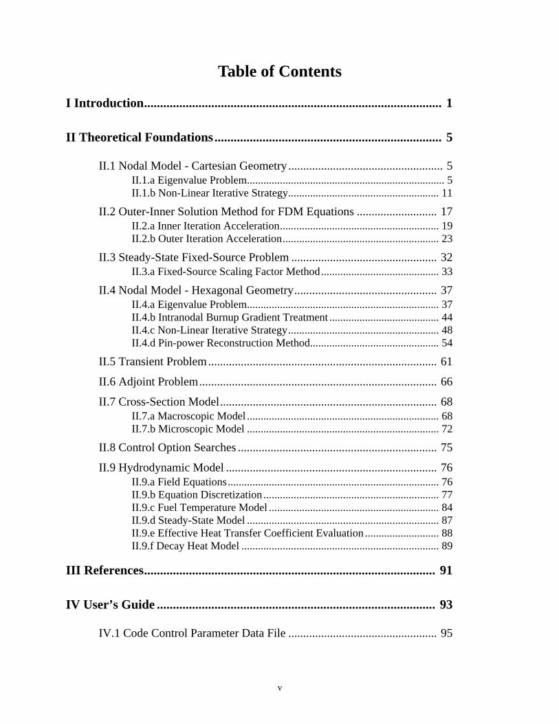
Table of Contents
I Introduction............................................................................................. 1
II Theoretical Foundations....................................................................... 5
II.1 Nodal Model - Cartesian Geometry .................................................... 5II.1.a Eigenvalue Problem........................................................................ 5II.1.b Non-Linear Iterative Strategy....................................................... 11
II.2 Outer-Inner Solution Method for FDM Equations ........................... 17II.2.a Inner Iteration Acceleration.......................................................... 19II.2.b Outer Iteration Acceleration......................................................... 23
II.3 Steady-State Fixed-Source Problem ................................................. 32II.3.a Fixed-Source Scaling Factor Method........................................... 33
II.4 Nodal Model - Hexagonal Geometry................................................ 37II.4.a Eigenvalue Problem...................................................................... 37II.4.b Intranodal Burnup Gradient Treatment ........................................ 44II.4.c Non-Linear Iterative Strategy....................................................... 48II.4.d Pin-power Reconstruction Method............................................... 54
II.5 Transient Problem............................................................................. 61
II.6 Adjoint Problem................................................................................ 66
II.7 Cross-Section Model......................................................................... 68II.7.a Macroscopic Model ...................................................................... 68II.7.b Microscopic Model ...................................................................... 72
II.8 Control Option Searches ................................................................... 75
II.9 Hydrodynamic Model ....................................................................... 76II.9.a Field Equations............................................................................. 76II.9.b Equation Discretization................................................................ 77II.9.c Fuel Temperature Model .............................................................. 84II.9.d Steady-State Model ...................................................................... 87II.9.e Effective Heat Transfer Coefficient Evaluation ........................... 88II.9.f Decay Heat Model ........................................................................ 89
III References........................................................................................... 91
IV User’s Guide ....................................................................................... 93
IV.1 Code Control Parameter Data File .................................................. 95
v
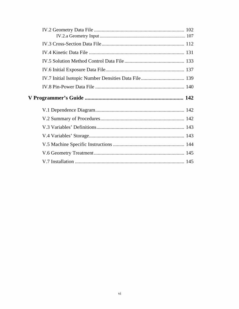
IV.2 Geometry Data File ....................................................................... 102IV.2.a Geometry Input ......................................................................... 107
IV.3 Cross-Section Data File................................................................. 112
IV.4 Kinetic Data File ........................................................................... 131
IV.5 Solution Method Control Data File ............................................... 133
IV.6 Initial Exposure Data File.............................................................. 137
IV.7 Initial Isotopic Number Densities Data File.................................. 139
IV.8 Pin-Power Data File ...................................................................... 140
V Programmer’s Guide ........................................................................ 142
V.1 Dependence Diagram...................................................................... 142
V.2 Summary of Procedures.................................................................. 142
V.3 Variables’ Definitions..................................................................... 143
V.4 Variables’ Storage........................................................................... 143
V.5 Machine Specific Instructions ........................................................ 144
V.6 Geometry Treatment ....................................................................... 145
V.7 Installation ...................................................................................... 145
vi

vii
Listing of Tables
Table 1 :Non zero entries in the 16 by 16 two-node NEM problem................. 14
Table 2 :Values of g2(u) as a function of u....................................................... 41
Table 3 :Values of g(u,0) as a function of u...................................................... 43
Table 4 :List of required file names. ................................................................. 94
Table 5 :Listing of procedures and their functions. ........................................ 156
Table 6 :Listing of fcb files containing named COMMON blocks................. 168
Table 7 :Sample interactive session with NESTLE.DICT.............................. 169

viii
Listing of Figures
Figure 1: Overview of NESTLE nested iterative solution strategy. ................. 29
Figure 2: Hex geometry dimensions and axis orientation................................. 37
Figure 3: Conformal mapping of a hexagon to a rectangle............................... 38
Figure 4: v- vs. y-coordinates at x=R(30.5/2). .................................................. 47
Figure 5: Mapping scale function at u=a/2........................................................ 47
Figure 6: Corner Flux Configuration. ............................................................... 58
Figure 7: Thermal-hydraulic mesh notation...................................................... 79
Figure 8: Radial material geometry figures for different core geometries...... 109
Figure 9: Dependence diagram of the NESTLE code..................................... 147

tion
ty);
nvalue
ution
bles:
ernal
gard to
(
Three,
ilable,
core
dary
the
d by a
nodal
etric,
axial
I. Introduction
NESTLE is a FORTRAN77 code that solves the few-group neutron diffusion equa
utilizing the Nodal Expansion Method (NEM). NESTLE can solve the eigenvalue (criticali
eigenvalue adjoint; external fixed-source steady-state; or external fixed-source or eige
initiated transient problems. The code name NESTLE originates from the multi-problem sol
capability, abbreviatingNodal Eigenvalue,Steady-state,Transient,Le core Evaluator. The
eigenvalue problem allows criticality searches to be completed on one of the following varia
soluble boron, coolant inlet temperature, control rod position or core power level. The ext
fixed-source steady-state problem can also search on these same parameters, now in re
achieving a specified power level.
Two or four energy groups can be utilized, with all groups being thermal groupsi.e.
upscatter exists) if desired. Core geometries modelled include Cartesian and Hexagonal.
two and one dimensional models can be utilized. Various core symmetry options are ava
including quarter, half and full core for Cartesian geometry and one-sixth, one-third and full
for Hexagonal geometry. Zero flux, non-reentrant current, reflective and cyclic boun
conditions are treated
The few-group neutron diffusion equation is spatially discretized utilizing theNodal
Expansion Method (NEM). For Cartesian geometry, quartic polynomial expansion for
transverse integrated fluxes are employed. Transverse leakage terms are represente
quadratic polynomial. For Hexagonal geometry, a conformal mapping based hexagonal
method is employed. The transverse integrated flux expansion consists of trigonom
hyperbolic trigonometric, and polynomial functions. The transverse leakage term in the
1

ed in
xagon.
oups.
ation,
g a
tically
e the
Shift
lerate
ndent
ter and
od is
ments
lation.
tegy,
up
ither
ergy
direction is represented by a quadratic polynomial while the radial contribution is express
terms of the mapping scale function and the physical currents on the surfaces of the he
DiscontinuityFactors (DFs) are utilized to correct for homogenization errors.
Transient problems utilize a user specified number of delayed neutron precursor gr
Time dependent inputs include coolant inlet temperature and flow; soluble poison concentr
and control banks’ positions. Time discretization is done in a fully implicit manner utilizin
first-order difference operator for the diffusion equation. The precursor equations are analy
solved assuming the fission rate behaves linearly over a time-step.
Independent of problem type, an outer-inner iterative strategy is employed to solv
resulting matrix system. Outer iterations can employ Chebyshev acceleration, Weilandt
acceleration with flux extrapolation, and the Fixed Source Scaling Technique to acce
convergence. Inner iterations employ either color line or point SOR iteration schemes, depe
upon problem geometry. Values of the energy group dependent optimum relaxation parame
the number of inner iterations per outer iteration to achieve a specified L2 relative error reduction
are determined a priori. The non-linear iterative strategy associated with the NEM meth
utilized. This has advantages in regard to reducing FLOP count and memory size require
versus the more conventional linear iterative strategy utilized in the surface response formu
In addition, by electing to not update the coupling coefficients in the nonlinear iterative stra
the Finite DifferenceMethod (FDM) representation, utilizing the box scheme, of the few-gro
neutron diffusion equation results. The implication is that NESTLE can be utilized to solve e
the nodal or FDM representation of the few-group neutron diffusion equation.
Thermal-hydraulic feedback is modelled employing aHomogenousEquilibrium M ixture
(HEM) model, allowing two-phase flow to be treated. However, only the continuity and en
2
sumed
eter
ourant
ially
in a
y heat.
ation
d that
on to
e code
ed to
ized by
s
ictor-
the
ed and
t the
ptions
or
olant
ensity.
equations for the coolant are solved, implying a constant pressure treatment. The slip is as
to be one in the HEM model. The fuel temperature is determined utilizing a lumped param
model. The SETS method is used for the temporal treatment to overcome the material C
limit on numerical stability. A conventional staggered mesh formulation is used in spat
discretizing the fluid’s equations. Flow is assumed to be parallel to the axial direction with
closed channel. A user specified number of decay heat groups are used to model deca
Direct deposition in the coolant of fission energy is accounted for. Equation of State inform
is provided via polynomials, whose coefficients are provided as input. It should be recognize
the thermal-hydraulic model was developed with a pin-cell geometry as its basis. Adopti
other geometries, such as appear in gas-cooled reactors, would likely require some sourc
modifications.
The thermal conditions predicted by the thermal-hydraulic model of the core are us
correct cross-sections for temperature and density effects. Cross-sections are parameter
color, control rod state (i.e. in or out) and burnup, implying fuel burnup modelling capabilitie
exist. Either a macroscopic or microscopic fuel depletion model may be employed. A Pred
Corrector formulation is used to solve the depletion equations. With the election of
microscopic option, depletion equations for the U234 through U236 and U238 through Pu242
depletion chains, two lumped fission product groups, and a simple burnable poison are solv
used in conjunction with burnup dependent microscopic cross-sections to construc
macroscopic cross-sections. The I-Xe and Pm-Sm chains are also modelled, with various o
to determine their number densities (i.e. equilibrium, transient, peak Sm-no Xe, no Sm nor Xe,
frozen). All cross-sections are characterized in terms of a Taylor’s series expansion in co
density, coolant temperature, effective fuel temperature, and soluble poison number d
3

ut.
uracy.
n is
oups
flux,
n to
tion is
art file
n of
tainer
Taylor’s series terms utilized (e.g. linear or quadratic in coolant density) are specified via inp
An intranodal cross section treatment can be used with Hexagonal geometry to improve acc
Pin power reconstruction is available for Hexagonal geometry. A two-group formulatio
utilized to complete pin-power reconstruction independent of whether two or four energy gr
are utilized in solving the neutron diffusion equation.
Output edits include predicted values of the key core attributes, such as power,
temperatures, isotopic number densities and burnup spatial distributions, in additio
documenting key input options and convergence behavior parameters. The output informa
biased towards the sort of information a nuclear designer of a power reactor requires. A rest
is written, allowing restart for branch cases, re-initiation of core depletion, continuatio
iterations towards a tighter convergence, or re-initiation of a transient.
Memory management is accomplished via a container array. Code determined con
array pointers are used to facilitate problem specific memory allocation (e.g.trading off of spatial
and energy detail within a fixed total memory size).
4

the
[1,2].
f the
sverse
tion,
d
and,
tron
II. Theoretical Foundations
II.1. Nodal Model - Cartesian Geometry
II.1.a. Eigenvalue Problem
The following section describes the standard NEM formulation for the solution of
three-dimensional, Cartesian geometry, multi-group, eigenvalue neutron diffusion equation
The principal characteristics of the polynomial nodal method are its quartic expansions o
one-dimensional transverse-integrated flux and quadratic leakage model for the tran
leakage.
Consider the general form of the steady-state multi-group neutron diffusion equa
written in standard form and with the group constants (i.e. properly weighted cross-sections an
discontinuity factors) already available from a lattice physics calculation forg = 1, 2,..., G
(1)
where the dependence of each quantity on the spatial coordinate has been suppressed,
Dg= diffusion coefficient [cm]
φg= neutron flux [cm-2sec-1]
Σtg = total macroscopic cross section [cm-1]
Σsgg’= group-to-group scattering cross section [cm-1]
χg= fission neutrons yield
k= multiplication factor (i.e. critical eigenvalue)
vg= average number of neutrons created per fission
Σfg= macroscopic fission cross section [cm-1]
As with most modern nodal methods, we begin by intergrating the multi-group neu
∇– Dg∇φg Σtgφg+⋅ Σsgg′φg′χg
k----- vg′Σ fg′φg′
g′ 1=
G
∑+g′ 1=
G
∑=
r
5

s. For
, the
x-
in
diffusion equation over a material-centered spatial node which has homogenized propertie
Cartesian geometry we rewrite Eqn. (1) for the arbitrary spatial nodel,
(2)
where, , and
For simplicity, in cases where redundant equations exist in all three directions
illustrating equations will be only given in the x-direction. Using Fick’s Law, which in the
direction can be expressed as,
(3)
where,
allows Eq. (2) to be rewritten as:
(4)
Integration of Eq. (4) over the volume of nodel generates a local neutron balance equation
terms of the face-averaged net currents and the node volume average flux.
(5)
D– gl
x2
2
∂∂ φg
l r( ) Dgl
y2
2
∂∂ φg
l r( )– Dgl
z2
2
∂∂ φg
l r( ) Agl φg
l r( )+– Qgl r( )=
g 1 G,( )∈
r( ) x y z, ,( ) Vl∈≡ x y∆ z∆∆ Volume of nodel≡=
Agl Σtg
l Σsggl
–xg
l
k-----vgΣ fg
l–=
Qgl
r( ) Qgg′l φg′
lr( )
g′ g≠
G
∑ Σsgg′l φg′
lr( )
xgl
k----- vg′Σ fg′
l φg′l
r( )g′ g≠
G
∑+g′ g≠
G
∑==
jgxl
r( ) Dgl
x∂∂ φg
lr( )–=
jgxl
r( ) x-component of the net neutron current≡
x∂∂
jgxl
r( )y∂
∂jgyl
r( )z∂
∂jgzl
r( ) Agl φg
lr( )++ + Qg
lr( )=
1
xl∆
-------- Lgxl
( ) 1
yl∆
------- Lgyl
( ) 1
zl∆
------- Lgzl
( ) Agl φg
l+ + + Qg
l=
6

ted
en in
ome
It is the
lation
three-
. This
, of the
where, assuming nodel is centered around the coordinate’s origin, the volume integra
quantities are defined below:
and,
where,
Eq. (5) is known as the nodal balance equation. Now for the neutron diffusion equation writt
this form, in order to obtain the spatial neutron flux distribution, one must devise s
relationship between the node average flux and the face-averaged net (surface) currents.
equations used to compute the surface currents in Eq. (5) which distinguish one nodal formu
from another. In NEM, the widely used method of transverse-integration is used, where the
dimensional diffusion equation is integrated over the two directions transverse to each axis
generates three one-dimensional equations, one for each direction in Cartesian coordinates
following form,
φgl 1
Vl
----- φgl
r( ) x y z Node volume average flux≡ddd
z∆ l
2-------–
z∆ l
2-------
∫y∆ l
2-------–
y∆ l
2-------
∫x∆ l
2-------–
x∆ l
2-------
∫=
Qgl 1
Vl
----- Qgl
r( ) x y z Node volume average source≡ddd
z∆ l
2-------–
z∆ l
2-------
∫y∆ l
2-------–
y∆ l
2-------
∫x∆ l
2-------–
x∆ l
2-------
∫=
1
xl∆
--------Lgxl 1
xl∆
-------- Jgx+l
Jgx-l
–( ) 1
Vl
-----x∂
∂jgxl
r( ) x y zddd
z∆ l
2-------–
z∆ l
2-------
∫y∆ l
2-------–
y∆ l
2-------
∫x∆ l
2-------–
x∆ l
2-------
∫= =
Jgx ±l
Average x-directed net current on node facesx∆ l
2--------±≡
7

as a
such
(6)
where,
and,
In NEM, the one-dimensional averaged flux that appears in Eq. (6), is expanded
general polynomial,
(7)
where is the node average flux, implying for Eq. (7) to be true that must be chosen
that the basis functions satisfy
(8)
Note that for quartic NEM, the method used in NESTLE, the summation extends toN = 4. The
first four basis functions in NEM can be expressed as follows [1],
(9)
which can be shown to also satisfy the following,
xdd
jgxl
x( ) Agl φgx
l+ x( ) Qgx
lx( ) 1
yl∆
-------Lgyl
x( )–1
zl∆
-------Lgzl
x( )–=
Lgyl
x( ) 1
zl∆
-------y∂
∂jgyl
r( ) y z Average y-direction transverse leakage≡dd
yl∆2
-------–
yl∆2
-------
∫zl∆2
-------–
zl∆2
-------
∫=
Lgzl
x( ) 1
yl∆
-------z∂
∂jgzl
r( ) z y Average z-direction transverse leakage≡dd
zl∆2
-------–
zl∆2
-------
∫yl∆2
-------–
yl∆2
-------
∫=
φgxl
x( ) φgl
agxnl
f n x( )n 1=
N
∑+=
φgl
f n x( )
f n x( ) xd
x∆ l
2-------–
x∆ l
2-------
∫ 0 for n 1 ...,N,= =
x
xl∆
-------- ; 3
x
xl∆
-------- 2 1
4---;–
x
xl∆
-------- 3 1
4--- x
xl∆
-------- ;–
x
xl∆
-------- 4 3
10------ x
xl∆
-------- 2
– 180------+
f1 f2 f3 f4
8

total
e node
roup,
ides
ts from
nergy
any
h
me [3]
oment
ctions,
, and
nsion
(10)
At this point it is appropriate to consider the elementary concept of accounting for the
number of equations and that of unknowns. For a three-dimensional Cartesian geometry, th
average andN expansion coefficients in each direction appear per node per energy g
implying a total of 3N+1 equations are required. The nodal balance equation, Eq. (5), prov
one equation, where now Eqs. (3) and (7) are used to eliminate face-averaged net curren
this equation. Surface current and flux continuity provide 6 more equations per node per e
group. So forN=2, there would be an equal number of equations and unknowns without
further development. However, forN= 4, two additional unknowns are introduced for eac
direction per node per energy group. This is addressed by using a weighted residual sche
applied to Eq. (6), which in essence provides the additional equations (referred to as the m
equations) needed,
(11)
where the two weighting functions for n = 1,2 are chosen to be the same as the basis fun
namelyωn(x) = fn(x), as those used in the one-dimensional flux expansion1. Here, the first and
second (actually linear combination of zeroth and second) moments of the flux, source
leakage for each groupg are defined by,
The first term in Eq. (11) is evaluated by using Eqs. (3) and (7) and the definition of the expa
1. This constitutes amoments weightingscheme; if one usesωn(x) = fn+2(z) for n = 1,2 it is known asGaler-kin weighting. Numerical experiments favormoments weighting.
f nx
l∆2
--------± 0 for n 3 4,==
ω< n x( )xd
djgxl
x( ) Agl φgxn
l+>, Qgxn
l 1
yl∆
-------Lgyxnl
–1
zl∆
-------Lgzxnl
–=
ωn x( ) φgxl
x( ), >< ωn x( ) Qgxl
x( ), >< ωn x( ) Lgyl
x( ), >< ωn x( ) Lgzl
x( ),< >
φ lgxn Ql
gxn Llgyxn Llgzxn
9
re the
known,
dratic
the y-
e
g the x-
odes.
coefficients, and completing the integration (i.e. inner product) analytically.
One last point which needs to be addressed before Eq. (11) can be solved a
transverse leakage terms appearing on the right hand side. Their spatial dependency is un
so their “shape” must be approximated. The most popular approximation in NEM is the qua
transverse leakage approximation. For example, the x-direction spatial dependence of
direction transverse leakage is approximated by,
(12)
where is the average y-directed leakage in nodel, and the coefficients and can b
expressed in terms of average y-directed leakages of the two nearest-neighbor nodes alon
direction (i.e. nodesl-1 andl+1) so as to preserve the node average leakages of these three n
The quadratic expansion coefficients can be shown to be given by,
(13)
(14)
where,
(15)
Lgyl
x( ) Lgyl
ρgy1l
f 1 x( ) ρgy2l
f 2 x( )+ +≅
Lgyl
ρgy1l ρgy2
l
ρgy1l
gl
xl∆( ) Lg
l 1+Lg
l–( ) x
l∆ 2 xl 1–∆+( ) x
l∆ xl 1–∆+( ) Lgy
lLgy
l 1––( ) x
l∆ 2 xl 1+∆+( ) x
l∆ xl 1+∆+( )+[ ]=
ρgy2l
gl
xl∆( )
2Lgy
l 1+Lgy
l–( ) x
l∆ xl 1–∆+( ) Lgy
l 1–Lgy
l–( ) x
l∆ xl 1+∆+( )+[ ]=
gl
xl∆ x
l 1+∆+( ) xl∆ x
l 1–∆+( ) xl 1–∆ x
l∆ xl 1+∆+ +( )[ ]
1–=
10

the
nd to
on,
mith
de
rather
(
oup
tegy,
alled
ing
oved
mated
dated
This
orces
rents
rage
forms;
usable
e base
actor
II.1.b. Non-Linear Iterative Strategy
The most common manner of solving the matrix system associated with NEM is
response-matrix formulation. To minimize computer run time and memory requirements, a
facilitate the capability to solve either the NEM or Finite Difference Method (FDM) formulati
the non-linear iterative strategy is employed in NESTLE. This technique was developed by S
[4,5,6] and successfully implemented into the Studsvik QPANDA and SIMULATE co
packages. The documentation available on this technique is scarce, but it turns out to be
simplistic and almost trivial to implement in a FDM code which utilizes the box-schemei.e.
material-centered).
The basic idea is applicable to the standard FDM solution algorithm of the multi-gr
diffusion equation. Solving the FDM based equation utilizing an outer-inner iterative stra
every outer iterations (where is somewhat arbitrary but can be optimized) the so-c
“two-node problem” calculation (a spatially-decoupled NEM calculation spanning two adjoin
nodes) is performed for every interface (for all nodes and in all directions) to provide an impr
estimate of the net surface current at that particular interface. Subsequently, the NEM esti
net surface currents are used to update (i.e. change) the original FDM diffusion coupling
coefficients. Outer iterations of the FDM based equation are then continued utilizing the up
FDM coupling coefficients for outer iterations. The entire process is then repeated.
procedure of updating the FDM couplings is a convergent technique which progressively f
the FDM equation to yield the higher-order NEM predicted values of the net surface cur
while satisfying the nodal balance Eq. (5), thus yielding the NEM results for the node-ave
flux and fundamental mode eigenvalue. The advantages of this technique come in many
the storage requirements are minimal because the two-node problem arrays are re-
(disposable) at each interface, the rate of convergence is nearly comparable to that of th
FDM algorithm being used, the number of iteratively determined unknowns is reduced by a f
N∆ 0 N∆ 0
N0∆
11

e of
n be
icity,
ions
terms
he x-
/node
with
ment
cond
of 6 (node flux vs. partial surface current), and the simplicity of the algorithm and eas
implementation, compared to any other nodal technique, is far superior.
The two-node problem produces an 8G X 8G linear system of equations which ca
constructed by applying the standard NEM relations to two adjoining nodes. For simpl
consider two arbitrary adjoining nodes in the x-direction. Denote these notes asl andl+1:
Substitution of the one-dimensional expansion, Eq. (7), into Fick’s law yields express
for the average x-direction net surface currents at the left(-) and right(+) interfaces of nodel,
(16)
Now, assume the node average flux, criticality constant, and all transverse direction
are known from a previous iteration; then, the total number of unknowns associated with t
direction two node problem is 8G, which corresponds to the 4 expansion coefficients/group
(x) G groups (x) two nodes. The 8G constraint equations are obtained as follows. We begin
the substitution of Eq. (16) into the nodal balance equation for node l, to yield the zeroth mo
constraints (G equations/node),
(17)
A similar substitution into the moment-weighted equation, Eq. (11), yields the first and se
moment constraints (2G equations/node),
(18)
(19)
Nodel
Nodel+1x- x+
jgx±l D– g
l
xl∆
---------- agx1l
3agx2l 1
2---agx3
l 15---agx4
l±+±≡
D– gl
xl∆ x
l∆---------------- 6agx2
l 25---agx4
l+
1
yl∆
-------Lgyl
–1
zl∆
-------Lgzl
Agl φg
lQgg′
l
g′ g≠
G
∑ φg′l
+––=
60
xl∆
--------Dg
l
xl∆
-------- Agl
+ agx3l
Qgg′l
ag′x3l
g′ g≠
G
∑ 10Aglagx1
l– 10 Qgg′
lag′x1
l
g′ g≠
G
∑+– 101yl∆
--------ρgy1l 1
zl∆-------ρgz1
l+
=
140
xl∆
---------Dg
l
xl∆
-------- Agl
+ agx4l
Qgg′l
ag′x4l
g′ g≠
G
∑ 35Aglagx2
l– 35 Qgg′
lag′x2
l
g′ g≠
G
∑+– 351yl∆
--------ρgy2l 1
zl∆-------ρgz2
l+
=
12

The
using
ons)
q. (7),
sics
of the
tially
t each
t the
t of a
ly [7].
=2.
Similar equations can be written for node l+1, producing a total of 6G equations.
continuity of net surface current constraints at the interface (G equations) are obtained by
Eq. (16) at the adjoining interface of the two nodes,
(20)
Last, the continuity (or discontinuity) of surface-averaged flux constraints (G equati
are obtained by equating the surface-averaged fluxes of the two adjoining nodes by using E
(21)
where and are the Discontinuity Factors (DFs) obtained from lattice phy
calculations. Do note that continuity conditions are never imposed on the outside surfaces
two-node problem, since the two-node problem is deliberately formulated to be spa
decoupled. Continuity is assured in the formulation of the FDM based equations.
Eqs.(7) through (21) constitute the 8G system of equations needed to be solved a
interface. This matrix system, after taking advantage of its reducability and by noting tha
even-moment expansion coefficients don’t change whether the node is on the left or righ
two-node problem, can be reduced to smaller systems which can be solved quite efficient
The following table illustrates this more efficient arrangement of unknowns for the case of G
D– gl
xl∆
---------- agx1l
3agx2l agx3
l
2----------
agx4l
5----------+ + +
D– gl
xl 1+∆
--------------- agx1l 1+
3agx2l 1+ agx3
l 1+
2-----------
agx4l 1+
5-----------–+–=
dgx +l φg
l agx1l
2----------
agx2l
2----------+ + dgx –
l 1+ φgl 1+ agx1
l 1+
2-----------
agx2l 1+
2-----------+–=
dgx ±l
dgx ±l 1+
13

8G
duce
cient
*Refers to order of polynomial that transverse integrated
flux expansion coefficient is associated with.
In NESTLE, the two-node problems are solved by utilizing the analytic solution to the 8G X
matrix system. This was accomplished by employing symbolic manipulator software to pro
the FORTRAN code segment used in NESTLE. This approach is computationally more effi
Table 1: Non zero entries in the 16 by 16 two-node NEM problem.
Eqn Grp Nod a b c d e f g h i j k l m n o p
0th Moment 1 l x x
0th Moment 2 l x x
2nd Moment 1 l x x x x
2nd Moment 2 l x x x x
0th Moment 1 l+1 x x
0th Moment 2 l+1 x x
2nd Moment 1 l+1 x x x x
2nd Moment 2 l+1 x x x x
1st Moment 1 l x x x x
1st Moment 2 l x x x x
1st Moment 1 l+1 x x x x
1st Moment 2 l+1 x x x x
Cur Con 1 x x x x x x x x
Cur Con 2 x x x x x x x x
Flx Dis 1 x x x x
Flx Dis 2 x x x x
UNKNOWN NODE GROUP EXP. COEF.*
a l 1 2b l 2 2c l 1 4d l 2 4e l+1 1 2f l+1 2 2g l+1 1 4h l+1 2 4i l 1 1j l 2 1k l 1 3l l 2 3m l+1 1 1n l+1 2 1o l+1 1 3p l+1 2 3
14

to
-node
-node
e
n all
wn in
nt, the
be
is
FDM
ere to
is
dard
LE,
d. The
rface
than utilizing a direct matrix solver (e.g. LU decomposition); however, it limits the values of G
those directly programmed for. Also note that on boundaries special treatments of the two
problems are required. Depending upon the specified boundary condition (BC), one
problems may originate (e.g. zero flux BC), or on interior axis geometry unfolding may b
required to create a two-node problem (e.g. cyclic BC).
Solutions of the two-node problems provide NEM evaluated values of the currents o
surfaces for specified values of the node average fluxes [recall they were assumed kno
solving the two-node problems]. To correct the FDM based expression for the surface curre
following approach is utilized. The coupling coefficient update to the FDM equation can
implemented by simply expressing the FDM net surface current at thex+ face of nodel as
follows,
(22)
The first term on the RHS is the normal FDM approximation for a box scheme, where
the actual FDM diffusion coupling coefficient between nodes l and l+1,
(23)
The second term on the RHS represents the nonlinear NEM correction applied to the
scheme. The (+) sign between the flux values in the second term of Eq. (22) is purposely th
improve the convergence behavior of the nonlinear iterative method [8]. Note that if
zero, which it initially is in NESTLE’s implementation, then Eq. (22) corresponds to the stan
FDM definition of the net surface current. This is the basis for the FDM option within NEST
where now two-node problem solves and coupling coefficients updates are never complete
value of is determined by setting Eq. (22) equal to the NEM two-node predicted su
Jgx +l FDM, Dgx +
l FDM,
xl∆ x
l 1+∆+2
-----------------------------
-----------------------------– φgl 1+
φgl
–[ ]Dgx +
l NEM,
xl∆ x
l 1+∆+2
-----------------------------
----------------------------- φgl 1+
φgl
+[ ]–=
Dgx +l FDM,
Dgx +l FDM, Dg
lDg
l 1+x
l∆ xl 1+∆+( )
Dgl
xl∆ Dg
l 1+x
l 1+∆+------------------------------------------------------=
Dgx +l NEM,
Dgx +l NEM,
15

r this
one
n for
inally,
n the
current value, using the associated node average flux values in Eq. (22) and solving fo
quantity.
Summarizing, to apply a NEM update after outer iterations of the FDM routine,
solves the two-node problem at a given interface, then (with the expansion coefficients know
that interface) one calculates the NEM estimate of the net surface current using Eqn.(16) F
one equates this result to Eq. (22), and solves for the value of which will be used i
subsequent set of FDM iterations.
N0∆
Dgx +l NEM,
16
DM
ting,
stem.
tion,
and
tions
lems
the
TLE’s
the
onal
(23)
. (8)
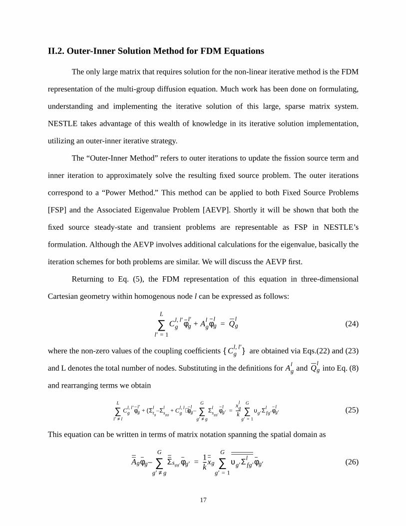
II.2. Outer-Inner Solution Method for FDM Equations
The only large matrix that requires solution for the non-linear iterative method is the F
representation of the multi-group diffusion equation. Much work has been done on formula
understanding and implementing the iterative solution of this large, sparse matrix sy
NESTLE takes advantage of this wealth of knowledge in its iterative solution implementa
utilizing an outer-inner iterative strategy.
The “Outer-Inner Method” refers to outer iterations to update the fission source term
inner iteration to approximately solve the resulting fixed source problem. The outer itera
correspond to a “Power Method.” This method can be applied to both Fixed Source Prob
[FSP] and the Associated Eigenvalue Problem [AEVP]. Shortly it will be shown that both
fixed source steady-state and transient problems are representable as FSP in NES
formulation. Although the AEVP involves additional calculations for the eigenvalue, basically
iteration schemes for both problems are similar. We will discuss the AEVP first.
Returning to Eq. (5), the FDM representation of this equation in three-dimensi
Cartesian geometry within homogenous nodel can be expressed as follows:
(24)
where the non-zero values of the coupling coefficients are obtained via Eqs.(22) and
and L denotes the total number of nodes. Substituting in the definitions for and into Eq
and rearranging terms we obtain
(25)
This equation can be written in terms of matrix notation spanning the spatial domain as
(26)
Cgl l ′, φg
l ′
l ′ 1=
L
∑ Agl φg
l+ Qg
l=
Cgl l ′,
Agl
Qgl
Cgl l ′,
l ′ l≠
L
∑ φgl ′
Σtg
l Σsgg
lCg
l l,+–( )+ φg
lΣsgg′
l
g′ g≠
G
∑ φg′l
–xg
l
k----- υg′
g′ 1=
G
∑ Σ fg′l φg′
l=
Agφg Σsgg′φg′g′ g≠
G
∑–1k---xg υg′Σ fg′
l φg′g′ 1=
G
∑=
17

has a
X L)
GL)
ps.
y Eq.
es for
ive
e rate
ups,
plies
where the “bar” over the node average flux value now denotes a column vector. Matrix
seven-banded matrix structure for three-dimensional Cartesian geometry. In turn, the G (L
matrix systems expressed by Eq. (26) can be collected to write the following single (GL X
matrix system.
(27)
The matrix is block lower triangular in structure for that portion applicable to the fast grou
The outer-inner iteration process is summarized as follows: For the AEVP specified b
(27), given an arbitrary initial vector , the outer iterations generate successive estimat
the flux vector by the process
(28)
where how the criticality constant (i.e.eigenvalue) is updated will be discussed later. The iterat
matrix associated with the outer iterations is
(29)
The properties of the iterative matrix has a significant role in determining the convergenc
of the power iterations [9,10].
In solving Eq. (28), advantage is taken of the structure of the matrix. For the fast gro
solving from low to high energy group number results in energy group decoupling. This im
that we may solve a system of linear equations of the form
(30)
where,
(31)
Ag
Aφ 1k---Fφ=
A
φ0( )
φ
φq( ) 1
kq 1–( )---------------A
1–Fφ
q 1–( )=
Q A1–F=
Q
A
Agφgq( )
Sgq( )
=
Sgq( ) Σsgg′φg′
q( ) 1
kq 1–( )---------------+
g′ g≠
G
∑ χg νg′Σ f g′φg′q 1–( )
g′ 1=
G
∑=
18

oups
g Eqn.
ups’
attering
lor
ions.
ree-
direct
of
llows.
For the thermal groups, NESTLE assumes the group fluxes for all other thermal gr
except the one being updated are known. This produces energy group decoupling, allowin
(30) to be utilized. So called “scattering” iterations are then completed after all thermal gro
fluxes are updated. Stationary acceleration is employed to accelerate convergence of the sc
iterations.
II.2.a. Inner Iteration Acceleration
To solve Eq. (30) we introduce the inner iterations. In this work we employ a Multi-Co
Point or Line SOR Method, depending upon problem geometry, for the inner iterat
Specifically, a Red-Black Point or Line SOR method is used in NESTLE for two or th
dimensional Cartesian geometry, respectively. For one-dimensional Cartesian geometry, a
matrix solve is utilized since the group-wise A matrix is triangular allowing employment
Gaussian elimination.
Mathematically, this approach is a multi-splitting method and can be expressed as fo
(32)
where,
(33)
and
(34)
(35)
φ φp where vectorφp spans nodes of color ''p''⊕=
φpm 1+( )
Bp1–
S Cpp′φp′m 1+( )
Cpp′φp′m( )
p′ p 1+=
P
∑+p′ 1=
p 1–
∑+= for p 1,2,...,P=
A Ap and non-square matrixAp equals rows ofA that span nodes of color ''p''⊗=
Ap Bp Cpp′
p′ p≠
P
∑–= for p = 1,2,...,P
φpm 1+( )
φpm( )
ω φpm 1+( ) φp
m( )–( )+=
19

in the
cheme
that
per
error
that the
since
ese
ptable.
ss-
he
arizes
lue of
nergy
Note that the group g and outer iteration count (q) indices have been suppressed for clarity
above equations. The matrix is square and has either a diagonal structure for the point s
or block diagonal structure composed of tridiagonal blocks for the line scheme. This implies
the action of indicated in Eqs. (32) is simple to evaluate. A total of inner iterations
outer iterations are completed, this value determined such that the specified relative
reduction from the 0th iterative error for the inner iterations is achieved.
To a priori determine the value of the optimum relaxation parameter,ω and [which
are energy group dependent but dependence notation has been surpressed], it is assumed
iterative matrix associated with this inner iterative method is symmetrizable. This is not true
the NEM corrections to the FDM coupling coefficients invalidate symmetry; however, th
corrections have been found to be relatively small so the symmetrizable assumption is acce
Making this assumption, we can expressω in terms of the spectral radius of the associated Gua
Seidel iteration matrix, , as follows,
(36)
Clearly . Therefore, calculation of the spectral radius of t
associated Gauss-Seidel iterative matrix is the heart of this procedure. The following summ
the details of the computational procedure used in NESTLE to obtain an estimate of the va
ω, which is based upon the DIF3D methodology [10]. These steps are completed for each e
group.
Bp
Bp1–
NI∆
NI∆
ρ LG-S
( )
ω 2
1 1 ρ LG-S( )–[ ]
1/2+
------------------------------------------------=
LG-S
LSOR
ω( )with ω 1= =
20

st
d
0.1 Step 1.Starting with an arbitrary non-negative initial guess vector , complete at lea
ten Gauss-Seidel iterations in solving the following equation.
0.2 Step 2.Following each iteration withm >10, estimate the upper and lower bounds of the
spectral radii using the following equations.
Compute the corresponding relaxation factors given by
0.3 Step 3.Terminate iteration when either
or mequals a specified upper limit [10,11]. The optimum factorω is then set toω(m). This
test forces tighter convergence ofω when is close to unity to ensure the require
numerical accuracy is achieved.
x0( )
Ax 0=
λ m( ) xm( )
xm( )
,⟨ ⟩
xm( )
xm 1–( )
,⟨ ⟩-----------------------------------≡
λm( )
MAXixi
m( )
xim 1–( )----------------≡
λ m( )MINi
xim( )
xim 1–( )----------------≡
ω m( ) 2
1 1 λ m( )–[ ]
1/2+
---------------------------------------≡
ω m( ) 2
1 1 λm( )
–[ ]1/2
+---------------------------------------≡
ω m( ) 2
1 1 λ m( )–[ ]
1/2+
---------------------------------------≡
ω m( ) ω m( )–
2 ω m( )–
5--------------------<
ρ LG-S( )
21

uch
d of
may
ation of
ner of
antial
ns has
roup.
tio of
s are
0.4 Step 4.Determine the number of inner iterations required for each outer iteration , s
that the value of satisfies the following equation:
where
and denotes the desired relative error reduction from the initial iteration to the en
-th iteration. It is suggested that a very small number for not be used since it
force excessive inner iterations [10].
The advantages of these accelerations strategies are clear. The automated determin
the optimum overrelaxation factors relieves users of the burden of the trial and error man
specifying optimum parameters for a large class of reactor models. In addition, subst
computational time can be saved since the need to check the convergence of inner iteratio
been removed by using a fixed number of predetermined inner iterations for each energy g
The outer iterations defined by Eq. (28) are slow to converge, since the dominance ra
the iterative matrix, Eq. (29), is close to one. Two complementary acceleration technique
utilized in NESTLE to accelerate the outer iterations of the AEVP.
NI∆
NI∆
LSOR
ω( )( )NI 1–∆
LG S–
⋅ t2 NI 1–∆2
t2 NI∆2
+[ ]1/2
εin≤=
t NI∆ ω 1–[ ]NI 1–∆
2------------------
ρ LG S–
( )[ ]1/2
1 NI 1–∆( )+ 1 ρ LG-S
( )–( )1/2
[ ]=
εin
NI∆ εin
22

ased
. No
s the
yshev
ctors
od [9,
ressed
hod.
ction
yshev
in the
,
lied to
h to
II.2.b. Outer Iteration Acceleration
The outer iterations for the AEVP are accelerated by using either a polynomial b
acceleration method or an eigenvalue shift acceleration method with flux extrapolation
knowledge of higher eigenvalues are required to utilize either method. We first discus
polynomial based acceleration method, which utilizes Chebyshev polynomials. Cheb
polynomials [12] are used to obtain the best linear combinations of the previous iterative ve
so as to minimize the error. The method implemented is the Chebyshev Semi-Iterative meth
10, 11, 13]. In this method, the error vector associated with the acceleration method is exp
in terms of a linear combination of the error vectors of the underlying interactive met
Acceleration of the iteration is achieved by minimizing the error vector by appropriate sele
of the expansion coefficients, which is determined to be those associated with Cheb
polynomials. Further details of the mathematical background of this method can be found
related references [9, 10].
Since the rate of convergence in the AEVP is dependent on the dominance ratio
the Chebyshev acceleration method detailed in Refs. [9, 10, 11, 13] can therefore be app
iterations,
(37)
provided that a suitable estimate of is obtained. NESTLE follows the DIF3D approac
solve the AEVP in which we accelerate the fission sourceΨ [13], whereΨ is defined as
(38)
The accelerated iterative procedure can then be expressed as follows:
(39)
σ Q
φq( ) 1
kq 1–( )---------------Qφ
q 1–( )=
σ Q
Ψ νg′Σ fg′φg′g′ 1=
G
∑ νΣ f φ= =
Ψn* p+( ) 1
kn* p 1–+( )
------------------------QΨn* p 1–+( )
=
23
yshev
to be
ented
trix,
are
ower
tone
are
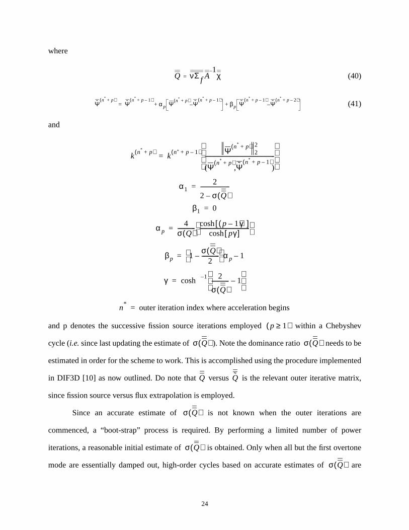
where
(40)
(41)
and
and p denotes the successive fission source iterations employed within a Cheb
cycle (i.e.since last updating the estimate of ). Note the dominance ratio needs
estimated in order for the scheme to work. This is accomplished using the procedure implem
in DIF3D [10] as now outlined. Do note that versus is the relevant outer iterative ma
since fission source versus flux extrapolation is employed.
Since an accurate estimate of is not known when the outer iterations
commenced, a “boot-strap” process is required. By performing a limited number of p
iterations, a reasonable initial estimate of is obtained. Only when all but the first over
mode are essentially damped out, high-order cycles based on accurate estimates of
Q νΣ f A1–
χ=
Ψn
*p+( )
Ψn
*p 1–+( )
αp Ψn
*p+( )
Ψ–n
*p 1–+( )
βp Ψn
*p 1–+( )
Ψ–n
*p 2–+( )
++=
kn* p+( )
kn* p 1–+( ) Ψ
n* p+( )22
Ψn* p+( )
Ψn* p 1–+( )
( , )
----------------------------------------------------
=
α12
2 σ Q( )–----------------------=
β1 0=
αp4
σ Q( )------------- p 1–( )γ[ ]cosh
pγ[ ]cosh-------------------------------------
=
βp 1σ Q( )
2-------------–
αp 1–=
γ 1–cosh 2
σ Q( )------------- 1–
=
n*
outer iteration index where acceleration begins=
p 1≥( )
σ Q( ) σ Q( )
Q Q
σ Q( )
σ Q( )
σ Q( )
24
:
ev
llest
ing
ence
w
being
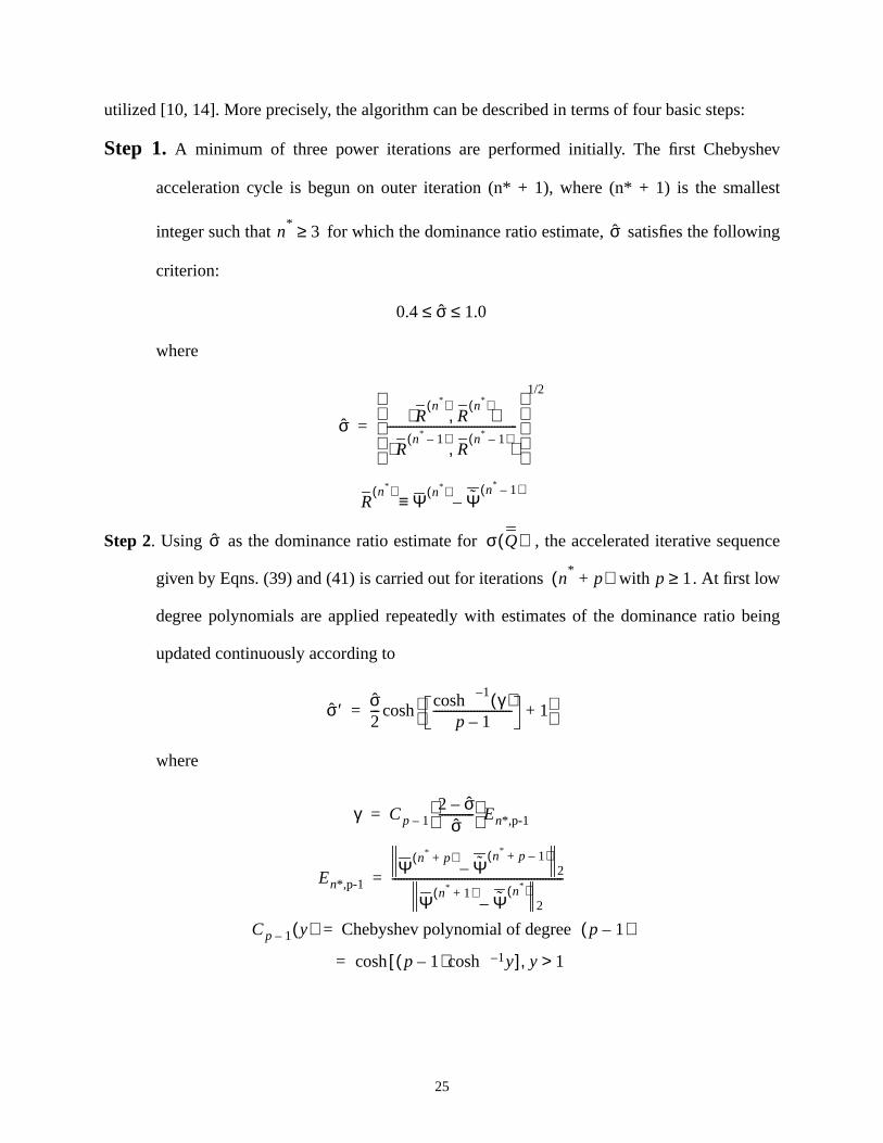
utilized [10, 14]. More precisely, the algorithm can be described in terms of four basic steps
Step 1. A minimum of three power iterations are performed initially. The first Chebysh
acceleration cycle is begun on outer iteration (n* + 1), where (n* + 1) is the sma
integer such that for which the dominance ratio estimate, satisfies the follow
criterion:
where
Step 2. Using as the dominance ratio estimate for , the accelerated iterative sequ
given by Eqns. (39) and (41) is carried out for iterations with . At first lo
degree polynomials are applied repeatedly with estimates of the dominance ratio
updated continuously according to
where
n*
3≥ σ
0.4 σ 1.0≤ ≤
σ Rn*( )
Rn*( )
,⟨ ⟩
Rn* 1–( )
Rn* 1–( )
,⟨ ⟩---------------------------------------------
1/2
=
Rn*( )
Ψ n*( ) Ψn* 1–( )
–≡
σ σ Q( )
n*
p+( ) p 1≥
σ′ σ2---
1– γ( )coshp 1–
--------------------------- 1+ cosh=
γ Cp 1–2 σ–
σ------------
En*,p-1=
En*,p-1Ψ
n* p+( )Ψ
n* p 1–+( )– 2
Ψn* 1+( )
Ψn*( )
– 2
-----------------------------------------------------------=
Cp 1– y( ) Chebyshev polynomial of degreep 1–( )=
p 1–( ) 1– ycosh[ ] y 1>,cosh=
25

ction
een
han
cycle
mial
d up
are
The polynomials are at least of degree 3 and are terminated when the error redu
factor is greater than the theoretical error reduction factor:
The theoretical error reduction factor is the error reduction which would have b
achieved if were equal to , the true dominance ratio. If is greater t
this, the acceleration cycle has not been as effective as it should have been, so a new
is started using the updated dominance ratio estimate, . Alternatively, the polyno
degree will be terminated if the reduction in theL2 relative residual of the diffusion
equation, defined as
falls below a specified value.
Step 3. After the estimates for have converged higher degree polynomials are applie
to the maximum degree specified.
Step 4.The outer iterations are terminated at outer iteration n if the following four criteria
met:
En* p, 1–
En*,p-1 Cp 1–2 σ–
σ------------
1–>
σ σ Q( ) En* p 1–,
σ′
Aφn* p+( ) 1
kn( )--------Fφ
n* p+( )–
2
1
kn* p+( )
-----------------Fφn* p+( )
2
-------------------------------------------------------------------
Aφn*( ) 1
kn( )--------Fφ
n*( )–
2
1
kn*( )
----------Fφn*( )
2
-----------------------------------------------------
--------------------------------------------------------------------
σ Q( )
26

the
ed
, the
ed to
f the
to be
effects
and are
pend
rmine
where are input parameters. The following meanings of
“normed” stopping criteria should be noted:
= L2 norm of the relative residual of the outer iterative equation
= norm of the true error of the fission source
= L2 norm of the relative residual of the diffusion equation. [Note that for a fix
source problem, whether associated with an external source or transient problem
normalization shown in the denominator of the expression bounded by is chang
theL2 norm of the source.]
Modification to this basic scheme is made in the actual implementation in NESTLE o
Chebyshev polynomial acceleration. Due to various thermal-hydraulic feedback effects,
discussed later, the coefficient matrices and in Eq. (27) are changed whenever such
are accounted for in the system. That is, since feedback effects change cross sections
dependent upon the flux solution, our matrix problem is truly non-linear since and de
upon the flux solution. Since the non-linearity is weak, one can guess a flux solution, dete
kn( )
kn 1–( )
– εk≤
Ψn( )
Ψn 1–( )
– 2
Ψn( )
Ψn 1–( )
,⟨ ⟩1/2
------------------------------------------- εΨ2≤
11 σ–------------
maxiΨi
n( ) Ψin 1–( )
–
Ψin( )---------------------------------- εΨ∞
<
Aφn( ) 1
kn( )--------Fφ
n( )–
2
1
kn( )--------Fφ
n( )
2
------------------------------------------------- εφ<
εk ε, Ψ2εΨ∞
andεφ,
εΨ2
εΨ∞L∞
εφ
εφ
A F
A F
27

flux
tions
plete
that it
. An
yshev
d. The
small
entire
in our
omial
ctions
the
rmal-
NEM
s is
, or a
hed,
latest
the feedback effects and appropriately modify and , and solve for the flux. This updated
solution can then be used to re-initiate the cycle until both the feedback and flux solu
converge. One way to handle these effects is to update the and matrices after com
termination of the outer iteration process. This approach has a clear disadvantage in
requires large computational time to obtain converged solutions for feedbacks and flux
alternate approach is to update the coefficient matrix for feedback effects during the Cheb
acceleration process. In doing so, a substantial reduction in computation time can be realize
latter approach can be justified by observing that the feedback effects are relatively
perturbations to the original system from a reactor physics point of view and hence, the
Chebyshev acceleration scheme is not jeopardized. This modified scheme is incorporated
work in such a manner that the matrices are updated just before a new Chebyshev polyn
acceleration cycle begins. The same approach is taken in regard to updating the NEM corre
to the coupling coefficients.
Figure 1 summarizes the overall nested iterative solution strategy used within
NESTLE code. This strategy has been demonstrated to be efficient and robust. A the
hydraulic feedback iteration is completed each time a new Chebyshev cycle is started. A
non-linear iteration is completed when either after a sufficient number of outer iteration
completed so that a specified relative L2 error reduction in the fission source is achieved
specified maximum number of outer iterations counting from the past NEM iteration is reac
which ever occurs first. Mathematically this is expressed as follows, where denotes the
outer iteration where a NEM non-linear iteration has been completed andm denotes the number
of outer iterations completed since this update.
A F
A F
n
28

value
, of the
ative
ient
Figure 1: Overview of NESTLE nested iterative solution strategy.
The alternative outer iterative method to Chebyshev acceleration employs an eigen
shift approach to decrease the dominance ratio or spectral radius, which ever is applicable
outer iterative matrix. Specifically, the Weilandt shift method is employed. Now the outer iter
equation is given by the following
(42)
where denotes a diagonal matrix defined as follows for the diagonal coeffic
associated with energy groupg and nodem.
Ψn m+( )
Ψn m 1–+( )
– 2
Ψn m+( )
Ψn m 1–+( )
,⟨ ⟩1/2
-----------------------------------------------------------
Ψn( )
Ψn 1–( )
– 2
Ψn( )
Ψn 1–( )
,⟨ ⟩1/2
-------------------------------------------
---------------------------------------------------------------- εΨNEM≤
OR
m MNEM=
NEM Non-Linear Iterations
Thermal-Hydraulic Feedback Iterations
FDM Outer Iterations
FDM Scattering Iterations
FDM Inner Iterations
φn* p+( )
AλW
n* 1–( )
kn* 1–( )
-----------------
FSn* 1–( )
–
1–1
kn* p 1–+( )
------------------------
FλW
n* 1–( )
kn* 1–( )
-----------------
FSn* 1–( )
–
φn* p 1–+( )
=
FSn* 1–( )
29

the
,
t shift
r
for
es not
uter
, one
ates of
or a
hev
r NEM
tions
shev
(43)
In this manner energy group de-coupling is retained when solving Eq. (42), facilitating
implementation of the two and four energy group options within NESTLE. In Eq. (42), (n*-1)
denotes the last outer iteration where the shift has been updated,p the number of outer iterations
i.e. cycle, since the last time the shift has been updated, and the relative Weiland
with reference to the outer iterative estimate ofk. The upper limit on is provided as use
input, which must be less than or equal to 1.0. Internal to NESTLE, a fixed schedule
approaching the user specified value from below is implemented to assure that the shift do
exceed the true value ofk-1 during the early iterative estimates. To further accelerate the o
iterations, a stationary extrapolation of the flux is employed, mathematically expressed as
(44)
Note that be setting the relative Weilandt shift to zero and using stationary acceleration
obtains an outer iteration strategy based solely upon stationary acceleration. Updated estim
the eigenvalue are obtain by employing Galerkin weighting.
(45)
Termination of a Weilandt cycle is determined by either a maximum specified cycle
reduction in theL2 relative residual of the diffusion equation as defined earlier for the Chebys
acceleration method. As with Chebyshev acceleration, the various matrices are updated fo
coupling coefficients, thermal-hydraulic feedback, fission product and criticality search varia
only at the conclusion of a Weilandt shift cycle.
Termination of the outer iterations is done using the same criteria as for Cheby
FSn* 1–( )
gmχgm νg′mΣ fg′m
φg'mn* 1–( )
φgmn* 1–( )
-----------------
g′ 1=
G
∑=
λWn* 1–( )
λWn* 1–( )
φn* p+( )
φn* p 1–+( )
Ω φn* p+( )
φn* p 1–+( )
– +=
kn( ) φ
n( )Fφ
n( ),⟨ ⟩
φn( )
Aφn( )
,⟨ ⟩-------------------------------=
30
e used
tion.
ative
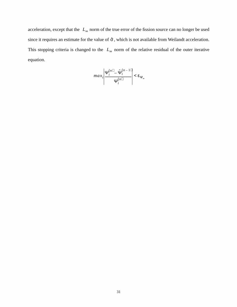
acceleration, except that the norm of the true error of the fission source can no longer b
since it requires an estimate for the value of , which is not available from Weilandt accelera
This stopping criteria is changed to the norm of the relative residual of the outer iter
equation.
L∞
σ
L∞
maxiΨi
n( ) Ψin 1–( )
–
Ψin( )---------------------------------- εΨ∞
<
31

32
II.3. Steady-State Fixed-Source Problem
Real reactors utilize fixed neutron sources to facilitate start-ups and assure high enough
count rates for nuclear instrumentation used for control and protection. We refer to the analysis of
this situation as a Fixed Source Problem [FSP]. Mathematically, the multi-group diffusion
equation for a steady-state FSP is as follows,
(46)
where dependence has been surpressed and denotes the external neutron source.
This equation can be solved utilizing nearly exactly the same method as utilized for the
AEVP, except now appears on the RHS in the NEM equations associated with the AEVP.
This applies to both the FDM equation and two-node problem equations. The biggest difference
in the solution of the FSP versus AEVP originates because the FSP does not involve determining
the fundamental eigenvector. This impacts the outer iterations of the FDM equations in the
following manner. For the AEVP, the rate of convergence of the Power Method is determined by
the dominance ratio of the outer iterative matrix, ; by contrast, for the FSP the rate of
convergence is determined by the spectral radius, , where note that, . The
implication for the Chebyshev Semi-Iterative method is whenever appeared in the
governing equations, it should be replaced by . The other implication for the Chebyshev
Semi-Iterative method is that the FSP versus AEVP outer iterations will converge much slower
since for problems of interest. When Weilandt Shift is employed,
neither of these issues appear. A special implementation of the Coarse Mesh Rebalance method,
as now described, is utilized for the FSP to accelerate convergence.
∇ Dg∇φg⋅– Σtgφg+ Σsgg′φg′g′ 1=
G
∑ χg νg′Σ fg′φg′ Sextg+
g′ 1=
G
∑+=
r Sextg
Sextg
σ Q( )
ρ Q( ) ρ Q( ) keff=
σ Q( )
ρ Q( )
σ Q( ) ρ Q( )< keff 1≈=
ith
erative
flux
e used
ingle
antly
imate
y in
c(q) is
hting
II.3.a. Fixed-Source Scaling Factor Method
When the FSP is near-critical (i.e. approaches unity), convergence rates w
Chebyshev acceleration are unacceptably slow. This convergence is slow even when the it
flux shape is correct but the magnitude is in error. To accelerate convergence of the
magnitude, a global coarse mesh rebalance [12] is proposed. This acceleration option can b
with when either Chebyshev or Weilandt Shift acceleration are employed. Application of a s
scaling prior to the start of a new Chebyshev acceleration cycle sometimes can signific
reduce the required number of outer iterations. This reduction is achieved by an approx
procedure that attempts to scale the current iterative flux vector to the exact flux vector.
For steady-state the FDM based matrix equation analogous to Eq. (27) is
(47)
Now assume that theqth outer iterative estimate of the flux has the correct shape but is off onl
magnitude by a factor of c(q) from the exact solution,i.e.
(48)
Then it follows that an improvedqth iterate is given by
(49)
or in terms of the fission source
(50)
where is the Chebyshev accelerated fission source. The fixed source scaling factor,
defined so as to preserve neutron balance in an integral sense. Utilizing Galarkin weig
defines c(q) as follows
(51)
ρ Q( )
A F–( )φ Sext=
φ cq( )φ
q( )=
φq( )
cq( )φ
q( )=
Ψq( )
cq( )Ψ
q( )=
Ψq( )
cq( ) φ
q( )Sext,⟨ ⟩
φq( )
A cq( )( ) F c
q( )( )–( )φq( )
,⟨ ⟩--------------------------------------------------------------------------=
33
sed in
inates
as a
l, the
be
er
ated as
51)
r
(51)
e.
noted
This method does differ from the fundamental mode contamination adjustment approach u
DIF3D [10].
The dependence on the scale factor of the matrix operators indicated in Eq. (51) orig
because of thermal-hydraulic (T-H) feedback, implying the solution of Eq. (51) for c(q) involves a
non-linear root search. Difficulty in this search originates because the Eq. (51) RHS h
singularity, which is addressed as follows. It is known that when the reactor is close to critica
flux can be approximated by the AEVP flux. This implies that the Eq. (51) RHS can
approximated as
(52)
where is the eigenvalue (i.e. ). Since the second bracketed term varies much slow
than the first bracketed term as c(q) varies for a near critical system, the second term is tre
constant. We next assume that varies linearly with c(q).
(53)
The values of and are obtained by explicitly evaluating the Eq. (
RHS for the two scale factor values and using the resulting values in Eqn. (52) to solve fo
values. Substituting Eq. (53) into Eq. (52), and using this equation as the RHS of Eq.
produces a quadratic equation in terms of c(q), with one root denoted being the desired valu
For a steady-state problem the following steps are completed to implement the just
procedure:
Step 1: Calculate 0th outer iterative operator estimates and , based upon
flux used in T-H feedback calculations and accounting for external parameters (e.g.control
rod position).
λ0 c q( )( )1 λ0 c q( )( )–----------------------------
φq( )
Sext,⟨ ⟩
φq( )
F cq( )( )φ
q( ),⟨ ⟩
---------------------------------------------≅
λ0 λ0 keff=
λ0 cq( )( )
λ0 cq( )( ) λ0 c1
q( )( )λ0 c2
q( )( ) λ0 c1q( )( )–
c2q( )
c1q( )
–( )--------------------------------------------- c
q( )c1
q( )–( )+=
λ0 c1q( )( ) λ0 c2
q( )( )
λ0
c3q( )
A0 F0 flux φ0( )
=
34
ting
and
.
by
r the
actors
ately
nd the
lues of
and
ction
Step 2: Solve the FSP iteratively for a fixed number of outer iterations .
Step 3:Set and calculate the following: operator estimates and by repea
Step 1 using flux = (Step 2) flux, Eqn. (51) RHS, and .
Step 4:Set = (Step 3 Eq. (51) RHS) and calculate the following: operator estimates
by repeating Step 1 using flux, Eq. (51) RHS, and
Step 5: Solve quadratic equation for and calculate operator estimates and
repeating Step 1 using flux.
This basic process is repeated every so many outer iterations as specified by user input.
The just noted method scales energy groups equally, thus it does not account fo
energy spectrum shift that occurs as a result of T-H feedback. This is important in water re
due to the dependance of moderating power on water density. This effect can be approxim
accounted for as follows: Assume that leakage can be approximated by a treatment a
Prompt Jump approximation can be used to estimate the flux energy spectrum shift. The va
are spatially dependent and obtained from the current estimate of the flux distribution
prior to the scale factor impact on cross-sections via T-H feedback (i.e. after Step 2). Specifically
for a two-group problem, suppressing spatial dependance notation, we obtain
(54)
Now an improved estimate for the flux ratio can be obtained as follows, where cross-se
values now reflect the scale factor via T-H feedback (i.e.during Steps 3-5).
(55)
q( )
c1q( )
1= A1 F1
λ0 c1q( )( )
c2q( )
A2
F2 flux c2q( )
Step 2×= λ0 c2q( )( )
c3q( )
A3 F3
flux c3q( )
Step 2×=
DgBg2
Bg2
B22 1
D2------
Σr1
φ1q( )
φ2q( )---------
Σa2–=
φ1
φ2-----
i
D2 ciq( )( )B2
2 Σa2 ciq( )( )+
Σr1 ciq( )( )
--------------------------------------------------------=
35
r the
thod
ation
This
when
.
his is
r than
f the
We are now free to set either to the Step 2 flux value, and using Eq. (55) solve fo
other group flux. NESTLE selects in its implementation and solves for . The above me
can be generalized to a multi-group formulation and is done so in the NESTLE implement
for the case G=4.
The scaling process can be very effective in obtaining the correct flux magnitude.
avoids a serious problem associated with FSP type problems, which is particularly troubling
the initial guess of the flux is higher than the converged value (i.e. approaches from above)
However, when the reactor is very close to critical, the scaling process may break down. T
because with high neutron multiplication, and are nearly equal and are much large
which implies that to get an accurate estimate of a very accurate estimate o
shape of is required.
φ1 or φ2
φ1 φ2
Aφ Fφ
Sext A F–( )φ
φ
36

not
ll align
15].
hin
delity
nd
le, to
under
caling
ous to
ed. The
II.4. Nodal Model - Hexagonal Geometry
II.4.a. Eigenvalue Problem
Utilization of NEM for Hexagonal (Hex) geometry introduces several complications
encountered for Cartesian geometry, originating because the surfaces of the Hex do not a
with the Cartesian axis. This can be seen in Figure 2.
R.D. Lawrence addressed these difficulties in implementing the Hex NEM option in DIF3D [
NESTLE through version 5.0.2 utilized this earlier work, adapting it for implementation wit
the context of the non-linear iterative method. However, this treatment has questionable fi
due to the coarseness of hexagonal nodes,e.g. cross section of a fuel assembly. Chao a
Tsoulfanidis [16] applied a conformal mapping, which transforms a hexagon into a rectang
the diffusion equation before the transverse integration. The Laplacian operator is invariant
the conformal mapping. Therefore, the diffusion equation remains unchanged except for s
factors which multiply the diffusion operator. The resulting transverse equations are analog
the ones for rectangular nodes when intranodal cross section spatial dependence is treat
1
3-------h
2
3-------h
v u
x
y
h
Figure 2: Hex geometry dimensions and axis orientation.
37

ping
the
ode is
conformal mapping approach has been verified by Chao and Shattila [17] and Knight,et.al. [18].
Starting with Version 5.0.3, Version 5 series of NESTLE have adapted the conformal map
approach for implementation within the non-linear iterative method. The derivation of
governing equations in the Hexagonal-Z geometry is presented in this section.
Consider the following three-dimensional, multigroup diffusion equation:
. (56)
Assume that the hexagonal node is in the complex plane and the rectangular n
in the complex plane as shown in Figure 3.
The transformed diffusion equation for nodel and energy groupg has the following form:
(57)
Dgx
2
2
∂
∂
y2
2
∂
∂
z2
2
∂
∂+ +
– ΣRg
χg
k------νΣ f g
–+
φg x y z, ,( )
Σsg' g→
χg
k------νΣ f g'
+ φg' x y z, ,( )
g' g≠
G
∑=
W u iv+=
Z x iy+=
F A(0,0) B(a/2,0)
F
A(0,-R)
B
E
D (0,R)
CE(-a/2,b) D C(a/2,b)
v
u
Figure 3: Conformal mapping of a hexagon to a rectangle.
Dgl
u2
2
∂
∂
v2
2
∂
∂
z2
2
∂
∂+ +
– ΣRg
l χg
k------νΣ f g
l–
g2
u v,( )+ φgl
u v z, ,( )
Σsg' g→
l χg
k------νΣ f g'
l+
g2
u v,( )φg'l
u v z, ,( )g' g≠
G
∑=
38

must
size
up
effect,
fusion
:
where is a mapping function associated with the mapping from (x,y) to (u,v) coordinates.
To preserve the total area under the mapping, the side length of the hexagon ( )
be related to the base (a) and height (b) of the rectangle by
and . (58)
Selecting thev-coordinate to span from 0 tob, the u-coordinate to span from-a/2 to a/2 (see
Figure 3), and thez-coordinate (note that the lower casez denotes the normal axial direction) to
span from -c/2 to c/2, we apply the transverse integration on Eq. (57) over thev- andz-coordinates
on nodel and define:
(59)
. (60)
to obtain the following transverse integrated equation:
. (61)
Since the radial node size,i.e. one hexagonal assembly, is larger than the radial node
normally used for western LWRs,i.e. one fourth of a fuel assembly, the treatment of the burn
gradient effect within a hexagonal assembly is necessary. To capture the burnup gradient
spatially dependent cross sections are introduced. The burnup gradient effect on the dif
coefficients is assumed to be negligible. The spatially dependent cross section is written as
g2
u v,( )
R h 3⁄=
a 1.82308R≅ b 1.42510R≅
φgul
u( ) 1bc------ φg
lu v z, ,( ) vd zd
c– 2⁄
c 2⁄
∫0
b
∫=
g2
u( )
1bc------ g
2u v,( )φg
lu v z, ,( ) vd zd
c– 2⁄
c 2⁄
∫0
b
∫
φgul
u( )----------------------------------------------------------------------------- 1
b--- g
2u v,( ) vd
0
b
∫≅=
Dgl
u2
2
∂
∂– ΣRg
l χg
k------νΣ f g
l–
g2
u( )+ φgul
u( )
Σsg' g→
l χg
k------νΣ f g'
l+
g2
u( )φg'ul
u( )g' g≠
G
∑– L– gul
u( )=
39

. (62)
btain
of Eq.
, (62)
where is the node flux-volume weighted average cross section. By substituting Eq
into Eq. (61) and collecting the spatially varying part on the right hand side of Eq. (61), we o
the following equation:
, (63)
where
. (64)
Details on how to calculate and are presented in Section II.4.b.
The one-dimensional transverse integrated flux that appears on the left hand side
(63) is approximated using the following expansion:
, (65)
where
. (66)
denote polynomials of ordern which are orthonormal on the interval with
weight , implying that
Σxguu( ) Σxg
⟨ ⟩ δΣxguu( )+=
Σxg⟨ ⟩
Dgl
u2
2
∂
∂– ΣRg
l⟨ ⟩
χg
k------ νΣ f g
l⟨ ⟩–
g2
u( )+ φgul
u( )
Σsg' g→
l⟨ ⟩
χg
k------ νΣ f g'
l⟨ ⟩+
g2
u( )φg'ul
u( )g' g≠
G
∑– Qgul
u( ) Lgul
u( )–=
Qgul
u( ) δΣRgu
lu( )
χg
k------δνΣ f gu
lu( )–
g2
u( )φgul
u( )=
δΣsg' gu→
lu( )
χg
k------δνΣ f g'u
lu( )+
g2
u( )φg'ul
u( )g' g≠
G
∑–
Σxg⟨ ⟩ δΣxgu
u( )
φgl
u( ) Agl
kglu( )cosh Bg
lkg
lu( )sinh ang
lWn u( )
n 0=
2
∑+ +=
kgl
g2
a 2⁄( ) ΣRg
l⟨ ⟩
χg
k------ νΣ f g
l⟨ ⟩– Dg
l⁄=
Wn u( ) a 2⁄– a 2⁄,[ ]
g2
u( )
40

l
es of
ients
n the
. (67)
The polynomials that satisfy these conditions are determined to be as follows:
, (68)
, (69)
and , (70)
where
. (71)
The mapping scale function, , is symmetric inu and is approximated by a polynomia
function:
. (72)
The polynomial coefficients are selected such that as required. The valu
taken from Ref. [16] and given in Table 2 are used to determine the expansion coeffic
of Eq. (72).
The leakage terms are directly expressible in terms of the surface currents i
1a--- g
2u( )Wm u( )Wn u( ) ud
a 2⁄–
a 2⁄
∫ δmn=
W0 u( ) κ0=
W1 u( ) κ1u=
W2 u( ) κ1
u2 κ0 κ1⁄( )2
–
κ1 κ2⁄( )2 κ0 κ1⁄( )2–
---------------------------------------------------------=
κn1
2a--- u
2ng
2u( ) ud
0
a 2⁄
∫
---------------------------------------------=
g2
u( )
g2
u( ) cnu
a 2⁄----------
n
n 0=
6
∑=
g2
u( ) ud0
a 2⁄∫ a
2---=
g2
u( )
cn
Table 2: Values ofg2(u) as a function ofu.
u/a/2 0.001 0.1 0.2 0.3 0.4 0.5 0.6 0.7 0.8 0.9 1.0
g2(u) 2.279 1.594 1.353 1.173 1.025 0.897 0.786 0.690 0.609 0.544 0.507
Lug
lu( )
41

e
e two
or each
gon is
transverse directions, which in terms of thez- andv-directed leakage is given by:
. (73)
The axial leakage component, , is assumed to be given by a simple parabola in :
, (74)
where thez-direction node-averaged leakage in nodel can be expressed in terms of surfac
average currents by
, (75)
and the expansion coefficients of Eq.(74) can be solved for in terms of and
so as to preserve the node-averaged leakages in nodel-1, l, andl+1 :
and . (76)
Thev-directed transverse leakage component is given by:
, (77)
where and are the profiles of the physical currents on the two top surfaces and th
bottom surfaces of the hexagon, respectively. The physical currents are known on average f
face of the hexagon. Assuming that the physical current on each surface of the hexa
constant, we can write
for and for . (78)
Lug
lu( ) Lug
z l,u( ) Lug
v l,u( )+=
Lug
zu
Lug
z l,u( ) Lug
z l,ρ1g
lf 1 u( ) ρ2g
lf 2 u( )+ +=
Lug
z l, 1∆z------ Jg z+,
z l,Jg z-,
z l,–( )=
ρig
l
Lug
z l 1–,Lug
z l 1+,
u
-3a/2 -a/2 a/2 3a/2
l-1 l l+1
ρ1g
lLug
z l 1+,Lug
z l 1–,–
4---------------------------------------------= ρ2g
lLug
z l 1+,Lug
z l 1–,+
12----------------------------------------------
Lug
z l,
6---------–=
Luv l,
u( ) 1b---g u 0,( ) JT u( ) JB u( )–[ ]=
JT JB
JT u( ) JTM= a 2⁄– u 0≤ ≤ JT u( ) JTP= 0 u a 2⁄≤ ≤
42

is
es of
iated
he
usly for
where the meaning of the surface-averaged current subscript notation is depicted below.
The surface current on the bottom surfaces of hexagon is defined in a similar manner.
The profile of the linear mapping scale function appearing in Eq. (77)
approximated using the following function:
. (79)
The values of taken from Ref. [16] and given in Table 3 are used to obtain the valu
and appearing in Eq. (72).
For the v-direction transverse integrated diffusion equation, the derivation and assoc
transverse leakage term treatment are nearly the same as done for theu-direction transverse
integrated diffusion equation. For thez-direction transverse integrated diffusion equation, t
derivation and associated transverse leakage term treatment are the same as done previo
Cartesian geometry.
JBPJBM
JTMJTP
g u 0,( )
g u 0,( ) 1 u–u
------------ 1 3⁄
γ1x γ0+( )≅
g u 0,( )
γo γ1
Table 3: Values ofg(u,0) as a function ofu.
u/a/2 0.001 0.1 0.2 0.3 0.4 0.5 0.6 0.7 0.8 0.9 1.0
g(u,0) 8.078 1.739 1.372 1.183 1.053 0.947 0.851 0.756 0.650 0.510 0.000
43

the
e
two-
omial
II.4.b. Intranodal Burnup Gradient Treatment
The two-dimensional intranodal cross section distribution is approximated using
following polynomial function:
, (80)
where:
.
Clearly the expansion coefficients of the polynomial have been selected to make th
coefficients equal to surface and node average cross-section values. Similarly, the
dimensional flux distribution within an assembly can also be represented by the same polyn
expansion:
, (81)
so it follows that the coefficients take on the surface and node average flux values.
Σxgx y,( ) Sng
Pn x y,( )n 1=
7
∑=
S1gΣxg
west... west surface average cross section,=
S2gΣxg
east... east surface average cross section,=
S3gΣxg
northwest... northwest surface average cross section,=
S4gΣxg
southeast... southeast surface average cross section,=
S5gΣxg
northeast... northeast surface average cross section,=
S6gΣxg
southwest... southwest surface average cross section,=
S7gΣxg
⟨ ⟩ ... node average cross section,=
Pn x y,( ) cmnx( )
xm
cmny( )
ym
+( )m 0=
2
∑ c3nxy c4nxy2
+ +=
Pn x y,( ) Sng
φg x y,( ) FngPn x y,( )
n 1=
7
∑=
Fng
44

ross
two-
n
t
flux-
an
Utilizing these polynomial expansions, the node flux-volume average value of the c
section, which is defined to preserve reaction rates, defined as
(82)
can be evaluated. Next, the following steps are performed in order to transform the
dimensional distribution in theZ-plane domain ( ) into a one-dimensional distributio
in one of the coordinates of theW-plane ( ). At the west ( ) and eas
( ) surfaces of the conformally-mapped rectangle, the transversely-integrated,
volume weighted cross section can be calculated as:
, (83)
where denotes a function which transforms a point at in theW-plane toy-
coordinate at in the Z-plane. The relationship between they- andv-coordinates is
shown in Figure 4. Note that the function is approximated by a polynomial function:
. (84)
Utilizing , , and values obtained from Eqs. (82) and (83), we c
approximate the profile of in Eq. (62) with a second-order polynomial function:
. (85)
Σxg⟨ ⟩
xdR 3–2
--------------
0
∫ ydx–
3------- R–
x
3------- R+
∫ Σxgx y,( )φg x y,( ) xd
0
R 32
-----------
∫ ydx
3------- R–
x–
3------- R+
∫ Σxgx y,( )φg x y,( )+
3 32
----------R2
φg⟨ ⟩
------------------------------------------------------------------------------------------------------------------------------------------------------------------------------------=
Z x iy+=
W u iv+= u a 2⁄–=
u a 2⁄=
Σxg
a2---±
Σxg
R 32
-----------± y, φg
R 32
-----------± y, g
a2---± f v y( ),
ydR 2⁄–
R 2⁄∫
bφga2---±
g2 a
2---±
--------------------------------------------------------------------------------------------------------------------------=
f v y( ) a 2⁄± v,( )
x R 3± 2⁄=
f v y( )
f v y( ) R cnyR---
n
n 0=
3
∑=
Σxga 2⁄–( ) Σxg
a 2⁄( ) Σxg⟨ ⟩
Σxgu( )
Σxgu( ) Σxg
⟨ ⟩ 12--- Σxg
a2---
Σxg
a2---–
– u
a 2⁄----------
+=
12--- Σxg
a2---
Σxg
a2---–
+ Σxg
⟨ ⟩–12---
3u
a 2⁄----------
21–
+
45

e
on:
into
).
Similarly, the one-dimensional flux distribution in theu-direction appearing in Eq. (64) can b
written as:
, (86)
where
. (87)
The mapping scale function at can also be approximated by a polynomial functi
. (88)
The fitted versus exact values of are shown in Figure 5. By substituting Eq. (84)
Eq. (88), we can determine the function which appears in Eqs. (83) and (87
φg u( ) φg⟨ ⟩ 12--- φg
a2---
φga2---–
– u
a 2⁄----------
+=
12--- φg
a2---
φga2---–
+ φg⟨ ⟩–
12---
3u
a 2⁄----------
21–
+
φga2---±
φg
R 32
-----------± y, g
a2---± f v y( ),
yd
R 2⁄–
R 2⁄
∫
bg2 a
2---±
-----------------------------------------------------------------------------------=
u a 2⁄±=
ga2---± v,
cnvb---
n
n 0=
6
∑=
g a 2⁄± v,( )
g a 2⁄± f v y( ),( )
46

Figure 4: v- vs.y-coordinates atx=R(30.5/2).
0
0.2
0.4
0.6
0.8
1
1.2
1.4
1.6
-0.6 -0.4 -0.2 0 0.2 0.4 0.6
v/R
y/R
data
fv(x,y)
Figure 5: Mapping scale function atu=a/2.
0
0.1
0.2
0.3
0.4
0.5
0.6
0.7
0.8
0.9
0 0.05 0.1 0.15 0.2 0.25 0.3 0.35 0.4 0.45 0.5
g(a
/2,v
)
v/b
data
fitted __
47

anner
ain the
cted
at the
23) is
e
plies
urface
oduces
hich is
nd to
er
II.4.c. Non-Linear Iterative Strategy
For Hexagonal-Z geometry, the non-linear iterative strategy is applied in the same m
as for Cartesian geometry. For each surface of a node, a two-node problem is solved to obt
NEM predicted surface-averaged current based upon the FDM flux solution utilizing corre
coupling coefficients. The corrected coupling coefficients are determined demanding th
FDM and NEM predicted currents agree. In the radial plane for Hexagonal geometry, Eq. (
modified to read as follows:
. (89)
The conformal mapping is used when formulating the two-node problem, with thu-
direction in theW-plane always selected as the direction transversing the two nodes. This im
that three two-node problems are solved for each node to obtain the three radial plane s
average currents associated with half of the hexagonal surfaces. The two-node problem pr
a 10G x 10G linear system of equations, where G denotes the number of energy groups, w
constructed by applying NEM relations to two adjoining nodes. The 10G unknowns correspo
the five coefficients in Eq. (65) x two nodes x G neutron energy groups. For simplicity, consid
two arbitrary conformally-mapped nodes in theu-direction and denote these nodes as nodel and
nodel+1 .
In order to solve the 10G unknowns, the following constraints are applied:
• Surface flux discontinuity on the interior surface.
• Surface current continuity on the interior surface.
Dgx +l FDM, 2Dg
lDg
l 1+
Dgl
Dgl 1+
+---------------------------=
nodel nodel+1u- u+
48

• The matching of the zeroth moment projection of the two sides of Eq. (63).
• The matching of the first moment projection of the two sides of Eq. (63).
• The matching of the second moment projection of the two sides of Eq. (63).
• Volume-averaged flux determined by the FDM solution.
Radial Directions (Example -u-direction):
Flux Discontinuity
(90)
Current Continuity
(91)
dgx+l
Agl kg
la
2---------
cosh Bgl kg
la
2---------
sinh a0g
l κ0
a1g
l κ1a
2------------------- a2g
l κ1
a2
4------
κ0
κ1------
2
–
κ1κ2------
2 κ0
κ1------
2
–
-----------------------------------------+ + + + =
dgx-l 1+
Agl 1+ kg
l 1+a
2-----------------
Bgl 1+ kg
l 1+a
2-----------------–
sinh a0g
l 1+ κ0 a1g
l 1+ κ1a2---– a2g
l 1+ κ1
a2
4------
κ0
κ1------
2
–
κ1κ2------
2 κ0
κ1------
2
–
-----------------------------------------+ +–cosh
Dgl
Agl
kgl kg
la
2---------
sinh Bgl
kgl kg
la
2---------
cosh a1g
l κ1
a2g
laκ1
κ1κ2------
2 κ0
κ1------
2
–
-----------------------------------------+ + +– =
Dgl 1+
A– gl 1+
kgl 1+ kg
l 1+a
2-----------------
sinh Bgl 1+
kgl 1+ kg
l 1+a
2-----------------
cosh a1gl 1+ κ1
a2g
laκ1
κ1κ2------
2 κ0
κ1------
2
–
-----------------------------------------–+ +
49

Zeroth Moment Balance
, (92)
where
, (93)
, (94)
, (95)
and . (96)
First Moment Balance
, (97)
where
, (98)
, (99)
, (100)
α0g
lAg
l ξ0la2g
l+ =
Q0g
lL0g
l– ΣRg
l⟨ ⟩
χg
k------ νΣ f g
l⟨ ⟩– φg
l⟨ ⟩– Σsg' g→
l⟨ ⟩
χg
k------ νΣ f g'
l⟨ ⟩+
φg'l⟨ ⟩
g' g≠
G
∑+
α0g
l2
κ0Dglkg
l
a------------------- kg
l a2---
sinh–=
ξ0g
l 2Dgl κ0κ1–
κ1 κ2⁄( )2 κ0 κ1⁄( )2–
---------------------------------------------------------=
Q0g
l 1a--- W0 u( )g2
u( )Qugu( ) ud
a 2⁄–
a 2⁄
∫=
L0g
lκ0 Lug
z l, 975817911---------------
JTP JTM JBP– JBM–+
b-----------------------------------------------------------+=
β1g
lBg
l β1gg'
lB
g'
l
g' g≠
G
∑ ζ1g
la1g
l ζ1gg'
la1g'
l
g' g≠
G
∑+ + + Q1g
lL1g
l–=
β1g
l κ1
2a------ 4Dg
lkg
l a2---
sinh 2Dglkg
la kg
l a2---
cosh– ΣR0g
l χg
k------νΣ f 0g
l–
snh1g
l+=
β1gg'
l Σsg' g→
l⟨ ⟩
χg
k------ νΣ f g'
l⟨ ⟩+
– snh1g'
l=
ζ1g
l ΣRg
l⟨ ⟩
χg
k------ νΣ f g
l⟨ ⟩–=
50

, (101)
, (102)
, (103)
and . (104)
Second Moment Balance
, (105)
where
, (106)
, (107)
, (108)
ζ1gg'
l Σsg' g→
l⟨ ⟩
χg
k------ νΣ f g'
l⟨ ⟩+
–=
Q1g
l 1a--- W1 u( )g2
u( )Qugu( ) ud
a 2⁄–
a 2⁄
∫=
L1g
lκ1a
ρ1g
l
6--------
67730697803------------------
JTP JTM– JBP– JBM+
b-----------------------------------------------------------+=
snh1g
l 1a--- W1 u( )g2
u( ) kglu( )sinh ud
a 2⁄–
a 2⁄
∫=
α2g
lAg
l α2gg'
lA
g'
l
g' g≠
G
∑ γ2g
la0g
l ξ0la2g
l ξ2gg'
la2g'
l
g' g≠
G
∑+ + + + Q2g
lL2g
l–=
α2g
l 1
4aκ1
κ1
κ2------
2 κ0
κ1------
2
–
---------------------------------------------------- 16Dgl κ1
2
kgl
------ kgl a2---
sinh– 8κ02Dg
lkg
l kgla
2--------
sinh+
=
aκ12
8Dgl
kgl a2---
cosh 2aDglkg
l kgla
2--------
sinh–+
ΣRg
l⟨ ⟩
χg
k------ νΣ f g
l⟨ ⟩–
csh2g
l+
α2gg'
l Σsg' g→
l⟨ ⟩
χg
k------ νΣ f g'
l⟨ ⟩+
csh2g'
l
g' g≠
G
∑–=
γ2g
l 1
4aκ1
κ1
κ2------
2 κ0
κ1------
2
–
---------------------------------------------------- 8Dgl κ1
2κ0a– Dgl 8aκ0
2κ1
κ1
κ2------
2 κ0
κ1------
2
–
--------------------------------------- aκ128Dg
l κ0+ +
=
51

, (109)
, (110)
, (111)
, (112)
and . (113)
Volume-averaged flux
(114)
where
(115)
ξ2g
l 1
4aκ1 κ1 κ2⁄( )2 κ0 κ1⁄( )2–
----------------------------------------------------------------------
8Dgl κ1
3a
a2
12------
κ0
κ1------
2
–
– Dgl
8aκ02κ1( )+
κ1 κ2⁄( )2 κ0 κ1⁄( )2–
-----------------------------------------------------------------------------------------------
=
aκ12 8Dg
l κ1 a 2⁄( )2 κ0 κ1⁄( )2–[ ] 2Dg
la
2κ1–
κ1 κ2⁄( )2 κ0 κ1⁄( )2–
--------------------------------------------------------------------------------------------------+
ΣRg
l⟨ ⟩
χg
k------ νΣ f g
l⟨ ⟩–
+
ξ2gg'
l Σsg' g→
l⟨ ⟩
χg
k------ νΣ f g'
l⟨ ⟩+
g' g≠
G
∑–=
Q2g
l 1a--- W2 u( )g2
u( )Qugu( ) ud
a 2⁄–
a 2⁄
∫=
L2g
l κ1a2
κ1 κ2⁄( )2 κ0 κ1⁄( )2–
---------------------------------------------------------Lug
z l,
12---------
ρ2g
l
30--------
4169149796------------------
JTP JTM JBP– JBM–+
b-----------------------------------------------------------+ +
=
κ1 κ0 κ1⁄( )2
κ1 κ2⁄( )2 κ0 κ1⁄( )2–
--------------------------------------------------------- Lug
z l, 975817911---------------
JTP JTM JBP– JBM–+
b-----------------------------------------------------------+
–
csh2g
l 1a--- W2 u( )g2
u( ) kglu( )cosh ud
a 2⁄–
a 2⁄
∫=
α3g
lAg
la0g
l+ φg⟨ ⟩ l FDM,
=
α3g
l 1a--- kg
lu( )cosh g
2u( ) ud
a 2⁄–a 2⁄∫=
52

wing
y. For
atrix
atrix
. For
ming
atrix
olved
lems,
22).
Axial Direction:
Flux Discontinuity
(116)
Current Continuity
(117)
Nodal Balance
(118)
First Moment
(119)
Second Moment
(120)
For the z-direction, the same matrix structure as for Cartesian geometry results allo
rearrangement of the associated two-node problem coefficient matrix to achieve reducibilit
the u-direction, the two-node problem for two groups can be reduced from a 20 X 20 m
problem to a 16 X 16 matrix problem by performing a Gaussian elimination. The 16 X 16 m
system can be further reduced to two 4 X 4 matrix problems and one 8 X 8 matrix problem
four groups the 40 X 40 matrix problem can be reduced to 32 X 32 matrix system by perfor
Gaussian elimination. The 32 X 32 matrix system can be further reduced to two 8 X 8 m
problems and one 16 X 16 matrix problem. The associated matrix problems are s
analytically to reduce floating point operations required. Having solved the two-node prob
the corrections to the coupling coefficients can be obtained as previously indicated in Eq. (
dgz+l
agz1l
agz2l
+[ ] dgz–l 1+
agz1l 1+
agz2l 1+
–[ ]+ 2 dgz–l 1+ φg
l 1+dgz+
l φgl
–[ ]=
Dgl
zl∆
------- agz1l
3agz2l 1
2---agz3
l 15---agz4
l+ + +
Dgl 1+
zl 1+∆
-------------- agz1l 1+
3agz2l 1+
–12---agz3
l 1+ 15---agz4
l 1+–+– 0=
Dgl
zl∆
-------
–1
zl∆
------- 6agz2
l 25---
agz4l
+2
3h------
Lgxl
Lgul
Lgvl
+ +( )– Agl φg
l– Qgg′
l φg′l
g′ g≠
G
∑+=
10 Aglagz1
lQgg′
lag′z1
l
g′ g≠
G
∑+– 60
zl∆
------- Dg
l
zl∆
-------
Agl
+ agz3l
Qgg′l
ag′z3l
g′ g≠
G
∑–+ 102
3h------
ρgxy1l
=
35 Aglagz2
lQgg′
lag′z2
l
g′ g≠
G
∑+– 140
zl∆
--------- Dg
l
zl∆
-------
Agl
+ agz4l
Qgg′l
ag′z4l
g′ g≠
G
∑–+ 352
3h------
ρgxy2l
=
53

limits
ction
ction
tion
arying
ithin
ttice
flux
the
erage
ik has
orage
where
n the
as for
II.4.d. Pin-power Reconstruction Method
Pin-power reconstruction is necessary when utilizing nodal methods so that thermal
can be verified. For NESTLE Hexagonal geometry, we have utilized a pin-power reconstru
method similar to the method developed by Chao and Shatilla [17]. The pin-power reconstru
method implemented in NESTLE is described below.
A common assumption of pin-power reconstruction methods is that the flux distribu
within a node can be represented as the product of a smooth intra-nodal flux and a highly v
flux based upon the lattice physics solution. The intra-nodal flux represents the smooth w
node spatial flux variation of the homogenized problem. It corrects for the fact that the la
physics calculations are completed with reflective boundary conditions. The highly varying
obtained from the lattice physics solution accounts for the pin cell heterogeneities within
lattice, under the condition of reflective boundary conditions. When normalized to a node av
flux of one, the highly varying flux function is referred to as a flux form factor.
We have also adopted the Studsvik approach with regards to the form factors. Studsv
elected to utilize a power versus flux form factor. This results in some computation and st
reductions. We can begin to mathematically state their method as follows for nodel, where node
dependence have been suppressed for clarity: The power at cylindrical coordinates ,
r=0 denotes the hexagonal node center, is determined using
(121)
where the power form factor is defined by
. (122)
The power form factors, on a unit cell average basis, are input into NESTLE based upo
lattice physic code’s predictions. Control rod insertion dependence is treated the same
r θ,( )
p r θ,( ) pIntra
r θ,( ) FF r θ,( )×=
FF r θ,( ) pLattice
r θ,( )
p⟨ ⟩Lattice---------------------------------=
54
ing as
the
intra-
to a
oup-
er
alues
tions is
ion
cross-sections; that is, the unrodded and rodded power form factors are combined us
weights the axial fraction of the node unrodded and rodded, respectively.
The intra-nodal power is obtained from the intra-nodal group fluxes via
(123)
As used in Eq. (121), the value of is evaluated at a pin’s center and multiplied by
unit cell average basis power form factor for that pin to obtain the pin power. To evaluate the
nodal power using Eq. (123) one must evaluate the intra-nodal flux and cross-section.
The pin-power reconstruction option in the current version of NESTLE is restricted
two neutron energy group problem (NG=2) due to the complication in determining the gr
wise intra-nodal fluxes for NG > 2. For a NESTLE problem with NG > 2, the pin-pow
reconstruction is performed by group collapsing the flux and macroscopic cross section v
into two-group fluxes and cross sections as shown in Eqs. 124 through 126.
(124)
(125)
(126)
The pin-power reconstruction methodology based upon the two-group fluxes and cross sec
detailed below.
To obtain the intra-nodal flux, we start by writing the two-group neutron diffus
equation over a homogeneous hexagonal node in the following form:
, (127)
pIntra
r θ,( ) κgΣ fgIntra
r θ,( )g 1=
G
∑= φgIntra
r θ,( )
pIntra
r θ,( )
φGcollapsed φg
g G∈∑=
ΣxG
collapsed Σxgφg
g G∈∑ φg
g G∈∑⁄=
ΣsG G''→
collapsed Σxg g'→φg
g G∈∑
g' G'∈∑
φgg G∈∑⁄=
∇2φ Bφ– 0=
55

to
Eq.
to
where and . We can cast this matrix equation in
diagonal form by first defining
, (128)
where are the eigenvectors of . Now, let which allows us to rewrite
(127) as:
. (129)
Substitute and into Eq. (129) and denote and
obtain:
. (130)
The solution to Eq. (130) in cylindrical coordinates can be shown to be given by
(131)
and
B
ΣR1νΣ f 1
–( )
D1--------------------------------
ν– Σ f 2
D1---------------
Σs12
D2-----------–
Σa2
D2--------
= φφ1
φ2
=
P ψ1 ψ2≡
ψ11 ψ12
ψ21 ψ22
=
ψi Bψi λiψi= φ PΦ=
∇2Φ
λ1 0
0 λ2
Φ– 0=
µ2 λ1–= ν2 λ2= Φ1 Φµ= Φ1 Φν=
∇2 Φµ
Φν
µ20
0 ν–2
Φµ
Φν+ 0=
Φµ r θ,( ) Aµ α( ) µr θ α–( )cos( )sin Bµ α( ) µr θ α–( )cos( )cos+[ ] αd
0
2π
∫=
Cµ α( ) µr θ α–( )sin( )cos Dµ α( ) µr θ α–( )sin( )sin+[ ] αd
0
2π
∫+
56

We
need
e 12
d
of the
nomial
e
t flux
each
t three
orner
d are
by a
e the
d the
s shown
, (132)
where , , , and are direction-dependent superposition coefficients.
numerically perform the integration operations shown in Eqs. (131) and (132), implying we
to determine the values of , , , and at discrete values of . There ar
known values that can be utilized as constraints,i.e. six homogeneous corner point flux values an
six homogeneous surface average flux values. For simplicity, we assumed that the profile
surface average flux on a hexagonal surface can be approximated by a quadratic poly
where . Two corner point flux values and th
surface average flux value are imposed as constraints to determinec0, c1, andc2 coefficients. We
can then determine the flux value at the center of the hexagonal surface ( ). The poin
values at the center of the six hexagonal along with the six corner point flux values for
energy group can be imposed as constraints to evaluate the superposition coefficients a
values of .
The surface average fluxes are readily available from the nodal solution while the c
point flux values are not. The corner point flux values for the pin-power reconstruction metho
obtained in the following manner. First the flux in the vicinity of a corner point is represented
polynomial function in (x,y), with the associated expansion coefficients fitted so as to preserv
node volume-averaged fluxes of the three nodes surrounding the corner point an
heterogeneous surface average fluxes on the three interfaces meeting at the corner point, a
in Figure 6.
Φν r θ,( ) Aν α( ) νr θ α–( )cos( )sinh Bν α( ) νr θ α–( )cos( )cosh+[ ] αd
0
2π
∫=
Cν α( ) νr θ α–( )sin( )cosh Dν α( ) νr θ α–( )sin( )sinh+[ ] αd
0
2π
∫+
A α( ) B α( ) C α( ) D α( )
A α( ) B α( ) C α( ) D α( ) α
φgsurface
s( ) c0 c1s c2s2
+ += s R– 2⁄ R 2⁄,[ ]∈
s 0=
α
57

ven
r
e
int flux
ysics
cross
de and
ective
n as a
The polynomial function used to approximate the flux in the vicinity of the corner point is gi
by
. (133)
Selecting a coordinate system such that (x,y)= corresponds to the location of the corne
point of interest, the corner point flux is simply given by . Th
resulting heterogeneous flux is continuous at a corner point. The homogeneous corner po
is then defined as:
(134)
The corner point ADF values that appear on the RHS are obtained from the lattice ph
calculation. This process is repeated for the other five corner points of nodel, providing all the
constraints required to solve for the expansion coefficients of the intra-nodal flux.
To evaluate the intra-nodal power distribution, the cross-section spatial variation a
the node must also be determined. This variation is associated with the homogenous no
corrects for the burnup distribution error made in the lattice physics code because refl
boundary conditions are assumed. This is accomplished by expanding the cross-sectio
Figure 6: Corner Flux Configuration.
node 1
node 2 node 3
s1 s2
s3
y
x
φg x y,( ) c0gc1g
x c2gy c3g
x2
c4gy
2c5g
xy+ + + + +=
0 0,( )
φgcorner( )Het φg 0 0,( ) c0g
= =
φgcorner( )Hom
φgcorner( )Het
ADFgcorner
----------------------------=
58
is
the
f the
seven
cross-
model
he node
s. The
uate
flux is
at even
s, the
s since
In all
surface
ers,
lue of
35)
tain
s are
polynomial inr andθ according to
, (135)
where and . The base of the polar coordinates
from the center of the hexagon to the center of the east surface.
Eq. (135) has eight unknown coefficients. Note that when solving for , one of
coefficients can be chosen arbitrarily because of a lack of linear independence o
expansion defined by Eq. (135). This implies that only seven constraints are required. The
constraints are obtained by demanding that the node and six surface average values of the
section be preserved. The cross-section values are obtained for the macroscopic depletion
based upon the node and surface average burnups. For the microscopic depletion model, t
and surface average burnups and isotopics are used to obtain the cross-section value
implication is that with pin-power reconstruction, the depletion calculation must now eval
surface average quantities based upon the homogenous flux. Since the homogenous
discontinuous across surfaces, the burnup and isotopics will also be discontinuous. Note th
though the user may elect to only do pin-power reconstruction on the highest power node
depletion calculation for surface average quantities must be completed on all node surface
the location of the highest power nodes under various core conditions is not known a priori.
cases, the node average thermal-hydraulic conditions are used to correct the node and
average cross-sections.
The last calculation that remains to be completed is the determination of pin-pow
which proceeds as follows. Eqs. (131) and (132) are evaluated at the fuel pin center va
for each fuel pin within the node to obtain the axially dependent fuel pin fluxes. Eq. (1
is also evaluated at the fuel pin center value of for each fuel pin within the node to ob
the axially dependent fuel pin cross-sections. When the group dependent flux value
κΣ f g
lr θ,( ) C0g
lC1ng
l γnn 1=
3
∑ C2ng
l γn2
n 1=
3
∑ C3gl γ1
3– γ2
3 γ33
–+( )+ + +=
γn r θ αn–( )cos= αn n 1–( ) π 3⁄( )= r θ,( )
C1n
C1n
r θ,( )
r θ,( )
59

xially
l pin
alize
at the
m
er
ting
in the
dial
multiplied by the cross-section values and summed over energy groups, the intra-nodal a
dependent fuel pin power is obtained. This quantity is multiplied by the axially dependent fue
power form factor to obtain the unnormalized axially dependent fuel pin power. To norm
these results, it is demanded that the axially dependent fuel pin relative powers be such th
associated node power is preserved, implying
(136)
In this expression,l denotes the node dependence andn denotes the fuel pin dependence. Fro
the values, the total peaking factor FQ value is determined assuming a flat axial pow
distribution within the node and determining the maximum value over alln. Having the axially
dependent fuel pin power distribution, the total fuel pin power is obtained by axially integra
those values associated with a specific pin and dividing by the active fuel pin length to obta
pin-wise radial power distribution. This information allows the determination of the ra
peaking factor , which completes the pin-power reconstruction calculations.
pnl
rn θn,( )∆vnl
n 1=
total number of fuel pins in a node
∑ plV
l=
pnl
rn θn,( )
F∆H
60

tron
source
up g
) and
. The
f the
utrons,
poral
II.5. Transient Problem
Under transient conditions, both the multi-group diffusion equation and delayed neu
precursor equations must be solved. These equations, accounting for an external neutron
and utilizing six precursor groups, are given by (suppressing andt dependences for clarity):
(137)
and
(138)
where the notation is identical as before except as now noted.
= neutron speed for energy group g
= fraction of prompt neutrons born into energy group g
= fraction of delayed neutrons for precursor group i born into energy gro
= neutron precursor concentration in precursor group i
= decay constant for precursor group i
= fraction of all fission neutrons emitted per fission in precursor group i
= total fraction of fission neutrons which are delayed
Alternately, the ‘eigenvalue initiated’ transient equations can be obtained from Eqs. (137
(138) by setting and by replacing with everywhere.
The neutron kinetics equations, Eqs. (137) and (138), involve differentials in space and time
time dependence is a difficult problem to treat in neutronics modeling due to the stiffness o
associated equations. The time constants range from very small, associated with prompt ne
to very long, associated with the longer lived precursors. NESTLE numerically treats the tem
r
1vg-----
t∂∂φg Σsgg′
φg′ 1 β–( )χgP( ) νg′Σ fg′φg′ χgi
D( )λiCi ∇ Dg⋅ ∇φg Σtgφg– Sextg++
i 1=
ID( )
∑+g′ 1=
G
∑+g′ 1=
G
∑=
t∂∂Ci βi νgΣ fgφg λiCi–
g 1=
G
∑= for i 1,...,ID( )
=
vg
χgP( )
χgiD( )
Ci
λi
βi
β
Sextg0= νgΣ fg νgΣ fg( ) k⁄
61
ology
crete
nce.
nd will
f the
[tn,
must
rator
early
dependence in a manner that results in a FSP, which can be solved utilizing the method
developed for the steady-state FSP.
The first step in this conversion to a FSP is to discretize the time domain into dis
times tnand to approximate the time derivative of the flux at time tn+l by a backward differe
(139)
This assures unconditional stability. Do note that spatial dependance notation has been a
continue to be suppressed in the equations.
To develop an expression for the precursors’ concentrations at time tn+1 in terms o
flux , Eq. (138) is solved utilizing the Integrating Factor method over time span
tn+1] to obtain
. (140)
To solve the above integral, a functional form for the time dependent neutron fission source
be assumed over time span [tn, tn+1]. Consistent with the backward difference ope
approximation for the time derivative of the flux, the fission source is assumed to vary lin
between time-steps,
(141)
Incorporating this approximation into Eq. (140) and rearranging terms, we obtain
, (142)
where
t∂∂φg
tn 1+
φg tn 1+( ) φg tn( )–
tn∆-------------------------------------------=
φg tn 1+( )
Ci tn 1+( ) Ci tn( )eλi tn∆–
βi υgΣ fgφg t′( )eλi tn 1+ t′–( )–
dt′g 1=
G
∑tn
tn 1+
∫+=
vgΣ fgφg t( ) vgΣ fgφg tn( )vgΣ fgφg tn 1+( ) vgΣ fgφg tn( )–
tn∆----------------------------------------------------------------------- t tn–( )+=
Ci tn 1+( ) Ci tn( )eλi tn∆–
Fin
0 νgΣ fgφg tn( ) Fin
1 νgΣ fgφg tn 1+( )g 1=
G
∑+g 1=
G
∑+=
62

) as the
of the
ould be
outer
.
fluxes,
e
dent
ents.
o-
(143)
and
(144)
Now substituting Eqs. (139) and (142) into Eq. (137) one obtains
(145)
where
(146)
In Eq. (145) all cross-sections are evaluated at time tn+1. Inspection of Eq. (145) indicates it to be
a FSP, with modified operators and source from the steady-state FSP. We refer to Eq. (145
transient FSP. Hence the application of NEM to the transient FSP and the iterative solution
resulting coupled equations can proceed exactly the same as for the steady-state FSP. As w
expected, the values of flux and adjusted FDM coupling coefficients at time for the 0th
iterative step are based upon their values at time tn.
If we proceed in this manner, in the two-node problems spatial moments of
would appear. As Eq. (146) indicates, is dependent upon and
The implication is that the expansion coefficients associated with the transverse integrated
obtained from solution of the two-node problems, at the previous time tn must be saved. The sam
is true for the precursor concentrations, which are treated like the flux for time depen
problems solved by NEM. This would substantially increase the computer memory requirem
To overcome this difficulty, further approximations are required in formulating the tw
Fin
1 βi
λi tn∆------------- tn∆ 1
λi---- 1 e
λi tn∆––( )–=
Fin
0F– i n
1 βi
λi---- 1 e
λi tn∆––( )+=
1tnνg∆
--------------φg tn 1+( ) ∇ D⋅ g∇φg tn 1+( ) Σtgφg tn 1+( )+– Σsgg′φg′ tn 1+( )
g′ 1=
G
∑=
1 β–( )χgP( ) χgi
D( )λiFin
1
i 1=
ID( )
∑+
+ vg′Σ fg′φg′ tn 1+( ) Sef fgtn 1+( )+
g′ 1=
G
∑
Sef fgtn 1+( ) χgi
D( )λiFin
0vg′Σ fg′φg′ tn( ) χgi
D( )λiCi tn( )eλi tn∆–
i 1=
ID( )
∑+g′ 1=
G
∑i 1=
ID( )
∑ 1tnvg∆
-------------φg tn( ) Sextgtn 1+( )+ +=
tn 1+
Sef fgtn 1+( )
Sef fgtn 1+( ) φg tn( ) Ci tn( )
63

is
hat the
ions of
pact
TLE
that is,
e flux
ues are
uted.
fferent
nd the
is that
sient
tate
5) and
node problems. Recognizing that the within node spatial dependence of
associated with the contributions from the delay neutrons and the external neutron source, t
external neutron source is assumed to be constant within a node, and that these contribut
neutrons are small, one would expect within node spatial shape to have little im
on the solution. This justifies treating spatial dependence approximately. In NES
this approximate treatment is done in the same manner as for the transverse leakages;
using a quadratic polynomial as indicated in Eq. (12). Now only node average values of th
and precursor concentrations at time must be saved. The node average precursor val
solved for via back substitution using Eq. (142) after the node average flux has been comp
This implementation does create one problem that must be addressed. Since di
spatial treatments are used at times and , the solution of the steady-state FSP a
transient FSP, now for steady-state conditions, will not agree. The practical consequence
when one utilizes the steady-state FSP solution to determine initial conditions for the tran
FSP, the flux will undergo a very mild transient with time even when the initial steady-s
conditions are preserved. This annoyance can be avoided by regrouping terms in Eqns. (14
(146) as follows.
(147)
where
(148)
(149)
Sef fgtn 1+( )
Sef fgtn 1+( )
Sef fgtn 1+( )
tn
tn tn 1+
∇ Dg∇φg tn 1+( ) Σtgφg tn 1+( )+⋅– =
Σsgg′φg′ tn 1+( ) χg νg′Σ fg′φg′ tn 1+( ) Sef fgtn 1+( )+
g′ 1=
G
∑+g′ 1=
G
∑
χg 1 β–( )χgP( ) βiχgi
D( )
i 1=
ID( )
∑+=
Sef fgtn 1+( ) χgi
D( ) λiFin
1 βi–( )i 1=
I D( )
∑
νg′Σ fg′φg′ tn 1+( )g′ 1=
G
∑=
1tnvg∆
-------------φg tn 1+( )– Sef fgtn 1+( )+
64

f
e all
that
eated
verse
ce the
nted in
e
in the
g the
iterative
node
ents
sure
sient
eby
ence,
flux.
Eq. (147) is recognized to be identical to the steady-state FSP except for the replacement o
with the modified effective source . Under steady-state conditions, equals sinc
the additional terms in Eq. (149) cancel. This is true even for the moments of
appear in the two-node problems provided the within node spatial dependence is tr
consistently for the variables appearing in Eq. (149) at times tn and tn+1; in particular, when they
are all treated by a quadratic polynomial as previously indicated by Eq. (12) for the trans
leakages. The implication is that the transient FSP under steady-state conditions will produ
same solution as produced by the steady-state FSP. This approach has been impleme
NESTLE.
Since the values of node average flux at time tn+1, the unknowns, now appear in th
modified effective source, an iterative approach is required. This is easily accomplished with
context of the non-linear iterative method of solving the NEM equations. Recall when solvin
two-node problems, node average fluxes are assumed known based upon the latest outer
values available for the FDM equation’s solution. For transient problems, this corresponds to
averaged flux values at time tn+1, which are precisely the values requires to evaluate the mom
of that appear in the two-node problems. This approach is utilized within NESTLE to as
the steady-state FSP solution does not “drift” when used as an initial condition in the tran
FSP.
To improve upon the initial iterative estimate of the fission source and flux, ther
hopefully minimizing the number of outer and inner iterations required to achieve converg
the 0th outer iterative estimates of both are determined utilizing a time extrapolated
Specifically, assuming an exponential time dependence, the0th iterative flux at time stepn+1 is
given by
(150)
Sextg
Sef fgSef fg
Sextg
Sef fgtn 1+( )
Sef fg
φg tn 1+( ) φg tn( )eωgn
∆tn
= whereωgn
1∆tn 1–--------------- ln
φg tn( )φg tn 1–( )---------------------
=
65

lue
n the
n be
ns, the
the
their
ux is
flux.
metric
n. The
sulting
attering
s (
rmal
oint
ients
ng not
ed flux
ethod
. To
is
EM
II.6. Adjoint Problem
The adjoint solution to the few-group neutron diffusion equation for the eigenva
problem is of interest. This follows since the adjoint flux can be used to estimate the effect o
reactivity of perturbations via the Raleigh quotient, derived from perturbation theory; and, ca
used to estimate kinetics parameters utilizing point-reactor kinetics theory. For these reaso
ability to solve for the adjoint flux of the eigenvalue problem has been incorporated into
NESTLE code.
For the FDM solution, the development of the equations that need to be solved and
solution are straight forward. The matrix system that needs to be solved for the adjoint fl
obtained by transposing the matrices of the matrix system that is solved for the ‘forward’
Since the matrices on a per energy group basis are symmetric in space, the only non-sym
components occur because of energy group coupling originating from scattering and fissio
transpose of the matrices associated with fission and scattering are easily taken and the re
matrix system solved. Since down-scatter now becomes up-scatter for the transposed sc
operator, one solves the few-group diffusion equation by sweeping from low to high energiei.e.
from high energy group number to low energy group number) in the outer iterations. The
scattering iterations are completed if up-scatter exists in the ‘forward’ problem.
For the NEM solution, the situation is more complicated. Mathematically the adj
solution we seek should not only include the group fluxes but also all the expansion coeffic
for the transverse integrated fluxes. This implies that the matrices we should be transposi
only correspond to the nodal balance equations, but also include all the transverse integrat
constraint equations. These matrices never really appear in the nonlinear NEM iterative m
like they would in a more traditional surface current response NEM solution methodology
overcome this incompatibility and to greatly simplify the adjoint flux solution for the NEM, it
assumed that the diffusion coupling correction coefficients that originate in the nonlinear N
66
ient to
ations
Since
sion
lving
ing the
flux
r the
ction
hese
non-
ses no
ndent
the
rmal-
ined
eeds
atically
the
roup.
e, the
iterative method do not change when the core is perturbed. When using the Raleigh quot
estimate reactivity changes due to core perturbations, this implies that the resulting perturb
to the matrix operators do not include perturbations to the coupling correction coefficients.
the coupling correction coefficients can be thought of as corrections to the normal FDM diffu
coupling coefficients, this approximation should be acceptable for many applications invo
estimating core reactivity.
Having made the above assumption, one need no longer be concerned with evaluat
adjoint, transverse integrated flux expansion coefficients, since they only couple to the
solution through the coupling correction coefficients. Therefore, to obtain the adjoint flux fo
NEM one follows exactly the same procedure as for the FDM, except that the coupling corre
coefficients determine by the ‘forward’ solution appear in the matrix operator. Since t
coupling correction coefficients make the spatial originated component of the matrices
symmetric, this must be treated in addition to the non-symmetry in energy groups. This cau
practical problems within NESTLE, where now the transpose of the energy group depe
matrices that appear in the inner iterations are utilized.
A final point needing discussion in regard to solving for the adjoint flux concerns
treatment of cross-section feedback corrections. In NESTLE all feedback effects due to the
hydraulics and the transient fission products are frozen at their ‘forward’ solution determ
values. This implies that before an adjoint solution can be completed, a ‘forward’ solution n
to be completed to obtain the feedback corrected cross-section values. This is done autom
by NESTLE when the adjoint solution option is selected.
To facilitate subsequent utilization of the adjoint flux solution, NESTLE contains
option to write out to a user specified file its values as a function of spatial node and energy g
In this manner other computer codes can utilize this file as input to evaluate, for exampl
core’s reactivity response to perturbations employing the Raleigh quotient.
67

del.
uation
olor
sity,
only
When
irectly
nsities
single
educed
odels,
f the
color,
olant
llows
p g
II.7. Cross-Section Model
NESTLE has the option of utilizing a macroscopic or microscopic cross-section mo
The macroscopic model determines the macroscopic cross-sections used in the diffusion eq
solver by characterizing them as a function of the following: node burnup; color (where c
refers to the initial composition of the material within the node), rod in or out, coolant den
coolant temperature, effective fuel temperature, and soluble poison concentration. The
isotopic number densities calculated are for the I-Xe and Pm-Sm transient fission products.
used in conjunction with microscopic cross-sections, these isotopes’ effects can be d
accounted for. The microscopic cross-section model also determines the isotopic number de
for the U234-U236 and U238-Pu242 fuel chains, two lumped fission product groups, and a
isotope depletable burnable poison. The relative advantages of both approaches are r
computational resources and increased accuracy for the macroscopic and microscopic m
respectively. We now discuss the macroscopic model, to be followed by a discussion o
microscopic model.
II.7.a. Macroscopic Model
The macroscopic model represents macroscopic cross-section for a given fuel
burnup and rod insertion as a Taylor series expansion in terms of coolant density, co
temperature, effective fuel temperature and soluble poison number density as fo
(suppressing fuel color, burnup and rod insertion notation):
(151)
where
= macroscopic cross-section for reaction type x and energy grou
without transient fission products corrected to local conditions
Σxg a1xga n 1+( )xg
n 1=
2
∑ ρ∆ c( )na4xg
Tc∆ a5xgTFeff
∆ a n 5+( )xg
n 1=
3
∑ N∆ sp( )n+ + + +=
Σxg
68

m
m
(PPM)
or of
atial
, one
cally
uces
tion
= expansion coefficients
= change in coolant density (g/cm3) from reference condition
= change in coolant temperature (˚F) from reference condition
= charge in square root of effective fuel temperature (˚F) fro
reference condition
= change in soluble poison number density (cm-3 x 10-24) fro
reference condition.
The soluble poison number density change accounts for both soluble poison concentration
and coolant density (ρc) changes. The effective fuel temperature is evaluated by
(152)
where
Wp = pellet weighting factor, which accounts for resonance flux depression in the interi
the pellet
Wc = core statistical weighting factor, that compensates for the lack of detail in the sp
description of the core
= volume average fuel pellet temperature (oF)
= surface average fuel pellet temperature (oF).
To obtain the macroscopic cross-section for node l free of transient fission products
employs Eq. (151) using the expansion coefficients for the fuel color of node l quadrati
interpolated to the node l burnup, accounting for control rod effects as follows
(153)
where is the fraction of node l rodded. This treatment, for coarse axial meshing, prod
the artificial behavior of control rod “cusping” when plotting integral rod worth versus inser
ajxg
ρc∆ ρc ρc0( )
–=
TC∆ TC TC0( )
–=
TFeff∆ TFeff
TFeff
0( )–=
Nsp∆ Nsp Nsp0( )
–=
TFeffTC WC WpTF 1 Wp–( )TFSrf
TC–+[ ]+=
TF
TFSrf
Σxgl
1 f Roddedl
–( ) Σxgl
( )Unrodded f Roddedl Σxg
l( )Rodded+=
f Roddedl
69
ction
d Sm
manner
ions for
ium
sient
es are
time-
spatial
depth. Finally correcting for the transient fission products’ effect on the absorption cross-se
we obtain
(154)
where,
with and denoting the Xe135 and Sm135 number densities for node l. The Xe an
microscopic absorption cross-sections are represented and evaluated in exactly the same
as the macroscopic cross-sections. As implied by the above equations, the reference condit
the macroscopic cross-section input are xenon and samarium free.
The following options exist in NESTLE in regard to establishing xenon and samar
number densities: equilibrium, transient, no xenon nor samarium, no xenon and tran
samarium, and frozen at restart values. When the option requires, the number densiti
determined by solving the I135-Xe135 and Pm149-Sm149 chain depletion equations. The
dependent depletion equations for the iodine-xenon chain are given by (again suppressing
dependence)
(155)
(156)
where subscripts I and Xe denote I135 and Xe135, respectively, and
= nuclei number density of isotope i
Σagl Σag
l ΣXeag
l∆ ΣSmag
l∆+ +=
ΣXeag
l∆ σXeag
lNXe
l=
ΣSmag
l∆ σSmag
lNSm
l=
NXel
NSml
tdd
NIl
t( ) γ Il Σ f g
lt( )φg
lt( )
g 1=
G
∑ λIlNI
lt( )–=
tdd
NXel
t( ) λI NIl
t( ) γ Xel Σ f g
lt( )φg
lt( )
g 1=
G
∑ λXeNXel
t( )–+=
σXeag
lt( )φg
lt( )NXe
lt( )
g 1=
G
∑–
Nil
t( )
70

dy-state
= microscopic absorption cross section of isotope i
= macroscopic fission cross section
= node average flux
= effective yield (atoms/fission) of isotope i
= decay constant of isotope i
Likewise, the depletion equations for the Promethium-Samarium chain are given by
(157)
(158)
where subscripts Pm and Sm denote Pm149 and Sm149, respectively. The pseudo stea
solutions of Eq. (155) through (158) are given by
(159)
(160)
for the Iodine-Xenon depletion chain and,
(161)
(162)
σi ag
lt( )
Σ f gt( )
φgl
t( )
γ il
λi
tdd
NPml
t( ) γPml Σ f g
lt( )φg
lt( )
g 1=
G
∑ λPmNPml
t( )–=
tdd
NSml
t( ) λPmNPml
t( ) σSmag
lt( )φg
lt( )NSm
lt( )
g 1=
G
∑–=
NI ∞
l
γ Il Σ f g
l
g 1=
G
∑ φgl
λI-----------------------------=
NXe∞
l
λI NI ∞
l γ Xel Σ f g
l
g 1=
G
∑ φgl
+
λXe σXeag
l
g 1=
G
∑ φgl
+
------------------------------------------------------=
NPm∞l
γPml Σ fg
l
g 1=
G
∑ φgl
λPm----------------------------------=
NSm∞
l λPmNPm∞l
σSmag
l
g 1=
G
∑ φgl
-----------------------------=
71

ber
s and
multi-
l, it is
inetics
ber
s, and
cross-
for the Promethium-Samarium depletion chain. Note that the equilibrium isotopic num
densities and flux are coupled. This is addressed by updating the number densitie
subsequently cross-sections during the outer iteration process associated with solving the
group diffusion equation for either the eigenvalue problem or steady-state FSP.
For the transient solutions, forward differencing over the time-step produces
(163)
(164)
(165)
(166)
where is the time-step associated with transient fission product conditions. In genera
selected smaller and larger than the time-steps used in the core depletion and neutron k
solutions, respectively.
II.7.b. Microscopic Model
The microscopic model only differs from the macroscopic model in that the num
densities of the U234-U236 and U238-Pu242 fuel chains, two lumped fission product group
a simple burnable poison are explicitly calculated and used to determine the macroscopic
sections. This implies that the macroscopic cross-section for node l is determined from
NIl
t t∆+( ) NIl
t( ) t γ Il Σ f g
l
g 1=
G
∑ t( )φgl
t( ) λI NIl
t( )–∆+=
NXel
t t∆+( ) NXel
t( ) t γ Xel Σ f g
l
g 1=
G
∑ t( )φgl
t( ) λI NIl
t( )+∆+=
λXeNXel
t( ) σXeag
lt( )φg
lt( )NXe
lt( )
g 1=
G
∑––
NPml
t t∆+( ) NPml
t( ) t∆ γPml Σ f g
lt( )φgl
t( ) λPmNPml
t( )–g 1=
G
∑+=
NSml
t t∆+( ) NSml
t( ) t∆ λPmNPml
t( ) σSmag
lt( )φg
lt( )NSm
lt( )
g 1=
G
∑–+=
t∆
72
n (
mple
67) are
rnup
l is
otopic
s
upon
g the
(167)
where
= macroscopic cross-section for the background (Bk) isotopes (i.e. without isotopes in set
)
=set of fissile and fertile isotopes, lumped fission products and simple burnable poisoi.e.
U234-U236 and U238-Pu242 chains, two lumped fission product groups, and si
burnable poison)
As before, the macroscopic and microscopic cross-sections appearing on the RHS of Eq.(1
determined by interpolating expansion coefficients for the fuel color of node l to the node l bu
and using the results in Eq. (151).
The computational effort associated with the microscopic cross-section mode
associated with evaluating node dependent microscopic cross-sections and solving the is
depletion equations, which can be expressed for the fuel isotopes in general form as follow
(168)
where
Do note that Plutonium isotopic production is assumed to occur instantaneously
neutron capture. Eq. (168) is solved utilizing the Integrating Factor Technique, assumin
Σxg
lΣxg
Bk( )l
σi xg
lNi
l
i ςF∈∑+=
Σxg
Bk( )l
ςF
ςF
tdd
Nil
t( ) pil
t( )Ni 1–l
t( ) dil
t( )Nil
t( )–=
pil
t( )
λi 1–
or
σi 1– cg
lt( )φg
lt( )
g 1=
G
∑
production coefficient= =
dil
t( ) λi σi ag
lt( )φg
lt( )
g 1=
G
∑+ destruction coefficient= =
73

her the
OR-
given
g the
uently
code
f Eq.
inear
d used
Pm-
pletion
nt is
t
cross-sections constant at the end of time-step values and flux constant, set equal to eit
beginning of time-step value (PREDICTOR option) or time-step averaged value (PREDICT
CORRECTOR option) producing
(169)
When using the PREDICTOR-CORRECTOR option, the time-step averaged flux value is
by
(1)
The end of time-step value of the flux appearing in this equation is periodically updated durin
flux iterations, resolving the depletion equations for new number densities and subseq
updating cross-sections each time this occurs. The periodicity of updates is specified via
input. For the fissile and fertile chains and simple burnable poison, the integral on the RHS o
(169) can be analytically evaluated, since the solutions are composed of l
combinations of exponentials. The analytic solutions of Eq. (169) have been determined an
in NESTLE. Ref. [16] provides further details on the analytic solutions.
Two lumped fission products are used to model all fission products except I-Xe and
Sm. Their pseudo number densities are determined by solving the associated pseudo de
equations. In terms of Eq. (168) notation, the lumped fission products production coefficie
given by
(170)
where is the fission yield for Lumped Fission (LF) productj. Destruction is assumed to no
exist.
Nil
tn 1+( ) Nil
tn( )ed– i
ltn 1+( ) tn 1+ tn–( )
pil
tn 1+( ) Ni 1–l
t′( )ed– i
ltn 1+( ) tn 1+ t ′–( )
t′d
tn
tn 1+
∫+=
φgl⟨ ⟩n 1+
12--- φg
ltn( ) φg
ltn 1+( )+( )=
Nil
t( )
pLF j
lt( ) γ LF j
l Σ fgl
t( )φgl
t( )g 1=
G
∑=
γ LF j
l
74

ore is
-state
n can
lso be
nvalue
ta is
of the
ontrol
epeated
d core
this
is not
II.8. Control Option Searches
Various options exist in NESTLE to adjust a certain control parameter such that the c
made critical for the AEVP or achieves the desired specified core power level for the steady
FSP. Either control rods’ position, coolant inlet temperature or soluble poison concentratio
be selected as the control parameter to adjust. For the AEVP, core power level can a
selected. NESTLE adjusts the selected control parameter by contrasting the desired eige
(i.e. keff = 1.0) or core power level with the current outer iterative predicted value. This da
used to develop a linear expression for the value of the desired core attribute as a function
selected control parameter, from which a new estimate of the value of the selected c
parameter to achieve the desired core attribute value can be estimated. This process is r
every so many outer iterations until both the convergence criteria on achieving the desire
attribute value and neutronic solution are mutually satisfied. For slowly convergent FSP
approach may fail if the predicted core power level used in developing the linear expression
adequately converged.
75

w up
ed,
of
m the
nt. The
ddition,
l node
II.9. Hydrodynamic Model
II.9.a. Field Equations
The hydrodynamic model used in NESTLE models single and two phase coolant flo
closed coolant channels. A Homogenous Equilibrium Mixture (HEM) model is employ
limiting model applicability to low quality fluids where slip does not occur. The system
equations which describe the average conditions within the flow channel are obtained fro
mass continuity and energy conservation equations, assuming pressure to be consta
constant pressure assumption removes the need to consider the momentum equation. In a
an Equation of State is used to provide closure.
The one-dimensional, mass continuity equation along a specified channel for a radia
ij is
(171)
Similarly, the energy conservation equation assuming constant pressure is given by
(172)
where
= coolant density
= coolant mass velocity
= coolant internal energy
= volumetric power density from heat deposited directly in the coolant
= fuel rod surface heat flux into the coolant
= total cross-sectional area for coolant flow within the node
ACij
z( )∂ρC
ijz t,( )
∂t---------------------- ∂
∂z-----– GC
ijz t,( )AC
ijz( )=
ACij
z( )t∂
∂ ρCij
z t,( )UCij
z t,( )( )z∂
∂GC
ijz t,( )AC
ijz( )UC
ijz t,( )( )–=
Pz∂
∂ GCij
z t,( )ACij
z( )
ρCij
z t,( )-----------------------------------
– qSij
z t,( )SFij
qCij
z t,( )ACij
z( )+ +
ρCj
GCij
UCij
qCij
qSij
ACij
76

en
ure T
ocity,
tem of
ty as a
used
uid
= total fuel rod surface area per unit axial length within the node
= coolant pressure
Note that the field equations contain only the single spatial variablez due to the assumption of a
homogenous, closed channel.
The heat flux qS is obtained using Newton’s Law of Cooling as follows
(173)
where
= coolant temperature
= lumped (i.e. radially averaged) fuel temperature
=effective heat transfer coefficient
The effective heat transfer coefficient,heff is defined so as to provide the correct heat flux wh
the lumped versus surface fuel temperature is used in Newton’s Law. The coolant temperatc
is evaluated in terms of coolant internal energyUc using an Equation of State.
These two partial differential equations contain three unknowns: coolant mass vel
coolant internal energy and coolant density; a third equation is required to form a closed sys
equations. This third equation is provided by an Equation of State expressing coolant densi
function of coolant internal energy. For the steady-state analysis, the field equations are
setting the temporal derivative terms equal to zero.
II.9.b. Equation Discretization
In general the field equations are integrated over the flow stream fromzk-1/2to zk+1/2.
This axial spatial mesh defines the volume of a radial nodeij , as shown in Figure 7, equivalent to
the neutronic nodel. This spatial discretization results in node centered values for the fl
SFij
P
qSij
z t,( ) heffij
z t,( ) TFij
z t,( ) TCij
z t,( )–( )=
TCij
TFij
heffij
77

duces
been
e
properties and UC, and node boundary values for the mass velocityGC.
Discretizing the mass continuity equation by integrating over the staggered mesh pro
(174)
Now the Mean Value Theorem is used to approximate the time derivative term to obtain
(175)
where thebar over a variable denotes a node average value. Note that the axial mesh has
selected such thatAc is constant for and . The integral of th
spatial derivative term yields
ρC
ACij
z( )∂ρC
ijz t,( )
∂t----------------------dz
zk 1/2–
zk 1/2+
∫ z∂∂
GCij
z t,( )ACij
z( )( )dz
zk 1/2–
zk 1/2+
∫–=
ACij
z( )∂ρC
ijz t,( )
∂t----------------------dz
zk 1/2–
zk 1/2+
∫ VCl
dρCl
t( )dt
-----------------=
z zk 1 2⁄– zk 1 2⁄+,[ ]∈ VCl
ACij
zk∆=
78
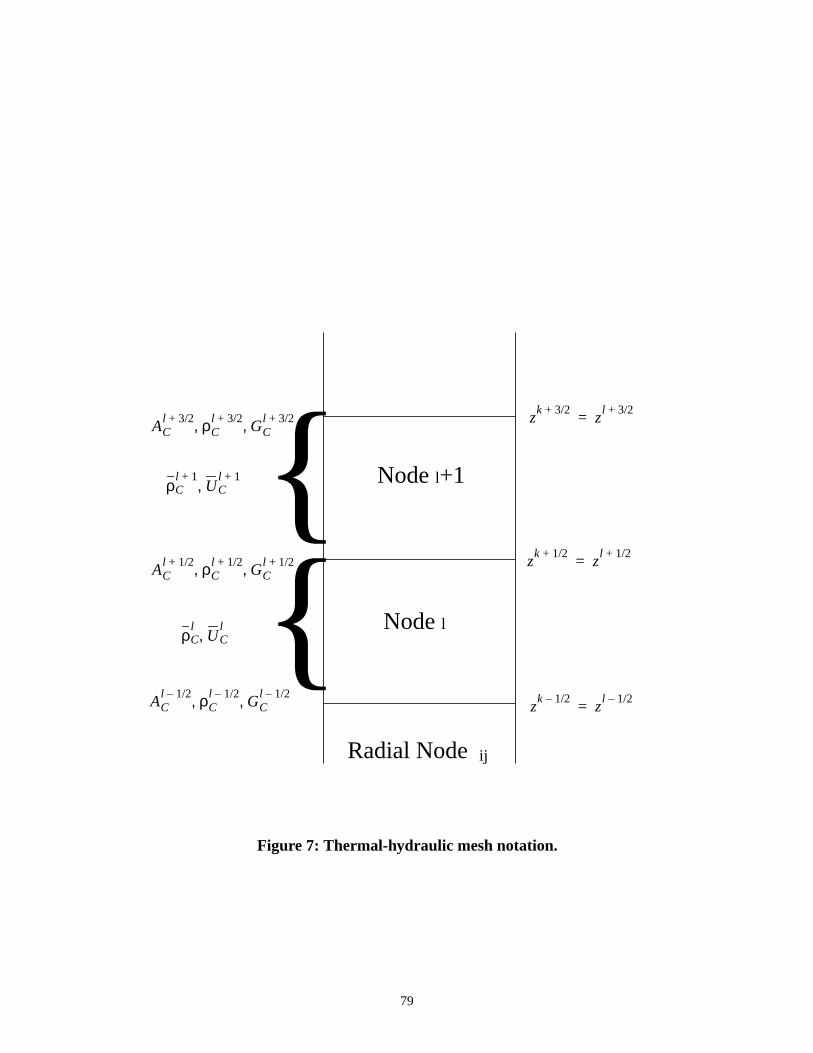
zk 3/2+
zl 3/2+
=
zk 1/2+
zl 1/2+
=
zk 1/2–
zl 1/2–
=
Nodel+1
Nodel
ACl 3/2+ ρC
l 3/2+GC
l 3/2+, ,
ρCl 1+
UCl 1+
,
ACl 1/2+ ρC
l 1/2+GC
l 1/2+, ,
ρCl
UCl
,
ACl 1/2– ρC
l 1/2–GC
l 1/2–, ,
Radial Nodeij
Figure 7: Thermal-hydraulic mesh notation.
79
r by
time
mass
sity is
is
cement
alues
to be
t node
(176)
Finally a backward difference time advancement scheme is employed producing
(177)
The energy conservation equation, Eq. (172) is discretized in a similar manne
integrating along the flow stream to eliminate the spatial derivative, and a semi-implicit
treatment is employed. The convective term is linearized by using new time-step level
velocity and past time-step level for the other parameters. Furthermore, the coolant den
assumed to be constant over the time-step interval. The result of this discretization scheme
(178)
where the time averaged terms appear as a result of the central difference time advan
treatment and are defined as
(179)
and
(180)
Note the convective and work terms in the energy equation contains fluid property v
at the node boundaries. However, as stated previously, the fluid property values are
calculated as node averages. An intuitive approach would be to spatially average adjacen
z∂∂
GCij
z t,( )ACij
z( )( )dz
zk 1/2–
zk 1/2+
∫ GCl 1/2+
t( )ACl 1/2+
GCl 1/2–
t( )ACl 1/2–
–=
VCl ρ
l n 1+,ρ
l n,–
tn∆------------------------------- GC
l 1/2,n 1+ +AC
l 1/2+GC
l 1/2,n– 1+AC
l 1/2––+ 0=
VCl ρC
l n, Ul n 1+,
Ul n,
–tn∆
---------------------------------- GCl 1 2 n 1+,⁄+
ACl 1 2⁄+
UCl 1 2 n,⁄+
GCl 1 2 n 1+,⁄–
ACl 1 2⁄–
– UCl 1 2 n,⁄+( )–=
PGC
l 1 2 n,⁄+AC
l 1 2⁄+
ρCl 1 2 n,⁄+
----------------------------------------GC
l 1 2 n,⁄–AC
l 1 2⁄–
ρCl 1 2 n,⁄–
----------------------------------------–
qSl n 1+,
SFl
zl∆ qC
l n 1+,VF
l+ +–
qSl n 1+, qS
l n,qS
l n 1+,+
2-------------------------------=
qCl n 1+, qC
l n,qC
l n 1+,+
2-------------------------------=
80

ver, it
]. The
nsity
s of
ms of
lant
bove
average property values along the flow direction to obtain the node boundary values. Howe
has been found that a donor cell averaging technique is necessary for numerical stability [17
donor cell average is defined for the coolant internal energy as
(181)
and for the coolant density as
(182)
for flow in the positive direction, the only modelling capability within NESTLE.
To solve the two coupled discretized equations, the Equation of State for coolant de
in terms of coolant internal energy is linearized as follows
(183)
This equation is then substituted into Eq. (177) to solve for the coolant mass velocity in term
coolant internal energy to produce
(184)
Finally, the above equation is substituted into Eq.(139) to produce an equation only in ter
coolant internal energy
(185)
This equation is solved for at each radial node by sweeping in the direction of coo
flow. The following auxiliary relationships are used to evaluate terms appearing in the a
UCl 1 2 n,⁄+
UCl n,
= and UCl 1 2 n,⁄–
UCl 1– n,
=
ρCl 1 2 n,⁄+ ρC
l n,= and ρC
l 1 2 n,⁄– ρCl 1– n,
=
ρCl n 1+,
ρCl n,
UCl
∂
∂ ρCl
tn
UCl n 1+,
UCl n,
–( )+≅
GCl 1 2 n 1+,⁄+ 1
ACl 1 2⁄+
----------------- GCl 1 2 n 1+,⁄–
ACl 1 2⁄– VC
l
tn∆-------
–UC
l∂
∂ ρCl
tn
UCl n 1+,
UCl n,
–( )=
VCl
tn∆-------
ρCl n, ∂ρC
l
∂UCl
-----------
tn
ACl 1 2⁄+
UCl n,
–
UCl n 1+,
GCl 1 2 n 1+,⁄–
ACl 1 2⁄–
UCl 1 n,–
UCl n,
–( )=
PGC
l 1 2 n,⁄+AC
l 1 2⁄+
ρCl n,----------------------------------------
GCl 1 2 n,⁄–
ACl 1 2⁄–
ρCl 1 n,–
----------------------------------------–
qSl n 1+,
SFl
z∆ lqC
l n 1+,VC
l VCl
tn∆-------
ρCl n,
UCl n,
+ + +–
UCl n 1+,
81

olant
olant
void
aving
equation:
Coolant Volume:
Total Fuel Rod Surface Area Per Unit Axial Length:
Coolant Volumetric Heat Source:
where
= wet fraction for the node when rodded
= fuel rod radius
= number of fuel pins within the node
= distribution fraction of energy directly deposited within the fuel
= total volumetric power density for heat deposited within the node.
Having obtained values for the coolant internal energy at the new time-step, the co
densities are evaluated at the new time-step using an Equation of State for the liquid if co
internal energy indicates sub-cooled conditions for the node. If bulk boiling is indicated, the
fraction is first determined as follows (suppressing superscripts)
(186)
where
= saturated coolant liquid internal energy
= saturated coolant vapor internal energy
= saturated coolant liquid density
= saturated coolant vapor density
from which the coolant density is determined as now indicated
(187)
These same equations are utilized in determining introduced back in Eq. (183). H
VCl
f Roddedl
Vl⋅=
SFl
2πrFNFuelPinsl
=
qCl n,
VCl
1 dF–( )qTl n,
Vl
=
f Roddedl
r F
NFuelPinsl
dF
qTl n,
αρCL
UC UCL–( )
ρCVUCV
UC–( ) ρCLUCL
UC–( )–---------------------------------------------------------------------------------=
UCL
UCV
ρCL
ρCV
ρC αρCV1 α–( )ρCL
+=
UCd
dρC
82

e new
terial
bility
ontrol
8] is
ally
ight
e-step
ilizing
sity as
nergy,
fluid.
icated
ed in
havior,
ed
evaluated the coolant density, Eq. (177) is used to solve for the coolant mass velocity at th
time-step.
The above approach is not unconditionally stable and must satisfy the Courant ma
limit due to the degree of semi-implicitness introduced in linearizing the equations. This sta
limit for certain transients restricts the time-step sizes to values smaller than required to c
truncation errors. The Stability-Enhancing Two-Step (SETS) Method developed at LANL [1
used to allow a Courant material limit violating treatment. Since this method was origin
utilized within the context of the six-equation model used within the TRAC code, a sl
modification of the SETS method is required for the current application.
The stabilizing energy conservation equation used to solve for is given by
(188)
Do note the increased degree of implicitness of this equation. Estimates of the current tim
values are determined solving the previous introduced set of equations. Having stab
predicted values of coolant internal energy, they are then utilized to update the coolant den
noted before. Also, the coolant temperature is determined based upon coolant internal e
using an Equation of State for sub-cooled fluid and the saturation temperature for saturated
This approach has been shown to allow large time-steps without stability problems, as ind
by solving the transient equations at steady-state conditions and observing no drift.
To initiate the process, the volumetric power density at the new time-step is estimat
the same manner as the flux; that is, it is time extrapolated, assuming exponential time be
using power density values atn-1 andn. The past time value of the surface heat flux is employ
UCl n 1+,
VCl ρC
l n 1+,UC
l n 1+, ρCl n,
UCl n,
–tn∆
------------------------------------------------------------
G( Cl 1 2⁄+ n 1+,
ACl 1 2⁄+
UCl n 1+,
–=
G– Cl 1 2⁄– n 1+,
ACl 1 2⁄–
UCl 1 n 1+,–
) PGC
l 1 2⁄+ n 1+,AC
l 1 2⁄+
ρCl n 1+,-----------------------------------------------
GCl 1 2 n 1+,⁄–
ACl 1 2⁄–
ρCl 1 n 1+,–
-----------------------------------------------–
–
qSl n 1+,
SFl
z∆ lqC
l n 1+,VC
l+ +
83

tions,
ed to
aulic
ith the
of the
on for
olant
values.
alues.
so all
lance
ies. In
value.
based
aging
ed
de is
le of
n each
as the initial estimate for the new time step. Using these values in the thermal-hydraulic equa
they provide initial estimates of the coolant and fuel conditions at the new time-step, us
correct cross-sections and commence the flux iterations. With the explicit thermal-hydr
option selected, these values are never updated and used throughout the flux iteration. W
implicit thermal-hydraulic option selected, the SETS process is repeated as new estimates
volumetric power density and heat flux become available, associated with the iterative soluti
the flux.
For the feedback correction of cross-sections with respect to coolant density, co
temperature, and effective fuel temperature, all must be evaluated as node average
Likewise, the coolant temperature appearing in Newton’s Law requires node average v
Previously we stated that we are solving for node average values of coolant properties,
would seem in order. However, thinking about the steady-state solution of the energy ba
equation it becomes clear that coolant internal energy is really evaluated at node boundar
this sense donoring is done counter-flow from the node boundary value to the node average
Therefore the node average coolant temperature is determined using an Equation of State
upon the average of the coolant internal energy at axial elevationsk-1 andk. The node average
coolant density used to correct cross-sections follows a similar approach, now directly aver
densities. This subtlety becomes important for large axial meshing (e.g. 2D radial geometry).
II.9.c. Fuel Temperature Model
The lumped (i.e. radially averaged) fuel temperature is obtained by utilizing a lump
parameter heat conduction model, in which a simple energy balance for each radial no
performed. This approach should be valid for transients where the fuel pin-wise radial profi
the fuel temperature stays close to the steady-state profile. The rate of energy change i
84

de heat
ces
sity is
91) to
e
ge fuel
node, ignoring axial heat conduction, can be expressed as the difference between the no
source and the energy lost due to heat transported radially:
(189)
where r denotes the radial coordinate for an average pin in node ij and
= fuel internal energy
= fuel density
= volumetric power density from heat deposited directly in the fuel
= heat flux within the fuel
Using Fourier’s Law of Thermal Conductivity expresses the heat flux within the fuel as
(190)
wherekF denotes the fuel’s thermal conductivity. Substituting Eq. (190) into Eq. (189) produ
(191)
The enthalpy is now expressed in terms of the fuel specific heat ( ) and temperature, den
assumed constant, and fuel specific heat is assumed slowly varying in time allowing Eq. (1
be rewritten as
(192)
Integrating over the nodel volume occupied by fuel, denoted,
(193)
where indicates the fraction of nodel occupied by fuel, applying the central difference tim
advancement scheme, and rearranging terms yields the final expression for the node avera
temperature.
qFij
r z t, ,( )
t∂∂ ρF
ijr z t, ,( )UF
ijr z t, ,( )( ) qF
ijr z t, ,( ) ∇r qhf
ijr z t, ,( )⋅–=
UFij
ρFij
qFij
qhfij
qhfij
r z t, ,( ) k– Fij
r z t, ,( )∇rTFij
r z t, ,( )=
t∂∂ ρF
ijr z t, ,( )UF
ijr z t, ,( )( ) qF
ijr z t, ,( ) ∇r kF
ijr z t, ,( )∇rTF
ijr z t, ,( )⋅+=
cpF
ρFcPF
ijr z t, ,( )
∂TFij
r z t, ,( )∂t
---------------------------- qFij
r z t, ,( ) ∇r kFij
r z t, ,( )∇rTFij
r z t, ,( )⋅+=
VFl
f Fl
Vl×=
f Fl
85
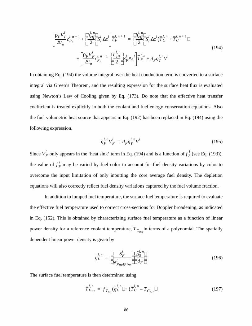
rface
luated
sfer
Also
ing the
93)),
r to
tion
ion.
luate
icated
linear
tially
(194)
In obtaining Eq. (194) the volume integral over the heat conduction term is converted to a su
integral via Green’s Theorem, and the resulting expression for the surface heat flux is eva
using Newton’s Law of Cooling given by Eq. (173). Do note that the effective heat tran
coefficient is treated explicitly in both the coolant and fuel energy conservation equations.
the fuel volumetric heat source that appears in Eq. (192) has been replaced in Eq. (194) us
following expression.
(195)
Since only appears in the ‘heat sink’ term in Eq. (194) and is a function of (see Eq. (1
the value of may be varied by fuel color to account for fuel density variations by colo
overcome the input limitation of only inputting the core average fuel density. The deple
equations will also correctly reflect fuel density variations captured by the fuel volume fract
In addition to lumped fuel temperature, the surface fuel temperature is required to eva
the effective fuel temperature used to correct cross-sections for Doppler broadening, as ind
in Eq. (152). This is obtained by characterizing surface fuel temperature as a function of
power density for a reference coolant temperature, in terms of a polynomial. The spa
dependent linear power density is given by
(196)
The surface fuel temperature is then determined using
(197)
ρFVFl
tn∆--------------cPF
l n 1+, heffl n,
2--------
SFl
zl∆+ TF
l n 1+, heffl n,
2--------
SFl
zl∆ TC
l n,TC
l n 1+,+( )=
ρFVFl
tn∆--------------cPF
l n 1+, heffl n,
2--------
– SFl
zl∆ TF
l n,dFqT
l n,V
l+ +
qFl n,
VFl
dFqTl n,
Vl
=
VFl
f Fl
f Fl
TCRef
qLl n, SF
l
NFuelPinsl
---------------------- qS
l n,
dF--------
=
TFSrf
l n,f TSrf
qLl n,
( ) TCl n,
TCRef–( )+=
86

d fuel
n the
locity
noring
mporal
ons are
of the
ansfer
ficient
where denotes the polynomial function.
II.9.d. Steady-State Model
For steady-state conditions, the governing equations used to solve for the coolant an
conditions are obtained by setting the temporal derivative to zero. When this is done i
coolant’s mass continuity equation, Eq. (171), it is seen that the product of coolant mass ve
and cross-sectional flow area must be constant up the flow channel. Also the concept of do
no longer enters since node average coolant values only appeared because of the te
derivative terms. These implications lead to the following discretized equations:
Coolant Mass Continuity
(198)
where subscript In denotes the inlet to radial node ij associated with node l.
Coolant Energy Conservation
(199)
Fuel Energy Conservation
(200)
Surface fuel temperature is evaluated as indicated for the transient conditions. These equati
iteratively solved as new estimates of the flux become available, providing new estimates
surface heat flux and volumetric heat densities. During these iterations the effective heat tr
coefficient is also updated, producing consistent values for the effective heat transfer coef
f TSrfqL
l n,( )
GCl 1 2⁄+ AC
l 1 2⁄–
ACl 1 2⁄+
-----------------
GCl 1 2⁄– ACIn
ij
ACl 1 2⁄+
-----------------
GCIn
ij= =
UCl 1 2⁄+
UCl 1 2⁄–
PACIn
ijGCIn
ij 1
ρCl 1 2⁄+
----------------- 1
ρCl 1 2⁄–
----------------–
qCl
VCl
qFlVF
l+ +–=
TFl
TCl VF
l
heffl
SFl
zl∆
-----------------------
qFl
+=
87

cient
fficient
rmined
ws.
and
d by
itial
. Now
e node
olution
raulic
n, but
heat
e fuel
and lumped fuel temperature as now described.
II.9.e. Effective Heat Transfer Coefficient Evaluation
For the lumped fuel temperature model to be utilized, the effective heat transfer coeffi
must be evaluated. For steady-state conditions we can select the effective heat transfer coe
such that the correct values of the lumped fuel temperature result, these temperatures dete
utilizing a more detailed fuel pellet model. This implies the following:
(201)
One can now solve forheff given values of and for a fixed coolant temperature as follo
(202)
Note thatheff has been characterized as a function of since the fuel thermal conductivity
gap closure, both functions of fuel temperature, are the main reasons whyheff changes. This
characterization is captured using a polynomial representation.
For steady-state calculations, an initial estimate of fuel temperature is obtaine
characterizing it as a function of linear power density in terms of a polynomial. Given this in
lumped fuel temperature estimate, the effective heat transfer coefficient can be evaluated
Eq. (200) can be used to calculate a new estimate of the lumped fuel temperature once th
average coolant temperature and volumetric heat density have been evaluated. As the flux s
is iterated, this sequence of calculations is repeated. The iteration of the thermal-hyd
equations not only addresses feedback between its solution and the neutronic solutio
addresses the non-linearities in calculating the lumped fuel temperature due to effective
transfer coefficient dependency on fuel temperature.
For transient calculations, the same iterative sequence is employed; however, now th
qF AF heffSF TF TCRef–( )=
TF qF
heff
qF AF
SF TF TCRef–( )
------------------------------------=
TF
88
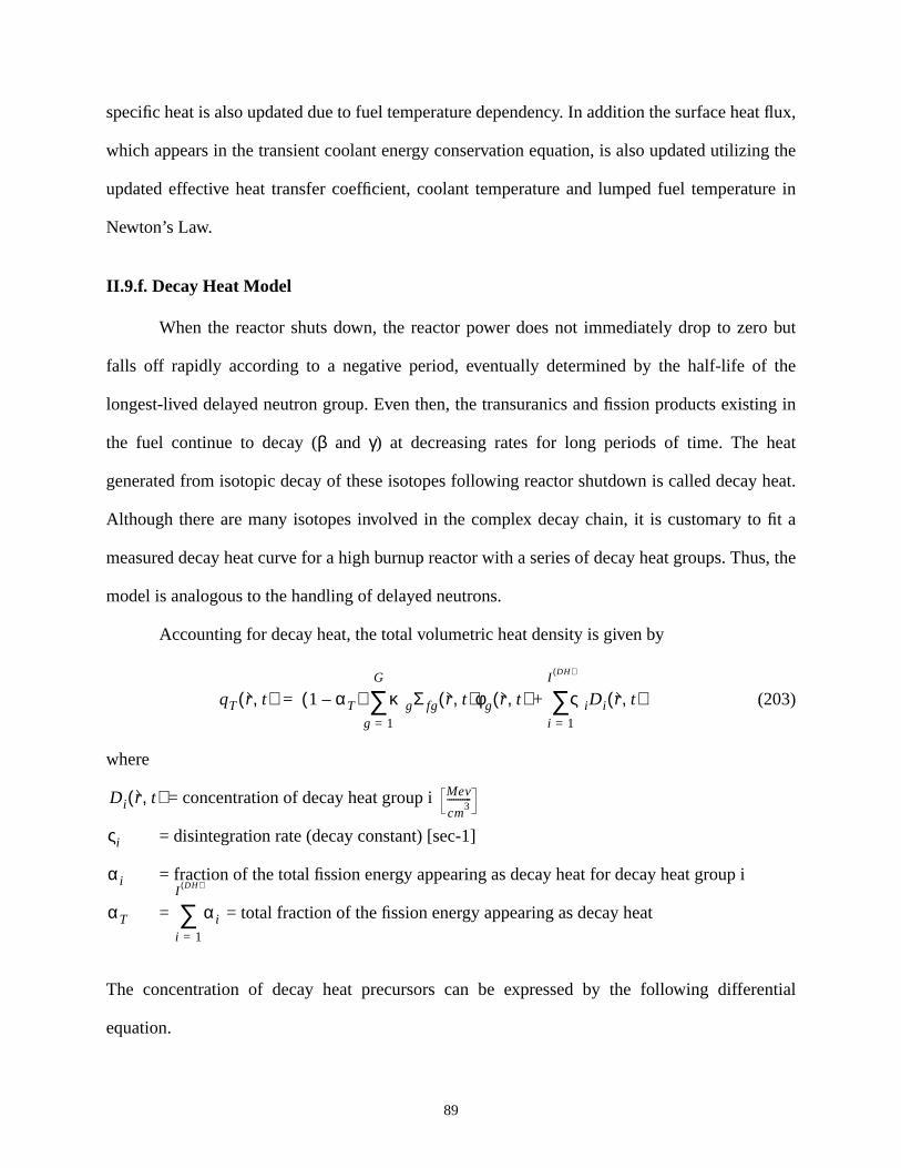
at flux,
ng the
ture in
o but
the
ting in
at
heat.
fit a
us, the
ential
specific heat is also updated due to fuel temperature dependency. In addition the surface he
which appears in the transient coolant energy conservation equation, is also updated utilizi
updated effective heat transfer coefficient, coolant temperature and lumped fuel tempera
Newton’s Law.
II.9.f. Decay Heat Model
When the reactor shuts down, the reactor power does not immediately drop to zer
falls off rapidly according to a negative period, eventually determined by the half-life of
longest-lived delayed neutron group. Even then, the transuranics and fission products exis
the fuel continue to decay (β and γ) at decreasing rates for long periods of time. The he
generated from isotopic decay of these isotopes following reactor shutdown is called decay
Although there are many isotopes involved in the complex decay chain, it is customary to
measured decay heat curve for a high burnup reactor with a series of decay heat groups. Th
model is analogous to the handling of delayed neutrons.
Accounting for decay heat, the total volumetric heat density is given by
(203)
where
= concentration of decay heat group i
= disintegration rate (decay constant) [sec-1]
= fraction of the total fission energy appearing as decay heat for decay heat group i
= = total fraction of the fission energy appearing as decay heat
The concentration of decay heat precursors can be expressed by the following differ
equation.
qT r t,( ) 1 αT–( ) κgΣ fg r t,( )g 1=
G
∑ φg r t,( ) ςiDi r t,( )i 1=
I DH( )
∑+=
Di r t,( ) Mev
cm3
-----------
ςi
αi
αT αii 1=
I DH( )
∑
89

grated
ource
nterval
sired
rium.
4) and
.
(204)
To develop an expression for the decay heat precursor concentrations, a time-inte
expression is derived by integrating Eq. (204) from tn to tn+1. This integration results in
(suppressing dependence for clarity)
(205)
To solve the above integral, a functional form for the time dependent neutron fission s
density must be developed. Assume the fission source density is constant over the time i
at the past time-step value,i.e.
(206)
Incorporating this approximation into Eq. (205) and rearranging terms we obtain the de
expression.
(207)
In steady-state it is generally assumed that even the longest-lived group is in equilib
The steady-state concentration is calculated by setting the time derivative to zero in Eq. (20
solving for the precursor concentration producing,
(208)
This equation is utilized to determine the initial conditions required for the transient solution
∂Di r t,( )∂t
--------------------- αi κgΣ fg r t,( )φg r t,( ) ςiDi r t,( )–g 1=
G
∑= for i 1,...,IDH( )
=
r
Di tn 1+( ) Di tn( )eςi tn∆–
αi κgΣ fg t′( )φg t′( )eςi– tn 1+ t′–( )
dt′g 1=
G
∑tn
tn 1+
∫+=
t′ tn tn 1+,[ ]∈
κgΣ fg t′( )φg t′( )g 1=
G
∑ κgΣ fg tn( )φg tn( )g 1=
G
∑=
Di tn 1+( ) Di tn( )eςi tn∆– αi
ςi----- 1 e
ςi tn∆––[ ] κgΣ fg tn( )φg tn( )
g 1=
G
∑+=
Di∞
αi
ςi----- κgΣ fgφg
g 1=
G
∑=
90
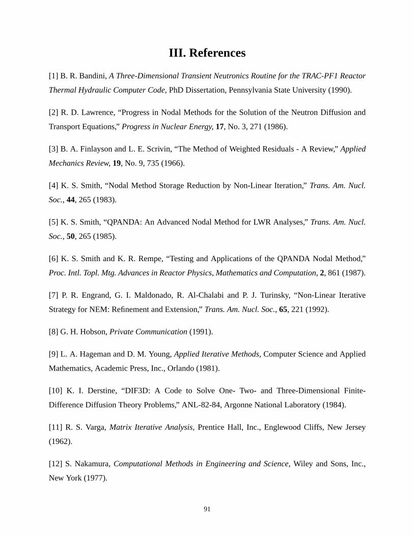
ctor
and
d,”
tive
te-
y
III. References
[1] B. R. Bandini,A Three-Dimensional Transient Neutronics Routine for the TRAC-PF1 Rea
Thermal Hydraulic Computer Code, PhD Dissertation, Pennsylvania State University (1990).
[2] R. D. Lawrence, “Progress in Nodal Methods for the Solution of the Neutron Diffusion
Transport Equations,”Progress in Nuclear Energy, 17, No. 3, 271 (1986).
[3] B. A. Finlayson and L. E. Scrivin, “The Method of Weighted Residuals - A Review,”Applied
Mechanics Review, 19, No. 9, 735 (1966).
[4] K. S. Smith, “Nodal Method Storage Reduction by Non-Linear Iteration,”Trans. Am. Nucl.
Soc., 44, 265 (1983).
[5] K. S. Smith, “QPANDA: An Advanced Nodal Method for LWR Analyses,”Trans. Am. Nucl.
Soc., 50, 265 (1985).
[6] K. S. Smith and K. R. Rempe, “Testing and Applications of the QPANDA Nodal Metho
Proc. Intl. Topl. Mtg. Advances in Reactor Physics, Mathematics and Computation, 2, 861 (1987).
[7] P. R. Engrand, G. I. Maldonado, R. Al-Chalabi and P. J. Turinsky, “Non-Linear Itera
Strategy for NEM: Refinement and Extension,”Trans. Am. Nucl. Soc., 65, 221 (1992).
[8] G. H. Hobson,Private Communication(1991).
[9] L. A. Hageman and D. M. Young,Applied Iterative Methods, Computer Science and Applied
Mathematics, Academic Press, Inc., Orlando (1981).
[10] K. I. Derstine, “DIF3D: A Code to Solve One- Two- and Three-Dimensional Fini
Difference Diffusion Theory Problems,” ANL-82-84, Argonne National Laboratory (1984).
[11] R. S. Varga,Matrix Iterative Analysis, Prentice Hall, Inc., Englewood Cliffs, New Jerse
(1962).
[12] S. Nakamura,Computational Methods in Engineering and Science, Wiley and Sons, Inc.,
New York (1977).
91

ith
-5,”
nal
al
- I:
-II:
al-
M-
of
,”
[13] S. K. Zee,Numerical Algorithms for Parallel Processors Computer Architectures w
Applications to the Few-Group Neutron Diffusion Equations, PhD thesis, North Carolina State
University (1987).
[14] L. A. Hageman and C. J. Pfeifer, “The Utilization of the Neutron Diffusion Program PDQ
WAPD-TM-385, Bettis Atomic Power Laboratory, Westinghouse Power Corporation (1965).
[15] R. D. Lawrence, “The DIF3D Nodal Neutronics Option for Two- and Three-Dimensio
Diffusion-Theory Calculations in Hexagonal Geometry,” ANL-83-1, Argonne Nation
Laboratory (1983).
[16] Y. Chao and N. Tsoulfanidis, “Conformal Mapping and Hexagonal Nodal Methods
Mathematical Foundation,”Nucl. Sci. Eng., 121, 202-209 (1995).
[17] Y. Chao and Y.A. Shattila, “Conformal Mapping and Hexagonal Nodal Methods
Implementation in the ANC-H Code,” Nucl. Sci. Eng., 121, 210-225 (1995).
[18] M. Knight , P. Hutt, and I. Lewis, “Comparison of PANTHER Nodal Solutions in Hexagon
z Geometry,”Nucl. Sci. Eng., 121, 254-263 (1995).
[19] R. F. Barry, “LEOPARD - A Spectrum Dependent Non-Spatial Depletion Code for the IB
7094,” WCAP-3269-26, Atomic Power Division, Westinghouse Electric Corporation (1963).
[20] T. A. Porsching, J. H. Murphy and J. A. Redfield, “Stable Numerical Integration
Conservation Equations for Hydraulic Networks,”Nuclear Science and Engineering, 43, 218
(1971).
[21] J. H. Mahaffy, “A Stability-Enhancing Two-Step Method for Fluid Flow Calculations
Journal of Computational Physics, 46, 239 (1982).
92
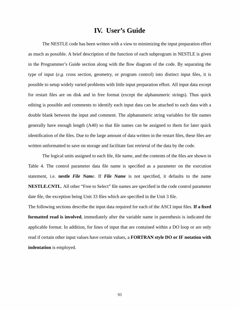
ffort
given
g the
is
cept
quick
with a
ames
quick
s are
wn in
cution
e
eter
the
nly
IV. User’s Guide
The NESTLE code has been written with a view to minimizing the input preparation e
as much as possible. A brief description of the function of each subprogram in NESTLE is
in the Programmer’s Guide section along with the flow diagram of the code. By separatin
type of input (e.g. cross section, geometry, or program control) into distinct input files, it
possible to setup widely varied problems with little input preparation effort. All input data ex
for restart files are on disk and in free format (except the alphanumeric strings). Thus
editing is possible and comments to identify each input data can be attached to each data
double blank between the input and comment. The alphanumeric string variables for file n
generally have enough length (A40) so that file names can be assigned to them for later
identification of the files. Due to the large amount of data written in the restart files, these file
written unformatted to save on storage and facilitate fast retrieval of the data by the code.
The logical units assigned to each file, file name, and the contents of the files are sho
Table 4. The control parameter data file name is specified as a parameter on the exe
statement, i.e.nestle File Name. If File Name is not specified, it defaults to the nam
NESTLE.CNTL . All other “Free to Select” file names are specified in the code control param
date file, the exception being Unit 33 files which are specified in the Unit 3 file.
The following sections describe the input data required for each of the ASCI input files.If a fixed
formatted read is involved, immediately after the variable name in parenthesis is indicated
applicable format. In addition, for lines of input that are contained within a DO loop or are o
read if certain other input values have certain values, aFORTRAN style DO or IF notation with
indentation is employed.
93
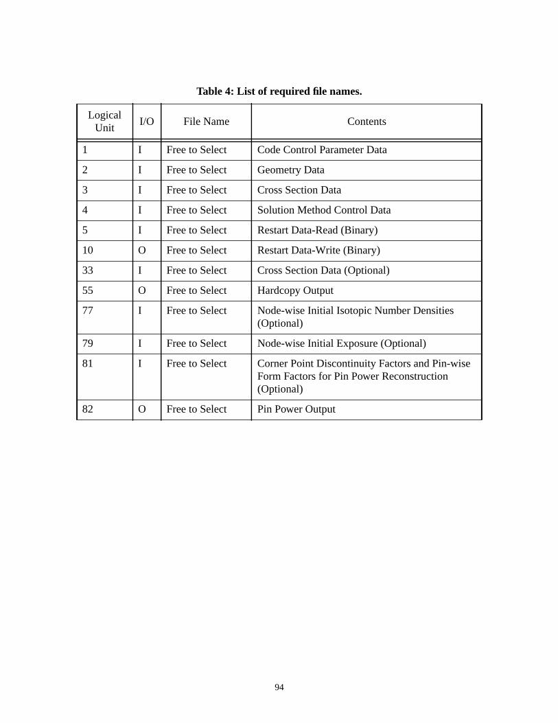
Table 4: List of required file names.
LogicalUnit
I/O File Name Contents
1 I Free to Select Code Control Parameter Data
2 I Free to Select Geometry Data
3 I Free to Select Cross Section Data
4 I Free to Select Solution Method Control Data
5 I Free to Select Restart Data-Read (Binary)
10 O Free to Select Restart Data-Write (Binary)
33 I Free to Select Cross Section Data (Optional)
55 O Free to Select Hardcopy Output
77 I Free to Select Node-wise Initial Isotopic Number Densities(Optional)
79 I Free to Select Node-wise Initial Exposure (Optional)
81 I Free to Select Corner Point Discontinuity Factors and Pin-wiseForm Factors for Pin Power Reconstruction(Optional)
82 O Free to Select Pin Power Output
94
ation
IV.1. Code Control Parameter Data File
(Unit 1 => “CNTRL”)
TITLE (A80)
Title line to identify run in hardcopy output
NBUSTEP
Maximum of the number of burnup mask values input for the soluble poison concentr
or (burnup steps+1).
NBMAX
Maximum number of control rod banks (groups) to be input.
GEOM (A40)
Geometry data file name (Unit 2)
XSECT (A40)
Cross section data file name (Unit 3)
KINET (A40)
Kinetic data file name (Unit 4)
PERFM (A40)
Solution method control file name (Unit 5)
RESTRT (A40)
Restart file name [to read] (Unit 9)
OUTPUT (A40)
Hardcopy output file name (Unit 55)
OUTADJ (A40)
Unformatted output file name for adjoint solution (Unit 10)
IADJ (A5)
Adjoint option (“Y”/ “N”)
95

ISAVEADJ (A5)
Write adjoint solution to file OUTADJ (“Y”/ “N”)
ITRAN (A5)
Transient option (“Y”/ “N”)
IRSTRT (A5)
Restart option (“Y”/ “N”)
ITYPE (A5)
Problem type
Eigenvalue (“EVP”)
Fixed-source (“FSP”)
NXSEC (A5)
Cross-section corrections to be applied (“Y”/ “N”)
IF (NXSEC.EQ. “Y”) THEN READ
ASRCH (A5)
Criticality/Power level search option (“Y”/ “N”)
IF (ASRCH.EQ. “Y”) THEN READ
IWHICH
Parameter to search upon
Power level (relative)=1
Soluble poison concentration (PPM)=2
Coolant inlet temperature (oF)=3
Lead (I.D.=highest value) control bank withdrawn (inches)=4
IF(ITYPE.EQ.”EVP’) THEN READ
CKE_TARGET
Target keff value to match in search
96

ENDIF EVP
ENDIF ASRCH
ANFDBK (A5)
Thermal-hydraulic feedback on (“Y”/ “N”)
ENDIF NXSEC
ABUCKL (A5)
Buckling correction option to be applied (“Y”/ “N”)
AVEBU(1)
Cycle average burnup at first burnup step (MWD/MTM)
IBURN (A5)
Depletion case (“Y”/ “N”)
IF (IBURN.EQ. “Y”) THEN READ
NBU
Number of burnup steps
(DELBU(I),I=2,NBU+1)
Burnup steps’ sizes (MWD/MTM)
ENDIF IBURN
(IXE(I), I=1,NBU)
Xenon-samarium conditions for each burnup step
No Xe and Sm = 1
Freeze Xe and Sm = 2
Equilibrium Xe and Sm = 3
No Xe and transient Sm = 4
Transient Xe and Sm = 5
No Xe and freeze Sm = 6
97

t
,
BP,
IF (NXSEC.EQ. “Y”) THEN READ
NPPMX
Number of burnup steps that letdown soluble poison concentration provided a
DO IBU=1,NPPMX
BUPM(IPM),PPM(IPM)
Cycle burnup (MWD/MTM) and soluble poison concentration (PPM)
ENDDO IBU ...Burnup step loop
(ZB(IBK),IBK=1,NBMAX)
Control banks (group) axial withdrawal position (in)
PRCNT
Power level (% of full rated)
ENDIF NXSEC
AL3 (A5)
Long input echo options: Yes/No (“Y”/ “N”)
NPC (A5)
Long hardcopy output option (“Y”/ “N”)
IF (NPC.EQ. “Y”)THEN READ
NOUTLONG
Number of variables whose node values are to be output
(AOUTLONG(N),N=1,NOUTLONG) (10(A5,1X))
Names of variables whose node values are to be output
PREL, FLUX, DCOOL, TCOOL, TFUEL, BU, I135, XE135, PM149, SM149
U234, U235, U236, U238, PU239, PU240, PU241, PU242, LFPG1, LFPG2,
ADJFL
ENDIF NPC
98

by
ut
save
CRTON (A5)
CRT output option (“Y”/ “N”)
DO IBU=1,NBU+1...For each burnup step
ISAVE(IBU) (A5)
Write steady-state restart file (“Y”/”N”) at burnup step IBU
IF (ISAVE(IBU).EQ. “Y”) THEN READ
OUT(IBU) (A40)
Steady-state restart file name [to write] at burnup step IBU
ENDIF ISAVE(IBU)
ENDDO IBU ...Burnup step loop
IF (ITRAN.EQ. “Y”) THEN READ
ISAVETR (A5)
Write transient restart file (“Y”/”N”)
ENDIF ITRAN
IF (ISAVETR.EQ. “Y”) THEN READ
OUTTR (A40)
Transient restart file name [to write]. This file is written at every time indicated
the kinetic file input variable TIMEPR(IT), that indicates times when outp
should be produced. Note transient restart file is overwritten each time to
space.
ENDIF ISAVETR
IEXP (A5)
Initial node-wise exposure map available (“Y”/ “N”)
IF (IEXP.EQ. “Y”) THEN READ
FINITEXP (A40)
99

-at the
nal
)
rm
Name of the file containing the initial node-wise exposures (Unit=79)
ENDIF IEXP
OEOC (A5)
End of depletion ASCII restart file option (“Y” / “N”)
If OEOC = “Y”, NESTLE will write new code control parameter file (CNTRL file), nodewise exposure map, and node-wise number density map (for microscopic depletion)end of the depletion. This option is valid for a steady-state problem only.
Note: the following pin power reconstruction option is currently available for hexago
geometry only.
PPR (A5)
Pin power reconstruction option (“Y”/ “N”)
IF (PPR.EQ. “Y”) THEN READ
FPIN (A5)
Corner point discontinuity factors and pin-wise form factors available (“Y”/ “N”
IF (FPIN.EQ. “Y”) THEN READ
INPPIN (A40)
File name containing the corner point discontinuity factors and pin-wise fo
factors (Unit=81)
ELSEIF (FPIN.EQ. “N”) THEN READ
NHRPIN
Number of radial rings of pins surrounding center pin.
Number of pins within the assembly = NPIN
When PPR = “Y” and FPIN = “N”, NESTLE will set all corner point
NPIN 6 ii 1=
NHRPIN 1–
∑ 1+=
100

discontinuity factors and form factor values to 1.0.
ENDIF FPIN
OUTPPR (A5)
Output pin-wise power values (“Y” / “N”)
IF (OUTPPR.EQ. “Y”) THEN READ
OUTPIN (A40)
Pin power output file name (Unit=82)
ENDIF OUTPPR
ENDIF PPR
101

ions.
IV.2. Geometry Data File
(Unit 2 => “GEOM”)
NSHAP (A5)
Node shape in radial plane
Hexagonal (“HEXA”)
Cartesian (“CART”)
IDRUN (A5)
Core symmetry
IF (NSHAP .EQ. “HEXA”)
Full core (“FCORE”)
One-third core (“TCORE”) 5 to 9 o’clock
One-sixth core (“SCORE”) 5 to 7 o’clock
One-dimensional axial core (“AXIAL”)
IF (NSHAP. EQ. “CART”)
Full core (“FCORE”)
Half core (“HCORE”) 3 to 9 o’clock
Quarter core (“QCORE”) 3 to 6 o’clock
One-dimensional axial core (“AXIAL”)
ENDIF NSHAP
IF (NSHAP.EQ."CART") THEN READ
NX,NY
The x and y total mesh numbers applicable to initial homogenous material reg
NMULXY
Number of mesh to create from each input x and y material mesh.
ELSEIF (NSHAP.EQ."HEXA") THEN READ
102

all
n.
al
e
NHR
Number of radial rings of bundles (assemblies) surrounding center bundle.
ENDIF NSHAP
NZ
The z total mesh number applicable to initial material regions.
NMULZ
Number of mesh to create from each input z material mesh.
NFIGURE
Number of different radial configurations (basic figures) of core materials over
elevation.
LIHO,LIPS,LIZU,LIZD
Boundary conditions: Radial exterior, radial interior, z-up, z-down
(reflective=0, zero flux=1, non-reentrant=2, cyclic=3, not applicable=4)
For radial exterior, z-up and z-down boundaries, LIHO cannotequal 3.
IF(NSHAP.EQ."CART") THEN READ
BPITCHX,BPITCHY
Pitch for bundles (assemblies) in the x and y directions (in).
NSUBX,NSUBY
Number of different x and y material mesh sizes to utilize in numerical solutio
(NSPACX(I),DDX(I),I=1,NSUBX)
Number of consecutive x material mesh (NSPACX(I)) of constant x mesh size
(DDX(I)) running from west to east. [Note the sum of NSPACX(I) must equ
NX.]
(NSPACY(J),DDY(J),J=1,NSUBY)
Number of consecutive y material mesh (NSPACY(J)) of constant y mesh siz
103

ual
al
(DDY(J)) running from north to south. [Note the sum of NSPACY(J) must eq
NY.]
ELSEIF (NSHAP.EQ."HEXA") THEN READ
DELH
Pitch of bundles (assemblies) (in)
ENDIF NSHAP
(See section IV.2.a entitled Geometry Input for detailed description of geometry input.)
DO IB=1,NFIGURE ...For each color figure
NBASIC(IB)
Basic figure I.D. (=1,2,...)
DO IY=1,NY...For each y mesh
(NCOL2DT(IX,IY,IB), IX=NXSTART(IY),NXEND(IY),NXSKIP)
Core material colors defined for initial radial material mesh.
ENDDO...Y mesh loop
ENNDO...Color figure loop
Blank Line
DO IY=1,NY...For each y mesh
(NROT2DT(IX,IY),IX=NXSTART(IY),NXEND(IY),NXSKIP)
Mesh clockwise rotation of core material used to define surface ADFs for initi
radial material mesh.
(Cartesian: 0o = 0, 90o = 1, 180o = 2, 270o = 3)
(Hexagonal: 0o = 0, 60o = 1, 120o = 2, 180o = 3, 240o = 4, 300o = 5)
ENDDO IY
Blank Line
DO IY=1,NY
104

(K))
(NREF2DT(IX,IY),IX=NXSTART(IY),NXEND(IY),NXSKIP)
Mesh diagonal axis reflection of core material used to define surface ADFs
for initial radial material mesh. (No reflection = 0,
Reflection about NW to SE node diagonal of original orientation = 1)
ENDDO IY
NSUBZ
Number of different z material mesh sizes to utilize in numerical solution.
(NSPACZ(K),DDZ(K),K=1,NSUBZ)
Number of consecutive z material mesh (NSPACZ(K)) of constant z mesh size (DDZ
running from down to up. [Note the sum of NSPACZ(K) must equal NZ.]
IZCOLS,IZCOLE
Starting and ending axial material mesh numbers for fuel.
(NCOLZT(IZ),IZ=1,NZ)
Basic figure I.D. assigned to initial axial material mesh.
Blank Line
(NTOPZT(IZ),IZ=1,NZ)
Mesh axial reflection of core material used to define surface ADFs for initial
axial material mesh. (Up and down surfaces’ ADFs reversed)
IF (NXSEC.EQ."Y") THEN READ
Blank Line
DO IY=1,NY...For each y mesh
(LROD2DT(IX,IY),IX=NXSTART(IY),NXEND(IY),NXSKIP)
Control bank (group) I.D. defined for radial material mesh.
(Bank Present=1, 2,...,NBACU, Bank Not Present=0)
ENDDO...Y mesh loop
105

RODOFFSET
Elevation above bottom of fuel when control bank fully inserted (in).
ENDDO NXSEC
DO IY=1,NY...For each y mesh
(LSEXT2DT(IX,IY),IX=NXSTART(IY),NXEND(IY),NXSKIP)
External source locations defined for radial material mesh
(Source Present=1, Source Not Present=0)
ENDDO IY
Blank Line
(LSEXTZT(IZ),IZ=1,NZ)
External source locations defined for axial material mesh.
(Source Present=1, Source Not Present=0)
106

et
ape
ian-Z
ne-
full
axial
etries.
ed on
the
ted for
mesh
X,NY)
. For
undle
nds to
This
ndary
core
in the
ctions
IV.2.a. Geometry Input
To simplify the input of geometric information, NESTLE utilizes a highly flexible and y
automated input approach. The required input is all provided on Unit 2 => “GEOM”. Core sh
(NSHAP) can be either Cartesian-Z or Hexagonal-Z. Core symmetries (IDRUN) for Cartes
include the following: full core, half core (3 to 9 o’clock), quarter core (3 to 6 o’clock), and o
dimensional axial core. Core symmetries (IDRUN) for Hexagonal-Z include the following:
core, one-third core (5 to 9 o’clock), one-sixth core (5 to 7 o’clock), and one-dimensional
core. Figure (8) shows examples of radial material geometry figures for each of these geom
If the number of axial mesh points is set to one and reflective boundary conditions are utiliz
z-up and z-down surfaces, a two-dimensional model results.
The number of homogenous material region mesh points input in conjunction with
above core shape and symmetry input is used to automatically determine the input expec
the geometry figures. For Cartesian-Z core shape the number of x (NX) and y (NY) material
dictates the Cartesian core layout and hence geometry figures. Figure (8) corresponds to (N
= (36,36), (36,18) and (18,18) for the full, half and quarter core problems, respectively
Hexagonal-Z core shape the number of radial rings of bundles surrounding the central b
(NHR) dictates the hexagonal core layout and hence geometry figures. Figure (8) correspo
NHR = 10. Note in both these figures the ‘0’ entries in certain material mesh locations.
indicates to the NESTLE code the edge of the geometry to be analyzed where bou
conditions will be applied.It is required that every material mesh that is created from the
core shape, symmetry and material mesh number input have a value input for all geometry
figure inputs.
The material mesh sizes are determined based upon input. For the Hexagonal-Z
shape, the bundle pitch (DELH) uniquely specifies radial mesh size. Variable mesh sizes
axial direction are allowed. For the Cartesian-Z core shape, variable mesh sizes in all dire
107

each
Y and
BX,
irection
k and
input
iables
d z-
core
r core
xterior
entrant
ly be
ial
are
gure
ndle
ed to
pe and
the
(i.e.x, y and z) are allowed. Rather than requiring mesh sizes in each direction to be input for
mesh, mesh sizes are input separately for each direction with the span (NSPACX, NSPAC
NSPACZ) and size (DDX, DDY and DDZ) of a fixed mesh size input over all spans (NSU
NSUBY and NSUBZ).
To facilitate mesh refinementfor Cartesian-Z core shape only, from every initial
homogenous material mesh, refined numerical solution meshes can be generated in each d
(i.e. x, y and z) each with the same properties as the original material mesh. Feedbac
depletion effects will than be applied to the refined numerical solution mesh. This simplifies
and is very convenient when running fine-mesh benchmarks using the FDM. The input var
NMULXY and NMULZ provide the required information to complete the mesh refinement.
Boundary conditions are specified in terms of radial exterior, radial interior, z-up an
down boundaries. The radial exterior and interior boundaries locations depend upon the
shape and symmetry specified. For example, with Cartesian-Z core shape and quarte
symmetry the interior boundaries correspond to the north and west surfaces and the e
boundaries correspond to the south and east surfaces. Reflective, zero current, non-re
current and cyclic boundary conditions are treated. The cyclic boundary condition may on
used on the radial interior boundaries.
Cross-section (e.g. fuel) colors are input via geometry figures for each unique rad
configuration (NCOL2DT) as shown in Figure (8). These radial material geometry figures
than assigned to the axial material mesh via an axial mask (NCOLZT). A similar geometry fi
input style is used for all input quantities that are spatially dependent.
The final point to note with regard to geometry input concerns NESTLE’s usage of bu
pitch (i.e.BPITCHX and BPITCHY) for Cartesian-Z core shape. These variables are only us
determine the fuel bundle boundaries used in the control of output edits. Given the core sha
symmetry, mesh size and layout, and bundle pitch, NESTLE will automatically determine
108
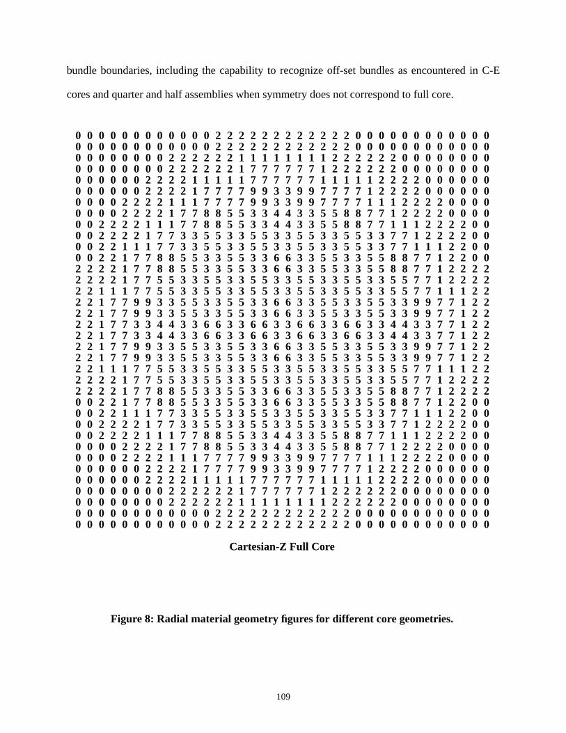
n C-E
0 0 0 0 0 0 0 0 0 0 0 0 2 2 2 2 2 2 2 2 2 2 2 2 0 0 0 0 0 0 0 0 0 0 0 0
bundle boundaries, including the capability to recognize off-set bundles as encountered i
cores and quarter and half assemblies when symmetry does not correspond to full core.
0 0 0 0 0 0 0 0 0 0 0 0 2 2 2 2 2 2 2 2 2 2 2 2 0 0 0 0 0 0 0 0 0 0 0 0 0 0 0 0 0 0 0 0 0 0 0 2 2 2 2 2 2 2 2 2 2 2 2 0 0 0 0 0 0 0 0 0 0 0 0 0 0 0 0 0 0 0 2 2 2 2 2 2 1 1 1 1 1 1 1 1 2 2 2 2 2 2 0 0 0 0 0 0 0 0 0 0 0 0 0 0 0 2 2 2 2 2 2 1 7 7 7 7 7 7 1 2 2 2 2 2 2 0 0 0 0 0 0 0 0 0 0 0 0 0 2 2 2 2 1 1 1 1 1 7 7 7 7 7 7 1 1 1 1 1 2 2 2 2 0 0 0 0 0 0 0 0 0 0 0 2 2 2 2 1 7 7 7 7 9 9 3 3 9 9 7 7 7 7 1 2 2 2 2 0 0 0 0 0 0 0 0 0 2 2 2 2 1 1 1 7 7 7 7 9 9 3 3 9 9 7 7 7 7 1 1 1 2 2 2 2 0 0 0 0 0 0 0 2 2 2 2 1 7 7 8 8 5 5 3 3 4 4 3 3 5 5 8 8 7 7 1 2 2 2 2 0 0 0 0 0 2 2 2 2 1 1 1 7 7 8 8 5 5 3 3 4 4 3 3 5 5 8 8 7 7 1 1 1 2 2 2 2 0 0 0 2 2 2 2 1 7 7 3 3 5 5 3 3 5 5 3 3 5 5 3 3 5 5 3 3 7 7 1 2 2 2 2 0 0 0 2 2 1 1 1 7 7 3 3 5 5 3 3 5 5 3 3 5 5 3 3 5 5 3 3 7 7 1 1 1 2 2 0 0 0 2 2 1 7 7 8 8 5 5 3 3 5 5 3 3 6 6 3 3 5 5 3 3 5 5 8 8 7 7 1 2 2 0 2 2 2 2 1 7 7 8 8 5 5 3 3 5 5 3 3 6 6 3 3 5 5 3 3 5 5 8 8 7 7 1 2 2 2 2 2 2 2 1 7 7 5 5 3 3 5 5 3 3 5 5 3 3 5 5 3 3 5 5 3 3 5 5 7 7 1 2 2 2 2 2 1 1 1 7 7 5 5 3 3 5 5 3 3 5 5 3 3 5 5 3 3 5 5 3 3 5 5 7 7 1 1 1 2 2 2 1 7 7 9 9 3 3 5 5 3 3 5 5 3 3 6 6 3 3 5 5 3 3 5 5 3 3 9 9 7 7 1 2 2 2 1 7 7 9 9 3 3 5 5 3 3 5 5 3 3 6 6 3 3 5 5 3 3 5 5 3 3 9 9 7 7 1 2 2 2 1 7 7 3 3 4 4 3 3 6 6 3 3 6 6 3 3 6 6 3 3 6 6 3 3 4 4 3 3 7 7 1 2 2 2 1 7 7 3 3 4 4 3 3 6 6 3 3 6 6 3 3 6 6 3 3 6 6 3 3 4 4 3 3 7 7 1 2 2 2 1 7 7 9 9 3 3 5 5 3 3 5 5 3 3 6 6 3 3 5 5 3 3 5 5 3 3 9 9 7 7 1 2 2 2 1 7 7 9 9 3 3 5 5 3 3 5 5 3 3 6 6 3 3 5 5 3 3 5 5 3 3 9 9 7 7 1 2 2 2 1 1 1 7 7 5 5 3 3 5 5 3 3 5 5 3 3 5 5 3 3 5 5 3 3 5 5 7 7 1 1 1 2 2 2 2 2 1 7 7 5 5 3 3 5 5 3 3 5 5 3 3 5 5 3 3 5 5 3 3 5 5 7 7 1 2 2 2 2 2 2 2 1 7 7 8 8 5 5 3 3 5 5 3 3 6 6 3 3 5 5 3 3 5 5 8 8 7 7 1 2 2 2 0 0 2 2 1 7 7 8 8 5 5 3 3 5 5 3 3 6 6 3 3 5 5 3 3 5 5 8 8 7 7 1 2 2 0 0 0 2 2 1 1 1 7 7 3 3 5 5 3 3 5 5 3 3 5 5 3 3 5 5 3 3 7 7 1 1 1 2 2 0 0 0 2 2 2 2 1 7 7 3 3 5 5 3 3 5 5 3 3 5 5 3 3 5 5 3 3 7 7 1 2 2 2 2 0 0 0 2 2 2 2 1 1 1 7 7 8 8 5 5 3 3 4 4 3 3 5 5 8 8 7 7 1 1 1 2 2 2 2 0 0 0 0 0 2 2 2 2 1 7 7 8 8 5 5 3 3 4 4 3 3 5 5 8 8 7 7 1 2 2 2 2 0 0 0 0 0 0 0 2 2 2 2 1 1 1 7 7 7 7 9 9 3 3 9 9 7 7 7 7 1 1 1 2 2 2 2 0 0 0 0 0 0 0 0 0 2 2 2 2 1 7 7 7 7 9 9 3 3 9 9 7 7 7 7 1 2 2 2 2 0 0 0 0 0 0 0 0 0 0 0 2 2 2 2 1 1 1 1 1 7 7 7 7 7 7 1 1 1 1 1 2 2 2 2 0 0 0 0 0 0 0 0 0 0 0 0 0 2 2 2 2 2 2 1 7 7 7 7 7 7 1 2 2 2 2 2 2 0 0 0 0 0 0 0 0 0 0 0 0 0 0 0 2 2 2 2 2 2 1 1 1 1 1 1 1 1 2 2 2 2 2 2 0 0 0 0 0 0 0 0 0 0 0 0 0 0 0 0 0 0 0 2 2 2 2 2 2 2 2 2 2 2 2 0 0 0 0 0 0 0 0 0 0 0 0 0 0 0 0 0 0 0 0 0 0 0 2 2 2 2 2 2 2 2 2 2 2 2 0 0 0 0 0 0 0 0 0 0 0
Cartesian-Z Full Core
Figure 8: Radial material geometry figures for different core geometries.
109
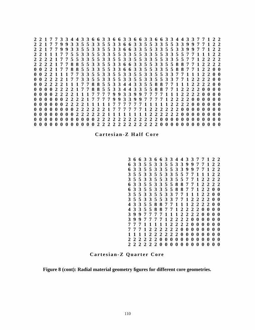
2 2 2 2 2 2 0 0 0 0 0 0 0 0 0 0 0 0
2 2 2 2 2 2 0 0 0 0 0 0 0 0 0 0 0 0
2 2 1 7 7 3 3 4 4 3 3 6 6 3 3 6 6 3 3 6 6 3 3 6 6 3 3 4 4 3 3 7 7 1 2 2 2 1 7 7 9 9 3 3 5 5 3 3 5 5 3 3 6 6 3 3 5 5 3 3 5 5 3 3 9 9 7 7 1 2 2 2 1 7 7 9 9 3 3 5 5 3 3 5 5 3 3 6 6 3 3 5 5 3 3 5 5 3 3 9 9 7 7 1 2 2 2 1 1 1 7 7 5 5 3 3 5 5 3 3 5 5 3 3 5 5 3 3 5 5 3 3 5 5 7 7 1 1 1 2 2 2 2 2 1 7 7 5 5 3 3 5 5 3 3 5 5 3 3 5 5 3 3 5 5 3 3 5 5 7 7 1 2 2 2 2 2 2 2 1 7 7 8 8 5 5 3 3 5 5 3 3 6 6 3 3 5 5 3 3 5 5 8 8 7 7 1 2 2 2 0 0 2 2 1 7 7 8 8 5 5 3 3 5 5 3 3 6 6 3 3 5 5 3 3 5 5 8 8 7 7 1 2 2 0 0 0 2 2 1 1 1 7 7 3 3 5 5 3 3 5 5 3 3 5 5 3 3 5 5 3 3 7 7 1 1 1 2 2 0 0 0 2 2 2 2 1 7 7 3 3 5 5 3 3 5 5 3 3 5 5 3 3 5 5 3 3 7 7 1 2 2 2 2 0 0 0 2 2 2 2 1 1 1 7 7 8 8 5 5 3 3 4 4 3 3 5 5 8 8 7 7 1 1 1 2 2 2 2 0 0 0 0 0 2 2 2 2 1 7 7 8 8 5 5 3 3 4 4 3 3 5 5 8 8 7 7 1 2 2 2 2 0 0 0 0 0 0 0 2 2 2 2 1 1 1 7 7 7 7 9 9 3 3 9 9 7 7 7 7 1 1 1 2 2 2 2 0 0 0 0 0 0 0 0 0 2 2 2 2 1 7 7 7 7 9 9 3 3 9 9 7 7 7 7 1 2 2 2 2 0 0 0 0 0 0 0 0 0 0 0 2 2 2 2 1 1 1 1 1 7 7 7 7 7 7 1 1 1 1 1 2 2 2 2 0 0 0 0 0 0 0 0 0 0 0 0 0 2 2 2 2 2 2 1 7 7 7 7 7 7 1 2 2 2 2 2 2 0 0 0 0 0 0 0 0 0 0 0 0 0 0 0 2 2 2 2 2 2 1 1 1 1 1 1 1 1 2 2 2 2 2 2 0 0 0 0 0 0 0 0 0 0 0 0 0 0 0 0 0 0 0 2 2 2 2 2 2 2 2 2 2 2 2 0 0 0 0 0 0 0 0 0 0 0 0 0 0 0 0 0 0 0 0 0 0 0 2 2 2 2 2 2 2 2 2 2 2 2 0 0 0 0 0 0 0 0 0 0 0
C a r t e s i a n - Z H a l f C o re
3 6 6 3 3 6 6 3 3 4 4 3 3 7 7 1 2 6 3 3 5 5 3 3 5 5 3 3 9 9 7 7 1 2 6 3 3 5 5 3 3 5 5 3 3 9 9 7 7 1 2 3 5 5 3 3 5 5 3 3 5 5 7 7 1 1 1 2 3 5 5 3 3 5 5 3 3 5 5 7 7 1 2 2 2 6 3 3 5 5 3 3 5 5 8 8 7 7 1 2 2 2 6 3 3 5 5 3 3 5 5 8 8 7 7 1 2 2 0 3 5 5 3 3 5 5 3 3 7 7 1 1 1 2 2 0 3 5 5 3 3 5 5 3 3 7 7 1 2 2 2 2 0 4 3 3 5 5 8 8 7 7 1 1 1 2 2 2 2 0 4 3 3 5 5 8 8 7 7 1 2 2 2 2 0 0 0 3 9 9 7 7 7 7 1 1 1 2 2 2 2 0 0 0 3 9 9 7 7 7 7 1 2 2 2 2 0 0 0 0 0 7 7 7 1 1 1 1 1 2 2 2 2 0 0 0 0 0 7 7 7 1 2 2 2 2 2 2 0 0 0 0 0 0 0 1 1 1 1 2 2 2 2 2 2 0 0 0 0 0 0 0 2 2 2 2 2 2 0 0 0 0 0 0 0 0 0 0 0 2 2 2 2 2 2 0 0 0 0 0 0 0 0 0 0 0
C a r t e s i a n - Z Q u a r t e r C o re
Figure 8 (cont): Radial material geometry figures for different core geometries.
110

0 0 0 0 5 5 5 0 0 0 0 0 5 5 5 5 5 5 5 5 5 5 0 0 5 5 5 5 4 4 4 5 5 5 5 0 0 5 5 5 4 4 4 4 4 4 5 5 5 0 5 5 5 4 4 4 1 4 1 4 4 4 5 5 5 5 5 4 4 4 4 3 3 3 3 4 4 4 4 5 5 5 5 4 4 1 3 3 3 3 3 3 3 1 4 4 5 5 0 5 4 4 4 3 3 2 3 3 2 3 3 4 4 4 5 0 0 5 5 4 1 3 3 3 3 3 3 3 3 3 1 4 5 5 0 0 5 5 4 4 3 3 3 3 3 3 3 3 3 3 4 4 5 5 00 5 5 5 4 4 3 2 3 3 3 3 3 2 3 4 4 5 5 5 0 0 5 5 4 4 3 3 3 3 3 3 3 3 3 3 4 4 5 5 0 0 5 5 4 1 3 3 3 3 3 3 3 3 3 1 4 5 5 0 0 5 4 4 4 3 3 2 3 3 2 3 3 4 4 4 5 0 5 5 4 4 1 3 3 3 3 3 3 3 1 4 4 5 5 5 5 4 4 4 4 3 3 3 3 4 4 4 4 5 5 5 5 5 4 4 4 1 4 1 4 4 4 5 5 5 0 5 5 5 4 4 4 4 4 4 5 5 5 0 0 5 5 5 5 4 4 4 5 5 5 5 0 0 5 5 5 5 5 5 5 5 5 5 0 0 0 0 0 5 5 5 0 0 0 0
Hexagonal-Z Full Core
0 5 5 5 4 4 3 2 3 3 3 0 5 5 4 4 3 3 3 3 3 3 0 5 5 4 1 3 3 3 3 3 3 0 5 4 4 4 3 3 2 3 3 2 5 5 4 4 1 3 3 3 3 3 3 5 5 4 4 4 4 3 3 3 3 4 5 5 5 4 4 4 1 4 1 4 4 0 5 5 5 4 4 4 4 4 4 5 0 5 5 5 5 4 4 4 5 5 5 0 5 5 5 5 5 5 5 5 5 5 0 0 0 0 5 5 5 0 0 0 0
Hexagonal-Z Third Core
33 3
3 3 32 3 3 2
3 3 3 3 34 3 3 3 3 4
4 4 1 4 1 4 45 4 4 4 4 4 4 5
5 5 5 4 4 4 5 5 55 5 5 5 5 5 5 5 5 5
0 0 0 0 5 5 5 0 0 0 0
Hexagonal-Z Sixth Core
Figure 8 (cont): Radial material geometry figures for different core geometries andsymmetries
111

IV.3. Cross-Section Data File
(Unit 3 => “XSECT” & Unit 33 => “AXSCIN”)
NG
Total number of energy groups.
NGT
Number of thermal energy groups.
ICOLXY
Total number of material colors (i.e. cross section sets).
NBUMAX
Maximum of the number of burnup mask values input for the cross-sections.
IF(NXSEC.EQ. “Y”) THEN READ
NPREC
Number of delayed neutron precursor groups.
NDECAY
Number of decay heat precursor groups.
NTERMMACRO,NTERMMACRI
Number of cross-section coefficients input for macroscopic cross-sections
w/o and w/ rods in.
NTERMCSCATRO,NTERMCSCATRI
Number of cross-section coefficients input for macroscopic scattering kernels
w/o and w/ rods in.
NTERMFPRO,NTERMFPRI
Number of cross-section coefficients input for transient fission products
microscopic absorption cross-sections w/o and w/ rods in.
[In following, IXSxxx values imply the following:
112

Base = 1,
Linear-Coolant Density (g/cm3) = 2,
Quadratic-Coolant Density (g/cm3) = 3,
Linear-Coolant Temperature (oF) = 4,
Linear in Square Root-Effect. Fuel Temperature (oF) = 5,
Linear-Soluble Poison Number Density (1/b) = 6,
Quadratic-Soluble Poison Number Density (1/b) = 7),
Cubic-Soluble Poison Number Density (1/b) = 8]
IF(NTERMMACRO.GT.0) READ
(IXSMACRO(ITERM),ITERM=1,NTERMMACRO)
Cross-section coefficients to be input for macroscopic cross-sections
w/o rods in.
IF(NTERMMACRI.GT.0) READ
(IXSMACRI(ITERM),ITERM=1,NTERMMACRI)
Cross-section coefficients to be input for macroscopic cross-sections
w/ rods in.
IF(NTERMCSCATRO.GT.0) READ
(IXSCSCATRO(ITERM),ITERM=1,NTERMCSCATRO)
Cross-section coefficients to be input for macroscopic scattering kernels
w/o rods in.
IF(NTERMCSCATRI.GT.0) READ
(IXSCSCATRI(ITERM),ITERM=1,NTERMCSCATRI)
Cross-section coefficients to be input for macroscopic scattering kernels
w/ rods in.
113

.
IF(NTERMFPRO.GT.0) READ
(IXSFPRO(ITERM),ITERM=1,NTERMFPRO)
Cross-section coefficients to be input for transient fission products
microscopic absorption cross-sections w/o rods in.
IF(NTERMFPRI.GT.0) READ
(IXSFPRI(ITERM),ITERM=1,NTERMFPRI)
Cross-section coefficients to be input for transient fission products
microscopic absorption cross-sections w/ rods in.
IMICRO (A5)
Microscopic cross-section option (“Y”/”N”).
IF(IMICRO.EQ. “Y”) THEN READ
INUMDEN (A5)
Node-wise isotopic number densities available (“Y” / “N”).
IF (INUMDEN.EQ. “Y”) THEN READ
FNUMDEN (A40)
Name of the file containing the node-wise initial isotopic number densities
NTERMMICRO
Number of cross-section coefficients input for microscopic cross-sections
w/o rods in.
NTERMMICRI
Number of cross-section coefficients input for microscopic cross-sections
w/ rods in.
IF(NTERMMICRO.GT.0) READ
(IXSMICRO(ITERM),ITERM=1,NTERMMICRO)
114
functionutronnctioned
cursor
utron
Cross-section coefficients to be input for microscopic cross-sections
w/o rods in.
IF(NTERMMICRI.GT.0) READ
(IXSMICRI(ITERM),ITERM=1,NTERMMICRI)
Cross-section coefficients to be input for microscopic cross-sections
w/ rods in.
ENDIF IMICRO
ENDIF NXSEC
AXSEC (A5)
Cross-section colors are read from different input files (“Y”/ “N”).
IF(NXSEC.EQ. “Y”) THEN READ
RLI,RLX,RLPM
Decay constants (I-135, Xe-135, Pm-149) (1/sec)
The next data, the delayed neutron precursor decay constants, can be entered as aof both isotope and delayed neutron precursor group or as a function of delayed neprecursor group only. To enter the delayed neutron precursor decay constants as a fuof both isotope and precursor group, write “ALAMDAMI” in a line preceding the delayneutron precursor decay constants input (see example below).
Delayed neutron precursor decay constants as a function of delayed neutron pregroup only:
(ALAMDA(I),I=1,NPREC)
Delayed neutron precursor decay constants (1/sec).
Delayed neutron precursor decay constants as a function of both delayed neprecursor group and isotope:
ALAMDAMI (mandatory card of format A8)
DO ISOT=1,8...For each isotope
(ALAMDAMIC(ISOT,IPREC), IPREC=1,NPREC)
115

42.
Isotopic dependent delayed neutron precursor decay constants (1/sec).
ENDDO ISOT
Note: ISOT value corresponds to the following isotope:
1=U-234, 2=U-235, 3=U-236, 4=U-238, 5=Pu-239, 6=Pu-240, 7=Pu-241, 8=Pu-2
DO IG=1,NG...For each energy group
(XHIDMI(IG,IPREC),IPREC=1,NPREC)
Delayed neutron fission spectrum.
ENDDO IG ...Energy loop
(ZETA(I),I=1,NDECAY)
Decay heat precursors decay rates (1/sec).
IF(IMICRO.EQ. “Y”) THEN
DO ISOT=1,NISOT... For each isotope (U-234, U-235, U-236, U-238,
Pu-239, Pu-240, Pu-241, Pu-242)
(BETAMI(ISOT,IPREC),IPREC=1,NPREC)
Delayed neutron yields for isotope.
ENDDO ISOT...Isotope loop
DO IG=1,NG...For each energy group
(XHIPMI(ISOT,IG),ISOT=1,9)
Prompt neutron spectra for each isotope ISOT
(1=U-234, 2=U-235, 3=U-236, 4=U-238,
5=Pu-239, 6=Pu-240, 7=Pu-241, 8=Pu-242, 9=Am-241)
ENDDO IG...Energy loop
DO ISOT=1,NISOT... For each isotope (U-234, U-235, U-236, U-238,
Pu-239, Pu-240, Pu-241, Pu-242)
116

).
Am-
(ALPHAI(ISOT,IDECH),IDECH=1,NDECAY)
Decay heat group yields for isotope.
ENDDO ISOT...Isotope loop
DO ISOT=1,NISOT... For each isotope (U-234, U-235, U-236, U-238,
Pu-239, Pu-240, Pu-241, Pu-242)
GINMI(ISOT),GXNMI(ISOT),GPNMI(ISOT)
Transient fission product yields (I135, Xe135, Pm149) for isotope.
ENDDO ISOT...Isotope loop
DO IG=1,NG...For each energy group
RNUU4(IG),RNUU5(IG),RNUU6(IG)
Nu values for isotopes (U-234, U-235, U-236).
RNUU8(IG),RNUP9(IG),RNUP0(IG),RNUP1(IG),RNUP2(IG),RNUA1(IG)
Nu values for isotopes (U-238, Pu-239, Pu-240, Pu-241, Pu-242, Am-241
ENDDO IG...Energy group loop
RKU34, RKU35, RKU36
Kappa values (Mev) for isotopes (U-234, U-235, U-236).
RKU38, RKPU39, RKPU40, RKPU41, RKPU42, RKAM41
Kappa values (Mev) for isotopes (U-238, Pu-239, Pu-240, Pu-241, Pu-242,
241).
GLFP1,GLFP2
Lumped fission products 1 and 2 yields.
ENDIF IMICRO
ENDIF NXSEC
NFUEXY
Number of non-fuel material colors.
117

L
Cross section table sets input follow.
Units: Macroscopic cross section (1/cm), microscopic cross sections (barns),
burnup (MWD/MTM)
DO ICOL=1,ICOLXY ...For each material color
Note ‘I’ used below is determined from ICOL and denotes internal storage index of ICOth
material color entry.
IF(AXSEC.EQ. “Y”) READ
AXSCIN (A40)
Name of file containing cross-sections for a specific color.
Following input on file name “XSECT” if AXSEC = “N” and on file name “AXSCIN” if AXSEC =
“Y”.
Header Line (A80)
NESTLE does not utilize-to help with data file preparation.
Header Line (A80)
NESTLE does not utilize-to help with data file preparation.
AFUEL (A5)
Material cross-sections now to be entered corresponds to a fuel
(i.e. fissionable) (“Y”/”N”).
NCOLOR(I)
Material color number of cross-sections to be entered.
118

n
IF(AFUEL.EQ. “Y”) READ
NMAX(I)
Number of burnup steps for fuel material color that cross sections
provided at. [For non-fuels set equal to 1.]
WTFRRO(I), WTFRRI(I), FUFR(I)
Volume fractions for coolant w/o rods, coolant w/ rods, and fuel.
RHOWREF(I), TCOLREF(I), TFREF(I), REFB(I)
Reference conditions cross-sections evaluated at: coolant density (lbm/ft3),
coolant temperature (oF), fuel effective temperature (oF), and reference soluble boro
concentration (ppm).
(BUBOS(N,I),N=1,NMAX(I))
Burnup values the cross-sections are input at.
DO ITERM=1,NTERMMACRO ...For each cross-section coefficient
DO N=1,NMAX(I) ...For each burnup step
DO IG=1,NG...For each energy group
(XSECRO(N,I,IRX,IG,ITERM),IRX=1,NRXMAX)
Macroscopic cross sections coefficients w/o rods:
IMICRO= “Y”: transport, absorption.
IMICRO= “N”: transport, absorption, nu-fission, kappa-fission, nu.
ENDDO IG...Energy group loop
ENDDO N...Burnup step loop
ENDDO ITERM ...Cross-section coefficient loop
DO ITERM=1,NTERMCSCATRO ...For each cross-section coefficient
DO N=1,NMAX(I) ...For each burnup step
DO IG=1,NG...For each energy group
119

(XSECSCRO(N,I,IG,IGP,ITERM),IGP=1,NG-1)
Scattering transfer macroscopic cross sections coefficients w/o rods;
from group igp (or igp+1 when upscatter) to group ig.
(Note within group (ig to ig) scattering is not entered, hence the
non-square matrix.
ENDDO IG...Energy group loop
ENDDO N...Burnup step loop
ENDDO ITERM ...Cross-section coefficient loop
IF(NXSEC.EQ. “Y”) THEN READ
DO ITERM=1,NTERMCSCATRI ...For each cross-section coefficient
DO N=1,NMAX(I). ..For each burnup step
DO IG=1,NG...For each energy group
(XSECRI(N,I,IRX,IG,ITERM),IRX=1,NRXMAX)
Macroscopic cross sections coefficients w/ rods:
IMICRO= “Y”: transport, absorption.
IMICRO= “N”: transport, absorption, nu-fission, kappa-fission, nu.
ENDDO IG...Energy group loop
ENDDO N...Burnup step loop
ENDDO ITERM ...Cross-section coefficient loop
DO ITERM=1,NTERMMACRI ...For each cross-section coefficient
DO N=1,NMAX(I) ...For each burnup step
DO IG=1,NG...For each energy group
(XSECSCRI(N,I,IG,IGP,ITERM),IGP=1,NG-1)
Scattering transfer macroscopic cross sections coefficients
w/ rods; from group igp (or igp+1 when upscatter) to group ig.
120

(Note within group (ig to ig) scattering is not entered, hence the
non-square matrix.
ENDDO IG...Energy group loop
ENDDO N...Burnup step loop
ENDDO ITERM ...Cross-section coefficient loop
ENDIF NXSEC
DO N=1,NMAX(I) ...For each burnup step
DO IG=1,NG...For each energy group
B2COL(N,I,IG)
Buckling (1/cm2) Normally input as 0’s for 3D geometries.
ENDDO IG...Energy group loop
ENDDO N...Burnup step loop
IF (AFUEL.EQ. “Y”) THEN READ
DO N=1,NMAX(I) ...For each burnup step
(XHIPN(N,I,IG),IG=1,NG)
Prompt fission neutron spectrum
ENDDO N...Burnup step loop
ENDIF AFUEL
DO N=1,NMAX(I) ...For each burnup step.
DO IG=1,NG...For each energy group
(ADFS(I,N,IADF,IG),IADF=1,NADFS)
Assembly Discontinuity Factors w/o rods:
(Cartesian (NADFS=6): N, E, S,W, UP, DOWN)
(Hexagonal (NADFS=8): NE, E, SE, SW, W, NW, UP, DOWN)
ENDDO IG...Energy group loop
121
tive
unit
ENDDO N...Burnup step loop
IF(NXSEC.EQ. “Y”) THEN READ
DO N=1,NMAX(I) ...For each burnup step
DO IG=1,NG...For each energy group
(ADFSRD(I,N,IADF,IG),IADF=1,NADFS)
Assembly Discontinuity Factors w/ rods:
(Cartesian (NADFS=6): N, E, S, W, UP, DOWN)
(Hexagonal (NADFS=8): NE, E, SE, SW, W, NW, UP, DOWN)
ENDDO IG...Energy group loop
ENDDO N...Burnup step loop
IF(IMICRO.EQ. “N”) THEN READ
DO N=1,NMAX(I). ..For each burnup step
(VELOCN(N,I,IG),IG=1,NG)
Neutron velocity (cm/sec).
ENDDO N...Burnup step loop
ELSEIF (IMICRO.EQ. “Y”) THEN READ
DO N=1,NMAX(I). ..For each burnup step
(VELOCN(N,I,IG),IG=1,NG), (BFACT(N,I,IPREC),IPREC=1,NPREC)
Neutron velocity (cm/sec), the delayed neutron importance.
The delayed neutron importance is defined as the ratio of the effec
delayed neutron yields over the delayed neutron yields from lattice
assembly depletion: ,
where
ENDDO N...Burnup step loop
βeff β BFACT×=
β βisot νΣ f g
isotφgg 1=
G
∑isot=1
# fiss. isot.
∑
νΣ f g
isotφgg 1=
G
∑isot=1
# fiss. isot.
∑
⁄=
122

ENDIF ... IMICRO
IF (AFUEL.EQ. “Y”) THEN READ
DO ITERM=1,NTERMFPRO ...For each cross-section coefficient
DO N=1,NMAX(I) ...For each burnup step
DO IG=1,NG...For each energy group
(XFPNRO(N,I,IG,IFP,ITERM),IFP=1,2)
Microscopic absorption cross-sections coefficients w/o
rods: (Sm149, Xe135)
ENDDO IG ...Energy group loop
ENDDO N...Burnup step loop
ENDDO ITERM ...Cross-section coefficient loop
DO ITERM=1,NTERMFPRI ...For each cross-section coefficient
DO N=1,NMAX(I) ...For each burnup step
DO IG=1,NG...For each energy group
(XFPNRI(N,I,IG,IFP,ITERM),IFP=1,2)
Microscopic absorption cross-sections coefficients
w/ rods: (Sm-149, Xe-135)
ENDDO IG ...Energy group loop
ENDDO N...Burnup step loop
ENDDO ITERM ...Cross-section coefficient loop
IF(IMICRO.EQ. “N”) THEN READ
DO N=1,NMAX(I) ...For each burnup step
GIN(N,I),GXN(N,I),GPN(N,I)
Transient fission products yields (I135, Xe135, Pm149).
ENDDO N...Burnup step loop
123

DO N=1,NMAX(I) ...For each burnup step
(BETAN(N,I,IPREC),IPREC=1,NPREC)
Delayed neutron yields.
ENDDO N...Burnup step loop
DO N=1,NMAX(I) ...For each burnup step
(ALPHAN(N,I,IDECH),IDECH=1,NDECAY)
Decay heat group yields.
ENDDO N...Burnup step loop
ENDIF IMICRO
ENDIF AFUEL
ENDIF NXSEC
IF(NXSEC.EQ. “Y”) THEN READ
IF (AFUEL.EQ. “Y”) THEN READ
IF(IMICRO.EQ. “Y”) THEN READ
Number densities of isotopes in following order (nuclei/cm3x10-24):
(UPUDEN(I,IRX),IRX=1,3)
(U234, U235, U236)
(UPUDEN(I,IRX),IRX=4,8)
U238, Pu239, Pu240, Pu241, Pu242)
(UPUDEN(I,IRX),IRX=9,10)
(Lumped FP#1, Lumped FP#2)
(UPUDEN(I,IRX),IRX=11,12)
(Burnable Poison, Am-241)
DO N=2,NMAX(I) ... For each burnup step
Number densities of isotopes at other burnup steps (nuclei/cm3x10-24):
124
(INITND(I,N,IRX),IRX=1,4)
(U234, U235, U236, U238)
(INITND(I,N,IRX),IRX=5,8)
(Pu239, Pu240, Pu241, Pu242)
(INITND(I,N,IRX),IRX=11,12)
(Burnable Poison, Am-241)
ENDDO N
DO ITERM=1,NTERMMICRO ...For each cross-section coefficient
DO N=1,NMAX(I). ..For each burnup step
DO IG=1,NG...For each energy group
(UCHAINRO(N,I,IRX,IG,ITERM),IRX=1,6)
(UCHAINRO(N,I,IRX,IG,ITERM),IRX=7,12)
(UCHAINRO(N,I,IRX,IG,ITERM),IRX=13,16 and IRX=20,21)
Microscopic cross sections coefficients w/o rods:
(absorption, fission) for each isotope:
1st line (U-234, U-235, U-236)
2nd line (U-238, Pu-239, Pu-240)
3rd line (Pu-241, Pu-242, Am-241)
(UCHAINRO(N,I,IRX,IG,ITERM),IRX=17,18)
Microscopic absorption cross sections coefficients w/o
rods: Lumped FP#1, Lumped FP#2
UCHAINRO(N,I,19,IG,ITERM)
Microscopic absorption cross sections coefficients w/o
rods: Burnable Poison
ENDDO IG...Energy group loop
125

ENDDO N...Burnup step loop
ENDDO ITERM ...Cross-section coefficient loop
DO ITERM=1,NTERMMICRI ...For each cross-section coefficient
DO N=1,NMAX(I). ..For each burnup step
DO IG=1,NG...For each energy group
(UCHAINRI(N,I,IRX,IG,ITERM),IRX=1,6)
(UCHAINRI(N,I,IRX,IG,ITERM),IRX=7,12)
(UCHAINRI(N,I,IRX,IG,ITERM),IRX=13,16 and IRX=20,21)
Microscopic cross sections coefficients w/ rods:
(absorption, fission) for each isotope:
1st line (U-234, U-235, U-236)
2nd line (U-238, Pu-239, Pu-240)
3rd line (Pu-241, Pu-242, Am-241)
(UCHAINRI(N,I,IRX,IG,ITERM),IRX=17,18)
Microscopic absorption cross sections coefficients w/
rods: Lumped FP#1, Lumped FP#2
UCHAINRI(N,I,19,IG,ITERM)
Microscopic absorption cross sections coefficients w/
rods: Burnable Poison
ENDDO IG...Energy group loop
ENDDO N...Burnup step loop
ENDDO ITERM ...Cross-section coefficient loop
ENDIF IMICRO
ENDIF AFUEL
ENDIF NXSEC
126

ure.
End of input on file name “AXSCIN” if AXSEC = “Y” & returning to file name “XSECT”.
ENDDO I...Material color loop
Remaining input on file name “XSECT”.
Blank Line
IF (NXSEC.EQ. “Y”) THEN READ
NFRODS
Number of fuel rods per bundle (assembly)
FUELRAD
Fuel rod radius (in)
WC,WP
Fuel temperature rise and average fuel temperature Doppler effective fuel
temperature weight factors.
NPOLTAF
Order of polynomial fitting average fuel temperature versus linear power density.
(COF_TAF(I),I=0,NPOLTAF-1)
Fitting coefficients for average fuel temperature (oF) versus
linear power density (kw/ft).
NPOLHFF
Order of polynomial fitting effective heat transfer coefficient versus fuel temperat
(COF_HFF(I),I=0,NPOLHFF-1)
Fitting coefficients for effective heat transfer coefficient (kw/ft2-oF) versus
fuel temperature (oF).
NPOLTSF
Order of polynomial fitting surface fuel temperature versus linear power density.
(COF_TSF(I),I=0,NPOLTSF-1)
127

Fitting coefficients for surface fuel temperature (oF) versus
linear power density (kw/ft).
MOLW_COL
Molecular weight of coolant.
ATMW_SOLP
Atomic weight of soluble poison.
ABUN_SOLP
a/o of absorbing isotope of soluble poison (e.g.B-10).
PIN
Coolant pressure (psia). Only use within NESTLE is for editing.
TCOLSAT,UCOLG,RHOG
Coolant saturation temperature (oF), saturated vapor internal energy (BTU/lbm)
and saturated vapor density (lbm/ft3).
DEPF
Fraction of fission energy deposited directly within fuel.
TCOLIN
Coolant inlet temperature (oF). Only used for non-transient problems.
TCOLMIN,TCOLMAX
Coolant inlet temperature (oF) search range for criticality or power level search.
GMASS
Coolant mass velocity (lb/hr-ft2). Only used for non-transient problems.
GMASS > 0 => Inlet mass velocity entering bottom fuel node, implying
cross-sectional flow rate = fuel node wet fraction X node x-y plane area.
GMASS < 0 => Inlet mass velocity below bottom axial node, implying
cross-sectional flow area = node x-y plane area.
128

NPOLUCOL
Order of polynomial fitting coolant liquid internal energy versus temperature.
(COF_UCOL(I),I=0,NPOLUCOL-1)
Fitting coefficients for coolant internal energy (BTU/lbm) versus temperature (oF).
NPOLTCOL
Order of polynomial fitting coolant liquid temperature versus internal energy.
(COF_TCOL(I),I=0,NPOLTCOL-1)
Fitting coefficients for coolant liquid temperature (oF) versus internal energy
(BTU/lbm).
NPOLRHOWC
Order of polynomial fitting coolant liquid density versus internal energy.
(COF_RHOWC(I),I=0,NPOLRHOWC-1)
Fitting coefficients for coolant liquid density (lbm/ft3) versus internal energy
(BTU/lbm).
NPOLCPF
Order of polynomial fitting fuel specific heat versus temperature.
(COF_CPF(I),I=0,NPOLCPF-1)
Fitting coefficients for fuel specific heat (BTU/lbm-oF) versus temperature (oF).
RHOWTF
Fuel density (lbm/ft3).
RATIOHMFUEL
Ratio of heavy metal density to fuel material density.
(Used to convert MTM to MT fuel material)
QQT
Core power density at rated full power (kw/liter).
129

ENDIF NXSEC
(RT(IG),IG=1,NG)
Initial estimates of relative group flux values.
(SEXT(IG),IG=1,NG)
External source strengths (1/cm3-sec).
130

IV.4. Kinetic Data File
(Unit 4 => “KINET”)
IF (ITRAN.EQ. “Y”) THEN READ
NPERT
Number of times that time-dependent input parameters are provided.
NPRINT
Number of times that time-dependent output is to be printed.
NTSPN
Total number of time spans, each utilizing a constant time step size over the
time span.
ENDDO ITRAN
IF (IXE.EQ.4 OR IXE.EQ.5) THEN READ
NFP
Number of time-steps for transient fission product case.
ENDIF IXE
IF(ITRAN.EQ. “Y”)THEN READ
DO IT=1,NPERT...For each transient time perturbation
TIMETR(IT),PMT(IT),TINT(IT),GMINT(IT)
Time (sec), soluble poison concentration (PPM), coolant inlet temperature (oF),
coolant mass flow rate (lb/ft2-sec) (4 values per line)
TIMETR(IT),(ZPT(IBK,IT), IBK=1,NBACU)
Time (sec), control banks steps withdrawn (1+NBACU values per line)
[Note TIMETR(1) must equal 0.]
ENDDO...Transient time perturbation loop
(TIMEPR(IT),IT=1,NPRINT)
131

Time (sec) output is to be printed.
(TIMESP(IT),DELT(IT),IT=1,NTSPN)
Use time step size DELT(IT) (sec) from time TIMESP(IT-1) to TIMESP(IT) (sec)
where TIMESP(0) = 0.
ENDDO ITRAN
IF (IXE.EQ.4 ORIXE.EQ. 5) THEN READ
DO IFP=1,NFP...For each fission product transient time perturbation
TIMEFP(IFP),PRFP(IFP),PMFP(IFP),TINFP(IFP)
Time (hrs), core power (relative), soluble poison (PPM),
coolant inlet temperature (oF).
[Note that if IBOR=”Y” the parameter being searched upon will overwrite the
input value of this parameter.]
TIMEFP(IFP),(ZBFP(IBK,IFP),IBK=1,NBACU)
Time (hrs), Control banks steps withdrawn (1+NBACU values per line)
[Note that if IBOR=”Y” the parameter being searched upon will overwrite the
input value of this parameter.]
ENDDO...Fission product transient time perturbation loop
ENDIF IXE
132

ion
IV.5. Solution Method Control Data File
(Unit 5 => “PERFM”)
N_THRMITR
Maximum number of thermal scattering iterations.
KITR
Maximum number of outer iterations.
EPSK
Outer iteration stopping criteria on eigenvalue
EPSOT
Outer iteration stopping criteria on L2 norm of relative residual of the outer iterative
equation
EPSRESID
Outer iteration stopping criteria on L2 norm of relative residual of the diffusion equat
EPSINF
Outer iteration stopping criteria on Linf norm of relative fission source error (Chebyshev
acceleration) or outer iterative equation (Weilandt Shift)
EPSDET
Inner iteration convergence criteria on L2 relative error reduction
ACONV (A5)
Stopping criteria required to be satisfied after a coefficient matrix update (“Y”/ “N”)
AMETHOD (A5)
Solution method (“FDM”/ “NEM”)
IF (AMETHOD.EQ. “NEM”) THEN READ
NNEM
Maximum number of iterations between NEM coupling coefficients’ updates
133

T-H Off: Number of outer iterations/update
T-H On: Number of T-H calls/update
EPSNEM
Outer iteration L2 relative error reduction criteria used for determining when NEM
coupling coefficients’ updates are to be completed
ENDIF AMETHOD
IF (IBURN.EQ. “Y”) THEN READ
ADEPL
Depletion method: Predictor or Predictor-Corrector (“PRED”/”CORR”)
IF(ADEPL.EQ. “CORR”) THEN READ
NDELPC
Frequency of Corrector updates for Predictor-Corrector method
T-H Off: Number of outer iteration/update
T-H On: Number of T-H calls/update
ENDIF ADEPL
ENDIF IBURN
AOUTER (A5)
Chebyshev acceleration on (“CHEB”)
Weilandt Shift acceleration on (“WEIL”)
IUPCHE,EPREDRESID
Upper limit on Chebyshev order or Weilandt Shift cycle, reduction of L2 relative
residual error for the diffusion equation from starting new Chebyshev order or
Weilandt Shift cycle
IF(AOUTER.EQ. “WEIL”) THEN READ
IF(ITRAN.EQ. “Y”.OR.IADJ.EQ. “Y”) THEN READ
134

WEILANDTEI,WEILANDTFS
Forward eigenvalue or steady-state and transient or adjoint upper limit on
Weilandt shift with respect tok-1
ELSE READ
WEILANDTEI
Forward eigenvalue or steady-state upper limit on Weilandt shift with respect tok-1
ENDIF ITRAN
OMEGAEXT
Stationary extrapolation parameter for the flux
ENDIF AOUTER
AISC (A5)
Steady-state scaling factor acceleration on (“Y”/”N”)
IF (AISC.EQ. “Y”) THEN READ
ISC
Outer iteration when steady-state scaling factor acceleration first applied.
ASPSH (A5)
Steady-state spectral shift correction on (“Y”/”N”)
ENDIF AISC
IF (ITRAN.EQ. “Y”) THEN READ
IONE
Number of outer iterations per time step control logic.
Convergence criteria controled=1
Fixed number=2
IF (IONE.EQ.2) THEN READ
IOK
135

Number of outer iterations per time step.
ENDIF IONE
ANFDBKIMP (A5)
Implicit (versus explicit) thermal-hydraulics to be used for transients (“Y”/”N”)
AISCTR (A5)
Transient scaling factor acceleration on (“Y”/ “N”)
IF (AISCTR.EQ. “Y”) THEN READ
ISCTR
Outer iteration when transient scaling factor acceleration first applied.
ASPSHTR
Transient spectral shift correction on (“Y”/”N”)
ENDIF AISCTR
ENDIF ITRAN
136

be
IV.6. Initial Exposure Data File
(Unit 79=> “FINITEXP”)
Line 1: TITLE
Line 2:Blank or comment line
Line 3: NNODE
Number of nodes whose axially-dependent exposure values are provided.
To minimize the length of the input file, input for fresh nodes (exposure=0.0) can
skipped.
Line 4:Blank or comment line
Line 5:Blank or comment line
DO IY=1, NY ... for each y mesh
(NODEID(IY,IX),IX=NXSTART(IY),NXEND(IY),NXSKIP)
Node ID number as a function of x- and y-mesh number.
See Section IV.2 for the meaning of NY, NXSTART(IY), NXEND(IY), and
NXSKIP.
ENDDO
Line 6+NY: Blank or comment line
DO I=1,NNODE ... for each node
INODE
Node ID number
(EXP(INODE,IZ),IZ=IZCOLS,IZCOLE)
Node exposure (MWd/MTU).
See Section IV.2 for the meaning of IZCOLS and IZCOLE.
ENDDO
137

gonal
(see
The following input data are needed for hexagonal assembly calculation only:
INITSUREXP (A5)
Option to provide the initial surface exposure values on the six surfaces of each hexa
assembly (“Y”/ “N”).
If the initial surface exposure input is not available, then the burnup gradient treatment
Section II.4.b) will not be completed.
The following is the format for the initial surface exposure input (if desired).
IF (INITSUREXP.EQ. “Y”) THEN READ
DO I=1,NNODE
((BUSURF(INODE,IZ),IZ=IZCOLS,IZCOLE),ISURF=1,6)
Surface exposure value (MWd/MTU).
ISURF corresponds to the following hexagonal surface:
West =1 , East =2, Northwest=3, Southeast=4, Northeast=5, Northwest=6
See Section IV.2 for the meaning of IZCOLS and IZCOLE.
ENDDO
ENDIF
138

139
IV.7. Initial Isotopic Number Densities Data File
(Unit 77=> “FNUMDEN”)
Line 1: TITLE
Line 2:Blank or comment line
Line 3: NNODE
Number of nodes whose axially-dependent exposure values are provided.
To minimize the length of the input file, input for fresh nodes (exposure=0.0) can be
skipped.
Line 4:Blank or comment line
Line 5:Blank or comment line
DO IY=1, NY ... for each y mesh
(NODEID(IY,IX),IX=NXSTART(IY),NXEND(IY),NXSKIP)
Node ID number as a function of x- and y-mesh number.
See Section IV.2 for the meaning of NY, NXSTART(IY), NXEND(IY), and
NXSKIP.
ENDDO
Line 6+NY: Blank or comment line
DO I=1,NNODE... for each node
INODE
Node ID number
DO IZ=IZCOLS,IZCOLE ... for each z mesh in the fuel region
(ANUMDEN(INODE,IZ,ISOT),ISOT=1,13)
Isotopic number densities.
ISOT=1 -> U234, ISOT=2 -> U235, ISOT=3 -> U236, ISOT=4 -> U238,
ISOT=5 -> Pu239, ISOT=6 -> Pu240, ISOT=7 -> Pu241, ISOT=8 -> Pu242,
ISOT=9 -> LFP1, ISOT=10 -> LFP2, ISOT=11 -> DBP, ISOT=12 -> Am241,
ISOT=13 -> Sm
See Section IV.2 for the meaning of IZCOLS and IZCOLE.
ENDDO

ed.
find
IV.8. Pin-Power Data File
(Unit 81=> “INPPIN”)
Note: pin power reconstruction option is available for Hexagonal geometry only.
IF (PPR.EQ. “Y”.and. FPIN.EQ. “Y”) THEN READ
NINP
Number of corner point & form factor data set to be input
NPIN
Number of form factor data provided within a hexagonal fuel assembly.
DO IPIN=1,NPIN ... For each pin
PINLOCX(IPIN), PINLOCY(IPIN)
The x- and y-coordinate of the center of the fuel pin where the form factor is provid
ENDDO IPIN
DO IDATA=1,NINP ...For each node
NCOLTEMP
Material number color of pin-power data to be entered. NESTLE code will then
the index I where NCOLOR(I)1 = NCOLTEMP
DO N=1,NMAX(I) 2...For each burnup
DO IG=1,NG...For each neutron energy group
(CPADF(I,N,IADF,IG),IADF=1,6)
Corner Point Assembly Discontinuity Factors w/o rods
ENDDO IG
1. See Section IV.32. See Section IV.3
1
3
26
5
4Location of Corner Point Discontinuity Factor
140

ENDDO N
IF (NXSEC1.EQ. “Y”) THEN
DO N=1,NMAX(I) ... For each burnup step
(CPADFRD(I,N,IADF,IG),IADF=1,6)
Corner Point Assembly Discontinuity Factors with rods
ENDDO N
ENDIF NXSEC
DO N=1,NMAX(I) ...For each burnup step
(FF(I,N,IPIN),IPIN=1,NPIN)
Pin-wise form factor without rods.
ENDDO N
IF (NXSEC.EQ. “Y”) then
DO N=1,NMAX(I)
(FFRD(I,N,IPIN),IPIN=1,NPIN)
Pin-wise form factor with rods.
ENDDO N
ENDIF NXSEC
ENDDO IDATA
ENDIF PPR
1. See Section IV.1
141

that
sed
ures
g to
king.
ption
the
d with
nsient
of the
ction, a
e the
here
each
long
cific
he
V. Programmer’s Guide
This section presents information about the organization and coding of NESTLE
should prove useful to individuals who wish to understand and modify the officially relea
version of NESTLE. Since NESTLE contains over 26,000 lines of FORTRAN, 132 proced
(i.e. subroutines, main program and function subprograms) and 69 fcb files (i.e. files containing
one or more named COMMON blocks referred to in INCLUDE statements), those wishin
understand the code structure should be prepared to commit significant time to this underta
V.1. Dependence Diagram
The dependence diagram for the NESTLE code is shown in Figure (9). With the exce
of the main program, in Figure (9) the subroutines are listed alphabetically indicating
subroutines called one-level deep. Four main control paths exist within the code, associate
the solution of the eigenvalue and steady-state external source, eigenvalue adjoint, tra
fission product, and transient neutronics problems. These main control paths utilize many
same procedures. Where different subroutines are required to perform nearly the same fun
suffix at the end of the subroutine name is utilized to distinguish the function. For exampl
suffixes ‘k’ (or ‘tr’ ), ‘ss’ and ‘ad’ refer to respectivelykinetic (or transient),steady-state, and
adjoint; and, the suffixes ‘c’ and ‘h’ refer to respectivelyCartesian andHexagonal geometries.
V.2. Summary of Procedures
As noted above, there are a total of 132 procedures incorporated into NESTLE. T
names and a brief description of their functions are given in Table (5). The header of
procedure contains a brief description via COMMENT lines. Most procedures have very
calling argument lists which are required to allow variables to have problem spe
dimensionality without recompilation. This point will be further explained below in t
142

ronic
code
s. To
that
able’s
bles’
dated
ilizing
ere
buted
ocks
s
In this
iring
for
if an
ear for
by a
he
subsection entitle Variables’ Storage.
V.3. Variables’ Definitions
Rather than define variables throughout the source code of NESTLE, an elect
dictionary has been created. The electronic dictionary consists of the FORTRAN
NESTLE.DICT and the associated data base containing variables’ names and definition
determine the definition of a variable, the user initiates execution of NESTLE.DICT, indicates
a definition is sought, and enters the variable name. NESTLE.DICT then outputs the vari
definition. This is all done in an interactive manner. Options also exist to add and delete varia
names and definitions. At the conclusion of the NESTLE.DICT execution the data base is up
reflecting any changes made, if so desired. Table (7) shows an interactive session ut
NESTLE.DICT. It is most conveniently used by opening a separate window wh
NESTLE.DICT will be controlled from. This code and the associated data base are distri
with the NESTLE code.
V.4. Variables’ Storage
Variables with dimensionality are stored either in a container array or in common bl
of fixed dimensionality. The container array (i.e. A Array) stores all variables whose dimension
are problem specific, such as number of energy groups and number of spatial nodes.
manner the dimensionality of variables can be specified at run-time without requ
recompilation for problems with different dimensionality. Also memory is only allocated
variables that will be employed for the specific problem as specified via input. For example,
eigenvalue problem is to be solved no memory space is allocated for variables that only app
a neutronics transient problem. The A array is specified (including its size indicated
PARAMETER statement) in named COMMON block ‘array’ stored in file ‘array.fcb’. T
143

INE
format
or.
b’
r (
MON
clude
N
ment
e fcb
de’
ming
the
d to
ction
E’ is
call
the
rent
starting address of all variables stored in the A array are determined in SUBROUT
POINTER. The variable names associated with the starting addresses all have the
‘LXXXN’ where ‘XXX’ is the name of the variable that the starting address is being given f
The named COMMON block ‘varlen’ stored in file ‘varlen.fcb’ and varlens in file ‘varlens.fc
contain all the pointer variables.
As noted above, COMMON blocks are utilized to store variables that are either scalai.e.
have no dimensionality) or have problem independent dimensionality. These named COM
blocks are incorporated into the source code via the ‘include’ statement using the format ‘in
yyy.fcb’ where ‘yyy.fcb’ is the file name of a file containing one or more named COMMO
blocks. A listing of the fcb files is presented in Table (6). The advantage of the ‘include’ state
is that modifications to a COMMON block need only be made in one place, the appropriat
file. The danger when using the UNIX ‘make’ feature is that not all procedures which ‘inclu
the altered fcb file will be recompiled since they have not been ‘touched’. A sound program
practice when altering fcb files is to ‘grep’ on *.f files the fcb file names altered and ‘touch’ all
procedures containing the altered fcb files.
V.5. Machine Specific Instructions
The only machine specific instruction that is utilized by NESTE is the clock call use
provide timing information that is output. Rather than have the machine specific clock instru
scattered throughout the source code, a function subroutine named ‘FUNCTION GTIM
called. Within this subroutine are the machine specific clock calls. Currently the clock
instructions for DEC ULTRIX, IBM AIX and SUN OS operating systems are included, with
clock calls not utilized commented out. In this manner NESTLE can be ported to diffe
platforms and only the file gtime.f needs to be modified.
144

, the
ted in
dial
a
-Z
when
h the
urface
n
dition
index,
de is
tside
the
tive
just
aries
and y
. The
l.
s by
V.6. Geometry Treatment
Since both Cartesian-Z and Hexagonal-Z geometry can be treated by NESTLE
geometry treatment needs to be fairly flexible. Most of the setup of the geometry is comple
SUBROUTINE GEOMETRY. For most variables the indices associated with the two ra
directions (IX,IY) are rolled into a single index (IXY) indirectly indexed vi
IXY=NDNUM(IX,IY). This greatly facilitates handling both Cartesian-Z and Hexagonal
geometries. In addition, no memory is wasted to store variables outside the solution domain
a ‘raggedy edge’ solution domain is employed. In addition to the nodes associated wit
solution domain, an extra layer of nodes is added radially about the core such that every s
associated with either an interior boundary (i.e. symmetry boundary) or exterior boundary has a
extra node located across the surface. This is done to facilitate the various boundary con
treatments. Since these extra nodes IXY index starts after the solution domain nodes IXY
they can be easily recognized by the value of IXY. In this manner whether a neighbor no
within the solution domain can be determined. If it is determined that the neighbor node is ou
the solution domain, than a vector NBC(IXY) contains the information required to apply
specified boundary condition. For cyclic boundary conditions, NBC(IXY) stores the nega
value of the IXY of the neighboring node associated with cyclic symmetry. The treatment
noted greatly simplifies code logic in regard to geometry.
The SUBROUTINE GEOMETRY also determines for Cartesian geometry the bound
of all fuel bundles (assemblies) by using the mesh layout and the bundle pitches in the x
directions. The capability to treat ‘offset’ bundles as in C-E cores has been incorporated
resulting information is utilized to determine bundle average attributes and in output contro
V.7. Installation
NESTLE code may be installed on most platforms without the need to edit makefile
145

the
the
s, it
ilation
using the included build script. Simply issue the command:
% build <platform>
where <platform> is the name of the Unix platform (e.g.hp, ibm, sun, etc.) that NESTLE is to be
installed on. The build script will set compilation options for the desired platform and call
included makefile to compile NESTLE. Thus, to install NESTLE on the IBM workstation,
command is:
% build ibm
Currently, the build script supports HP, IBM, DEC, and Sun Workstations. For other platform
may be necessary to edit the included generic makefile in order to set the proper comp
options. To execute NESTLE:
% nestle.exe<CNTL file name>
Note that any CNTL input file name may be used.
146

C GASCATH INITAL DEPLETEOLLAP PINPOWER OUTPUTSS
CRT
147
MAIN|
INPDATA GTIME POINTER FILE_NUMDEN GEOMETRY INPEDIT CONVER GASCATDEPLETES XSFDBK STARTER STEADYN PINLOC XSECBUC CORNERFLX PINC
SLOWTRAN ADJOINT OUTPUTAD TRANSIT OUTCYC
ADJOINT|
XSFDADJ WSHIFT TRIDIA0 LSORB0 OUTINADJ OUTP
AVGEDIT|
RSTRING
AVGEDIT-PIN|
RSTRING
BURNNODE|
CALACV CHAIN
Figure 9: Dependence diagram of the NESTLE code.

.
148
BURNNODES|
CALACVS CHAIN
CHEBY1|
RESID
CHEBYTR|
RESID
DEPLETE|
MICROXNT BURNNODE XSECBU
DEPLETES|
MICROXNTS BURNNODES XSECBUS
FILE_CNT|
INPUTCK
Figure 9 (cont): Dependence diagram of the NESTLE code

RF CHECK INIVAL
.
149
FILE_PRF|
INPUTCK
FILE_XSF|
INPUTCK
INITAL|
FLUIDCON
INIVAL|
ANMERGE ECHOINP
INPDATA|
POINTER FILE_CNT FILE_GEO FILE_PPR FILE_XSC FILE_KIN FILE_P
INPEDIT|
INIVAL
Figure 9 (cont): Dependence diagram of the NESTLE code
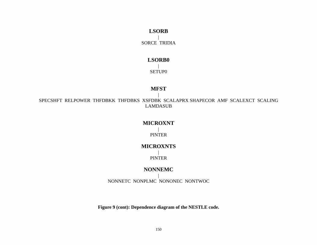
AMF SCALEXCT SCALING
.
150
LSORB|
SORCE TRIDIA
LSORB0|
SETUP0
MFST|
SPECSHFT RELPOWER THFDBKK THFDBKS XSFDBK SCALAPRX SHAPECORLAMDASUB
MICROXNT|
PINTER
MICROXNTS|
PINTER
NONNEMC|
NONNETC NONPLMC NONONEC NONTWOC
Figure 9 (cont): Dependence diagram of the NESTLE code

NTWOC
EARCH NONNEMC NONNEMHTRIDIA0 LSORB
.
151
NONNEMH|
NONNETH NONPLMH NONONEH NONTWOH NONONEC NO
NONONEC|
DIRECT4 DIRECT8B DIR4FULL DIR2FULL
NONONEH|
ONENODE4 ONENODE8
NONTWOC|
DIRECT4 DIRECT8B DIRECT8 DIRECT16
NONTWOH|
ONENODE4 ONENODE8 TWONODE8 TWONODE16
OUTIN|
GTIME LSORB CHEBY1 WEILANDT1 RELPOWER SXENON KSEARCH CNTROD PSTHFDBKS DEPLETE MFST RELPOWER SFST XSFDBK WSHIFT
Figure 9 (cont): Dependence diagram of the NESTLE code

ORB0
FDBKK MFST SFST XSFDBK
.
152
OUTINADJ|
GTIME LSORB CHEBY1 WEILANDT1 WSHIFT TRIDIA0 LS
OUTINTR|
GTIME LSORB CHEBYTR WEILANDTR NONNEMC NONNEMH RELPOWER THWSHIFT TRIDIA0
OUTPUTAD|
ANMERGE OUTPOINT
OUTPUTSS|
ANMERGE AVGEDIT OUTPOINT
OUTPUTTR|
ANMERGE AVGEDIT OUTPOINT
PERTURB|
LINEAR
Figure 9 (cont): Dependence diagram of the NESTLE code

RIDIA0 LSORB0 OUTIN PEAK
SHIFT TRIDIA0 LSORB0 OUTIN
.
153
PINPOWER|
PINFLX PINFLXMATA DIR12FULL
POINTER|
INPUTCK
SETUP0|
SORCE0 TRIDIA
SFST|
AMF SCALEXCT SCALING RELPOWER
SLOWTRAN|
PINTER XSFDBK OUTPCRT RELPOWER THFDBK TXENON CNTROD WSHIFT TOUTPCRT OUTPUTSS
STEADYN|
PINTER XSFDBK NORM NORMFSP SXENON RELPOWER THFDBKS CNTROD W
Figure 9 (cont): Dependence diagram of the NESTLE code

THFDBKK XSFDBK TRIDIA0OUTPUTTR
.
154
PEAK OUTPCRT
THFDBKK|
FLUIDCON
THFDBKS|
FLUIDCON
TRANSIT|
PERTURB NORM NORMFSP RELPOWER STARTER PRECR CNTROD TXENONOUTINTR RELPOWER DECAYHN UPDATE PEAK OUTPCRT
WEILANDT1|
RESID
WEILANDTR|
RESID
Figure 9 (cont): Dependence diagram of the NESTLE code

.
155
XSECBU|
PINTER
XSECBUS|
PINTER
Figure 9 (cont): Dependence diagram of the NESTLE code

ellet
rrently
ations.
linear
hecks
and
essage
SUBROUTINEADJOINTThis subroutine controls the calculation of the adjoint flux.
SUBROUTINEAMFThis subroutine determines (A-F)*flux for the fixed-source scale factor method.
SUBROUTINEANMERGEThis subroutine merges alphanumeric string arrays together to form single string.
SUBROUTINEAVGEDITThis subroutine edits out radial and axial core averaged properties.
SUBROUTINEAVGEDIT-PINThis subroutine edits out maximum value of axially-averaged pin power and maximum ppower.
SUBROUTINEBURNNODEThis subroutine solves the isotopic depletion equations.
SUBROUTINEBURNNODESThis subroutine solves the isotopic depletion equations on the six surfaces of a hexagon (cuworks for NSHAP= “HEXA” only).
SUBROUTINECALACVThis subroutine determines the interaction rates required to solve the isotopic depletion equ
SUBROUTNECHAINThis subroutine uses the integrating factor technique to analytically solve a coupleddepletion chain.
SUBROUTINECHEBY1This subroutine applies the semi-implicit Chebyshev polynomial acceleration method and cfor convergence for the steady state problem.
SUBROUTINECHEBYTRThis subroutine applies the semi-implicit CHEBYCHEV polynomial acceleration methodchecks for convergence for the transient problem.
SUBROUTINECHECKThis subroutines recognizes the different non-permissible runs and flags back an error malong with suggestion for the alternative run case.
Table 5: Listing of procedures and their functions.
156

uction
odel
odelf each
ector
d. All
ll
d. All
oyed..
SUBROUTINECNTRODThis subroutine determines the fraction of control group inserted.
SUBROUTINECONVERThis subroutine converts the input data units to NESTLE’s internal working units.
SUBROUTINECORNERFLXThis subroutines determines the corner point flux values needed for the pin power reconstr(currently works for NSHAP = “HEXA” only).
SUBROUTINEDECAYHNThis subroutine solves the decay heat precursor equations.
SUBROUTINEDEPLETEThis subroutine controls the depletion, determining number densities for the microscopic mand returning the macroscopic cross section expansion coefficients.
SUBROUTINEDEPLETESThis subroutine controls the depletion, determining number densities for the microscopic mand returning the macroscopic cross section expansion coefficients at the six surfaces ohexagonal assembly (currently works for NSHAP = “HEXA” only)
SUBROUTINEDIR12FULLThis subroutine solves a 12 x 12 matrix system needed for the pin power reconstruction. Varguments are employed. All unknowns are evaluated. Full matrix structure is assumed.
SUBROUTINEDIR2FULLThis subroutine analytically solves a 2 x 2 matrix system. Vector arguments are employeunknowns are evaluated. Full matrix structure is assumed in analytic solution.
SUBROUTINEDIR4FULLThis subroutine analytically solves a 4 x4matrix system. Vector arguments are employed. Aunknowns are evaluated. Full matrix structure is assumed in analytic solution.
SUBROUTINEDIRECT2X2This subroutine analytically solves a 2 x 2 matrix system. No vector arguments are employeunknowns are evaluated. Full matrix structure is assumed in analytic solution.
SUBROUTINEDIRECT16This subroutine analytically solves a 16 x 16 matrix system. Vector arguments are emplOnly half of unknowns are evaluated. Matrix sparsity is taken advantage in analytic solution
Table 5 (cont): Listing of procedures and their functions.
157

ll
d. All
d. All
ed for
rovides
ternal
gather
SUBROUTINEDIRECT4This subroutine analytically solves a 4 x4matrix system. Vector arguments are employed. Aunknowns are evaluated. Matrix sparsity is taken advantage in analytic solution.
SUBROUTINEDIRECT8This subroutine analytically solves a 8 x 8 matrix system. Vector arguments are employeunknowns are evaluated. Matrix sparsity is taken advantage in analytic solution.
SUBROUTINEDIRECT8BThis subroutine analytically solves a 8 x 8 matrix system. Vector arguments are employeunknowns are evaluated. Matrix sparsity is taken advantage in analytic solution.
SUBROUTINEECHOINPThis subroutine echoes out the radial input figures.
SUBROUTINEFILE_CNTThis subroutine reads the general control input parameters.
SUBROUTINEFILE_GEOThis subroutine reads the geometrical parameters.
SUBROUTINEFILE_KINThis subroutine reads the kinetic parameters required for the transient runs.
SUBROUTINEFILE_PPRThis subroutine reads the corner point discontinuity factors and pin-wise form factors needthe pin power reconstruction (currently works for NSHAP = “HEXA” only).
SUBROUTINEFILE_PRFThis subroutine reads the parameters used to control the solution methods employed and pthe convergence criteria.
SUBROUTINEFILE_XSCThis subroutine reads the cross sections and T-H input parameters.
SUBROUTINEFLUIDCONThis subroutine calculates coolant temperature, density, and void fraction based upon inenergy.
SUBROUTINEGASCATCThis subroutine is used for the cart geometry only. It calculates the needed parameters tothe nodes with the same color together (i.e. blacks with blacks...etc). for Cartesian geometry, two
Table 5 (cont): Listing of procedures and their functions.
158

.
gatheree.
ndary
AIX
ulateve the
start
rol
ntrol,
rything
inlet
different colors are used. this will be utilized in the solution of the finite difference equations
SUBROUTINE GASCATHThis subroutine is used for the hex geometry only. It calculates the needed parameters tothe nodes with same color together (i.e. blacks with blacks...etc). For Hexagonal geometry, thrdifferent colors are used. this will be utilized in the solution of the finite difference equations
SUBROUTINEGEOMETRYThis subroutine sets up the geometry including B.C. mesh expansion and bundle bouidentification for output control.
FUNCTION GTIMEThis subroutine returns back the elapsed time (in seconds) applicable to ULTRIX oroperating system.
SUBROUTINEHYPINTThis subroutine contains three functions: COSH0, SINH1, COSH2. The three functions calcthe zeroth, first, and second moment integration of the hyperbolic functions needed to solconformal mapping based hexagonal nodal equations. (For NSHAP = “HEXA” only).
SUBROUTINEINITALThis subroutine initializes the flux, fission source, and T-H conditions guesses, or for reoption on reads in the restart file.
SUBROUTINEINIVALThis subroutine edits out the initial input data.i.e. cross section data, geometry data, and contoptions, if users choose long edits for the inputs (AL3 = “Y”).
SUBROUTINEINPDATAThis subroutine controls the overall input reading.
SUBROUTINEINPEDITThis subroutine edits out input associated with the transient case, method of solution cocontrol options, I/O file names, and if elected cross sections and T-H parameters.
SUBROUTINEINPUTCKThis subroutine checks whether alphanumeric input was correctly entered and converts eveto upper case letters.
SUBROUTINEKSEARCHThis subroutine performs criticality search on four different parameters: soluble poison,coolant temperature, power level, and control bank insertion.
Table 5 (cont): Listing of procedures and their functions.
159

laroutine
for the
letable
letable
every
SUBROUTINELAMDASUBThis subroutine determines the scale factor for the fixed-source scale factor method.
SUBROUTINELINEARThis subroutine completes the linear interpolation or extrapolation.
SUBROUTINELSORBThis subroutine calls the following two subroutines:SORCE - which calculates the RHS of the finite difference equations for a specific color.TRIDIA - which solves for the flux by solving a tridiagonal system of equations for a particucolor. The flux is also accelerated using the omegas which were precalculated in the subrLSORB0.
SUBROUTINELSORB0This subroutine calculates the number of inner per outer and the acceleration parameterscolor line SOR equations.
PROGRAMMAINThis is the main routine for NESTLE.
SUBROUTINEMFSTThis subroutine controls the multi fixed source scale factor method.
SUBROUTINEMICROXNTThis subroutine determines the microscopic cross section expansion coefficients for the depisotopes.
SUBROUTINEMICROXNTSThis subroutine determines the microscopic cross section expansion coefficients for the depisotopes on the six surface of the hexagonal assembly (NSHAP = “HEXA” only).
FUNCTION NEWPAGEStarts a new page of output.
SUBROUTINENONNEMCThis subroutine solves the NEM equations.********* For Cartesian Geometry **************The nodal method used here is nonlinear NEM, We solve a one or two node problem forinterface in the core to update the coupling coefficients.
SUBROUTINENONNEMHThis subroutine solves the NEM equations.
Table 5 (cont): Listing of procedures and their functions.
160

ometry.pling
urrent
urrent
nsion
nsion
.
********* For Hexagonal Geometry **************The nodal method used here is a conformal mapping based nodal method for hexagonal geWe solve a one or two node problem for every interface in the core to update the coucoefficients.
SUBROUTINENONNETCThis subroutine determines the currents for NEM.********* For Cartesian Geometry **************
SUBROUTINENONNETHThis subroutine determines the currents for NEM.********* For Hexagonal Geometry **************
SUBROUTINENONONECThis subroutine solves a one-node problem. It is used only for edge nodes without zero cboundary condition when updating the net currents by NONNEM.********* For Cartesian Geometry **************
SUBROUTINENONONEHThis subroutine solves a one-node problem. It is used only for edge nodes without zero cboundary condition when updating the net currents by NONNEM.********* For Hexagonal Geometry **************
SUBROUTINENONPLMCThis subroutine calculates the leakages for every node in every direction and the expacoefficients for the quadratic leakage approximation.********* For Cartesian Geometry **************
SUBROUTINENONPLMHThis subroutine calculates the leakages for every node in every direction and the expacoefficients for the quadratic leakage approximation.********* For Hexagonal Geometry **************
SUBROUTINENONTWOCThis subroutine solves the two node problem and returns the NEM current JNEM.********* For Cartesian Geometry **************
SUBROUTINENONTWOHThis subroutine solves the two node problem and returns the NEM current JNEM.********* For Hexagonal Geometry **************
SUBROUTINENORMThis subroutine normalizes the flux and fission source to a core relative average power = 1
Table 5 (cont): Listing of procedures and their functions.
161

d. All
d. All
tate
int
ient
st.
SUBROUTINENORMFSPThis subroutine normalizes the flux and fission source to an input specified scaling.
SUBROUTINEONENODE4This subroutine analytically solves a 4 x 4 matrix system. Vector arguments are employeunknowns are evaluated. Matrix sparsity is taken advantage in analytic solution.
SUBROUTINEONENODE8This subroutine analytically solves a 8 x 8 matrix system. Vector arguments are employeunknowns are evaluated. Matrix sparsity is taken advantage in analytic solution.
SUBROUTINEOUTCYCThis subroutine writes the node-wise isotopic number densities.
SUBROUTINEOUTINThis subroutine performs outer-inner iterations utilizing FDM or NEM option for the steady ssolution.
SUBROUTINEOUTINADJThis subroutine performs outer-inner iterations utilizing FDM or NEM option for the adjosolution.
SUBROUTINEOUTINTRThis subroutine performs outer-inner iterations utilizing FDM or NEM option for the transsolution.
SUBROUTINEOUTPCRTThis subroutine outputs values to the screen (i.e.CRT).
SUBROUTINEOUTPOINTThis subroutine outputs point-wise values of parameter passed through calling argument li
SUBROUTINEOUTPUTADThis subroutine outputs the adjoint problem’s solution.
SUBROUTINEOUTPUTSSThis subroutine outputs the steady state problem’s solution.
SUBROUTINEOUTPUTTRThis subroutine outputs the transient problem’s solution.
Table 5 (cont): Listing of procedures and their functions.
162

.
group>2
ower
e two-
gian
, inlet
les the
lerkin
SUBROUTINEPEAKThis subroutine determines the total peaking factor and location.
SUBROUTINEPERTURBThis subroutine interpolates the time dependent input parameters for the transient problem
SUBROUTINEPINCOLLAPThis subroutine collapses kappa-sigma-fission cross sections and fluxes for NG>2 into two-cross sections and fluxes for the pin power reconstruction (NSHAP = “HEXA” only). NGintroduces complexities in determining pin-wise fluxes.
SUBROUTINEPINLOCThis subroutine determines the fuel pin locations within the hexagonal assembly for the pin preconstruction (NSHAP = “HEXA” only).
SUBROUTINEPINPOWERThis subroutine performs a pin power reconstruction in hexagonal geometry based upon thgroup cross sections and fluxes (NSHAP = “HEXA” only).
SUBROUTINEPINTERThis subroutine completes quadratic interpolation (or extrapolation) using Lagranpolynomial.
SUBROUTINEPOINTERThis subroutine determines the A array pointers (i.e.starting locations of arrays).
SUBROUTINEPRECRThis subroutine solves the delayed neutron precursor equations.
FUNCTION PROPPOLYThis subroutine calculates specified property as function of a stated dependence.
SUBROUTINEPSEARCHThis subroutine performs power level search on three different parameters: soluble poisoncoolant temperature, and control bank insertion.
SUBROUTINERELPOWERThis subroutine determines the total core power level accounting for decay heat and scapower density to a relative core power level = 1.
SUBROUTINERESIDDetermines the relative residual of the diffusion equation and the eigenvalue using Ga
Table 5 (cont): Listing of procedures and their functions.
163

ed by
cale
ource
ining
steady
factor
IDIA.e the, and
IDIA.Theed inouter
weighting of the diffusion operators.
SUBROUTINERSTRINGThis subroutine loads a numeric value into an alphanumeric variable.
SUBROUTINESCALAPRXThis subroutine calculates the ratio of the effective external source to the fission source usthe fixed-source scale factor method.
SUBROUTINESCALEXCTThis subroutine determines the ratio of the effective external source to (A-F)*FLUX to get sfactor update.
SUBROUTINESCALINGThis subroutine scales the flux and fission source using the scale factor from the fixed-sscale factor method.
SUBROUTINESETUP0This subroutine solves the homogeneous problem using color line G-S in support of determoptimum relaxation parameters and number of iterations per outer iteration.
SUBROUTINESFSTThis subroutine performs the single fixed-source scaling technique procedure for the FSPstate case.
SUBROUTINESHAPECORThis subroutine adjusts the flux for coolant spectral effects within the fixed-source scalemethod.
SUBROUTINESLOWTRANThis subroutine provides overall control of the transient fission product problem.
SUBROUTINESORCEThis subroutine calculates the RHS for the tridiagonal system to be solved by subroutine TRThe tridiagonal system results from using the color line SOR method which is used to solvfinite difference form of the diffusion equations. The RHS here includes fission, scatteringdiffusion terms.
SUBROUTINESORCE0This subroutine calculates the RHS for the tridiagonal system to be solved by subroutine TRThe equation to be solved is A*PHI=0 where A is the coefficient matrix and PHI is the flux.RHS here does not include any fission or scattering. It only includes diffusion terms. It is usobtaining the color line SOR extrapolation parameters and number of inner iterations per
Table 5 (cont): Listing of procedures and their functions.
164

ion in
ts.
for the
for the
r line
ys for
ctorge in
ctorge in
iteration.
SUBROUTINESPECSHFTThis subroutine determines the B**2 values used in making the coolant spectral shift correctthe fixed-source scale factor method.
SUBROUTINESTARTERThis subroutine sets initial values to initiate the transient from.
SUBROUTINESTEADYNThis subroutine provides overall control of the steady state solution.
SUBROUTINESXENONThis subroutine solves for the steady state number densities of the transient fission produc
SUBROUTINETHFDBKKThis subroutine calculates coolant internal energy, coolant density, and fuel temperaturestransient problem.
SUBROUTINETHFDBKSThis subroutine calculates coolant internal energy, coolant density, and fuel temperaturessteady state problem.
SUBROUTINETRANSITThis subroutine provides overall control of the transient problem.
SUBROUTINETRIDIAThis subroutine solves a tridiagonal system of equation which results from using the coloSOR method. It solves for the flux of a particular color each time it is called.
SUBROUTINETRIDIA0This subroutine factors the tridiagonal matrices associated with color line and assigns to arraeach color.
SUBROUTINETWONODE8This subroutine analytically solves a 8 x 8 matrix system used in NONTWOH routine. Vearguments are employed. All unknowns are evaluated. Matrix sparsity is taken advantaanalytic solution.
SUBROUTINETWONODE16This subroutine analytically solves a 16 x 16 matrix system used in NONTWOH routine. Vearguments are employed. All unknowns are evaluated. Matrix sparsity is taken advantaanalytic solution.
Table 5 (cont): Listing of procedures and their functions.
165

e step
for
for
roup
eption.
sion
ity, fuel
ity, fuelnsion
ity, fuel
SUBROUTINETXENONThis subroutine solves for the transient number densities of the transient fission products.
SUBROUTINEUPDATEThis subroutine saves time-step values of various parameters for usage in the next timsolution.
SUBROUTINEWEILANDT1This subroutine is applicable to Wielandt shift with stationary acceleration and checksconvergence for the steady state problem.
SUBROUTINEWEILANDTRThis subroutine is applicable to Wielandt shift with stationary acceleration and checksconvergence for the transient problem.
SUBROUTINEWSHIFTThis subroutine determines Wielandt shift utilizing the Sutton method to retain energy gdecoupling at inner iterative level.
SUBROUTINEXSECBUThis subroutine determines the nuclear properties (e.g.cross section expansion coefficients) at thnode color and burnup except for the depletable isotopes modeled using the microscopic o
SUBROUTINEXSECBUCThis subroutine determines the corner point discontinuity factor and form factor expancoefficients (NSHAP = “HEXA” only).
SUBROUTINEXSECBUSThis subroutine determines the surfaces’ nuclear properties,e.g. cross section expansioncoefficients (NSHAP = “HEXA” only).
FUNCTION XSECPOLYThis subroutine calculates cross sections accounting for coolant temperature, coolant denstemperature and soluble poison feedback corrections.
FUNCTION XSECPOLY2This subroutine calculates cross sections accounting for coolant temperature, coolant denstemperature and soluble poison feedback corrections. Difference with XSECPOLY is dimeof calling arguments arrays.
FUNCTION XSECPOLYSThis subroutine calculates cross sections accounting for coolant temperature, coolant dens
Table 5 (cont): Listing of procedures and their functions.
166

agonal
djoint
utronic
utronic
rnup
temperature and soluble poison feedback corrections on the six surfaces of the hexassembly (NSHAP = “HEXA” only).
SUBROUTINEXSFDADJThis subroutine determines the matrix transpose of the coefficient matrix required for the aflux solution.
SUBROUTINEXSFDBKThis subroutine determines the macroscopic and microscopic cross sections and other nenode values and uses them in determining the coefficient matrix.
SUBROUTINEXSFDBKSThis subroutine determines the macroscopic and microscopic cross sections and other nevalues on the six surfaces of a hexagonal assembly (NSHAP = “HEXA” only).
SUBROUTINEXSMODThis subroutine calculates the flux-volume weighted cross sections for the within-node bugradient treatment in the hexagonal nodal method (NSHAP = “HEXA” only).
Table 5 (cont): Listing of procedures and their functions.
167

adf.fcb cntl2.fcb hexdim.fcb perttr.fcb thermo.fcbadj.fcb confmap.fcb hgeo.fcb pertv.fcb thmargin.fcbarray.fcb conv.fcb multit.fcb pinpow.fcb tim.fcbbasic.fcb convfact.fcb nemcnt.fcb power.fcb time.fcbbcs.fcb crhs.fcb nemtime.fcb restinp.fcb time1.fcbbcshex.fcb crit.fcb nline.fcb restotp.fcb timetr.fcbbpitch.fcb crod.fcb nonfue.fcb rodkin.fcb varlen.fcbbuckl.fcb dataf.fcb nterm.fcb soln2.fcb varlens.fcbbundle.fcb depletepc.fcb numsurf.fcb spectral.fcb veloc.fcbburn.fcb extsor.fcb only.fcb srf.fcb xeopt.fcbbypass.fcb flamdold.fcb opti.fcb start.fcb xsec1.fcbche.fcb fpxs.fcb outlong.fcb th_cof.fcb xsec2.fcbcheby.fcb gasch.fcb param.fcb thcoef.fcb xspolycom.fcbcntl.fcb geom.fcb pardrwm.fcb thermk.fcb
Table 6: Listing of fcb files containing named COMMON blocks
168

View publication statsView publication stats
NESTLE NESTLE NESTLE NESTLE NESTLE NESTLE NESTLE NESTLE NESTLE NESTLE NESTLE NESTLE NESTLE NESTLE NESTLE NESTLE NESTLE NESTLE NESTLE NESTLE NESTLE NESTLE NESTLE NESTLE NESTLE VERSION 1.0 NESTLE NESTLE ELECTRIC POWER RESEARCH CENTER NESTLE NESTLE NORTH CAROLINA STATE UNIVERSITY NESTLE NESTLE COPYRIGHT 1994 - BY NCSU NESTLE NESTLE NESTLE NESTLE NESTLE DICTIONARY PROGRAM NESTLE NESTLE NESTLE NESTLE NESTLE NESTLE NESTLE NESTLE NESTLE NESTLE NESTLE NESTLE NESTLE NESTLE NESTLE NESTLE NESTLE NESTLE NESTLE NESTLE NESTLE NESTLE NESTLE NESTLE NESTLE
WHICH OPTION DO YOU WISH TO ENABLE (E=EXIT, F=FIND, D=DELETE, A=ADD)? F
WHAT IS THE VARIABLE NAME THAT YOU WISH THE DEFINITION FOUND FOR?SW
DEFINITION: MESH DEPENDENT FLUX [SOLUTION TO THE PROBLEM] / EIGENVECTOR FOR THE EIGENVALUE PROBLEM
WHICH OPTION DO YOU WISH TO ENABLE (E=EXIT, F=FIND, D=DELETE, A=ADD)? A
WHAT IS THE VARIABLE NAME YOU WISH TO ADD? TEST1
INPUT DEFINITION FOR THE VARIABLE:JUST A TEST VARIABLE FOR THE DICTIONARY PROGRAM
WHICH OPTION DO YOU WISH TO ENABLE(E=EXIT, F=FIND, D=DELETE, A=ADD)?F
WHAT IS THE VARIABLE NAME THAT YOU WISH THEDEFINITION FOUND FOR? TEST1
DEFINITION:JUST A TEST VARIABLE FOR THE DICTIONARY PROGRAM
WHICH OPTION DO YOU WISH TO ENABLE (E=EXIT, F=FIND, D=DELETE, A=ADD)? D
WHAT IS THE VARIABLE NAME THAT YOU WISH THE DEFINITION DELETED FOR?TEST1
ARE YOU CERTAIN THAT YOU WANT THE VARIABLE DEFINITION DELETED (Y,N)?Y
VARIABLE DEFINITION DELETED.
WHICH OPTION DO YOU WISH TO ENABLE (E=EXIT, F=FIND, D=DELETE, A=ADD)?E
IF VARIABLE NAMES AND DEFINITIONS HAVE BEEN ADDED OR DELETED, DO YOU WANT TO SAVE CHANGES IN DATA BASE (Y,N)?Y
Table 7: Sample interactive session with NESTLE.DICT
169